the Creative Commons Attribution 4.0 License.
the Creative Commons Attribution 4.0 License.
 | 18 Feb 2021
First investigation of perennial ice in Winter Wonderland Cave, Uinta Mountains, Utah, USA
Winter Wonderland Cave is a solution cave at an elevation of 3140 m above sea level in Carboniferous-age Madison Limestone on the southern slope of the Uinta Mountains (Utah, USA). Temperature data loggers reveal that the mean annual air temperature (MAAT) in the main part of the cave is −0.8 ∘C, whereas the entrance chamber has a MAAT of −2.3 ∘C. In contrast, the MAAT outside the cave entrance was +2.8 ∘C between August 2016 and August 2018. Temperatures in excess of 0 ∘C were not recorded inside the cave during that 2-year interval. About half of the accessible cave, which has a mapped length of 245 m, is floored by perennial ice. Field and laboratory investigations were conducted to determine the age and origin of this ice and its possible paleoclimate significance. Ground-penetrating-radar (GPR) surveys with a 400 MHz antenna reveal that the ice has a maximum thickness of ∼ 3 m. Samples of rodent droppings obtained from an intermediate depth within the ice yielded radiocarbon ages from 40±30 to 285±12 years. These results correspond with median calibrated ages from CE 1560 to 1830, suggesting that at least some of the ice accumulated during the Little Ice Age. Samples collected from a ∼ 2 m high exposure of layered ice were analyzed for stable isotopes and glaciochemistry. Most values of δ18O and δD plot subparallel to the global meteoric waterline with a slope of 7.5 and an intercept of 0.03 ‰. Values from some individual layers depart from the local waterline, suggesting that they formed during closed-system freezing. In general, values of both δ18O and δD are lowest in the deepest ice and highest at the top. This trend is interpreted as a shift in the relative abundance of winter and summer precipitation over time. Calcium has the highest average abundance of cations detectable in the ice (mean of 6050 ppb), followed by Al (2270 ppb), Mg (830 ppb), and K (690 ppb). Most elements are more abundant in the younger ice, possibly reflecting reduced rates of infiltration that prolonged water–rock contact in the epikarst. Abundances of Al and Ni likely reflect eolian dust incorporated in the ice. Liquid water appeared in the cave in August 2018 and August 2019, apparently for the first time in many years. This could be a sign of a recent change in the cave environment.
- Article
(10180 KB) - Full-text XML
- BibTeX
- EndNote


Caves containing perennial ice, hereafter known as “ice caves”, have been reported from around the world (Perşoiu and Lauritzen, 2017). Local permafrost conditions are maintained in these caves due to a combination of cold-air trapping and dynamic ventilation (Luetscher and Jeannin, 2004a). Ice in these caves is a product of firnification of snow that falls or slides into the entrance, congelation of water entering into the cave, or both. Previous studies have demonstrated the paleoclimate potential of the perennial ice in caves (Holmlund et al., 2005; Perşoiu et al., 2017), which can be investigated with methods analogous to those applied to glacier ice cores (Yonge and MacDonald, 1999, 2014). Significantly, because ice caves are present at lower latitudes and altitudes than many mountain glaciers, they provide an opportunity to expand cryosphere-based paleoclimate records to areas where surficial ice is absent (Perşoiu and Onac, 2012). An important motivation for increased study of ice caves is the observation that many perennial ice bodies in these caves are currently melting (Fuhrmann, 2007; Kern and Thomas, 2014; Pflitsch et al., 2016). This worrisome trend raises the alarm that the paleoclimate records preserved in these subterranean ice masses will be lost forever (Kern and Perşoiu, 2013; Veni et al., 2014).
Despite the exciting potential of ice caves as paleoclimate archives, these features remain an understudied component of the cryosphere. Although an overview of ice caves in a variety of settings was presented more than 100 years ago (Balch, 1900), most modern investigations of cave ice have been conducted in a few focused areas, particularly the Alps (e.g., Luetscher et al., 2005; May et al., 2011; Morard et al., 2010) and the mountains of Romania (e.g., Perşoiu et al., 2011; Perşoiu and Pazdur, 2011). There, techniques for dating cave ice (e.g., Kern et al., 2009; Luetscher et al., 2007; Spötl et al., 2014), interpreting stable-isotope records in cave ice (e.g., Kern et al., 2011b; Perşoiu et al., 2011), and studying the glaciochemistry (e.g., Carey et al., 2019; Kern et al., 2011a) of cave ice have been developed over the past several decades. Technologies such as environmental data loggers have simultaneously enabled investigation of micrometeorology in ice caves (e.g., Luetscher and Jeannin, 2004b; Obleitner and Spötl, 2011), and geophysical techniques such as ground-penetrating radar (GPR) have been employed to image ice stratigraphy (e.g., Behm and Hausmann, 2007; Colucci et al., 2016; Gómez Lende et al., 2016; Hausmann and Behm, 2011). In general, however, these techniques have been employed only on a limited basis elsewhere in the world. In North America, the ablation of subterranean ice masses has been monitored in New Mexico (Dickfoss et al., 1997) as well as in lava tubes on the Big Island of Hawaii (Pflitsch et al., 2016) and in California (Fuhrmann, 2007; Kern and Thomas, 2014). Seminal work on stable isotopes in cave ice was conducted in the Canadian Rocky Mountains (Lauriol and Clark, 1993; Yonge and MacDonald, 1999, 2014), and micrometeorology studies have been published on sites with (possibly) perennial ice in the northern Appalachian Mountains (Edenborn et al., 2012; Holmgren et al., 2017).
The most extensive investigation of a North American ice cave focused on Strickler Cavern, a site in the Lost River Range of Idaho (Munroe et al., 2018). That work documented coexistence of firn ice and congelation ice with radiocarbon age control extending back ∼ 2000 years. Stable isotopes in this ice were interpreted to record cooling temperatures leading into the Little Ice Age, and analysis of major and trace elements supported identification of a local component and an exotic component of the overall dissolved load in the ice.
The project presented here applied the successful multidisciplinary approach from Strickler Cavern (Munroe et al., 2018) to another cave containing ice of a different genesis. In addition to radiocarbon dating and glaciochemical and isotopic analysis, a 2-year deployment of temperature data loggers was incorporated to constrain cave meteorology, and GPR was employed to determine the thickness of the perennial ice body. The primary objectives of the project were to
-
determine the origin, extent, and age of the ice in this cave;
-
develop and interpret a stable-isotope record for this ice;
-
analyze and interpret the glaciochemistry of the ice.
2.1 Field site
Fieldwork was conducted within Winter Wonderland Cave in the Uinta Mountains of northeastern Utah, USA. Winter Wonderland Cave (hereafter “WWC”) was discovered in 2012 and has an entrance at an elevation of 3140 m on a north-facing cliff. The cave is developed in the Carboniferous-age Madison Limestone, a regionally extensive rock unit that in this area consists of fine- to coarse-grained dolomite and limestone, with locally abundant nodules of chert (Bryant, 1992). The general location is presented in Fig. 1, but to preserve this fragile cave environment and the ice formations within it, the exact coordinates of the cave entrance are withheld. The cave has a vertical extent of 33 m and a mapped length of 245 m (Fig. 1c). The narrow entrance slopes down steeply ∼ 10 m to a roughly circular room (∼ 10 m diameter) with a high ceiling and flat floor of ice. From this “Icicle Room” a narrow crack leads off to intersect with the “Frozen Freeway”, a larger passage that forms the main part of the cave. This steep-sided canyon, with walls up to 8 m high, developed along a vertical fracture bearing 160∘ (or 340∘). Similar steeply dipping fractures, at spacings ranging from ∼ 20 to >200 cm, are responsible for the porosity and permeability of the limestone host rock. The part of the Frozen Freeway closer to the Icicle Room is a descending slope of breakdown derived from the cave ceiling. Beyond this section, most of the floor of the Frozen Freeway is ice (Fig. 1c). The Frozen Freeway terminates in a wider section with an ice floor called the “Skating Rink”. Beyond the Skating Rink, the cave splits into two passages, both of which are choked with rock debris. Strong air currents passing through these rock piles suggest the presence of considerable additional passage beyond the chokes. This air current has sublimated the ice at the edge of the Skating Rink, producing an exposure ∼ 2 m tall (Fig. 1c).
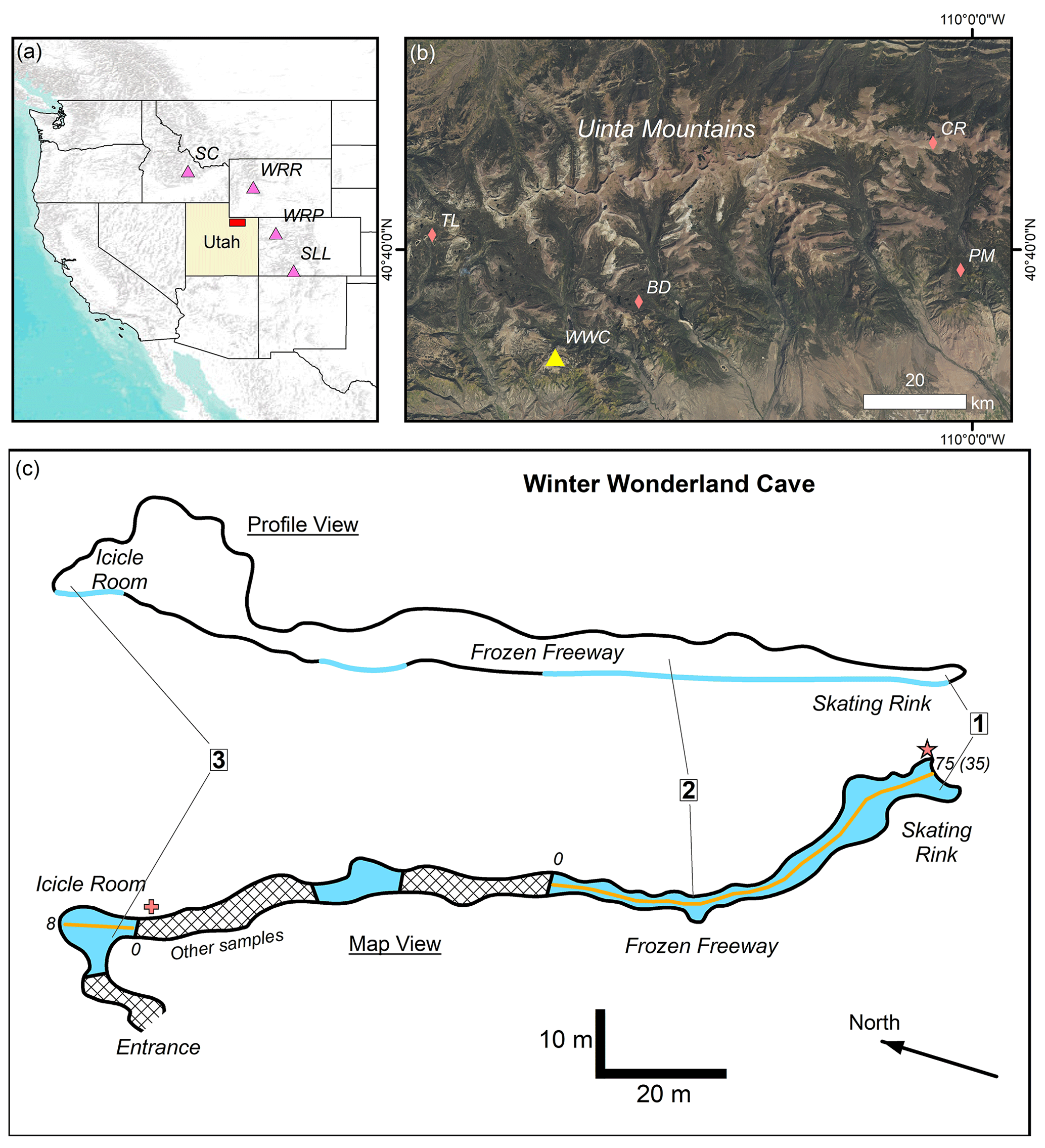
Figure 1Location map of the study area. (a) Western North America with US state outlines. The state of Utah is highlighted. The red box denotes the location of the enlargement in panel (b). Other sites noted in the text are identified: Strickler Cavern (SC; Munroe et al., 2018), Wind River Range (WRR; Naftz et al., 1996), White River Plateau (WRP; Anderson, 2012), San Luis Lake (SLL; Yuan et al., 2013). (b) Enlargement of the Uinta Mountain region in USA National Agricultural Imagery Program (NAIP) natural color imagery. The yellow triangle marks the location of Winter Wonderland Cave (WWC). Other sites noted in the text are identified: Trial Lake (TL) snowpack-monitoring site and snow sampling site, Brown Duck (BD) snowpack-monitoring site, Pole Mountain (PM) snow sampling site, Chepeta remote automated weather station (RAWS; CR). (c) Profile and map views of Winter Wonderland Cave simplified from mapping by David Herron, USDA Forest Service. The cross-hatching pattern denotes breakdown, and the blue color denotes perennial ice. The locations of the cave entrance, the Icicle Room, the Frozen Freeway, and the Skating Rink are noted. The orange lines mark the ground-penetrating radar transects. The numbers 0 and 75 mark the start and end of the transect in the Frozen Freeway. Only the last 35 m of this transect are interpreted in the text. The numbers 0 and 8 mark the start and end of the transect in the Icicle Room. The red star at the end of the Skating Rink is the exposure described in the text. The red cross marks the exposure at the edge of the Icicle Room. “Other samples” highlights the region where additional local ice samples were collected from between blocks of breakdown. The boxed numerals 1–3 identify the locations of the temperature data loggers.
Fieldwork focused on documenting the temperature conditions within WWC, determining the thickness of the perennial ice, gathering organic remains for radiocarbon dating, and collecting ice samples for glaciochemical and isotopic analysis. Visits to WWC for this project were made on 11 August 2016, 29 August 2018, and 19 August 2019.
2.2 Cave temperature monitoring
Three temperature data loggers (Onset Temp Pro v2) were deployed within the cave from August 2016 through August 2018 (Fig. 1c). Each logger was suspended from the ceiling to measure temperature of the free air ∼ 30 cm away from the rock walls and ice surface. The loggers were set to record the temperature every hour. An additional logger was deployed within a solar-radiation shield outside the cave entrance to record ambient air temperatures. The temperature data loggers were collected in late August 2018. Data were downloaded into the proprietary Onset software Hoboware, filtered to calculate daily mean values, and exported to a spreadsheet for further analysis and plotting.
2.3 Ground-penetrating radar
To constrain the thickness of the ice, GPR surveys were conducted along the Frozen Freeway in 2019 following standard protocols (e.g. Hausmann and Behm, 2011). A shielded 400 MHz antenna and a GSSI SIR-3000 controller were used to collect the radar data. Before the survey, a transect was established with measured points every 5 m. A mark was recorded in the GPR data each time the antenna passed one of these points, which allowed the GPR results to be converted to a physical horizontal scale. A shorter survey was also conducted in the Icicle Room. In both locations, surveys were conducted multiple times, in both directions. Gain settings were determined using an auto-gain procedure at the start of each transect to optimize the balance between detecting stratigraphy in the ice and simultaneously imaging the underlying ice–rock interface.
Data collected with the GPR were processed with Radan 7.0. Processing involved standard steps (e.g., Colucci et al., 2016; Hausmann and Behm, 2011), including a time-zero correction to eliminate the impulse passing directly from the antenna to receiver (the direct wave); a full-pass background removal to remove the surface wave; a finite impulse response (FIR) stacking filter to remove airwave reflections from the cave walls; an additional FIR filter to clip the bandwidth between 300 and 700 MHz; an adaptive gain procedure to amplify faint, deeper reflectors; distance normalization to produce a scaled profile; and migration to remove hyperbolic reflectors produced by objects within the ice. A dielectric permittivity of 3.15, typical of pure ice (Thomson et al., 2012) and corresponding to an average velocity of ∼ 0.16 m/ns, was used to convert two-way radar travel times to estimated depths below the surface of the ice. Because the focus was on determining the thickness of the ice, no attempt was made to account for the different permittivity of the underlying bedrock.
2.4 Geochronology
To constrain the age of the ice, rodent droppings within the ice were retrieved by angling an ice screw so that it intersected with the dropping and raised it to the surface. This technique was limited to droppings visible within the upper 15 cm of the ice, corresponding to the length of the ice screw. However, because the surface of the ice was locally sublimated into a series of valleys and troughs with relief of ∼ 30 cm, drilling in the base of the troughs permitted the retrieval of droppings from deeper levels beneath the original ice surface. Samples were collected along the length of the Frozen Freeway (Fig. 2); depths of these samples were estimated relative to the height of the nearest ridge on the sublimated ice surface (Table 1). An additional sample was collected from a depth of ∼ 75 cm below the ice surface in the Icicle Room, taking advantage of a vertical exposure of ice eroded by air currents entering from the Frozen Freeway.
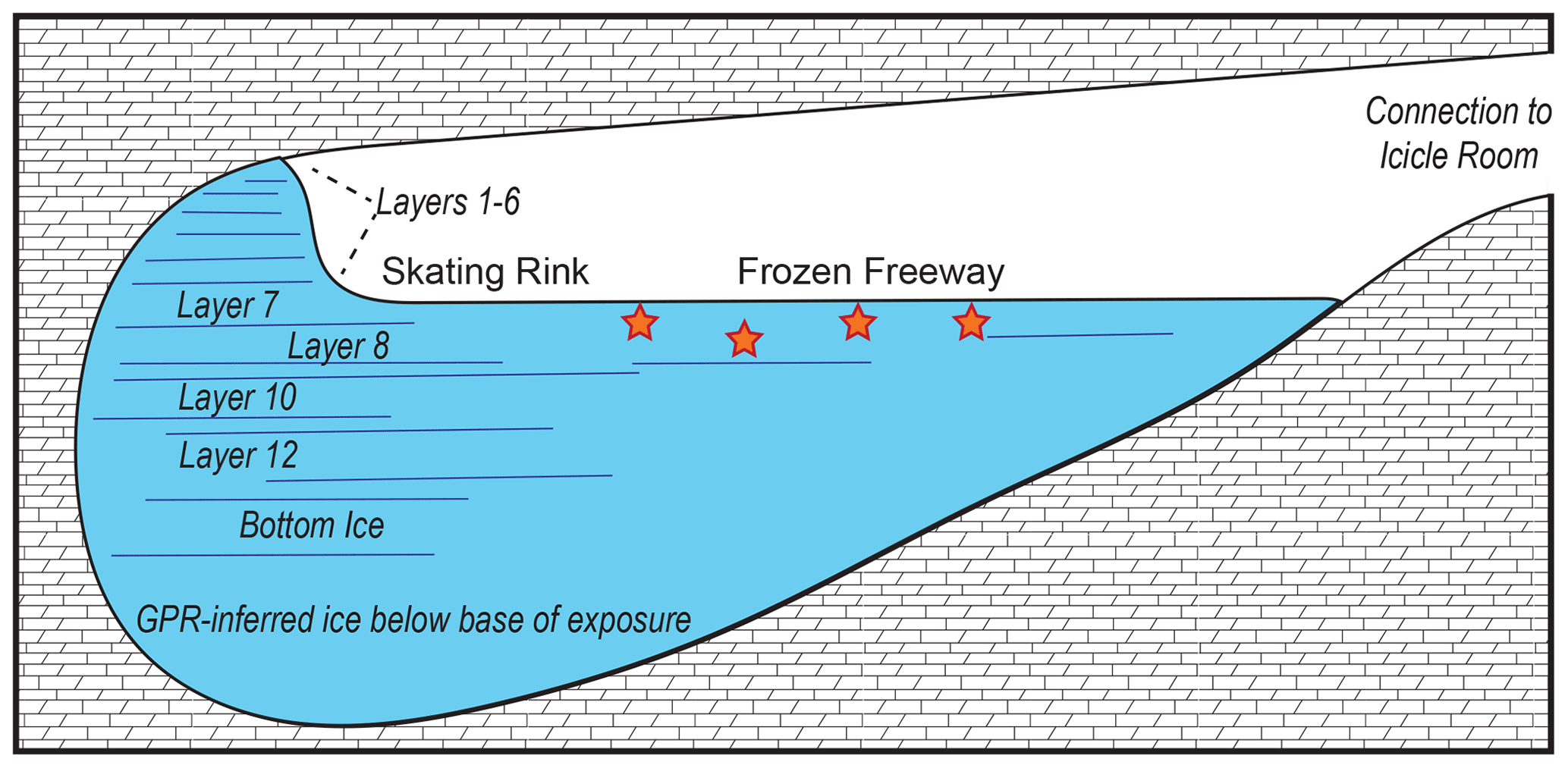
Figure 2Schematic illustrating the relationship between the Frozen Freeway, where most 14C samples were collected from shallow depths within the ice, and the taller exposure at the Skating Rink, where most samples for stable isotopes and glaciochemistry were collected. This exposure reached to the cave ceiling, and the part projecting above the Frozen Freeway contained six visibly distinct layers. Intermediate parts of this exposure were also visibly layered, with Layers 7 and 8 corresponding stratigraphically to the near-surface layers of the Frozen Freeway, where the 14C samples were collected. The bottom ice in this exposure did not appear to be layered, although it was difficult to view this ice directly. The total height of the Skating Rink exposure is 2 m.
Table 1Radiocarbon dating results from Winter Wonderland Cave.
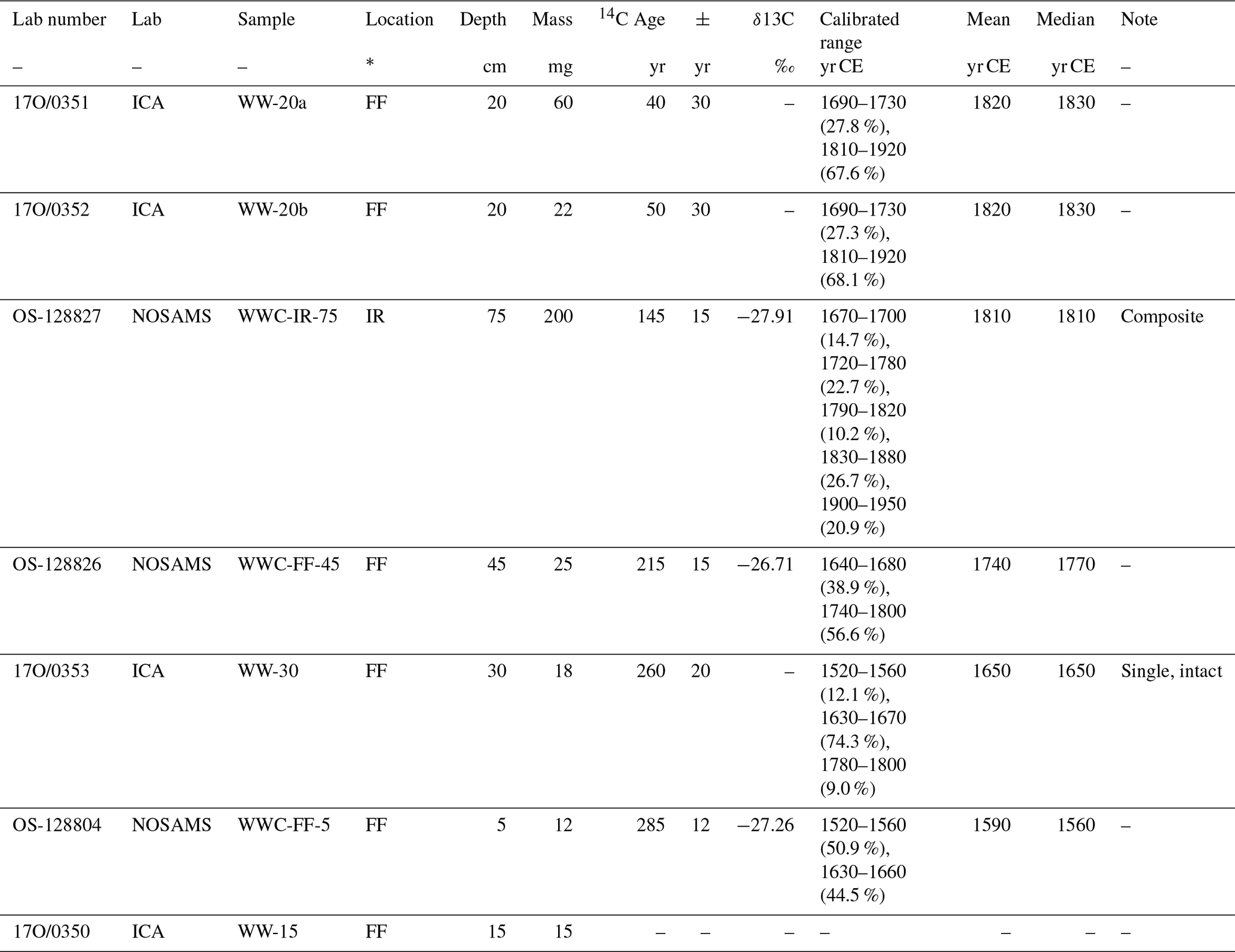
* FF: Frozen Freeway; IR: Icicle Room.
Samples of rodent droppings were selected for AMS 14C dating at NOSAMS (National Ocean Sciences Accelerator Mass Spectrometry facility) and ICA (International Chemical Analysis Inc.). Each was dried, weighed, and photographed before submission. Resulting radiocarbon ages were calibrated against the IntCal 20 calibration curve data (Reimer et al., 2020) in Oxcal 4.4. All of the samples yielded multiple possible calibration ranges.
2.5 Isotopic and glaciochemical analyses
Ice samples were collected from existing exposures using an approach similar to that employed in previous studies (e.g., Carey et al., 2019). Using a hand-operated ice screw, a total of 84 samples were collected from the 2 m high exposure of ice at the rear of the Skating Rink (Fig. 2). Working downward from the top, samples were collected at a spacing of 2 cm for the first 150 cm and 5 cm for the bottom 50 cm. At each level, two holes were drilled side by side, and the resulting ice cores were collected in 50 mL screw-top tubes. The first several centimeters of ice drilled out at each hole were discarded to avoid the possibility of meltwater contamination near the ice surface (Kern et al., 2011a). Additional samples of ice were collected with the same method from the Icicle Room as well as local exposures within the pile of breakdown at the entrance to the Frozen Freeway (Fig. 1c). Samples of liquid water from pools on the Skating Rink were collected in 2018 and 2019 in 50 mL screw-top vials with no head space.
Ice samples were melted overnight and filtered to 0.2 µm the next day into new 15 mL tubes with no head space. These were stored at 4 ∘C before analysis (< 48 h later) of δ18O and δD in a Los Gatos Research DLT-100 water isotope analyzer with a CTC Analytics autosampler at Brigham Young University. Analysis followed standard procedures (e.g., Perşoiu et al., 2011). Each sample was run 8 times, along with a set of three standards, which were calibrated against VSMOW (Vienna Standard Mean Ocean Water). Precision of the resulting δ18O and δD measurements is ±0.2 ‰ and ±1.0 ‰, respectively. Stable-isotope results were compared against values for the location of WWC obtained from the Online Isotopes in Precipitation Calculator (OIPC; http://waterisotopes.org, last access: 12 February 2021).
For glaciochemical analysis, remaining samples of meltwater were acidified with trace-element-grade nitric acid and stored at 4 ∘C before analysis with a Thermo Fisher iCAP Qc inductively coupled plasma mass spectrometry (ICP-MS) at Middlebury College following standard procedures (e.g., Kern et al., 2011a). Each sample was run 3 times, with blanks and reference standards between every five samples. Samples were calibrated against a standard curve developed with five concentrations of an in-house standard based on National Institute of Standards and Technology (NIST) Standard Reference Material (SRM) 1643f and drift-corrected based on the reference standards.
3.1 Temperature data loggers
The temperature data loggers ran continuously during their deployment, each recording 17 942 hourly measurements. When plotted as time series, these data reveal a repeating seasonal rhythm of temperatures within the cave as well as air temperatures outside the cave entrance (Fig. 3). Temperatures at all three positions within WWC remained continuously < 0 ∘C. The coldest cave temperatures were recorded by Logger 3 in the Icicle Room (average of −1.5 ∘C), which is closest to the cave entrance. There temperatures dropped to below −8 ∘C at times each winter, although typically temperatures were closer to −4 ∘C. The locations of Loggers 1 and 2 were warmer, −0.4 and −0.6 ∘C, respectively (Fig. 4a). The records from these loggers also exhibit a great degree of similarity and are strongly correlated with one another (r2 of 0.986, p=0.000). The temperature difference between these two loggers was lowest in the winter and greatest in the summer.
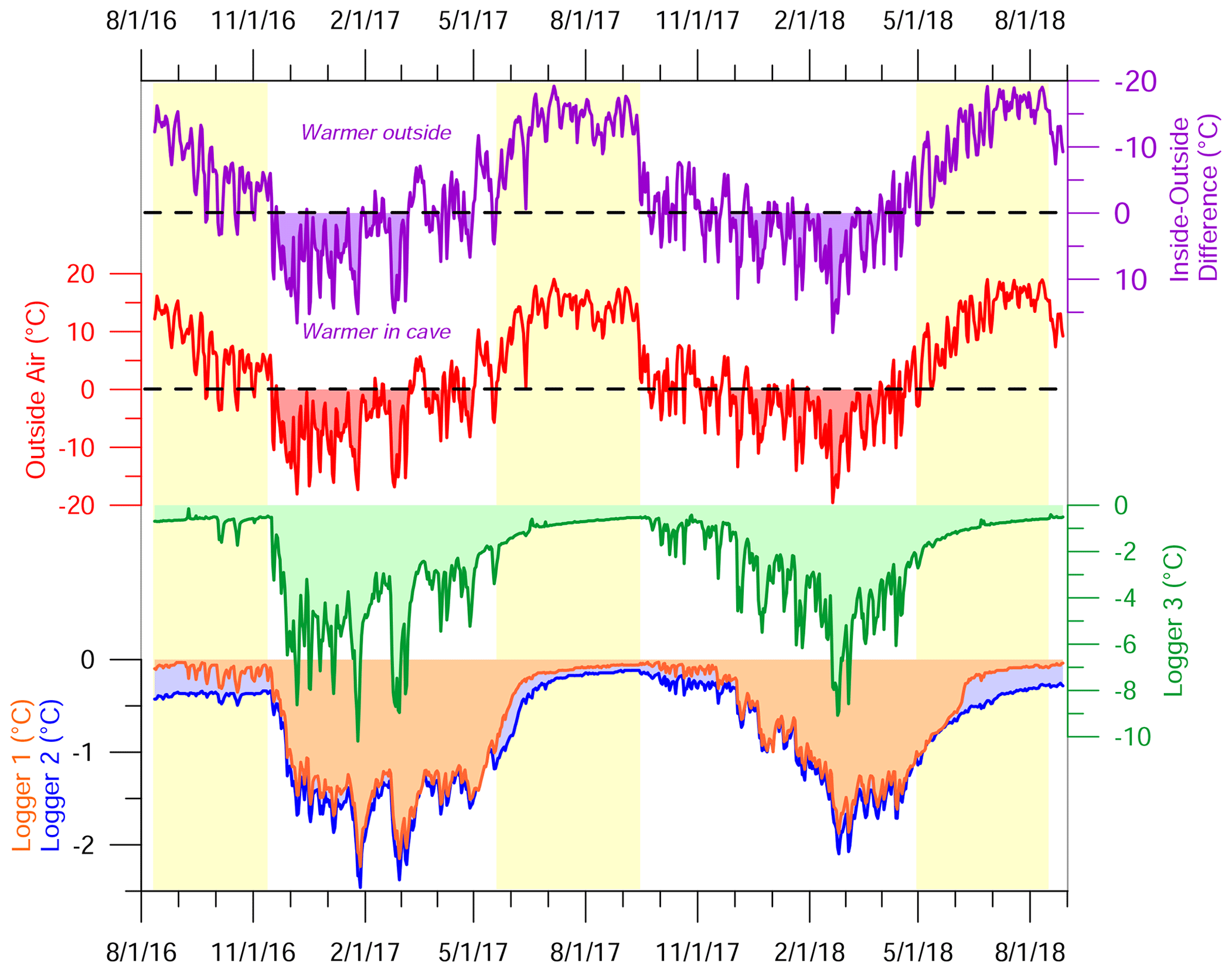
Figure 3Temperature records from data loggers deployed in Winter Wonderland Cave from August 2016 through August 2018. Logger 1 was at the Skating Rink, Logger 2 along the Frozen Freeway, and Logger 3 in the Icicle Room (Fig. 1c). Outside air temperature was recorded by a logger in a solar-radiation shield outside the cave entrance. Yellow shading highlights the summer periods, when cave ventilation is greatly reduced. The purple time series at the top displays the difference between the temperature at Logger 1 and the temperature outside the cave; note the inverted axis. Time series from loggers within the cave are filled below 0 ∘C. Dashed black lines highlight 0 ∘C on the outside air and the temperature difference plots.
The record from the logger outside WWC indicates a mean annual air temperature of 2.3 ∘C (Fig. 4a). The winter of 2016–2017 was colder than 2017–2018 (based on the average temperature between 1 November and 1 May). Both winters had a similar absolute coldest temperature of around −21 ∘C. Winter 2017–2018 had a longer stretch of time between the first and last subzero temperatures, but the beginning of this winter was relatively warm. As a result, winter 2016–2017 recorded 950 freezing degree days (∑(0 ∘C − daily mean)) in comparison with 766 during the winter of 2017–2018 (both calculated from 1 November through the end of May). In response to this difference, the data loggers within the cave were approximately 0.5 ∘C colder on 1 May 2017 relative to 1 May 2018.
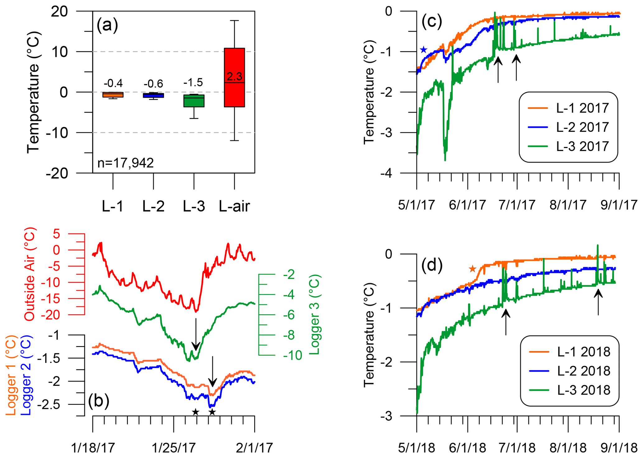
Figure 4Details of temperature records from Winter Wonderland Cave. (a) Box-and-whisker plot showing the distribution of temperature measurements at each of the three loggers (L-1 through L-3) as well as outside the cave. (b) Detailed view of temperature records from late January 2017. A notable low point in temperature outside the cave was mirrored immediately by a temperature drop within the Icicle Room, recorded by Logger 3 on 27 January (star). A corresponding drop in the temperature deeper in the cave was recorded 2 d later (second black arrow and star), supporting the theory that cold air enters through the Icicle Room in winter. (c, d) Temperatures during the summer of 2017 (c) and in the summer of 2018 (d) at the loggers within the cave. The black arrows highlight examples of transient warming in the Icicle Room that were not observed deeper in the cave. The blue star in (c) marks an interval in early May, when the temperature at Logger 2 in the Frozen Freeway briefly rose above the temperature of Logger 1 at the Skating Rink. The orange star in (d) highlights a dramatic, permanent increase in temperature at Logger 1, interpreted to represent the arrival of meltwater at the back of the cave in 2018.
Comparison of the records from all of the loggers indicates that when the outdoor temperature drops significantly below 0 ∘C, the Icicle Room begins to cool, followed a few days later by the loggers deeper within the cave (Fig. 4b). In contrast, once the outdoor temperature stops cycling below 0 ∘C at the beginning of the summer, all loggers within the cave exhibit greatly reduced short-term variability, and temperatures at all of them rise asymptotically toward their equilibrium value, which is reached later in the summer (Fig. 3). Equilibrium temperatures are warmest at Logger 3 (Skating Rink, farthest back in the cave, Fig. 1c) and coldest at Logger 1 in the Icicle Room near the cave entrance (Fig. 3).
Close inspection of the time series also reveals interesting short-term behavior at each of the logger sites. For instance, air temperatures in the Icicle Room (Logger 3) exhibit transient ∼ 1 d increases in air temperature during the summer on several occasions (Fig. 4c and d). These are mirrored by simultaneous but smaller amplitude decreases in temperature at the loggers deeper within the cave (Fig. 4c and d). Notably, after each of these disturbances, temperatures return to their baseline values. Another observation is that in May 2017, the temperature at Logger 2 rose above the temperature at Logger 1 for about 10 d, the only interval during the entire deployment when this reversal occurred (Fig. 4c). Finally, in early June 2018, the temperature at Logger 3 abruptly rose about half a degree and stayed elevated relative to the temperature at Logger 2 for the rest of the summer (Fig. 4d).
3.2 Ground-penetrating radar
GPR surveys along the Frozen Freeway as well as in the Icicle Room provided information about the thickness and internal stratigraphy of the ice. The survey in the Frozen Freeway extended for 75 m through passage of varying widths (Fig. 1c). Because the antenna was shielded, reflections from the cave walls and ceiling were not an issue. However, in the narrowest sections (less than 2 m wide), overlapping reflections from the cave walls beneath the ice surface made it difficult to identify consistent stratigraphy in the ice. Nonetheless, in the 35 m spanning the wider sections, such as the Skating Rink, clear stratigraphic details within the ice are apparent in the radar data (Fig. 5). These take the form of subparallel bands at various depths, which are laterally consistent over several meters. There is a general trend of less pronounced reflectors in shallower parts of the ice, whereas the strongest reflectors are found at depths greater than a meter below the ice surface.
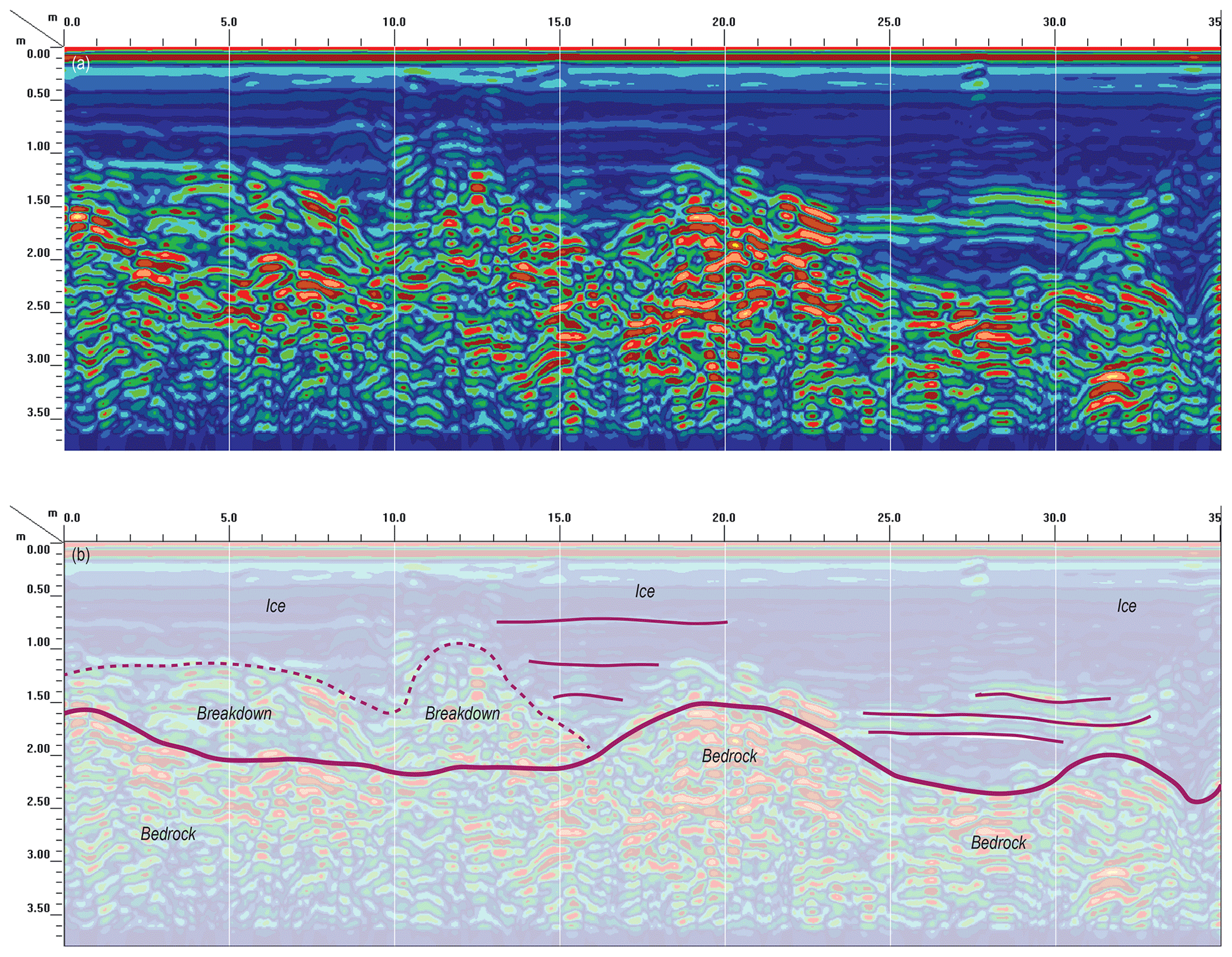
Figure 5Results of a ground-penetrating-radar (GPR) survey along the Frozen Freeway. (a) Uninterpreted GPR data for half of the full survey length (35 m out of 75 m), with the back of the cave on the right. Vertical white lines mark measured points every 5 m used for scaling the GPR survey. (b) Interpretation of the GPR survey shown in (a). The bedrock surface is represented by an irregular but laterally continuous contact. More isolated and discontinuous zones of high-amplitude reflectors above this contactor interpreted as piles of breakdown. Ice beneath the Skating Rink, between 20 and 35 m along the transect, reaches a maximum thickness of nearly 2.5 m. Ice along the Frozen Freeway, between 0 and 20 m, has a maximum thickness of ∼ 2 m. Horizontal lines within the ice are interpreted as stratigraphic layers.
Along the entire length of the Frozen Freeway transect, a continuous reflector is discernible at depth, which likely represents the contact between the ice and the underlying bedrock (Fig. 5). In the Skating Rink, where the cave is widest, and reflections from the walls were not an issue, the maximum depth of this reflector (using a dielectric permittivity of 3.15) is between 2 and 2.5 m below the current ice surface.
The GPR transect in the Icicle Room spanned a length of 8 m. Results imaged layered ice superimposed on a sloping bedrock surface locally mantled by blocks of cave breakdown (Fig. 6). As in the Frozen Freeway, the upper 1 m of this ice exhibits only faint laminations; however below a depth of ∼ 1 m the strength of the reflectors defining these laminations increases markedly. Based on the pattern of these parallel reflectors and their relationship with the sub-adjacent, higher-intensity reflectors from the bedrock, the maximum ice thickness in the Icicle Room, again assuming a dielectric permittivity of 3.15, may exceed 3 m (Fig. 6).
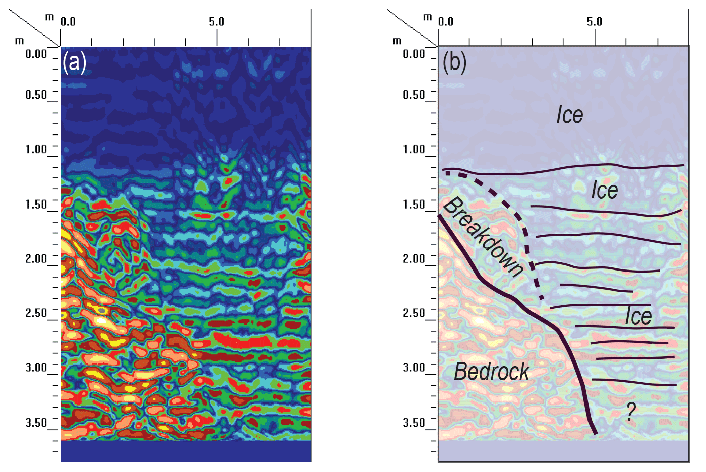
Figure 6Results of an 8 m long ground-penetrating-radar (GPR) survey across the Icicle Room, presenting uninterpreted (a) and interpreted (b) data. From the surface to a depth of ∼ 1 m, the ice is only faintly stratified, whereas below that depth the ice contains increasingly prominent radar reflectors. The steeply sloping bedrock surface is defined on the left side of the transect, mantled in places by breakdown. The maximum thickness of ice here is unclear, but it may be in excess of the 3.5 m penetrated by the 400 MHz GPR system.
3.3 Radiocarbon dating
Seven samples of rodent droppings collected from WWC were submitted for AMS radiocarbon dating. Six of these samples were successfully dated, yielding ages from 40 to 285 radiocarbon years, corresponding to median calibrated ages from CE 1830 to CE 1560 (Table 1, Fig. 7). The oldest of these samples has a 2σ calibration range that extends back to CE 1520. Three of the samples have 2σ calibration ranges that extend, with low probability, into the 20th century (Fig. 7). Overall, the estimated depths of the samples below the local ice surface have no relationship with their ages. The oldest sample (WWC-FF-5) was from the shallowest depth (5 cm). On the other hand, two samples obtained near one another from the same depth (WW-20a and WW-20b) yielded identical ages.
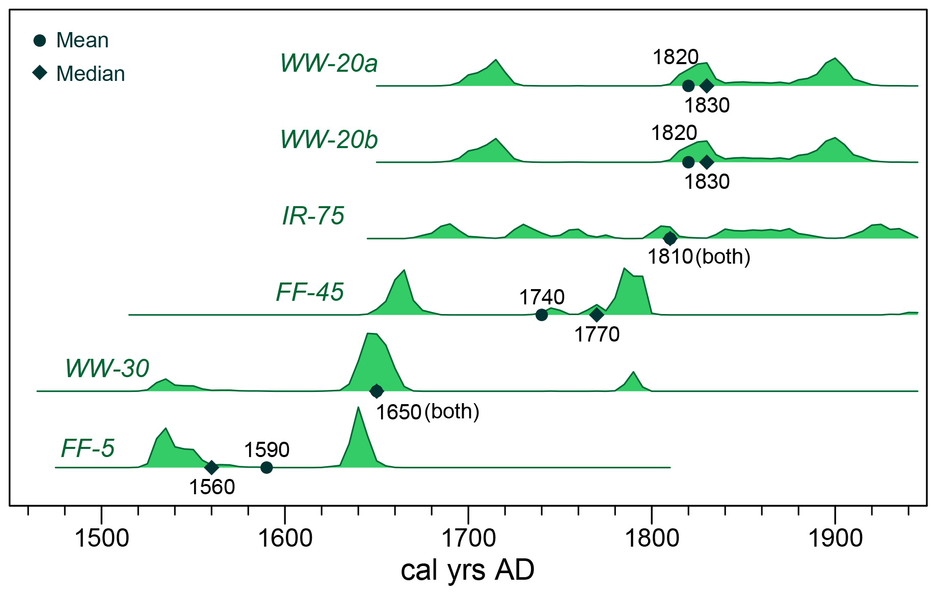
Figure 7Calibration ranges from the IntCal 20 calibration curve for radiocarbon dates obtained from Winter Wonderland Cave. Sample labels correspond with Table 1. Circles mark the mean calibrated age for each sample; diamonds denote the median age. Both are labeled in years CE.
3.4 Stable isotopes
A total of 94 samples collected from the continuous exposure at the back of the Skating Rink (Fig. 2) and from isolated exposures of ice in and near the Icicle Room were analyzed successfully for δ18O and δD. Overall, values of both isotopes are notably depleted relative to VSMOW, with an average δ18O of −14.0 and δD of −104 (Table 2). Minimum and maximum values of δ18O are −17.6 ‰ and −8.7 ‰ and for δD are −125 ‰ and −64 ‰. Overall, values of δ18O and δD are strongly and linearly correlated with one another (r2 of 0.957).
Table 2Stable-isotope results for Winter Wonderland Cave.
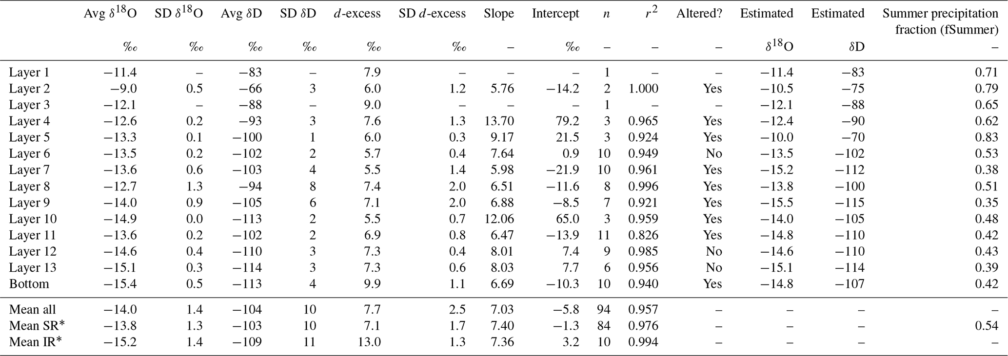
* SR: Skating Rink; IR: Icicle Room. The δ18O and δD estimations were determined from the intersection of the line fit to the data with the meteoric water line
Given the wide range of isotope values in the samples from the Skating Rink exposure, a three-step screening was conducted to identify outliers. First, values of d-excess in parts per thousand were calculated as d-excess =δD − (8×δ18O) (Dansgaard, 1964). Second, because the distribution of the original data was not normal as revealed by a Shapiro–Wilk test (p=0.014), the values were log-transformed. Third, values > 2 standard deviations away from the mean were tagged as outliers. This process identified three samples: two with anomalously low values of d-excess and one with an unusually high value (Fig. 8). These samples were removed from further consideration, leaving 81 samples from this exposure.
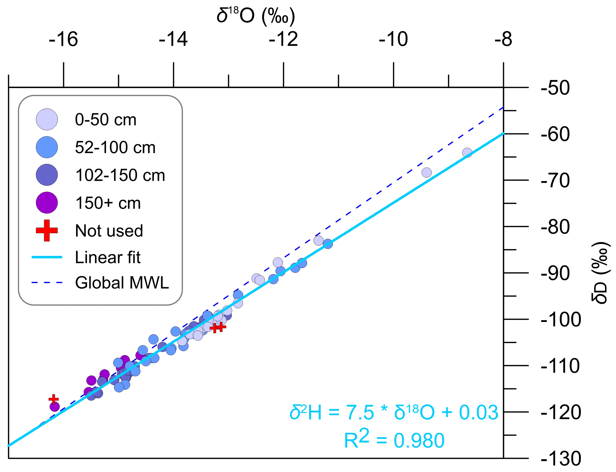
Figure 8Plot of δ18O vs. δD for ice samples from the Skating Rink exposure (Fig. 1c). Samples are color-coded to highlight their depth below the top of the exposure. Three samples identified as outliers and discarded from the dataset are marked with red crosses. The solid light-blue line represents a linear regression through the remaining 81 samples, and the equation for this line is presented in the lower right corner. The dashed blue line is the global meteoric waterline (Craig, 1961).
On a plot of δ18O vs. δD, these 81 samples from the Skating Rink exposure plot parallel to and generally slightly below the global meteoric waterline (Fig. 8). A linear regression through the 81 samples from the continuous exposure has a slope of 7.5 and y intercept of 0.03 (r2 of 0.980).
Plotting values of δ18O and δD vs. depth in the 2 m high exposure reveals short-term variability superimposed over a longer trend (Fig. 9). In general, deeper samples have more negative δ values. Samples with the highest values were collected from within a few centimeters of the cave ceiling. The overall trend in d-excess runs generally contrary to δ18O and δD, with higher values in deeper ice (Fig. 9).
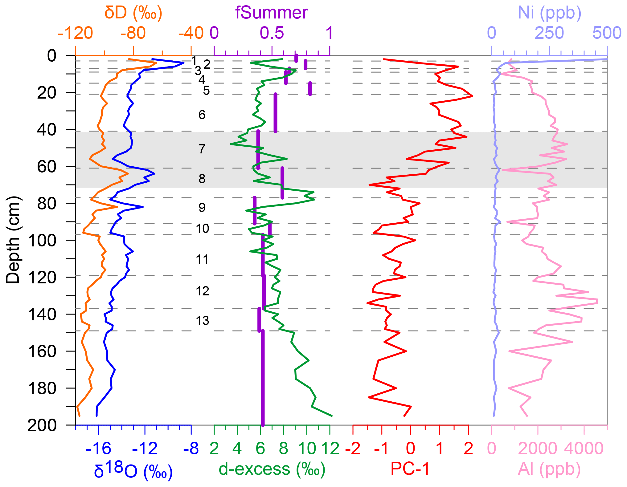
Figure 9Composite plot of values measured in the Skating Rink plot against depth below the top of the exposure. Values of δ18O vs. δD are shown in the first column. The d-excess and the reconstructed fraction of summer monsoonal water in the ice are shown in the second column. The first principal component determined for the glaciochemistry result is displayed in the third column. The two elements which do not fit into PC-1, Al, and Ni are shown in the fourth column. Dashed horizontal lines mark visible boundaries observed in the exposure. From top to bottom, these layers are numbered 1 through 13. The shaded gray region marks the approximate depth from which the radiocarbon ages along the Frozen Freeway were obtained. The ice in this depth range likely dates to between CE 1560 and 1830; deeper ice is older.
In the field, the upper 1.5 m of this exposure, which was more accessible, was visibly stratified, with thin layers of fine carbonate precipitates defining boundaries between 13 discernible layers (Fig. 2). Similar layers were not noticed in the bottom 50 cm of the exposure; however this may reflect the fact that it was difficult to view the bottom of the exposure head-on. Some of these layers, which range from 2 to more than 20 cm thick, correspond with variations in δ18O and δD (Fig. 9). For instance, δ values are notably higher in Layer 2, with δ18O up to −8.7 ‰. Similarly, Layer 8 and the central part of Layer 9 both contain ice with relatively high δ values. However, isotopic values do not always change appreciably across these layer boundaries. For example, δ18O and δD rise steadily through Layer 5, continuing a trend that spans from Layers 4 through 6 (Fig. 9). The boundary between Layers 10 and 11 appears to be the only instance in which a visible boundary coincides with a major change in isotope values (a shift in δ18O of 1.2 ‰ and δD of 12 ‰).
3.5 Glaciochemistry
A total of 13 major and trace elements were detectable in ice samples analyzed from the exposure at the Skating Rink. Ranked in order from most to least abundant they are Ca > Al > Mg > K > Na > P > Si > Ni > Ti > Ba > Sr > Mn > Rb (Fig. 10). Peak abundances of calcium are ∼ 20 000 ppb, and Al, Mg, K, and Na are all detectable in some samples at concentrations above 1000 ppb. Rubidium is the least abundant detectable element, generally with a mean of 0.5 ppb. P, Si, and Sr were not detectable in some samples. A principal component analysis applying a varimax rotation to log-transformed values of Ca, Al, Mg, K, Na, Ti, Ba, Mn, and Rb (removing P, Si, and Sr, which were not detectable in all samples) loads all elements except Al and Ni on the first principal component (PC-1) at values from 0.763 to 0.890. These elements follow a consistent pattern of generally low values in the bottom half of the exposure, rising values between ∼ 100 and 50 cm depth, and notably elevated values in the uppermost 50 cm (Fig. 9). In contrast, Ni exhibits the strongest positive correlation with PC-2 (0.891), and Al is strongly and negatively correlated with PC-3 (−0.827). Nickel has general low and stable values until the uppermost sample, whereas Al abundance is high between 125 and 150 cm and again around a depth of 50 cm (Fig. 9).
Similar elemental abundances were measured in the ice samples collected between the Frozen Freeway and the Icicle Room. Calcium is again the most abundant element, with an average concentration of 4850 ppm, and Rb is the least abundant (< 1 ppm). Mean abundances for all elements in these samples are strongly correlated with those measured for the Skating Rink exposure (r2 of 0.945). Unlike in the exposure at the Skating Rink, there is no obvious trend in abundance in these samples. However, because they were collected from isolated locations where ice was locally visible between blocks of breakdown, their relationship with one another is unclear, and it may be inappropriate to consider them parts of a stratigraphic sequence.
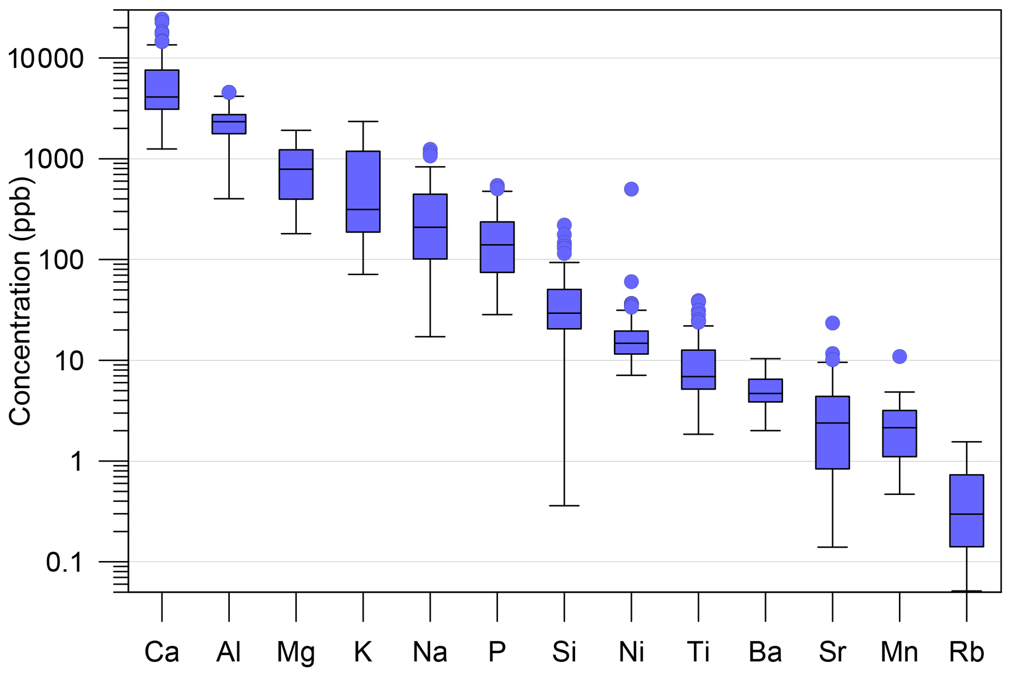
Figure 10Box-and-whisker plot presenting the abundance of detectable elements in samples from the Skating Rink exposure, arranged from most to least abundant. Central lines represent median values, boxes represent interquartile range, whiskers represent interquartile range ×1.5, and circles represent outliers.
4.1 Origin, extent, and age of the ice
The data loggers that recorded air temperatures between 2016 and 2018 provide a clear explanation for why perennial subzero conditions are maintained inside WWC despite a mean annual temperature of +2.3 ∘C outside the entrance. As illustrated in Fig. 3, cold air enters the Icicle Room (Logger 3) whenever the outside air temperature drops notably below the temperature in the cave. If cold temperatures outside are maintained for more than a few days, this cold pulse penetrates deep enough into the cave to be recorded by Logger 2 in the Frozen Freeway and Logger 1 at the Skating Rink (Fig. 4b). Although the slight downhill slope of the entrance passage leading to the main part of the cave would alone encourage the entry of dense cold air in winter, the extreme narrowness of the actual cave entrance (< 25 cm) combined with the observation of a substantial draft flowing through the cave during each field visit suggests that a connection exists between the currently accessible end of WWC and the surface of the plateau ∼ 100 m above the cave. This conduit acts as a chimney, allowing relatively warm air within the cave to rise towards the surface in the winter (Balch, 1900; Luetscher and Jeannin, 2004b; Thury, 1861). This air is replaced by cold air flowing in through the cave entrance into the Icicle Room, refrigerating the cave interior throughout the winter. In contrast, during the summer, there is a minor reversal of this pattern as cold air within the cave flows out through the entrance, replaced by warm air penetrating downward through the hypothesized connection between the cave and the plateau surface. However, because the entrance of the cave is ∼ 15 m higher than the Frozen Freeway (Fig. 1c), it is not possible for all of the dense cold air to be evacuated from the cave in the summer. As a result, the interior of WWC is disproportionately impacted by cold air in winter and is relatively unaffected by summer warmth.
Occasionally, during the summer months the temperature in the Icicle Room abruptly jumps ∼ 1 ∘C before returning to baseline levels (Fig. 4c and d). This shift is accompanied by a minor temperature decrease at the loggers deeper in the cave. This pattern indicates that some process brings relatively warm outside air into the Icicle Room, displacing colder air deeper into the cave but not for long enough to have a lasting impact on the overall temperature distribution. Comparison of the logger records with meteorological data from the Chepeta RAWS (remote automated weather station) 60 km to the east (Fig. 1b) at a slightly higher elevation (3680 m) indicates that each of these transient temperature increases was associated with wind from 320 to 340∘ at velocities greater than 15 m/s. Given the orientation of the cave entrance, this azimuth is perfectly aligned to push relatively warm outside air through the cave entrance, temporarily warming the Icicle Room and displacing cold air deeper into the cave. However, because the general airflow is outward during the summer, as soon as the wind direction or velocity changes, and warm air is no longer forced into the cave, the pattern reverses, and the Icicle Room cools down again.
Given the distribution of ice and the lack of ice stalactites or stalagmites along the Frozen Freeway, it appears that the water responsible for the ice in WWC entered through the boulder-choked constrictions in the rear of the cave as well as through the entrance into the Icicle Room. Because there are no streams or lakes in the landscape above the cave, this water is likely derived from infiltrating precipitation. Furthermore, given the climate at this location, much of this water is likely related to the melting of winter snowpack in late spring. This rapid melt produces a pulse of water that penetrates downward through the epikarst to reach the back of the cave, perhaps following the conduit that allows cave air to rise toward the surface in the winter. Snowmelt on the north-facing cliff above the cave entrance can enter the Icicle Room directly. It is also possible that intense summer rainstorms may deliver water to the plateau above WWC in quantities sufficient to reach the cave. Either way, this water freezes upon entering the subzero cave interior, incrementally adding a new layer to the perennial ice deposit. Given the hypothesized conduit linking the cave to the surface, this model of ventilation for maintenance of freezing temperatures, and the apparent formation of ice from inflowing water, WWC can be classified as a “dynamic cave with congelation ice” (Luetscher and Jeannin, 2004a).
Winter Wonderland Cave was not visited during the summer of 2017, so it is unknown whether water entered the cave that year. However, in August 2018, liquid water and new ice were noticed at the Skating Rink and along parts of the Frozen Freeway. The temperature data logger from the Skating Rink (Logger 1) recorded a ∼ 1 ∘C increase in temperature during the first week of June 2018 (Fig. 4d). In contrast to the summer temperature increases in the Icicle Room, this temperature rise was long-lasting: during the weeks leading up to this point the temperatures at Logger 1 and Logger 2 were identical, yet after this point, Logger 1 at the Skating Rink remained ∼ 1 ∘C warmer than Logger 2. The arrival of relatively warm meltwater to the back of the cave at this time could explain the abruptness of this temperature jump, and the slow release of latent heat as this water froze could have maintained the slightly warmer temperatures relative to Logger 2. Snowpack-monitoring sites at Trial Lake and Brown Duck, at similar locations, elsewhere in the southwestern Uinta Mountains (Fig. 1b) rapidly lost the majority of their snow water equivalent in May 2018. This offset suggests that it requires ∼ 1–2 weeks for meltwater to transit from the plateau surface to the cave.
Results from the GPR surveys indicate that the ice forming the floor of the Frozen Freeway is generally from 1 to ∼ 2.5 m thick and has accumulated over an uneven surface of bedrock and blocks of breakdown (Fig. 5). The 2 m high exposure of ice at the edge of the Skating Rink starts ∼ 45 cm above the floor of the Frozen Freeway, exploiting remnant ice layers reaching to the cave ceiling that have not been removed by sublimation (Fig. 2). Given the assumed dielectric permittivity, therefore, it is possible that as much as a meter of additional ice exists below the deepest stratigraphic level accessible in this exposure. Similarly, in the Icicle Room, an ice thickness possibly in excess of 3 m was imaged (Fig. 6). In both locations, the tendency of the upper ∼ 1 m of ice to exhibit reduced stratigraphic layering compared with the deeper ice may reflect a greater presence of mineral precipitates, dust, or organic matter concentrated at specific levels within the deeper ice.
Determining the age of cave ice deposit is rarely straightforward, and the situation in WWC is no different. Compared with a sag-type cave in which snow and organic matter accumulate in a vertical shaft (e.g., Munroe et al., 2018; Spötl et al., 2014), the interior of WWC is relatively devoid of organic matter. On the other hand, the radiocarbon-dated rodent droppings do provide important age constraints (Fig. 7). Because these samples were collected from the upper layers of the ice deposit (Fig. 2), they provide minimum limits on the age of the ice, suggesting that most of the ice accumulated before ∼ CE 1830.
4.2 Paleoclimate implications
The overall pattern in these data is that the deep ice is more depleted in heavy isotopes relative to VSMOW, whereas stratigraphically higher ice is less depleted (Fig. 9). This trend indicates a long-term change in the isotopic composition of the water entering WWC. Air temperature exerts a well-documented effect on isotopic values of precipitation, with a lower temperature of condensation corresponding to lower values of δ18O and δD (Dansgaard, 1964). Therefore, one possible interpretation is that average air temperatures increased over the time period represented by the Skating Rink exposure. However, given the relationship between monthly average temperature and estimated δ18O for precipitation at the Brown Duck snowpack telemetry (SNOTEL) site (Fig. 1b), the difference between the lowest (−16.2 ‰) and highest δ values (−8 ‰) in samples from this exposure would correspond to a temperature change of approximately 11 ∘C. This result exceeds the temperature difference between full-glacial and modern conditions in the Uinta and Wasatch mountains determined from numerical modeling of paleoglaciers (Laabs et al., 2006; Quirk et al., 2018, 2020). It is difficult to imagine that the ice in WWC is residual from the last glaciation, which reached its maximum in this area at 18–20 ka (Laabs et al., 2009; Quirk et al., 2020); thus the measured changes in the isotopic values are unlikely to be solely a function of temperature.
A more plausible interpretation is that the isotopic variability reflects changes in the relative abundance of seasonal precipitation over WWC. Under the modern climate, the Uinta Mountains are influenced by two distinct precipitation patterns strongly linked to specific seasons. Storms penetrating inland from the Pacific Ocean produce a peak of precipitation during December, January, and February (Mitchell, 1976). By virtue of the cold winter air temperatures and the long transport pathway for this moisture passing over multiple mountain ranges, this precipitation has notably low δ18O and δD values. In contrast, during the summer, primarily in August, moisture with relatively higher isotopic values is delivered from the south by the North American Monsoon circulation (Metcalfe et al., 2015; Ropelewski et al., 2005). Correspondingly, the Online Isotopes in Precipitation Calculator predicts that the location of Winter Wonderland Cave receives precipitation with δ18O around −23 ‰ in winter and around −8 ‰ in August.
The rapid 1 ∘C increase in air temperature recorded by the logger at the Skating Rink in early June 2018 is a likely signal for the arrival of snowmelt at the beginning of that summer (Fig. 4d). However, liquid water was still present at the Skating Rink more than 2 months later on 29 August 2018. Similarly, although there is no temperature record for the summer of 2019, liquid water was again observed at the Skating Rink on 19 August 2019. Assuming that the meltwater pulse usually arrives at the beginning of the summer, matching the annual timing of snowmelt, the persistence of a thin layer (centimeter-scale) of liquid water in subzero conditions for multiple months is improbable. Therefore it is likely that additional water entered the cave later in the summers of 2018 and 2019, after the main snowmelt pulse. This summer water would most conceivably reflect the monsoonal precipitation that dominates in August. In this model, therefore, the water forming ice in WWC represents an integrated snowpack signal that is augmented by some amount of isotopically heavier summer precipitation.
The isotopic composition of the snowmelt directly above WWC is unknown. However, fully integrated snowpack samples collected at the elevation of the plateau above the cave at Pole Mountain ∼ 50 km eastward along the southern flank of the Uinta Mountains in late March 2019 had an average δ18O of −18.9 ‰ (Fig. 1b). Similar full-snowpack samples collected at the same elevation in early April 2019 at Trial Lake ∼ 25 km northwest of WWC had an average δ18O of −20.3 ‰ (Fig. 1b). The mean of all these values (−19.6 ‰) is lower than the value of −18.2 ‰ for two samples of water collected from the Skating Rink surface in August 2019, indicating that the water collected in the cave that summer was a mixture of winter snowmelt and isotopically heavier summer rain.
With this insight, a linear mixing model was constructed to predict the δ18O value of water comprised of varying proportions of two end-members: snowmelt (at −19.6 ‰) and monsoonal rain (−8 ‰). This model suggests that the water collected from pools on the surface of the Skating Rink in late summer 2019 was a mixture of 88 % winter snowmelt and 12 % summer rain. This estimate of the summer component in this sample is a minimum because the water had already begun to freeze beneath a lid of ice, which would drive δ18O in a more negative direction in the remaining water (Jouzel and Souchez, 1982; Perşoiu et al., 2011). Nonetheless, the value of δ18O in the modern water is more negative than any of the analyzed ice samples, indicating either that this water contained a lower fraction of summer rain than the ice samples or that the snowmelt pulse in 2019 was unusually large.
Applying this mixing model to the ice samples requires an assessment of whether the isotope values in the ice reflect those of the original precipitation or if they have been altered during freezing. In this regard it is notable that the ice in WWC is seen in vertical exposures to consist of visually distinct layers from < 5 to ∼ 20 cm thick, delineated by mineral precipitates and changes in bubble density (Fig. 2). Layering on a similar scale is also resolvable in the GPR results (Figs. 5 and 6). If these layers were constructed through the incremental additions of thin films of water, then the mineral precipitates defining the visible layer boundaries could have formed in response to sublimation that lowered the ice surface, creating a lag of material that was originally included in the ice. Alternatively, the visible layers may have formed through slow, closed-system freezing of pools of water with a depth equivalent to the resulting layer thickness. Mineral precipitates would have formed within each pool as the floating ice thickened downward, concentrating the residual liquid water. Ice formed by these two mechanisms are termed “floor ice” and “lake ice”, respectively (Perşoiu et al., 2011).
Downward freezing of a layer of water beneath a thickening lid of ice will result in ice that is sequentially more depleted in heavy isotopes at depth as the heavier 18O and deuterium are preferentially incorporated into the early-formed ice at the surface (Citterio et al., 2004b; Persoiu and Pazdur, 2011; Souchez and Jouzel, 1984). Thus, plotting δ18O and δD vs. depth and highlighting the locations of visually identified layer boundaries were employed to determine the likely origin of the different ice layers. When plotted this way (Fig. 9), several layers exhibit trends of increasing isotope depletion with depth; however these differences are generally < 1 ‰ for δ18O from top to bottom in a given layer. The exception is Layer 8, where δ18O falls from −12 ‰ to −15 ‰ over a layer thickness of 14 cm. Previous work has shown that a top-to-bottom offset in δ18O of ∼ 4 ‰ occurs within 5 to 10 cm thick layers of lake ice in a well-studied Romanian ice cave (Perşoiu et al., 2011; Perşoiu and Pazdur, 2011). With this observation as a reference point, Layer 8 in WWC likely formed through closed-system freezing of a thick layer of water, and it is possible that this process slightly impacted some other layers as well.
Another way to evaluate the likelihood that ice formed through closed- or open-system freezing is to plot δ18O vs. δD from an individual layer and assess whether the values align with the (local) meteoric waterline, indicating floor ice, or with a lower “freezing slope”, indicative of more extensive fractionation, typical of lake ice (Jouzel and Souchez, 1982; Perşoiu et al., 2011). When arranged this way, sets of samples (n≥3) defining individual layers in the Skating Rink exposure have slopes from 6.0 to 13.7 (Table 2). Layers 6, 12, and 13 have slopes that are close to the meteoric waterline. The isotopic measurements in these layers, therefore, likely record the composition of the original meltwater with fidelity. In contrast, Layers 7, 9, and 11 and the bottom ice have lower slopes, suggesting more extensive fractionation during freezing. The slopes of Layers 4, 5, and 10 are quite high (> 9), although they were determined for just three points. Previous work has demonstrated that isotopic composition of the original water can be found at the intersection of a line fit to the δ18O and δD measurements for an individual ice layer and the meteoric waterline (Jouzel and Souchez, 1982; Perşoiu et al., 2011). Applying this approach yields estimates of original δ18O and δD values for the layers that appear to have fractionated extensively during closed-system freezing (Table 2).
Two cautions must be noted when considering this analysis. First, samples were not collected continuously through the exposure; they were spaced 2 cm (for the upper part) and 5 cm (for the lower part) apart. As a result, not all ice was sampled, and the isotopic composition of the ultimate top and bottom ice in a given layer is unknown. Second, previous work has noted that kinetic effects during rapid freezing can cause deviations from the freezing slope (Perşoiu et al., 2011). Based on relationships between δD and d-excess, kinetic effects likely played a role in the formation of at least some layers in the Skating Rink exposure. Nonetheless, with these considerations in mind, estimated isotopic compositions of the original water obtained from the intersection of the freezing slope and meteoric waterline were combined with the average isotopic values for layers that apparently did not fractionate greatly, based on downward trends in isotope values and δ18O vs. δD slopes.
Applying the mixing model presented earlier to the average (measured and reconstructed) values of δ18O for ice layers in the Skating Rink exposure suggests that the deepest, oldest ice formed from water containing ∼ 40 % summer precipitation (fSummer, ∼ 0.40) and that the fraction of monsoonal moisture increased to ≥ 60 % near the top of the exposure (Fig. 9). Two outliers to this pattern are notable: a peak value of 83 % in Layer 5 and a lower value of 38 % in Layer 7. However, Layer 5 was thin and is represented by just three data points, creating uncertainty in its regression slope that carries over into the estimate of original water composition. Layer 7 contains two sets of isotopic values, a constant upper half and a lower half with a pronounced negative excursion (Fig. 9), implying that the suite of samples collected may have inadvertently spanned two layers separated by a contact that went unnoticed in the field. An obvious limitation is that this simple model assumes that the isotopic composition of snowmelt and monsoonal precipitation was constant over time. It also assumes that the interpolated isotopic value for August precipitation from the OPIC is accurate and that the snowpack samples from 2019 adequately represent the composition of the snow on the plateau above WWC. Nonetheless, even with these considerations, it is notable that the relative importance of winter and summer precipitation appears to have changed at this location over time.
The radiocarbon-dated organic remains were collected within the uppermost layers of ice forming the floor of the Frozen Freeway, which corresponds to Layers 7 and 8 in the Skating Rink exposure (Figs. 2 and 9). This relationship allows the exposure to be divided broadly into a lower part, where the ice apparently accumulated prior to the 1800s, and an upper part (Layers 1 through 6), which accumulated more recently. The lower layers, therefore, correspond with the interval of generally cooler temperatures in the Northern Hemisphere referred to as the Little Ice Age (Grove, 1988). The reconstructed summer water content of this ice varied in a narrow range between 40 % and 50 %, suggesting relatively consistent conditions under which the snowmelt pulse and summer monsoon contributed roughly equal amounts of water to the cave. After this time, summer water began to exert a greater control over the isotopic composition of the ice.
Records of δ18O from lake sediments on the White River Plateau in northwestern Colorado (Fig. 1a) suggest that winters during the Little Ice Age were notably snowy, with snowfall making up the greatest fraction of annual precipitation at any time during the Holocene (Anderson, 2012). After that time, snowfall became less important. A similar pattern is seen in multiproxy lacustrine records from San Luis Lake (Fig. 1a) in southern Colorado (Yuan et al., 2013). The suggestion that water derived from the melting of winter snow contributed to a greater fraction of the ice forming in WWC during the Little Ice Age is consistent with these other regional hydroclimate records. An additional point of reference is provided by isotope measurements in a glacier ice core from the Wind River Mountains (Fig. 1a), ∼ 400 km to the northeast of WWC (Naftz et al., 1996). In that core, a positive shift in δ18O of ∼ 1 ‰ accompanied the end of the Little Ice Age around CE 1845 (Schuster et al., 2000). The magnitude of this shift is about half as large as the change in δ18O between the bottom of Layer 6 and the top of the Skating Rink exposure (excluding the unusually enriched samples from Layer 2). Part of the trend toward higher δ18O values in the uppermost part of the Skating Rink exposure may, therefore, reflect an increase in average air temperature as the Little Ice Age ended.
4.3 Glaciochemistry interpretation
The elemental abundances measured in the ice from WWC are generally similar from sample to sample, suggesting that the composition of the water did not change dramatically over time. Such constancy fits the assumption that the majority of the dissolved load in the water was obtained through water–rock dissolution reactions in the epikarst. If the pathways leading water from the plateau surface down to the cave did not change appreciably over the time period represented by the ice, then it is logical that the overall chemical signature of this ice was relatively constant.
At the same time, however, the majority of elements exhibit a notable increase in concentration in the upper part of the ice. This pattern is consistent across nearly every detectable element and is clearly seen in the first principal component (PC-1) calculated from these elemental abundances (Fig. 9). The shift toward greater elemental enrichment occurred primarily as a step change in Layer 8, which as noted above contains organic remains dating to the latter part of the Little Ice Age. Thus it seems that the glaciochemical composition of this ice changed between the Little Ice Age and the years that followed. Consideration of the setting of WWC and available information about regional hydroclimate in the latest Holocene reveals possible explanations for the rising elemental abundances in the younger ice. First, the decrease in winter snowpack after the Little Ice Age noted in the lacustrine records (Fig. 1a) from Colorado (Anderson, 2012; Yuan et al., 2013) could have slowed the rate of infiltration through the epikarst, affording water a longer contact time with host rock during transit from the ground surface to the cave, leading to an increased dissolved load in the water. Furthermore, if a greater fraction of the water reaching the cave was coming from summer monsoonal moisture rather than winter snowmelt, near-surface rock temperatures in the epikarst may have been elevated above Little Ice Age values, increasing rates of dissolution reactions. Either way, the increase in dissolved load in the ice roughly at the same time as the shift toward an apparently higher fraction of summer moisture, along with an overall decrease in the observed thickness of the ice layers, is consistent with a shift toward reduced winter snowfall.
One element that notably does not follow the pattern of increasing abundance in the uppermost ice is Al, which is most abundant in samples from Layer 12 and Layer 7 (Fig. 9). Aluminum is not present in significant quantities in the carbonate bedrock hosting WWC, suggesting that the Al in the ice has another source. Previous work has documented the abundance of Al in Uinta Mountain dust, where Al in the form of aluminosilicates is present at a weight percent abundance of ∼ 7 % (Munroe, 2014). Thus the changing abundance of Al in the Skating Rink exposure may reflect variations in the abundance of dust brought into the cave by inflowing air currents during winter. This raises the possibility that additional age control, combined with the collection of more ice samples, could allow reconstruction of dust abundance over time from this layered ice deposit.
A final observation in the glaciochemistry is the greatly elevated level of Ni in the uppermost samples. After averaging 16.5 ppb through nearly all of the Skating Rink exposure, Ni rises in the uppermost 10 cm and reaches a maximum of 500 ppb in the youngest sample immediately below the cave ceiling (Fig. 9) Work elsewhere in the Uinta Mountains has demonstrated that the abundance of Ni is elevated in modern dust (Munroe, 2014) as well as in lake sediments that accumulated after CE 1900 (Reynolds et al., 2010). This dramatic increase in Ni abundance has been ascribed to fugitive dust from mine tailings and other anthropogenic activities in the southwestern US. In WWC, the increase in Ni levels begins to rise in ice approximately 30 cm stratigraphically higher than the radiocarbon ages (Fig. 9), a relationship that adds further support for the theory that the uppermost ice accumulated after the Little Ice Age.
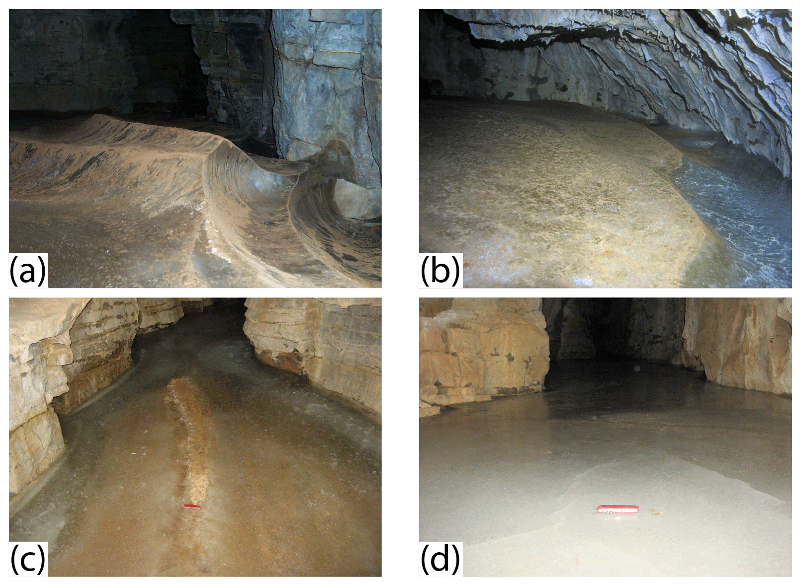
Figure 11A selection of photographs highlighting changes observed in Winter Wonderland Cave. (a) The sculpted surface of the ice along the Frozen Freeway in 2016 illustrating numerous intersecting cuspate forms produced by sublimating air currents. The total relief is ∼ 30 cm. The orange material on the ice is cryogenic-mineral precipitates. (b) A view showing the edge of the ice in the Skating Rink in 2016, where a ∼ 20 cm deep moat had formed at the contact with the rock wall of the cave. (c) The surface of the Frozen Freeway in 2018 illustrating how inflowing water had submerged nearly all of the former sculpted surface under new ice. The red Swiss Army knife is located at the end of a ∼ 1 m long section of the former crest in the ice that still reaches above the new ice surface. (d) Another view from a section of the Frozen Freeway in 2018, where new ice formed from inflowing water has completely inundated the former sculpted ice surface. The red pocket knife is 10 cm long.
4.4 Indications of recent change
Studies of other ice caves have reached the sobering conclusion that many subterranean ice bodies have a negative mass balance and are rapidly disappearing as a direct or lagged response to climate change above the cave (Kern and Perşoiu, 2013; Pflitsch et al., 2016). Winter Wonderland Cave was discovered less than 10 years ago and has only been entered 5 times; thus the period and number of observations is minimal. However, these repeat visits have identified notable evidence suggesting that conditions within the cave have recently changed. During summer visits in 2014, 2015, and 2016 the surface of the ice along the Frozen Freeway was dramatically sculpted into a series of ridges and furrows presumably created by sublimation induced by air currents (Fig. 11a and b). The surface of this ice was mantled by cryogenic-mineral precipitates, and no liquid water was observed anywhere in the cave. The overall impression was that it had been many years since water entered the cave and added a new layer to the ice deposit. Short-term observations of an ice cave in the Canadian Rockies suggest that sublimation producing sculpted patterns on the surface of ice proceeds at a rate on the order of 3 mm/yr (Marshall and Brown, 1974). Thus, the ∼ 30 cm of relief on the surface of the Frozen Freeway suggests that liquid water had not entered the cave for possibly as long as 100 years. As noted earlier, that situation changed dramatically in 2018 and again in 2019, when considerable water entered from the rear of the cave and flooded across the Frozen Freeway, filling most of the troughs and submerging most of the crests (Fig. 11c and d). Certainly, infiltration of liquid water is not a new occurrence in WWC; it is exactly this process which created the layered ice deposit in the first place. On the other hand, the abrupt appearance of this water in 2018 following an apparently long stretch of time in which water failed to reach the cave suggests a significant shift in the availability of water or the thermal environment within the cave. Neither the water years 2017–2018 nor 2018–2019 featured unusual amounts of precipitation, but temperatures at the Brown Duck snowpack-monitoring site (Fig. 1b) have risen at a rate of 0.8 ∘C/decade over the past 25 years. Thus, it is possible that warming temperatures have crossed a threshold and begun to melt ice farther back in an inaccessible part of the cave, contributing to the meltwater observed in the Skating Rink in the last two summers. Melting of ice with more negative isotope values could also explain why the water collected in 2019 had such low values of δ18O and δD.
4.5 Limitations and direction for future research
This multidisciplinary investigation of the perennial ice in Winter Wonderland Cave supports a model for the origin of the ice, provides constraints on the age of the ice, and uses isotopic and glaciochemical data to explore the possible paleoclimate significance of this ice. Despite these achievements, this work remains a preliminary assessment, and there are a number of significant directions in which future efforts could be focused. Foremost among these would be the acquisition of additional age control. The collection and radiocarbon dating of organic remains from other locations within the cave would be helpful in further limiting the age of the ice. Similarly, although uranium abundance was not assessed in the glaciochemistry reported here, it may be possible to directly date the ice with U–Th techniques (Cheng et al., 2013).
In terms of sampling, it may be worthwhile to attempt to retrieve a core where the GPR analysis indicates a maximum ice thickness. Given the difficult access to the cave and a challenging working environment, retrieval of such a core would not be a simple process. However, an ice core would allow the analysis of truly contiguous samples from an unambiguous stratigraphic context. Additional environmental proxies in the ice, for instance pollen (Feurdean et al., 2011), black carbon, or dust, could be studied in a core to reveal more details about environmental conditions outside of the cave when the ice was accumulating.
Either combined with coring or through a separate sampling campaign, it would also be useful to retrieve intact, oriented blocks of ice for crystallographic study (Holmlund et al., 2005). Analysis of crystal orientations, bubble trails, inclusions, and other features would provide information about the conditions under which the ice formed (Citterio et al., 2004a; Marshall and Brown, 1974). Such evidence could be useful in distinguishing between open- and closed-system models for the genesis of the ice layers.
Additional data loggers could be deployed throughout the cave to further collect micrometeorological data. Relative humidity loggers were installed in the cave in 2019 and should be useful in identifying changes in the direction of cave ventilation. Such efforts could be combined with deployment of a three-dimensional, ultrasonic anemometer (Pflitsch and Piasecki, 2003). More data loggers from the rear of the cave might be able to better identify the thermal pulse associated with the arrival of meltwater in early summer. Similarly, deployment of a thermal camera could further document the arrival of this water (Berenguer-Sempere et al., 2014).
Finally, in terms of more traditional cave research techniques, a focused campaign to collect summer precipitation and winter snow on the plateau above WWC would constrain the initial properties of the infiltrating water and permit more nuanced interpretations of the source for the ice and its dissolved load (Carey et al., 2019; Herman, 2019). Similarly, speleothems are present in the cave. None of them are currently active, and no drip water was observed during any of the August visits. However, it would be interesting to determine when these speleothems grew and what they may contain as a paleoclimate record.
Winter Wonderland Cave is a solution cave in Carboniferous limestone at an elevation of approximately 3140 m in the Uinta Mountains of northeastern Utah, USA. The cave contains a layered perennial ice deposit formed by freezing of infiltrating water. Radiocarbon dating of organic remains indicates at least some of this ice accumulated before approximately CE 1830. Ground-penetrating radar indicates that the ice is locally ∼ 3 m thick. Isotopic analysis suggests that some ice layers may have formed during closed-system freezing; however most samples plot near the meteoric waterline. The ice seems to have been formed from a mixture of winter snowmelt and summer precipitation, with winter water dominating in the early part of the record and summer water becoming more significant in the latter part. This shift is consistent with other regional hydroclimate evidence suggesting that winters were unusually snowy during the Little Ice Age. Glaciochemical data indicate that the overall dissolved load in the ice increased after the Little Ice Age. This change may be a sign of reduced rate of infiltration that increased water–rock interaction time. Abundances of Al and Ni follow a different pattern and likely reflect variation in the amount of eolian dust incorporated in the ice over time. The appearance of liquid water in the cave in the last two summers is unusual and may be a sign of a recent change in the cave environment. Collectively these results emphasize the potential significance of the ice in Winter Wonderland Cave as a paleoclimate record and highlight its vulnerability. Future work should focus on acquiring additional age control for this ice and possibly retrieving a continuous core through the ice deposit.
Data generated in this project and not presented in the tables accompanying this paper are available in the HydroShare repository at https://doi.org/10.4211/hs.b5f0000096174af9af94fe62bd2065d6 (Munroe, 2021).
The author confirms sole responsibility for the following: study conception and design, data collection, analysis and interpretation of results, and manuscript preparation.
The author declares that there is no conflict of interest.
David Herron (USDA Forest Service) discovered Winter Wonderland Cave and provided the detailed mapping from which Fig. 1 was simplified. Middlebury students Quinn Brencher, Kristin Kimble, Miranda Seixas, and Caleb Walcott were instrumental in the success of this challenging fieldwork. Thanks to Greg Carling and Kevin Rey at Brigham Young University for assistance with snow collection and the stable-isotope measurements and to Pete Ryan and Jody Smith at Middlebury College for help with the ICP-MS analysis.
This paper was edited by Christian Hauck and reviewed by Aurel Perşoiu and Marc Luetscher.
Anderson, L.: Rocky Mountain hydroclimate: Holocene variability and the role of insolation, ENSO, and the North American Monsoon, Global Planet. Change, 92/93, 198–208, https://doi.org/10.1016/j.gloplacha.2012.05.012, 2012.
Balch, E. S.: Glacieres, or Freezing Caverns, Allen Lane and Scott, Philadelphia, USA, 1900.
Behm, M. and Hausmann, H.: Eisdickenmessungen in alpinen Höhlen mit Georadar, Die Höhle, 58, 3–11, 2007.
Berenguer-Sempere, F., Gómez-Lende, M., Seranno, E., and de Sanjosé-Blasco, J. J.: Orthothermographies and 3D modeling as potential tools in ice caves studies: the Peña Castil Ice Cave (Picos de Europa, Northern Spain), Int. J. Speleol., 43, 35–43, https://doi.org/10.5038/1827-806X.43.1.4, 2014.
Bryant, B.: Geologic and structure maps of the Salt Lake City 1 x 2 quadrangle, Utah and Wyoming, US Geological Survey, Map Number I-1944, 1992.
Carey, A. E., Zorn, M., Tičar, J., Lipar, M., Komac, B., Welch, S. A., Smith, D. F., and Lyons, W. B.: Glaciochemistry of Cave Ice: Paradana and Snežna Caves, Slovenia, Geosciences, 9, 94, https://doi.org/10.3390/geosciences9020094, 2019.
Cheng, H., Edwards, R. L., Shen, C.-C., Polyak, V. J., Asmerom, Y., Woodhead, J., Hellstrom, J., Wang, Y., Kong, X., Spötl, C., Wang, X., and Alexander Jr., E. C.: Improvements in 230Th dating, 230Th and 234U half-life values, and U-Th isotopic measurements by multi-collector inductively coupled plasma mass spectrometry, Earth Planet. Sci. Lett., 371, 82–91, 2013.
Citterio, M., Turri, S., Bini, A., Maggi, V., Pelfini, M., Pini, R., Ravazzi, C., Santilli, M., Stenni, B., and Udisti, R.: Multidisciplinary approach to the study of the Lo Lc 1650 “Abisso sul Margine dell'Alto Bregai” ice cave (Lecco, Italy), Theor. Appl. Karstol., 17, 45–50, 2004a.
Citterio, M., Turri, S., Bini, A., and Maggi, V.: Observed trends in the chemical composition, δ18O and crystal sizes vs. depth in the first ice core from the “LoLc 1650 Abisso sul Margine dell'Alto Bregai” ice cave (Lecco, Italy), Theor. Appl. Karstol., 17, 45–50, 2004b.
Colucci, R. R., Fontana, D., Forte, E., Potleca, M., and Guglielmin, M.: Response of ice caves to weather extremes in the southeastern Alps, Europe, Geomorphology, 261, 1–11, 2016.
Craig, H.: Isotopic variations in meteoric waters, Science, 133, 1702–1703, 1961.
Dansgaard, W.: Stable isotopes in precipitation, Tellus, 16, 436–468, 1964.
Dickfoss, P. V., Betancourt, J. L., Thompson, L. G., Turner, R. M., and Tharnstrom, S.: History of ice at Candelaria Ice Cave, New Mexico, New Mexico Bureau of Mines and Mineral Resources Bulletin, 156, 91–112, 1997.
Edenborn, H. M., Sams, J. I., and Kite, J. S.: Thermal regime of a cold air trap in central Pennsylvania, USA: the Trough Creek Ice Mine, Permafrost Periglac., 23, 187–195, 2012.
Feurdean, A., Perşoiu, A., Pazdur, A., and Onac, B. P.: Evaluating the palaeoecological potential of pollen recovered from ice in caves: A case study from Scărişoara Ice Cave, Romania, Rev. Palaeobot. Palyno., 165, 1–10, 2011.
Fuhrmann, K.: Monitoring the disappearance of a perennial ice deposit in Merrill Cave, J. Cave Karst Stud., 69, 256–265, 2007.
Gómez Lende, M., Serrano, E., Bordehore, L. J., and Sandoval, S.: The role of GPR techniques in determining ice cave properties: Peña Castil ice cave, Picos de Europa, Earth Surf. Proc. Land., 41, 2177–2190, 2016.
Grove, J. M.: The Little Ice Age, Methuen, London, UK, 498 pp., 1988.
Hausmann, H. and Behm, M.: Imaging the structure of cave ice by ground-penetrating radar, The Cryosphere, 5, 329–340, https://doi.org/10.5194/tc-5-329-2011, 2011.
Herman, J. S.: Chapter 133 – Water chemistry in caves, in: Encyclopedia of Caves, edited by: White, W. B., Culver, D. C., and Pipan, T., Academic Press, London, UK, 1136–1143, https://doi.org/10.1016/B978-0-12-814124-3.00133-3, 2019.
Holmgren, D., Pflitsch, A., Rancourt, K., and Ringeis, J.: Talus-and-gorge ice caves in the northeastern United States past to present, J. Cave Karst Stud., 79, 179–188, https://doi.org/10.4311/2014IC0125, 2017.
Holmlund, P., Onac, B. P., Hansson, M., Holmgren, K., Mörth, M., Nyman, M., and Persoiu, A.: Assessing the palaeoclimate potential of cave glaciers: the example of the scarişoara ice cave (romania), Geogr. Ann. A, 87, 193–201, 2005.
Jouzel, J. and Souchez, R. A.: Melting-refreezing at the glacier sole and the isotopic composition of the ice, J. Glaciol., 28, 35–42, 1982.
Kern, Z. and Perşoiu, A.: Cave ice – the imminent loss of untapped mid-latitude cryospheric palaeoenvironmental archives, Quaternary Sci. Rev., 67, 1–7, 2013.
Kern, Z. and Thomas, S.: Ice level changes from seasonal to decadal time-scales observed in lava tubes, Lava Beds National Monument, NE California, USA, Geogr. Fis. Din. Quat., 37, 151–162, 2014.
Kern, Z., Molnár, M., Svingor, É., Perşoiu, A., and Nagy, B.: High-resolution, well-preserved tritium record in the ice of Bortig Ice Cave, Bihor Mountains, Romania, Holocene, 19, 729–736, 2009.
Kern, Z., Széles, E., Horvatinčić, N., Fórizs, I., Bočić, N., and Nagy, B.: Glaciochemical investigations of the ice deposit of Vukušić Ice Cave, Velebit Mountain, Croatia, The Cryosphere, 5, 485–494, https://doi.org/10.5194/tc-5-485-2011, 2011a.
Kern, Z., Fórizs, I., Pavuza, R., Molnár, M., and Nagy, B.: Isotope hydrological studies of the perennial ice deposit of Saarhalle, Mammuthöhle, Dachstein Mts, Austria, The Cryosphere, 5, 291–298, https://doi.org/10.5194/tc-5-291-2011, 2011b.
Laabs, B. J. C., Plummer, M. A., and Mickelson, D. M.: Climate during the last glacial maximum in the Wasatch and southern Uinta Mountains inferred from glacier modeling, Quaternary landscape change and modern process in western North America, Geomorphology, 75, 300–317, https://doi.org/10.1016/j.geomorph.2005.07.026, 2006.
Laabs, B. J. C., Refsnider, K. A., Munroe, J. S., Mickelson, D. M., Applegate, P. J., Singer, B. S., and Caffee, M. W.: Latest Pleistocene glacial chronology of the Uinta Mountains: support for moisture-driven asynchrony of the last deglaciation, Quaternary Sci. Rev., 28, 1171–1187, https://doi.org/10.1016/j.quascirev.2008.12.012, 2009.
Lauriol, B. and Clark, I. D.: An approach to determine the origin and age of massive ice blockages in two arctic caves, Permafrost Periglac., 4, 77–85, 1993.
Luetscher, M. and Jeannin, P.-Y.: A process-based classification of alpine ice caves, Theor. Appl. Karstol., 17, 5–10, 2004a.
Luetscher, M. and Jeannin, P.-Y.: The role of winter air circulations for the presence of subsurface ice accumulations: an example from Monlési ice cave (Switzerland), Theor. Appl. Karstol., 17, 19–25, 2004b.
Luetscher, M., Jeannin, P.-Y., and Haeberli, W.: Ice caves as an indicator of winter climate evolution: a case study from the Jura Mountains, Holocene, 15, 982–993, 2005.
Luetscher, M., Bolius, D., Schwikowski, M., Schotterer, U., and Smart, P. L.: Comparison of techniques for dating of subsurface ice from Monlesi ice cave, Switzerland, J. Glaciol., 53, 374–384, 2007.
Marshall, P. and Brown, M. C.: Ice in Coulthard Cave, Alberta, Can. J. Earth Sci., 11, 510–518, 1974.
May, B., Spötl, C., Wagenbach, D., Dublyansky, Y., and Liebl, J.: First investigations of an ice core from Eisriesenwelt cave (Austria), The Cryosphere, 5, 81–93, https://doi.org/10.5194/tc-5-81-2011, 2011.
Metcalfe, S. E., Barron, J. A., and Davies, S. J.: The Holocene history of the North American Monsoon: `known knowns' and `known unknowns' in understanding its spatial and temporal complexity, Quaternary Sci. Rev., 120, 1–27, https://doi.org/10.1016/j.quascirev.2015.04.004, 2015.
Mitchell, V. L.: The regionalization of climate in the western United States, J. Appl. Meteorol., 15, 920–927, 1976.
Morard, S., Bochud, M., and Delaloye, R.: Rapid changes of the ice mass configuration in the dynamic Diablotins ice cave – Fribourg Prealps, Switzerland, The Cryosphere, 4, 489–500, https://doi.org/10.5194/tc-4-489-2010, 2010.
Munroe, J. S.: Properties of modern dust accumulating in the Uinta Mountains, Utah, USA, and implications for the regional dust system of the Rocky Mountains, Earth Surf. Proc. Land., 38, 1979–1988, 2014.
Munroe, J. S.: Winter Wonderland Cave, Utah: stable isotope and geochemical data for ice and cryogenic cave carbonate (CCC), HydroShare Repository, https://doi.org/10.4211/hs.b5f0000096174af9af94fe62bd2065d6, 2021.
Munroe, J. S., O'Keefe, S. S., and Gorin, A. L.: Chronology, stable isotopes, and glaciochemistry of perennial ice in Strickler Cavern, Idaho, USA, GSA Bulletin, 130, 175–192, 2018.
Naftz, D. L., Klusman, R. W., Michel, R. L., Schuster, P. F., Reddy, M. M., Taylor, H. E., Yanosky, T. M., and McConnaughey, E. A.: Little Ice Age evidence from a south-central North American ice core, USA, Arctic Alpine Res., 28, 35–41, 1996.
Obleitner, F. and Spötl, C.: The mass and energy balance of ice within the Eisriesenwelt cave, Austria, The Cryosphere, 5, 245–257, https://doi.org/10.5194/tc-5-245-2011, 2011.
Perşoiu, A. and Lauritzen, S.-E.: Ice caves, Elsevier, Amsterdam, The Netherlands, 2017.
Perşoiu, A. and Pazdur, A.: Ice genesis and its long-term mass balance and dynamics in Scărişoara Ice Cave, Romania, The Cryosphere, 5, 45–53, https://doi.org/10.5194/tc-5-45-2011, 2011.
Perşoiu, A., Onac, B. P., Wynn, J. G., Bojar, A.-V., and Holmgren, K.: Stable isotope behavior during cave ice formation by water freezing in Scărişoara Ice Cave, Romania, J. Geophys. Res.-Atmos., 116, D02111, https://doi.org/10.1029/2010JD014477, 2011.
Perşoiu, A. and Onac, B. P.: Ice in Caves, in: Encyclopedia of Caves, edited by: White, W. B. and Culver, D. C., Academic Press, Amsterdam, The Netherlands, 399–404, https://doi.org/10.1016/B978-0-12-383832-2.00056-6, 2012.
Perşoiu, A., Onac, B. P., Wynn, J. G., Blaauw, M., Ionita, M., and Hansson, M.: Holocene winter climate variability in Central and Eastern Europe, Sci. Rep., 7, 1–8, 2017.
Pflitsch, A. and Piasecki, J.: Detection of an airflow system in Niedzwiedzia (Bear) cave, Kletno, Poland, J. Cave Karst Stud., 65, 160–173, 2003.
Pflitsch, A., Schörghofer, N., Smith, S. M., and Holmgren, D.: Massive Ice Loss from the Mauna Loa Ice cave, Hawaii, Arct. Antarct. Alp. Res., 48, 33–43, 2016.
Quirk, B. J., Moore, J. R., Laabs, B. J., Caffee, M. W., and Plummer, M. A.: Termination II, Last Glacial Maximum, and Lateglacial chronologies and paleoclimate from Big Cottonwood Canyon, Wasatch Mountains, Utah, GSA Bulletin, 130, 1889–1902, 2018.
Quirk, B. J., Moore, J. R., Laabs, B. J., Plummer, M. A., and Caffee, M. W.: Latest Pleistocene glacial and climate history of the Wasatch Range, Utah, Quaternary Sci. Rev., 238, 106313, https://doi.org/10.1016/j.quascirev.2020.106313, 2020.
Reimer, P. J., Austin, W. E., Bard, E., Bayliss, A., Blackwell, P. G., Ramsey, C. B., Butzin, M., Cheng, H., Edwards, R. L., and Friedrich, M.: The IntCal20 northern hemisphere radiocarbon age calibration curve (0–55 cal kBP), Radiocarbon, 62, 725–757, 2020.
Reynolds, R. L., Mordecai, J. S., Rosenbaum, J. G., Ketterer, M. E., Walsh, M. K., and Moser, K. A.: Compositional changes in sediments of subalpine lakes, Uinta Mountains (Utah): evidence for the effects of human activity on atmospheric dust inputs, J. Paleolimnol., 44, 161–175, 2010.
Ropelewski, C. F., Gutzler, D. S., Higgins, R. W., and Mechoso, C. R.: The North American monsoon system, The Global Monsoon System: Research and forecast, WMO Technical Document 1266, Geneva, 207–218, 2005.
Schuster, P. F., White, D. E., Naftz, D. L., and Cecil, L. D.: Chronological refinement of an ice core record at Upper Fremont Glacier in south central North America, J. Geophys. Res.-Atmos., 105, 4657–4666, 2000.
Souchez, R. A. and Jouzel, J.: On the isotopic composition in δD and δ18O of water and ice during freezing, J. Glaciol., 30, 369–372, 1984.
Spötl, C., Reimer, P. J., and Luetscher, M.: Long-term mass balance of perennial firn and ice in an Alpine cave (Austria): Constraints from radiocarbon-dated wood fragments, Holocene, 24, 165–175, 2014.
Thomson, L. I., Osinski, G. R., and Pollard, W. H.: The dielectric permittivity of terrestrial ground ice formations: Considerations for planetary exploration using ground-penetrating radar, J. Geophys. Res.-Planets, 117, E09003, https://doi.org/10.1029/2012JE004053, 2012.
Thury, M.: Etude des Glacières naturelles, Archives des sciences de la bibliothèque universelle, Genève, Switzerland, 1861.
Veni, G., Land, L., and Perşoiu, A.: Time, Money, And Melting Ice: Proposal For A Cooperative Study Of The World's Cave Ice In A Race Against Climate Change, The International Workshop on Ice Caves, 17–22 August, Idaho Falls, Idaho, USA, 65–67, 2014.
Yonge, C. J. and MacDonald, W. D.: The potential of perennial cave ice in isotope palaeoclimatology, Boreas, 28, 357–362, 1999.
Yonge, C. J. and MacDonald, W. J.: Stable Isotope Composition Of Perennial Ice In Caves As An Aid To Charaterizinging Ice Cave Types, International Workshop in Ice Caves, 17–22 August, Idaho Falls, Idaho, USA, 41–49, 2014.
Yuan, F., Koran, M. R., and Valdez, A.: Late Glacial and Holocene record of climatic change in the southern Rocky Mountains from sediments in San Luis Lake, Colorado, USA, Palaeogeogr. Palaeoclimatol. Palaeoecol., 392, 146–160, 2013.