the Creative Commons Attribution 4.0 License.
the Creative Commons Attribution 4.0 License.
 | 17 Feb 2021
Effect of small-scale snow surface roughness on snow albedo and reflectance
Terhikki Manninen
Kati Anttila
Emmihenna Jääskeläinen
Aku Riihelä
Jouni Peltoniemi
Petri Räisänen
Panu Lahtinen
Niilo Siljamo
Laura Thölix
Outi Meinander
Anna Kontu
Hanne Suokanerva
Roberta Pirazzini
Juha Suomalainen
Teemu Hakala
Sanna Kaasalainen
Harri Kaartinen
Antero Kukko
Olivier Hautecoeur
Jean-Louis Roujean
The primary goal of this paper is to present a model of snow surface albedo accounting for small-scale surface roughness effects. The model is based on photon recollision probability, and it can be combined with existing bulk volume albedo models, such as Two-streAm Radiative TransfEr in Snow (TARTES). The model is fed with in situ measurements of surface roughness from plate profile and laser scanner data, and it is evaluated by comparing the computed albedos with observations. It provides closer results to empirical values than volume-scattering-based albedo simulations alone. The impact of surface roughness on albedo increases with the progress of the melting season and is larger for larger solar zenith angles. In absolute terms, small-scale surface roughness can decrease the total albedo by up to about 0.1. As regards the bidirectional reflectance factor (BRF), it is found that surface roughness increases backward scattering especially for large solar zenith angle values.
- Article
(6472 KB) - Full-text XML
-
Supplement
(206 KB) - BibTeX
- EndNote


The global energy budget is affected by surface albedo, which describes the level of brightness of the surface. Due to its central role for climate, it has been defined as an essential climate variable (ECV) by the GCOS Secretariat (2006). The large areal coverage of seasonal snow, together with the high reflectivity of snow, contributes to the relevance of snow albedo on the global energy budget (Flanner et al., 2011; Mialon et al., 2005). The snow component is also important for the liveability of dry and cold areas for both humans and ecosystems by providing a source of meltwater in spring and shelter and insulation in winter. Changes in the duration of snow cover and snow type are vital for people and the ecology of these areas. Accurate large-scale monitoring of snow properties over large areas is only feasible in practice using satellite-data-based methods. Prior to that, it is required to obtain a detailed understanding of the reflectivity and scattering properties of snow.
The surface reflectivity of snow depends on grain size, shape and impurity content, which are the basic properties for handling the volume scattering of snow. Traditionally snow grain size is characterized by its largest diameter, whereas it has been demonstrated that the specific surface area (SSA) is a more appropriate variable to describe the scattering area per volume (Domine et al., 2012; Leppänen et al., 2015). Light attenuation within the snowpack is related to the density of the scattering elements per unit volume. In addition, layer structure, grain shape, anthropogenic and natural impurities (such as black carbon, dust and algae), and close-packing effects of snow grains affect scattering properties and thus the albedo of a snowpack (Warren and Wiscombe, 1980; Kokhanovsky and Zege, 2004; Aoki et al., 2011; Kokhanovsky, 2013; Libois et al., 2013; Libois et al., 2014; Komuro and Suzuki, 2015; Peltoniemi et al., 2015; Pirazzini et al., 2015; Räisänen et al., 2015; Cook et al., 2017; He et al., 2017, Kokhanovsky et al., 2018). Several models for the coupled mass and energy balances of snow on the ground have also been developed (Flanner and Zender, 2006; Essery, 2015). The decrease in snow albedo due to shadowing effects of larger-scale topography (Picard et al., 2020) and surface features such as sastrugi and crevasses have also been investigated from the point of view of measurement and modelling (Leroux and Fily, 1998; Warren et al., 1998; Zhuravleva and Kokhanovsky, 2011; Lhermitte et al., 2014). But smaller-scale (mm to 10 cm) surface roughness has so far received poor attention in snow albedo modelling. Very recently, a study was published about artificially generated surface roughness in the centimetre scale (Larue et al., 2020).
Snow grain size can also be related to micro-scale surface roughness. Initially snow surface is formed by falling snowflakes, which attach to the surface at first contact instead of being arranged according to the positions of minimum energy (Löwe et al., 2007). Surface crystals are rearranged and shaped by the winds near the surface through saltation, which is the transport of snow in periodic contact with and directly above the snow surface. This process is governed by both the atmospheric shear forces and the moving snow particles (Pomeroy and Gray, 1990). The wind both breaks the particles into smaller pieces and helps the grains grow mass from the air moisture (Armstrong and Brun, 2008). These atmosphere–surface interactions create some links between local small-scale surface roughness and the grain size properties of the topmost layers in the snowpack. Moreover, the physical processes governing the snow grain metamorphism (temperature gradient, absorption of solar radiation, water vapour diffusion, liquid water formation) also affect the stickiness and, thus, the aggregation of grains (Löwe et al., 2007), which is associated with the formation of millimetre- to centimetre-scale surface roughness.
If the surface were completely isotropic, the surface albedo might in many cases be well explained using only the grain size as a descriptor of the snowpack of sufficient thickness to be semi-infinite from the scattering point of view. But typically, the surface structure slopes and snow properties influenced by wind are not identical in the windward and leeward sides (Sommer et al., 2018). This means that in clear-sky conditions the albedo will not necessarily be the same for azimuthally opposite viewing directions, when the saltation effect is marked. In addition, hoar frost formation depends more on the air temperature and humidity than the grain size of the existing snowpack. All in all, despite the dominant character of the snow grain size to the scattering from a snowpack, the small-scale surface roughness has also a role independent of the snow grain size that should be paid attention to. This study focuses on the effect of surface roughness on snow albedo.
Here, a method taking into account the small-scale surface roughness in addition to the normal bulk volume scattering is developed for the black-sky (directional–hemispherical reflectance, DHR), white-sky (bihemispherical reflectance, BHR, in isotropic diffuse illumination) and blue-sky albedo (bihemispherical reflectance, BHR, in ambient illumination) (Lucht et al., 2000; Schaepman-Strub et al., 2006). The main points of the model are described in Sect. 3.2, and detailed equations are derived in Appendix A. The Two-streAm Radiative TransfEr in Snow (TARTES) snow model is used to simulate the albedo of a smooth snowpack (Warren, 1984; Warren and Brandt, 2008; Kokhanovsky and Zege, 2004; Baldridge et al., 2009; Libois et al., 2013; Libois et al., 2014; Picard et al., 2016).
The rough snowpack albedo model is tested with measurements carried out during the Snow Reflectance Transition Experiment (SNORTEX) campaign (Roujean et al., 2010; Manninen and Roujean, 2014) in Sodankylä, Finnish Lapland, in March–April 2009 and in March 2010 augmented with operational albedo measurements that the Finnish Meteorological Institute (FMI) carries out in the Arctic Space Centre of FMI in Tähtelä, Sodankylä. The physical properties of snow during the campaign were measured from snow pit profiles. The modelled albedo is compared with measured albedo values in diffuse and clear-sky cases. The diverse snow measurements are briefly described in Sect. 2, and more details are available in the given references. The high-resolution surface roughness profiles obtained using a scaled plate (Sect. 2.1) were also analysed with ray tracing calculations to obtain the directional scattering characteristics related to the small-scale surface roughness. The bidirectional reflectance factor (BRF) thus obtained was compared to empirical BRFs provided by Finnish Geodetic Institute Field Goniospectrometer (FIGIFIGO) measurements (Peltoniemi et al., 2005, 2015, 2014; Sect. 2.8). The varying role of the small-scale roughness from midwinter conditions throughout the melting season is demonstrated in Sect. 4.
2.1 Test area
Diverse properties of snow were measured in Sodankylä, northern Finland, in March and April 2009 and in March 2010 in an area of about 10 km × 10 km (Fig. 1, Manninen and Roujean, 2014). Every day, measurements were made at about half a dozen test sites in one land cover type (either forest or open areas, with the latter being typically aapa mire). The last (first) test site of the day was in 2009 (2010) in the NorSEN mast area (67.3621∘ N, 26.63445∘ E), which is located in similar terrain about 550 m from the place, where FMI conducts operational surface albedo measurements (67.36664∘ N, 26.628253∘ E downward; 67.36695∘ N, 26.62973∘ E reflected). Hence, the operational albedo values should be representative for the time series of the snow pit measurements at the NorSEN mast.
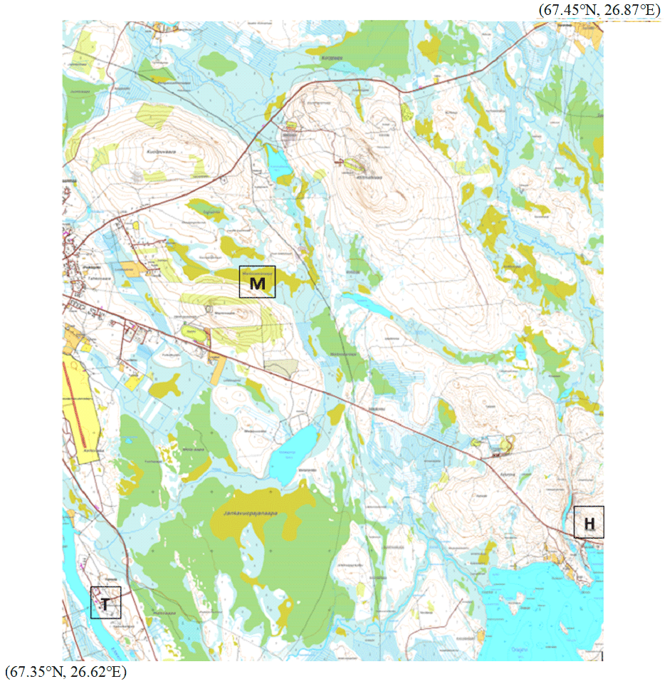
Figure 1Test area in Sodankylä in northern Finland. The premises of the Arctic Space Centre of FMI are situated in Tähtelä (T). The operational albedo measurements are located in the upper part of the rectangle surrounding T and the NorSEN mast at the lower part. The aapa mire test site Mantovaaranaapa is marked with M and the forest clearing site Hirviäkuru with H. The corner coordinates of the area given in the WGS84 system. CC BY 4.0 National Land Survey of Finland (04/2020).
2.2 Grain size and density profiles of snowpack
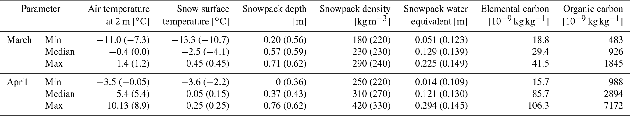
Measurements of snow depth, total density, water equivalent (SWE), humidity profile, temperature profile, grain size profile, surface roughness and surface impurity content were carried out at snow pits located in Sodankylä in an area with corner coordinates (67.36∘ N, 26.63∘ E; 67.45∘ N, 26.86∘ E) in March and April 2009 and in March 2010 (Manninen and Roujean, 2014). In addition, crystal size photos of the snow layers, surface roughness photos and photos of the top surface impurities were taken. In this study we concentrate on the values measured in 2009. The air temperature in March was mostly below 0 ∘C, whereas in April it was above 0 ∘C almost all the time (Table 1). Hence, April represents the melting season and March is still midwinter. This is also clear from the increase in median density of the snowpack and the decrease in median snow water equivalent value from March to April. About 40 snow pit measurement points were located in a larger area (67.42∘ N, 26.04∘ E; 67.85∘ N, 26.91∘ E), where the maximum measured snow depth was 0.92 m in March and 0.76 m in April. The total density varied in the range 180–320 kg m−3 in March and in the range 270–570 kg m−3 in April. The corresponding variation ranges for the snow water equivalent were 0.020–0.250 and 0.034–0.239 m, but in April there was plain water in several places in the snowpack. Hence, the area covered by the snow pit measurements represents the local variation of snow properties to a large extent.
Table 1The variation range and median values of the air temperature and snow surface temperature during the SNORTEX campaign in Sodankylä in 11–19 March and 20–27 April 2009. The corresponding variation of the snow density and snow water equivalent are given as well. The measurements were carried out during 09:00 and 17:00 h local time (Manninen and Roujean, 2014). The values in brackets are those measured at the reference site NorSEN mast (67.3621∘ N, 26.63445∘ E) in Tähtelä. The total number of individual measurements was altogether 118 (17) for the reference site. The elemental carbon and organic carbon concentrations measured near the NorSEN mast (67.364011∘ N, 26.635891∘ E) in March and April are shown as well (Meinander et al., 2020).
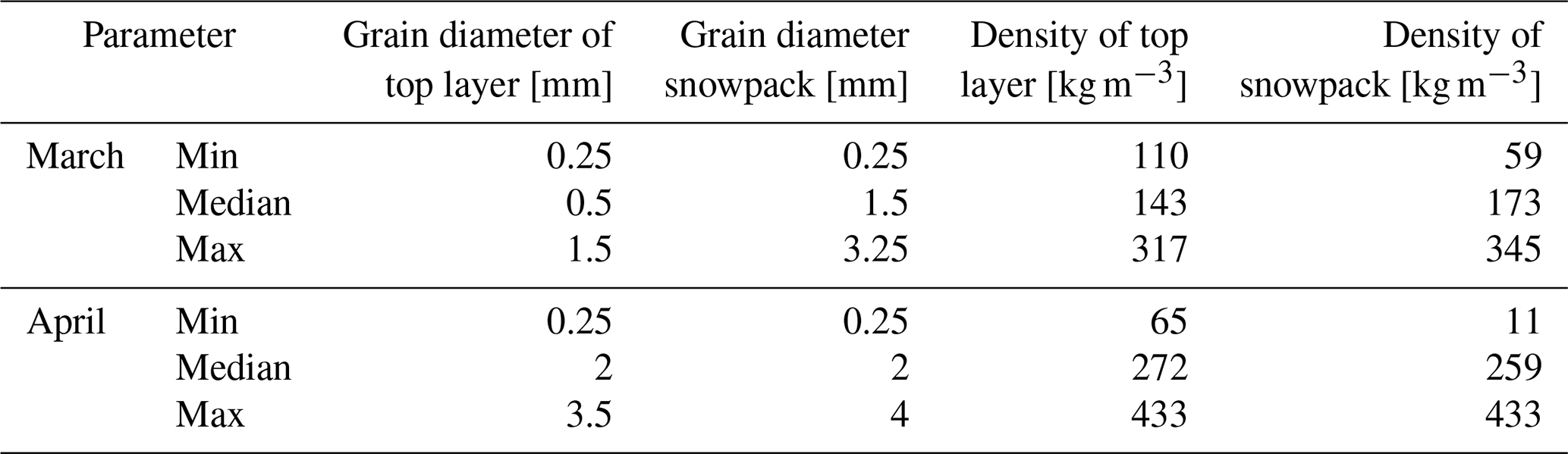
The traditional snow grain size (the largest dimension of the snow grains, Fierz et al., 2009) was visually estimated using graded plates, collecting the snow crystals from 10 cm thick snow layers from the bottom to the top of the snowpack. For each analysed sample of snow crystals, in addition to the typical value of the largest grain dimension also its minimum and maximum value were provided. The measured snow grain sizes differ from the optically equivalent snow grain size (Mätzler, 1997; Neshyba et al., 2003). To partly compensate for this, the minima of the largest grain diameter were applied in the radiative transfer calculations as the effective diameter. Although this causes some uncertainty in the interpretation of the computed absolute albedo values (particularly for the cases of fresh snow), it has much less impact on the derived effect of small-scale surface roughness on snow albedo. The density profile of the snowpack was measured for the same layer structure using the snow fork (Toikka, 1992). The variation range of the grain size and density is shown for the surface layer and for the whole snowpack in Table 2.
Table 2The variation range and median values of snow grain size (defined as the maximum diameter of the smallest snow grain in each sample) and density of the topmost layer and the snowpack during the SNORTEX campaign in Sodankylä in 11–19 March and 20–27 April 2009.
2.3 Surface roughness from plate measurements
The surface roughness up to 1 m scale was measured in March and April 2009 and in March 2010 by taking photos of a graded plate placed perpendicularly in the snowpack (Fig. 2). The snow surface profiles were automatically calculated from the photos using an image processing technique and the scale at the edge of the plate (Manninen et al., 2012). Control points at the scales were used both for the removal of the barrel distortion of the camera optics and transformation of the pixel coordinates to millimetres with photogrammetric methods. The plate surface roughness measurements were carried out at the same sites as the snow pit measurements (Sect. 2.2). At each site, profiles were measured in two perpendicular directions with a 1 m interval along 50 to 100 m distance.
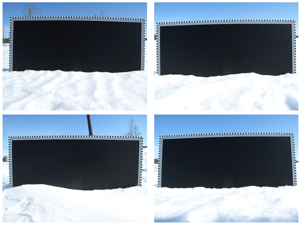
Figure 2Examples of surface roughness of snow at Mantovaaranaapa on 22 April 2009. The black background of the plate is 1 m wide.
The surface profiles were used to derive the root mean square (rms) height and correlation and their distance dependence (Keller et al., 1987; Church, 1988). Details of the multiscale roughness theory are described by Manninen (2003), and its application to the snow profiles is presented by Anttila et al. (2014). The snow surface roughness is close to a Brownian fractal surface (Anttila et al., 2014) so that the logarithm of the rms height σ depends linearly on the logarithm of the length x of the analysed profile used for its calculation, and the corresponding correlation length L is linearly related to x:
where a, b, k0 and k are constants, and k0=0 for an ideal Brownian surface (Russ, 1994). For each profile the values of the constants were calculated by linear regression using varying sliding window sizes, i.e. varying values of x (Anttila et al., 2014).
In addition, the rms slope angles β, i.e. arcus tangent of the slopes , were calculated for the measured spatial resolution, which was on average 0.26 mm. The vertical precision was about 0.1 mm and the horizontal precision 0.04 mm (Manninen et al., 2012).
2.4 Surface roughness from laser scanning
In addition to the plate measurements, laser scanning data for snow roughness were utilized. The laser scanning data used in this study have been acquired using the FGI ROAMER system (Kukko et al., 2007). The system, including a FARO Photon 120 laser scanner, a NovAtel SPAN GPS–IMU system, and data synchronizing and recording devices, was mounted on a sledge, which was towed by a snowmobile. The data acquisition covers a 2.5 km zone at each side of an official snowmobile track (see Kukko et al., 2013, for examples of profiles, the snowmobile track and other details). The landscape covered sparse pine forests and open bogs. The absolute precision of these measurements was analysed by Kaasalainen et al. (2011) to be better than 5 cm, while the relative accuracy (which is more relevant for observing the snow roughness) was found to be 0.7–2 mm for a static system and better than 10 mm when the snowmobile was moving. The best repeatability was achieved at ranges closer to the scanning system, i.e. below 5 m. The data quality and precision were controlled using control points measured with a virtual reference station (VRS) precision GPS (Leica SR530 receiver + AT502 antenna).
The laser profiles (about 16 profiles per 1 m at 3 m s−1 snowmobile velocity) measured on 18 March 2010 were used to analyse the variation of the slope angles in a larger area than was possible using the plate profiles. The profiles covered an area that was 2.4 km long, and the width extended into 3.2 m at both sides of the snowmobile. The slope angles for successive points were determined for each scan of the whole data set. The slope angles were then binned according to the horizontal distance between the successive points, with a bin width of 10−5 m. Then the root-mean-square value of the slope angles was determined for each horizontal distance bin, and a regression function for the dependence of slope angles on distance between successive points was derived.
2.5 Snow impurity content
The snow impurity was measured by filtering a melted sample of snow. The quartz filters were analysed using the NIOSH 5040 protocol. The increase in the median amount of impurities from March to April is obvious from Table 1 (Meinander et al., 2013; Meinander et al., 2014; Meinander et al., 2020). The detection limit of the thermal–optical OCEC method is 0.2 µgC, and the uncertainty of the OCEC is estimated to be ± 0.2 µgC (±5 % relative error for higher loaded samples). The relative portion (±5 %) is composed of the instrument variation and slight variations due to sample deposit inhomogeneity and sample handling, as we recently discussed more in detail in Meinander et al. (2020).
2.6 Surface albedo
The surface albedo was operationally measured at Sodankylä (67.36664∘ N, 26.628253∘ E downward; 67.36695∘ N, 26.62973∘ E reflected) with a 1 min interval using Kipp & Zonen CM11 pyranometers. The site is surrounded by trees and houses, so that shadowing takes place in certain azimuth directions, when the solar elevation is very low. Hence, the measured white-sky albedo values are considered more reliable than the blue-sky values. The least shadowed azimuth direction in early March corresponded to the solar zenith angle value of 73∘ in the afternoon. Thus, the blue-sky albedo values used in the analysis were all taken from the afternoon, when the solar zenith angle equalled 73∘. This means that the azimuth direction used increased a bit during the spring, but it did not cause any additional shadowing problem. Yet, the clear-sky albedo of 12 March was replaced with the diffuse albedo dominating that day, because the clear-sky albedo value of a narrow time window seemed unrealistically small. Albedo values measured at the NorSEN mast on 21 April 2009 using a portable Kipp & Zonen CM14 albedometer were used to calibrate the operationally measured albedo data in order to correct for the slight difference in location of the upward- and downward-looking pyranometer used for operational measurements.
The portable albedometer was used in April 2009 to measure the snow surface albedo in the same areas where the snow pits were made (Sect. 2.2). The instrument was installed on a short boom affixed on a lightweight camera tripod for easy transport. The tripod legs affect somewhat the reflected radiation measurements, and therefore a first-order correction, multiplication by 1.055, was applied. It was based on estimation of the solid angle blocked by the tripod legs from a fisheye lens photograph with a camera mounted onto the albedometer position on the tripod, assuming a constant albedo of 0.1 for the dark carbon fibre legs. The albedometer was calibrated against a reference pyranometer at FMI in Helsinki prior to each campaign. The albedometer was carefully levelled on the tripod before measurements at each location and the stability of levelling monitored regularly, as melting snow may become unstable during the day.
2.7 Spectral reflectance
The spectral reflectance of snow was measured using the ASD FieldSpec Pro JR spectrometer on several days, specifically in the perfectly overcast conditions on 13 March and on the perfectly clear-sky day of 22 April, during the campaign in 2009. The irradiance spectra were measured as well. Every spectrum is an average of 30 individual spectra. The spectrometer was calibrated by the manufacturer prior to the campaigns. The instrument was powered on at least 15–20 min before each measurement to ensure an even operating temperature. A Spectralon panel (0.125 × 0.125 m2) was used as white reference for the reflectance measurements. The Spectralon panel was housed in a container with two orthogonal spirit levels, placed on the snow and levelled. Narrow-view foreoptics were used to ensure that the field-of-view (FOV) fits fully onto the Spectralon panel. This was further visually confirmed by looking through the foreoptic before inserting the fibre optic cable. The white reference was measured, and then the tripod was carefully rotated so that the foreoptic pointed into pristine snow. Tripod leg shadowing on the measured area was carefully avoided for both white reference and snow measurements. Most measurements took place from a height of 0.5–0.6 m with an 8∘ foreoptic. The spectrometer was optimized before each measurement.
2.8 BRF
The bidirectional reflectance factor BRF of snow was measured using the Finnish Geodetic Institute's Field Goniospectrometer (FIGIFIGO; Peltoniemi et al., 2005, 2015, 2014). FIGIFIGO consists of a motorized arm of length of 2 m, moving the optics head ±90∘ around nadir, and an ASD Field Spec PRO FR spectrometer recording the spectrum in the range of 350–2400 nm. The azimuth is turned manually, and all angles and coordinates are recorded automatically, based on inclination, direction and position sensors. The footprint is around 0.10 m in diameter. FIGIFIGO gives spectrally resolved BRF data, relative to Spectralon reference standard (of the size of 0.25 × 0.25 m2, connected to a screw-adjustable mount and levelled with a bubble level), from which also spectral albedo can be evaluated by fitting a polynomial function and integrating over the hemisphere. However, as the system is not absolutely calibrated in the field setup, external solar spectrum is needed for deriving real broadband albedos and BRF. In the results shown, a mean solar spectrum is used that may differ several percent from the real-time one.
In Mantovaaranaapa, three sets of rough snow were measured, as well as one set of smoother snow formed by a thin layer of windblown grains. Another set of thin and rough snow was measured in Korppiaapa, but this was not used in the present study. The sunlight measurements were complemented by set of artificial light measurements of smoother snow near the NorSEN mast.
3.1 Smooth snowpack albedo modelling
The TARTES model (available at: https://snowtartes.pythonanywhere.com/, last access: 8 March 2020) was used to estimate the snowpack white-sky and black-sky albedo values (Warren, 1984; Warren and Brandt, 2008; Kokhanovsky and Zege, 2004; Baldridge et al., 2009; Libois et al., 2013, 2014; Picard et al., 2016). It is a fast and easy-to-use optical radiative transfer model and represents the snowpack as a stack of horizontal homogeneous layers. Each layer is characterized by the snow grain size, snow density, impurities amount and type, and two parameters for the geometric grain shape: the asymmetry factor and the absorption enhancement parameter. The albedo of the bottom interface can be prescribed (here 0.13), although the bottom interface only markedly impacts thin snowpacks (< 5 cm depth). The model is based on the Kokhanovsky and Zege (2004) formalism. The required input values for the model (density and grain size profile) were provided by the snow pit measurements of the SNORTEX campaign (Manninen and Roujean, 2014; Sect. 2.2). The amount of impurities was temporally interpolated from the values of measured days. The black-sky albedo values of the bulk snowpack were derived by weighting the spectral albedo with the standard top-of-atmosphere (TOA) spectrum ASTMG173. The white-sky albedo values of the bulk snowpack were derived by weighting the spectral albedo with measured diffuse irradiance spectra of the cloudy day 13 March 2009.
The black-sky albedo values were calculated for three local incidence angle values of each plate surface roughness profile: the mean, the mean minus 1 standard deviation, and the mean plus 1 standard deviation of the individual local incidence angle values determined for each slope of the surface roughness profiles. The nominal incidence angle was set to the solar zenith angle value at the time of the measurements of the plate surface roughness profiles and the density and grain size values of the snowpack layers. The blue-sky albedo values were obtained from the black-sky and white-sky albedo values using the fraction of diffuse irradiance operationally measured at Tähtelä.
3.2 Rough snowpack albedo modelling
From the theoretical point of view there is a difference in scattering from a snowpack having an ideally planar surface and a rough surface, because the rough surface may have an incidence angle distribution that markedly differs from the Gaussian distribution of incidence angles produced by a random volume of spherical scatterers partly shading each other. In addition, the roughness may cause a markedly higher amount of multiple scattering, thus reducing the amount of radiation escaping the target.
Scattering from randomly rough continuous surfaces is related to the characteristic size of the surface roughness with respect to the wavelength used (Beckmann and Spizzicchino, 1963; Ulaby et al., 1982; Tsang et al., 1985; Fung, 1994). When the surface roughness of a randomly rough continuous surface is large compared to the wavelength of the electromagnetic wave, the scattering of the wave from the surface can be approximated by scattering from random facets (i.e. using the Kirchhoff approximation), whose slopes determine the scattering directions. As the shortwave illumination covers the wavelength range of about 300–2500 nm, all structures in the millimetre scale (or above) are large compared to the wavelength, so that a facet-based surface scattering calculation is reasonable. Each facet is taken to represent a volume of random scatterers, and the local incidence angle of the incoming radiation is the angle between the normal of the facet and the solar zenith angle (Fig. 3). The surface of a snowpack is not a continuous solid surface, but when the snowpack surface is rough, the incidence angle distributions of the scattering elements may deviate from that of a planar surface with randomly oriented scatterers. In addition, it is possible that a photon escaping one facet hits another facet. The snowpack scattering can then be thought to have elements both of bulk volume scattering and surface scattering. The following 2D analysis demonstrates this idea.
Multiple scattering between facets can be taken into account using the photon recollision probability theory (Knyazikhin et al., 1998; Panferov et al., 2001; Smolander and Stenberg, 2005; Rautiainen and Stenberg, 2005; Stenberg et al., 2008; Stenberg and Manninen, 2015; Stenberg et al., 2016). The formulation is shown in Appendix A separately for diffuse and direct irradiance. The essential equations are repeated here. Firstly, for the diffuse case, the white-sky albedo αw (Lucht et al., 2000, Schaepman-Strub et al., 2006) is related to the average number of facet-to-facet scattering events :
where αw0 is the white-sky albedo of the bulk volume.
Second, for direct illumination, the black-sky albedo αb(θi) (Lucht et al., 2000, Schaepman-Strub et al., 2006) is approximately related to the αw0, and the average number < m(θi)> of facet-to-facet scattering events in direct illumination conditions by
where αb0(θi) is the black-sky albedo of the bulk part of the snowpack (i.e. the albedo without the surface roughness contribution). In this study the bulk albedo values αw0 are produced using the TARTES model (Sect. 3.1).

Figure 3Facet structure of a randomly rough surface of spherical scatterers. The arrows indicate an example of a possible ray path involving facet-to-facet scattering.

Figure 4Surface characteristics calculated from the plate measurements in March and April. (a) The relative height distributions and (b) the distributions of the slope angles (in degrees) at the average measured spatial resolution of 0.26 mm.
The albedo α in mixed illumination conditions is typically estimated using the weighted mean approximation of the two extreme values αw and αb (Lucht et al., 2000; Schaepman-Strub et al., 2006; Román et al., 2010):
where f is the fraction of diffuse irradiance. According to Eqs. (3)–(5) the blue-sky albedo is then estimated from
Obviously, surface roughness decreases the white-sky albedo and typically also the black-sky and blue-sky albedo. Only when is larger than , surface roughness can increase the black-sky albedo of bright targets. The effect of surface roughness is non-negligible even when the roughness is not large. On the other hand, the larger the roughness is (i.e. the larger and are), the larger the effect is for darker targets. Hence, for snow the effect is larger in the near-infrared than in the visible wavelengths and in midwinter roughness alters the broadband albedo only slightly, whereas during the melting season, when the snow is darker, the effect of the roughness may be much larger. Thus, the effect of surface roughness would be larger for old snow than for new snow, which may explain part of the quick darkening of snow during the melting season.
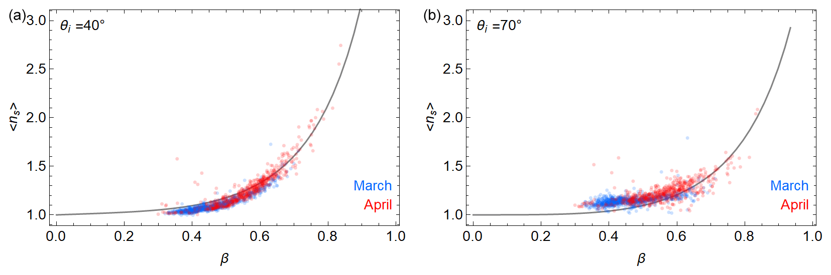
Figure 5The average number of reflections of an individual ray hitting the surface as a function of the rms slope angle β (in radians) for two incident solar zenith angle values θi for the snow profiles measured in the SNORTEX campaign (Manninen and Roujean, 2014; Anttila et al., 2014) in March and April 2009.
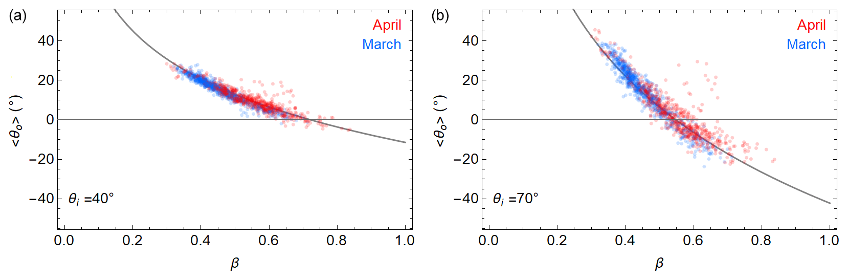
Figure 6The average zenith angle θo of the reflected escaping individual ray as a function of the rms slope angle β (in radians) for two irradiance solar zenith angle values θi for the snow profiles measured in the SNORTEX campaign (Manninen and Roujean, 2014; Anttila et al., 2014) in March and April 2009. The sign of the zenith angle is positive for forward reflection and negative for backward reflection.
3.3 Ray tracing analysis of surface roughness
Scattering from the snow profiles measured using the plate was analysed by a ray tracing method using 1000 equally spaced rays per profile per direction. The number of hits ns on the surface (unity for single reflection and larger for multiple surface scattering) and the direction of the escaping reflected ray were calculated as a function of the zenith angle of the incoming ray with an interval of 2∘ from 0 to 80∘. Scattering from the surfaces was calculated by assuming mirror reflection from smooth facets of continuous material, which has often been also assumed in the computation of ice crystal single-scattering properties in the solar spectral region (Nousiainen and McFarquhar, 2004; Zhang et al., 2004). This approximation neglects the impact on scattering due to snow structures smaller than the measurement resolution (∼ 0.1 mm for plate measurements). For each angle the case was calculated separately for rays coming from the left and from the right, and the two results were unified to improve statistics. This choice was motivated by the known fact that, even when the snow is highly forward scattering, it is with respect to the direction of the incoming solar radiation, not the wind direction. Thus, the dominant scattering direction moves with the sun during the day. In some cases, the ray was trapped to infinite reflection from facet to facet. But these quite rare (< 1 %) cases were excluded from the statistical analysis. Since the surface roughness profiles produce only 2D information and scattering angles differ markedly in 2D and 3D, the calculated ray-tracing-based 2D BRFs were converted to 3D versions assuming that each facet has besides the measured vertical angle also an azimuth angle obeying a random uniform distribution between 0 and 180∘. In fact, calculations were made for the range 0–90∘, assuming the case to be symmetrical with respect to azimuth angle, like in constructing the FIGIFIGO-based BRFs. The 3D conversions make the peaks of the 2D scattering angle distributions slightly less distinct. No atmospheric contribution was included in either data set.
Late in spring the scattering from a snowpack often also contains a component that is something between volume and surface scattering, namely deep narrow pits generated by impurities that have sunk downwards in the snowpack due to melting caused by absorption of solar radiation. This kind of an effect is not easy to take into account either in volume scattering or surface scattering, because they do not affect the roughness or density in a random way. Their contribution to albedo is beyond the scope of this study.
4.1 Surface roughness and inputs for albedo modelling
To start with, we consider the snow surface roughness from the plate measurements. The rms slope angle calculated from the plate roughness measurements had an increasing trend from March to April (Fig. 4). The surface height distributions developed towards a more Gaussian distribution from March (R2=0.97) to April (R2=0.99). However, it should be noted that individual profiles could deviate markedly from Gaussianity, as evidenced by the ratio of skewness to standard deviation. The 90 % quantile of this ratio for individual profiles was 0.36 in March and 0.13 in April. The ratio was not negligible for the monthly average distributions either (0.17 in March and −0.04 in April). Furthermore, the autocorrelation functions were in most cases not Gaussian (Anttila et al., 2014). The most common (41 %) autocorrelation function (ACF) type was multiscale exponential, and 66 % of the profiles had multiscale ACF (Anttila et al., 2014).
The mean number of individual reflections ns per ray on the surface has an increasing trend during the melting season (Fig. 5). It correlates well (83) with the rms slope angle (β, in radians) of the profile. A good general fit to all measured plate profile data was
where θi is the solar zenith angle. The mean zenith angle θo to which the radiation escapes from the surface (when mirror reflection from the facet is assumed) is even more strongly correlated (R2=0.93) with β (Fig. 6):
All angles (β, θi, θo) are given in radians in the above equations, and ) for forward-scattering (backward scattering). Obviously, the probability for backward scattering increases with increasing incidence angle and increasing β. Since β increases with time, also the probability for stronger backscattering from the snow cover increases with time. Indeed, it is well known that older snow cover is less strongly forward scattering than new midwinter snow (Peltoniemi et al., 2010).
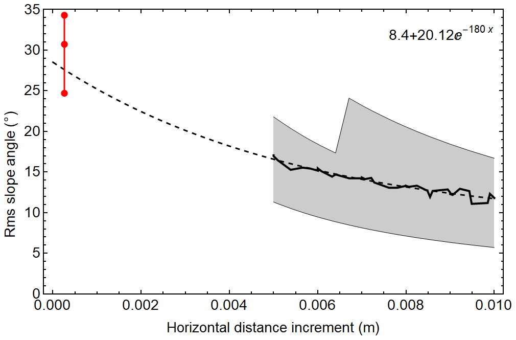
Figure 7Relationship between rms slope angle and the horizontal distance between the points used for its determination according to the laser scanning data of 18 March 2010. For comparison the mean value and variation range of the rms slope angle values derived from the 10 plate profiles for horizontal resolution 0.25 mm in the same area in the same day are shown in red. The dashed black curve is the regression to the 36 laser-scanning-based points (black polyline), and the grey shaded area covers the 80 % variation range of rms slope angle at the distance in question.
Unfortunately, the β values depend strongly on the scale of the measurements. The laser scanning data are well suited to demonstrate this, because the horizontal distance between successive data points increases from the beginning to the end of the scan line. On 18 March 2010 plate profile measurements and laser scanning were carried out in the same relatively flat wetland area of Mantovaaranaapa (67.4∘ N, 26.7∘ E). The laser scanning data covered a 2.4 km long and about 3.2 m wide area on each side of the snowmobile route. Altogether 10 plate profile measurements were taken directly after the scanning, at about 100–200 m intervals starting from the western edge of the scan route (Kukko et al., 2013). The average rms slope angle of the 10 plate profiles was 30.7∘ (β=0.54) with an 80 % variation range of 24.7– 34.3∘ (β=0.43–0.60). Consequently, ns would then vary in the range 1–1.5 (Fig. 5). The rms slope angles were calculated also from the laser scanning profiles as a function of horizontal increments, which were within the range 5–100 mm. The number of points per distance varied between 4 thousand and 2.2 million. Nonlinear regression to the 36 points in the range 5–100 mm produced an exponential curve that approaches the mean rms slope angle value obtained from the 10 plate profiles of the same area and Fig. 7. Shorter increments of the laser data could not be reliably used in the analysis.
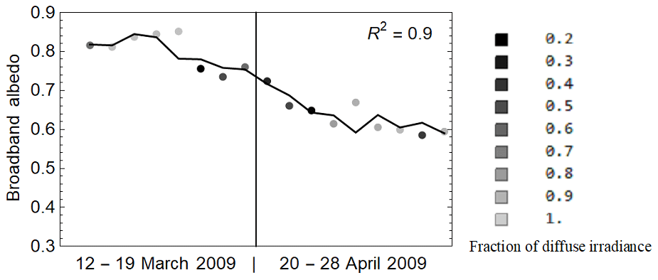
Figure 8The relationship between the albedo values corresponding to the solar zenith angle value of 73∘ measured operationally at Sodankylä and the regression (albedo = 0.84–0.29 b−0.008k0) based on measured surface roughness parameters b (Eq. 1) and k0 (Eq. 2) at the NorSEN mast in March and April 2009. The darkness of the markers is related to the fraction of diffuse irradiance.
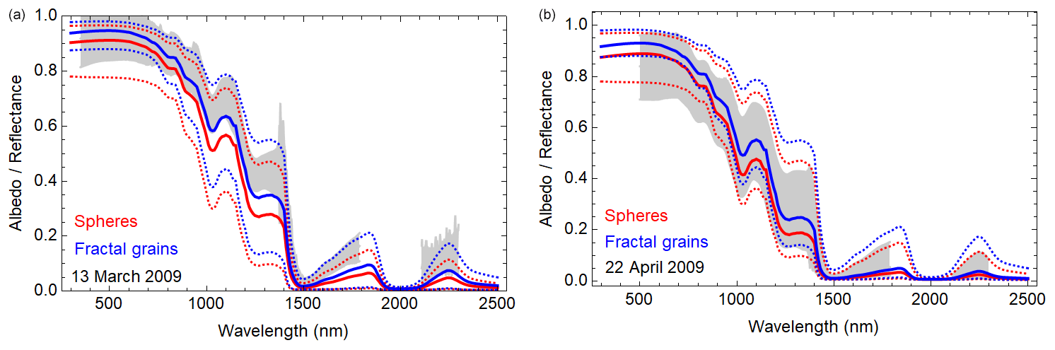
Figure 9Variation range (grey) of the individual snow reflectance spectra measured using the ASD spectrometer in Hirviäkuru (67.38∘ N, 26.85∘ E) on 13 March and in Mantovaaranaapa (67.4∘ N, 26.72∘ E) on 22 April. The albedo simulations using the TARTES model are shown for fractal grains (blue) and spheres (red). The solid lines indicate the mean value and the dotted lines the minimum and maximum curves of the day in question. The ASD measurements were carried out in the same area as the grain size and density measurements, but the impurity measurements were daily values measured at Tähtelä (67.37∘ N, 26.63∘ E).
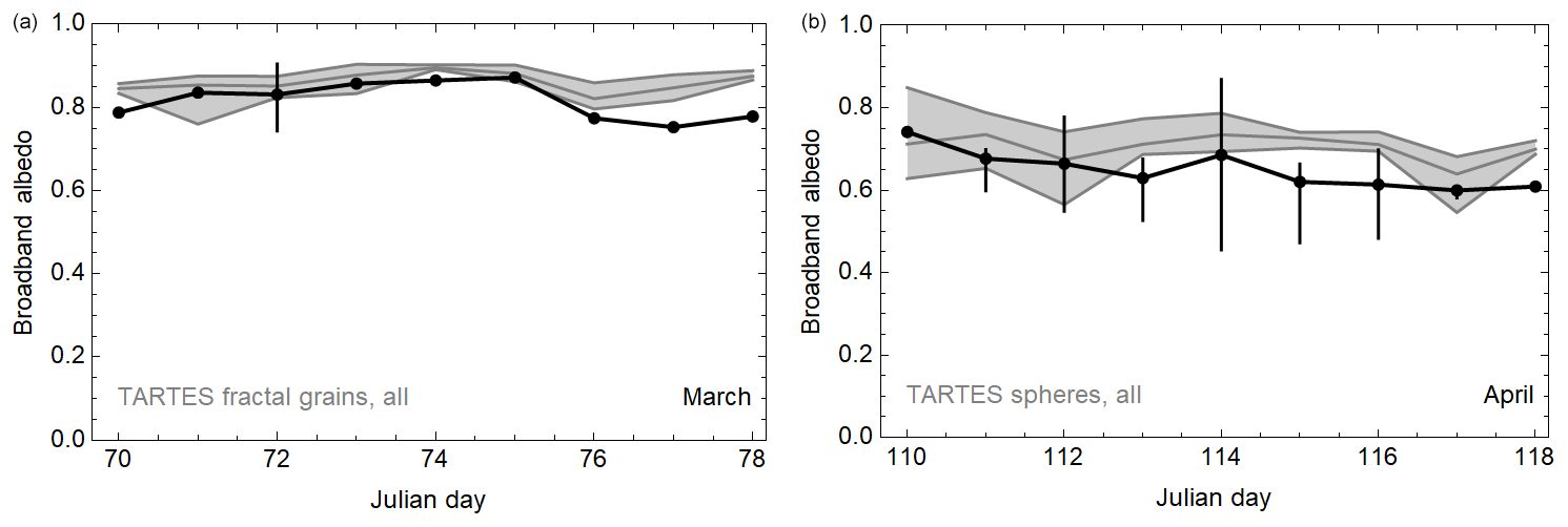
Figure 10Evolution of measured surface albedo in Tähtelä (67.37∘ N, 26.63∘ E) on 12–19 March and 20–28 April 2009. The corresponding variation range of simulated albedo values based on simultaneous grain size and density measurements and temporally interpolated impurity content in the same day are shown in grey. The minimum, mean and maximum values are indicated with darker grey curves. The vertical error bars marked for some of the measured albedo values are based on the variation range of the measured ASD-spectra-based broadband reflectance values during the same day in the larger test area in Sodankylä.
As the laser scanner covered a much larger area than the plate profiles, that data give an estimate of the rms slope angle variation in a larger area and are based on a larger number of individual slope angle values. For the laser data set, the median difference between the 90 % quantile curve of the slope angle values and the rms slope angle value curve was 6.1∘. The corresponding median difference for the 10 % quantile curve from the rms slope angle curve was −5.9∘. For the plate profiles, 90 % and 10 % quantile values of the rms slope angle differed from the mean rms slope angle value by 3.6 and −6.0∘. Thus, the larger area covered by the laser scanner shows a larger variation of the rms slope angle, as one could expect. Obviously, the laser scanner data can be extrapolated to estimate β at higher horizontal resolution than the measurements directly enable, but then β has to be analysed as a function of the horizontal distance increment (Fig. 7). However, the strong variation of β with spatial resolution suggests that using less scale-dependent surface roughness descriptors would be desirable, if they just can provide the information needed.
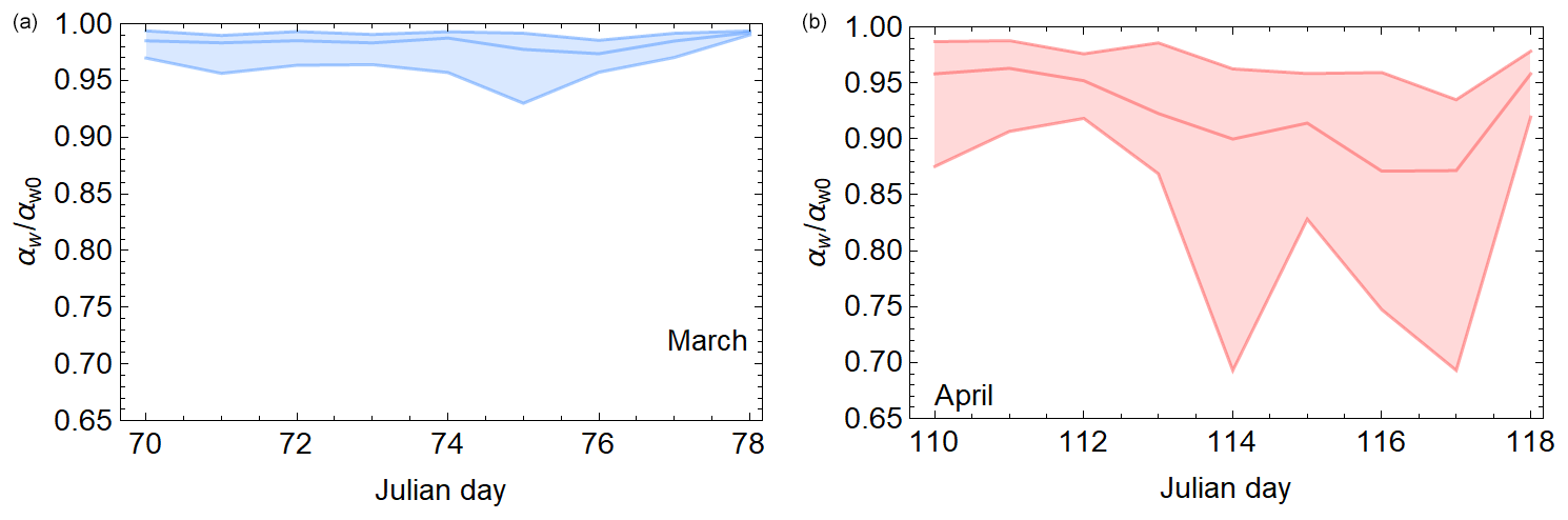
Figure 11Ratio of simulated total and bulk white-sky albedo values for all 1381 profiles and snow pit and impurity data in Sodankylä in 11–19 March and 20–28 April 2009. The daily mean, minimum and maximum values are indicated by the darker curve, and the variation range is shaded.

Figure 12Simulated albedo values at the NorSEN mast based on density, grain size and surface roughness measurements of snow in 12–19 March 2009 and in 20–28 April 2009 and temporally interpolated impurity content data. The mean values are shown separately for the TARTES model containing only the volume scattering contribution (grey curve) and the TARTES model combined with the surface scattering model of this study (blue or red). The daily variation range based on diverse profiles, grain size and density measured at the site and temporally interpolated impurity content are shown as the area shaded by light blue or light red colour. The darkness of the empirical points indicates the fraction of diffuse irradiance during the measurement.
The relationship between other surface roughness parameters (such as rms height σ and correlation length L) and β is in general not strong, even for a Gaussian surface height distribution (Beckmann and Spizzicchino, 1963). For the whole period (3 March–28 April 2009) the ratio of (determined for 0.60 m distance) correlated relatively well with β, with the R2 values being 0.70, 0.62 and 0.67 for the whole data range, March and April, respectively, but the best descriptor of β was found to be (Eq. 1), with its R2 values for the linear correlation being 0.78, 0.68 and 0.82 for the whole data range, March and April, respectively (data shown in the Supplement). β tends to increase with the progress of the melting season (0.002 rad per day). Likewise, its correlation with increases during the melting season. It was therefore examined whether the measured surface albedo correlates well with the measured surface roughness parameters. Using just the rms height (derived for a 0.60 m horizontal scale) as an explanatory variable of the albedo, the coefficient of determination was R2=0.81 (data shown in Supplement). The relationship between the albedo and surface roughness parameters that are scale-independent in a large range (Manninen, 2003) was then evaluated. Indeed, a simple linear regression for the data of March and April 2009 produced a coefficient of determination value as high as R2=0.90, when the parameters b and k0 (see Eqs. 1 and 2) were used as explanatory variables (Fig. 8). While correlation is not a proof of causality, this result supports the view that surface roughness affects the albedo.
4.2 Snow albedo spectra: measured vs. modelled
Two examples of snow nadir reflectance spectra measured with the ASD spectroradiometer are shown in Fig. 9. On 13 March, the sky was completely overcast, whereas on 22 April it was perfectly clear. For comparison, corresponding albedo spectra modelled using TARTES are shown. The ASD reflectance spectra were scaled so that the derived broadband reflectance value matched the calibrated operationally measured broadband albedo value. The scaling factor was 0.994 for the diffuse case of 13 March and 0.937 for the clear-sky case of 22 April. No BRF was available for the clear-sky case for the location of ASD, but for old rough snow in the area it was relatively flat (see Sect. 4.5), so that the comparison of the spectral reflectance and albedo values seems reasonable enough to enable the choice of the grain shape to be used in the TARTES model calculations. The spectra modelled with TARTES accounted for the empirical grain size and density values, as well as for black carbon but not for organic carbon (Table 1), which included needles and various tree trash deposited on snow. In March, the impurity content in surface snow was very low, while in April it was roughly 3 times higher (Table 1). In March a better fit is obtained using fractal grains, the result of which is also supported by photos taken of snow grains and the fact that the snow was fresh. In April the modelled albedo favoured the use of spherical grains rather than fractals in the calculations. The photos taken about the snow grains also supported the use of spherical grains in April. Thus, the TARTES results seem to represent the snowpack in March well, but in April when the melting has been going on for a longer time the modelled albedo values are higher than the empirical reflectance values both in the visible and near-infrared wavelengths (less than ∼ 1 µm), which dominate the value of the broadband albedo of snow. The grain size estimation uncertainty was not significant in April, because the grains were already very rounded, but in March the definition and estimation of the grain size was challenging. However, even if the actual grain size for fractal grains was as much as 1 mm larger than estimated, this would not in all cases provide the measured albedo value using the TARTES model without contribution of surface roughness. As the median grain size of the top layer was in March 0.5 mm and the corresponding maximum value was 1. 5 mm (Table 2), it is in practice highly improbable to make an error of 1 mm or more using a graded plate with 1 mm scale.
4.3 Broadband albedo: measured vs. modelled
The evolution of the operationally measured broadband albedo in Tähtelä is shown for the periods 12–19 March and 21–28 April in Fig. 10 together with the corresponding albedo values simulated using the TARTES model assuming a flat surface and the grain size and density measurements of the day in the Sodankylä area. Following the justifications outlined above and on the basis of photos taken in every test site, fractal grain shapes were used in March and spheres in April. The simulated values tend to exceed the measured ones, especially in April. In March the grain size estimation was difficult, because of the small dimensions of the very complex grain shapes. Hence, some but not all of the difference between the measured and modelled results may be explained by that. On the contrary, in April the grains were already very large and rounded, so that the difference between the modelled and measured values should not come from grain size uncertainty. Besides, the variation range of simulated albedo values is rather small compared to that of the empirical broadband reflectance values. However, it will be demonstrated next that taking into account the surface roughness decreases the difference between simulated and empirical albedo estimates.
The albedo model taking into account both volume and surface scattering (Eqs. 3–5) was applied so that αw0 was the value provided by the TARTES model based on the measured density and grain size profile and impurity content. The values for n and m were derived from the empirical values of ns. Namely, for the local solar zenith (θil) angle range derived using the ray tracing method. And n is the weighted mean of ns−1, where the weights are cos(θil)⋅sin(θil). The results are shown in Figs. 11 and 12.
First, the ratio of the total white-sky albedo and the bulk white-sky albedo provided by the TARTES model is considered in Fig. 11. In March, this ratio varies mainly between 0.97 and 0.99, indicating that small-scale surface roughness decreases the snow albedo typically by 1 %–3 %. With the progress of snowmelt, the effect of surface roughness increases markedly. On 26–27 April (Julian days 116–117), the median of falls below 0.9, indicating an over 10 % decrease in snow albedo. The relative difference between the total and bulk albedo values is about the same for the black-sky case as for the white-sky case, but the solar zenith angle naturally slightly complicates that relationship (see Eqs. 3 and 4). The larger variation of the values in the latter part of April (after Julian day 112) is related to vigorous melting of the snowpack, since then the measured temperatures were about 0 ∘C throughout the snowpack (Manninen and Roujean, 2014).
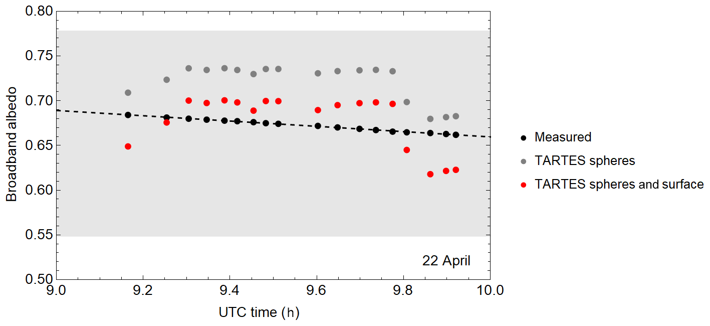
Figure 13Measured and modelled blue-sky albedo values at Mantovaaranaapa on 22 April 2009. Each modelled point is an average corresponding to three individual plate profiles taken from the same surface. The empirical albedo values are likewise averages of the three individual points recorded using the Kipp & Zonen albedometer CM14 at the time of taking the profile photos. The shaded area shows the variation range of the broadband reflectance values measured using the ASD spectrometer.
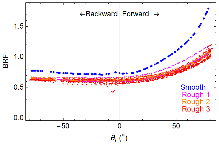
Figure 14Measured principal plane BRFs in Mantovaaranaapa on 22 April 2009 of one smooth snow and three rough snow cases, with a few individual profiles each.
The modelled albedo values are further compared to observations in Fig. 12. The variation range of the simulations shown with the background shading is based on the variation of the grain size, density and local incidence angle of the measured profiles. Overall, the inclusion of surface roughness significantly improves the agreement of modelled albedos with the observed ones. A notable overestimation remains, however, on Julian days 77–78 and will be discussed in Sect. 5. All in all, the model is robust enough to be reasonably applied to empirical data of grain size, density and surface roughness.
Obviously, taking into account the surface roughness contribution improves the match of empirical and modelled results, but still it is very clear that the grain size, grain shape and SWE (or density) are dominant parameters, because the amount of volume scattering also affects directly the amount of surface scattering. The variation range of the modelled albedo is much larger for clear-sky cases than diffuse cases, which is understandable as some of the variation in clear-sky cases comes from the solar zenith angle variation during the day.
4.4 Albedo during snow metamorphosis on 22 April
The modelled albedo results were compared with the Kipp & Zonen CM14 albedometer measurements carried out in Mantovaaranaapa on 22 April 2009, which was a perfectly clear day (Fig. 13). One snow pit was measured during 09:00–10:00 UTC at 67.40735∘ N, 26.72357∘ E. The albedometer was positioned in its vicinity and it recorded the metamorphosis process shown by the linear (R2=0.998) decrease in the albedo with time. Surface roughness of 54 individual profiles was retrieved with the plate method with typically 10 m incremental distance in perpendicular directions covering an area of about 100 m × 100 m (Fig. 2). Each position of the plate was photographed three times, so that 18 separate profiles were characterized. Hence, the modelled albedo results were averaged to get one value per surface sample. The light grey band in Fig. 13 shows the variation range of the broadband-converted reflectance spectra measured with the ASD spectrometer in the same area at the same time. Obviously, the modelled profile albedos fit in that range. The mean of the empirical albedo values is 0.67 and the modelled mean values are 0.72 and 0.68 for volume scattering only and for both volume and surface scattering, respectively. Taking into account the snow surface roughness thus improved the average modelled albedo estimate.
4.5 BRF
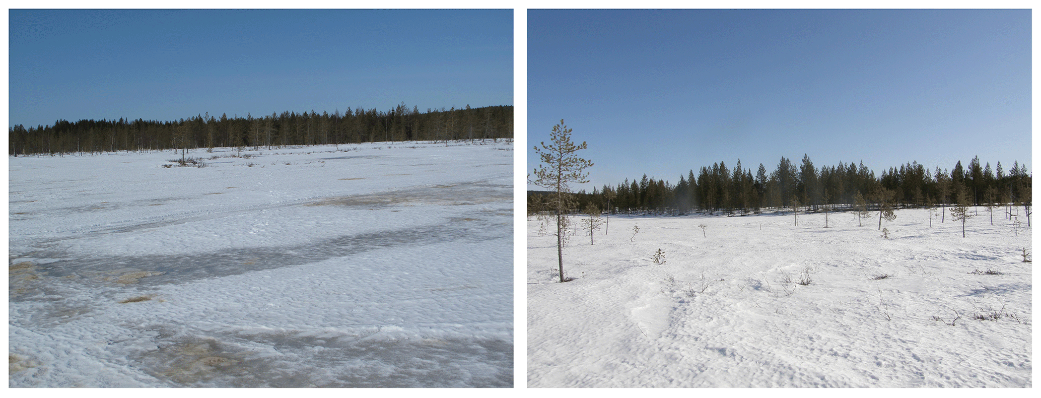
Since the contribution of surface roughness to the total albedo is markedly smaller than the contribution of the bulk volume scattering (i.e. scattering of a snowpack with an ideal plane surface), it is clear that the volume scattering dominates also the BRF. However, the contribution of surface roughness is not negligible, and the BRF of the surface scattering component may differ markedly from the bulk volume component, resulting in a complex total BRF. The ray-tracing-based surface BRFs (without any volume scattering contribution) were compared with empirical BRFs measured using FIGIFIGO (Fig. 14) in Mantovaaranaapa on 22 April 2009. The area is an aapa mire, which late in spring affects the snow properties markedly (Fig. 15). Sporadically the snow had melted and refrozen.
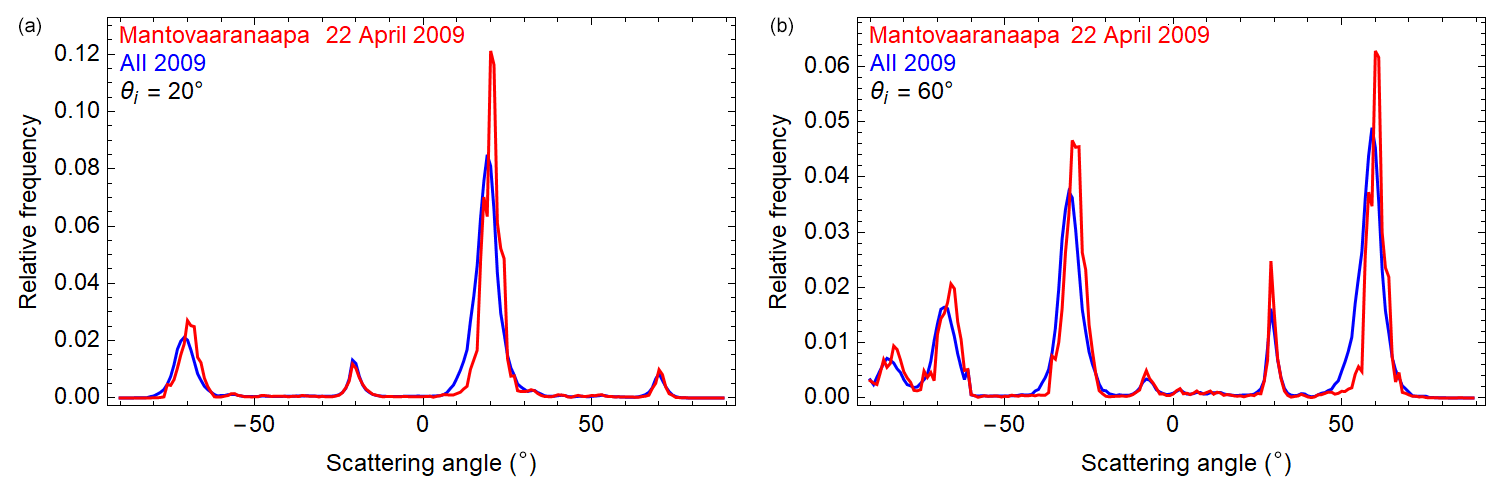
Figure 16Calculated average scattering angle distributions for surface scattering (i.e. zenith angles of reflected radiation, positive for forward directions and negative for backward directions) for profiles measured during the SNORTEX campaign in 2009 (blue) and in Mantovaaranaapa on 22 April 2009 (red) for incidence angle values 20 and 60∘.
Table 3The mean values and variation range of the ratio rfb of backward to forward scattering for diverse solar zenith angle values for all profiles measured in March and April 2009. These values represent the surface scattering contribution only.

The comparison of the ray-tracing- and surface-roughness-based BRFs with the empirical FIGIFIGO-based BRFs was made in the principal plane, since the azimuth information of the former ones was just a statistical assumption to convert the 2D principal plane BRF to the 3D principal plane BRF. The surface scattering BRFs are typically peaked to the direction θ of forward scattering matching mirror reflection of the surface plane of the snowpack. In addition, a backward peak in the direction θ-90∘ is also strong in most cases (Fig. 16). The balance between forward and backscattered intensity varies with incidence angle so that large incidence angles favour surface backscattering due to roughness (Fig. 17, Table 3). Although mere surface scattering would lead to dominantly backward scattering in Mantovaaranaapa due to the large incidence angle values (55–64∘ for FIGIFIGO BRFs), the empirical BRFs measured using FIGIFIGO dominated by the volume scattering are still dominantly forward scattering. The balance between forward and backward volume scattering is related to the grain shape (Peltoniemi et al., 2010). But indeed, the smoothest snow sample produced the least backscattering, and the ratio of the backward to the forward-scattered amount of radiation was 0.58, whereas the corresponding ratio was on average 0.73 for the rough BRFs. This result is quite in line with the general ray tracing analysis results that surface roughness increases the fraction scattered backwards (Table 3). Also, in a previous theoretical study of Gaussian surfaces it was shown that roughness affects the maximum direction of backward scattering (Jämsä et al., 1993). For the profiles measured in Mantovaaranaapa on 22 April the ratio of the backward- and forward-scattered radiation amounts in the incidence angle range of the FIGIFIGO measurements varied from 1.0 to 1.46. One has to take into account that the plate profiles register roughness in 1 m scale, whereas FIGIFIGO measures samples of 0.10 m diameter. Hence the largest spatial roughness may not necessarily show up as strongly in the FIGIFIGO results.

Figure 17Surface roughness parameter a as a function of surface roughness parameter b (Eq. 1) of the dominantly backscattering and dominantly forward scattering profiles for incidence angles 20, 40 and 60∘.

Figure 18Snow surface structure evolution during 16–18 March 2009. The centimetre scale is shown in the right images.
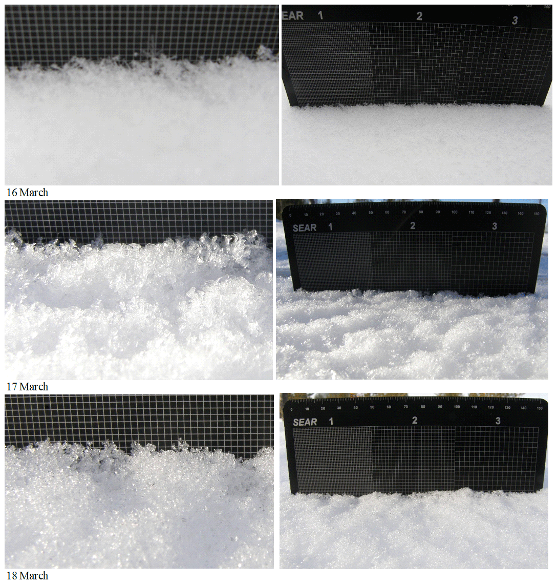
Figure 19Microscale snow surface structure evolution during 16–18 March 2009. In the left images the scale of the grid is 1 mm. In the right images the grids correspond to 1, 2 and 3 mm from left to right.
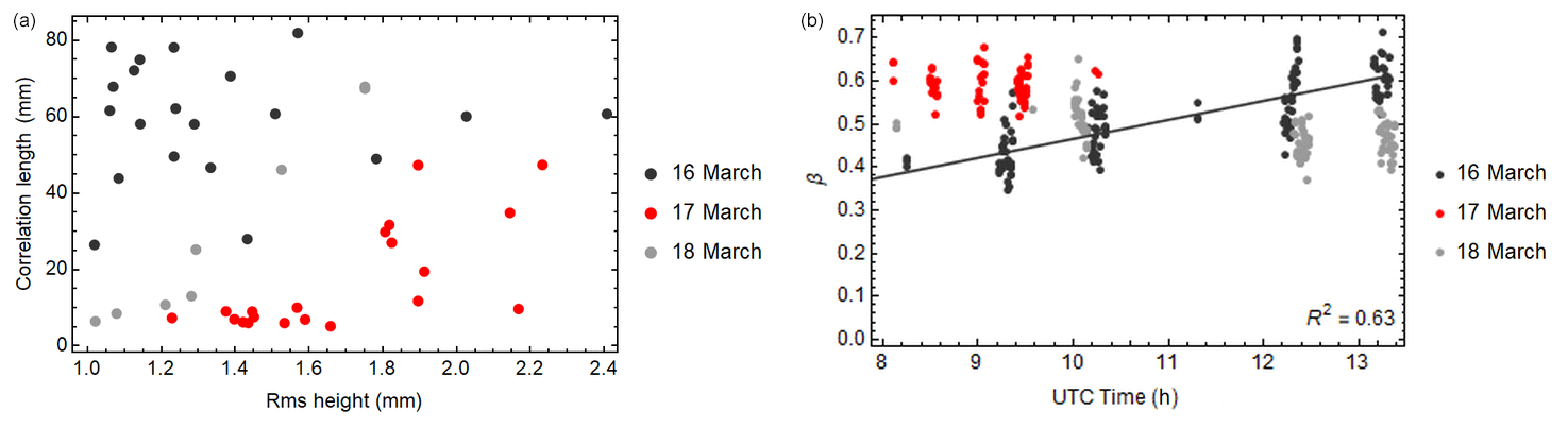
Figure 20(a) The snow surface rms height and correlation length measured with the plate method during 16–18 March 2009. The values correspond to the distance 0.6 m. (b) The rms slope angle β (in radians) of individual plate snow profiles during 16–18 March 2009. The linear regression for β vs. time is shown for 16 March, with the R2 value included.
In this study, the equations combining the volume scattering and surface scattering were derived using the photon recollision theory (Appendix A), because this theory could be extended to include the surface scattering effect. However, to describe properly the volume scattering of real snowpacks, it is essential to pay attention also to layer structure, grain shapes and various types of impurities, so that a more complex description is typically needed for realistic volume scattering estimation. In principle, the photon recollision theory could be extended to take the layer structure of the snowpack into account by just letting the photon recollision probability p to be a function of the depth, i.e. p=p(z), where z would be the distance from the bottom or top surface. However, that is beyond the scope of this study. Hence, the surface scattering part is developed so that in principle it can be combined with any volume scattering method. One just applies the estimates of αw0 and αb0 derived with the chosen volume scattering model in Eqs. (3)–(5). Hence, to obtain more realistic volume scattering estimates for the snowpack, we used the TARTES model for volume scattering in the simulations.
The findings that surface roughness in general decreases albedo and that the effect is larger for larger solar zenith angles are quite in line with the recent results obtained by applying a new rough-surface ray-tracing (RSRT) model to artificially generated surface roughness of snow (Larue et al., 2020). This study, however, extends these findings to smaller-scale roughness down to the sub-millimetre scale. The discussion about the effect of the varying local incidence angle on a rough surface and shadowing effects has been going on for decades, but until recently the emphasis has been on large-scale features (Warren et al., 1998; Kokhanovsky and Zege, 2004; Lhermitte et al., 2014). The essential advantage in studying the roughness from the theoretical point of view by generating artificial roughness with known dimensions and orientation is that one can then study the effect of each parameter involved separately (Larue et al., 2020). However, it is not trivial to generalize those results to natural snow, because the deterministic periodic structures may generate scattering features that will not be present for scattering from randomly rough surfaces. The advantage of the statistical approach presented in this study is that it does not make assumptions about the surface roughness characteristics but deals with the surfaces provided by nature. In addition, the derived formulas of the rough surface albedo are mathematically very simple and depend only on very few parameters, which makes their use very easy.
The ray tracing analysis of this study showed that the backward scattering increases with increasing surface roughness and increasing incidence angle of the illumination. However, that analysis concentrates only on surface scattering without any volume scattering contribution. Combining the surface and volume scattering contributions to BRF, perhaps using an adding procedure for radiative transfer, would be an interesting topic for future work.
Although the surface scattering model used here includes multiple scattering from the surface, it may be that a surface layer containing very deep cavities (in the scale of a few centimetres) would benefit from some special attention, like in the case of large-scale penitentes (Lhermitte et al., 2014). Namely, surface roughness measurements methods are usually designed for typical roughness of about the same variation range horizontally and vertically and not for extremely deep pits. To some extent the pit structure will be taken into account by the volume scattering models, since they affect the density of the surface layer of the snowpack. However, their very anisotropic (vertical) orientation is not well described by random scattering of a layer with reduced density. The pits act like illumination traps so that a larger part of illumination reaches lower layers of the snowpack before it is absorbed or scattered upwards. Therefore, the bulk albedo is smaller than for a completely random volume of the same density.
An example case is offered to illustrate this effect. Slight snow precipitation took place on 16 March so that a very fluffy surface structure of large dendritic snow crystals was formed on the snowpack (Figs. 18 and 19). The rms slope angle based on the plate method showed an increase with time from about 0.38 to about 0.63 with R2=0.68. The rms height and correlation length also manifested clear evolution during those days (Fig. 20). A related change is obvious also using the roughness parameters a and b (Anttila et al., 2014). Yet, the surface roughness measurements based on the plate method or laser scanning are not able to catch the deep pit structure of the surface, because of shadowing effects. Therefore, the simulated albedo is higher than the empirical one (Fig. 12, Julian days 76–78). However, even if the 2D-surface roughness were characterized properly, the surface scattering model based on a statistical approach of random scatterers would not be ideal for a case with a distinct periodic surface structure. For example, one could analyse separately the percentage of illumination that will be completely trapped by the deep cavities and reduce the simulated total albedo with that fraction.
The plate profile method has the advantage of high spatial resolution. Its main drawback is that it can be used only when the snow is relatively soft. It has been successfully used in Finnish Lapland (Anttila et al., 2014) and at Greenland Summit Station (Manninen et al., 2016), but Antarctic snow is typically so hard that it is not possible to immerse the plate in it. In addition, the icy and crusty snow surface of Finnish Lapland in 2018 and 2019 turned out to be too hard for the plate. For laser scanning, however, the hardness of the snowpack does not cause any problems. Indeed, laser scanning shows great potential for measuring snow surface roughness as it can cover large areas with high point precision accuracy. It is a particularly good method for measuring larger-scale roughness from 0.05–0.1 m upwards. The limiting factor in finer-scale roughness measurements is the data resolution and footprint size of the laser beam. So far, the scanners with the highest point density, accuracy and smallest spot size are meant for indoor use, but as the technology improves, smaller and smaller features become measurable also outdoors. In addition, the fractal nature of snow surfaces enables extrapolation of surface roughness from the centimetre scale to the millimetre scale (Kukko et al., 2013). Another benefit of using laser scanning for surface roughness measurements is that it leaves the surface intact. This enables repeatable measurements of the same surface, giving a means to study the evolution of surfaces in time. The backscattering intensity of the laser beam is typically stored for each point measured by laser, and in the most modern scanners also the range deviation is stored. These features have so far not been widely used, but they could potentially be used in the future for surface scattering property measurements and snow surface classifications.
Finally, considering satellite retrievals, it is expected that for an ideally flat surface the impact of roughness would be essentially the same at the satellite resolution as that in the scale of in situ measurements. However, the larger the satellite pixel is, the larger the spatial scale roughness that has to be taken into account is. The derived model is applicable to take into account roughness of all relevant scales, but the problem is how to estimate the average multiscale number of facet-to-facet scattering events. It is anticipated that due to the fractal nature of snow the small-scale estimate of the average number of facet-to-facet scattering events is a reasonable first-order estimate for the corresponding multiscale value, but a related detailed analysis is beyond the scope of this study.
A method was developed to model the effect of surface roughness on albedo besides the volume scattering. It can be combined with any volume scattering model. Applying measured surface roughness values to the model produced results closer to measured values than only volume scattering simulations made with the TARTES model. The surface roughness is described by the average number of surface scattering events per ray, which is currently estimated from the rms slope angle values of the measured surface roughness profiles. High empirical correlation (R2=0.9) of albedo with just two surface-roughness-related parameters supports the importance of surface roughness to albedo.
The albedo modelling results also taking into account the surface roughness indicate that it may decrease the albedo by about 1 %–3 % in midwinter and even more than 10 % during late melting season. The effect is largest for low solar zenith angle values and lower bulk snow albedo values. Hence, the effect is larger during early and late times of day everywhere, and it increases during the melting season especially at high latitudes, where the sun elevation is lower. Increasing surface roughness also favours more backward scattering.
A1 Scattering of diffuse radiation
The scattering of light in canopies has for several years successfully been described with spectral invariants and the so-called photon recollision theory, p theory (Knyazikhin et al., 1998; Panferov et al., 2001; Smolander and Stenberg, 2005; Rautiainen and Stenberg, 2005; Stenberg et al., 2008; Stenberg and Manninen, 2015; Stenberg et al., 2016). The central parameter, the photon recollision probability p, is spectrally invariant and depends on the amount of scattering surface in the volume. Canopies do not have distinct upper surfaces; hence the p theory is developed so far only for a scattering volume, but it has already been successfully combined with forest floor scattering also for snow-covered cases (Manninen and Stenberg, 2009). Here the p theory is applied to snowpack scattering taking into account that the snowpack has a distinct surface, which may be rough.
A simple way to take into account the surface roughness effect on scattering is to consider every facet of the snowpack as a separate volume of scatterers. When the irradiance i0=i0(λ) first arrives at the facet, it enters a volume scattering sequence, which can be described with the spectrally invariant photon recollision probability p of the bulk part of the snowpack and the single-scattering albedo of the snow grains ω=ω(λ) (Knyazikhin et al., 1998; Panferov et al., 2001). The radiation absorbed and radiation scattered by the volume of the facet a0 and s0, respectively, are (Smolander and Stenberg, 2005; Rautiainen and Stenberg, 2005; Stenberg and Manninen, 2015)
For simplicity the dependence of ω, i0, a0 and s0 on the wavelength λ is not shown explicitly in the equations. The radiation escaping the volume of the facet either escapes altogether or hits another facet and experiences another volume scattering sequence. The probability of the latter case is defined to be the surface photon recollision probability ps. Because the snow grains in the bulk part are completely surrounded by other snow grains while in the surface only close to half of the surrounding volume may contain snow grains, it is essential to assume that p and ps are not identical.
The radiation escaping the snowpack altogether without hitting another facet, r0, is
where q=q(λ) is the fraction of the volume scattering escaping upwards. Essentially it corresponds to Q defined by Stenberg et al. (2016, Eq. 24), but as it does not contain the fraction scattered upwards by the surface, it is not the total upward-scattered fraction of light. Hence q is used here instead of Q. Theoretically the values for q are in the range 0–1, being larger the thicker and denser the scattering layer is. The radiation hitting another facet is
The absorbed (a1) and scattered (s1) amounts of radiation by the second volume scattering sequence are
The amounts of radiation escaping (r1) and entering the following scattering sequence (i2) of another facet are
Formulas for the corresponding radiation components in the following facet-to-facet scattering round are
Further on, the components corresponding to the jth round are
The amounts absorbed and scattered by the surface and volume, considering up to n facet-to-facet scattering events, are then
Correspondingly, the upward-escaping radiation is
Note that when the number n of additional facet scattering sequences the photon has before it escapes altogether is zero and ps=0, there is no facet-to-facet scattering; i.e. the case is the normal volume scattering case. The total absorbed radiation and upward-escaping radiation of the snowpack are derived as infinite geometrical sums and are
The total white-sky (diffuse) albedo αw of the snowpack is then
The white-sky (diffuse) albedo of the bulk part of the snowpack (without facet-to-facet scattering) αw0 is
Hence, the total white-sky albedo is simply
Estimation of the parameter ps is not trivial, but when the distribution of n or its average value denoted by is known from measurements, then a reasonable estimate can be obtained from the total scattered energy s (Eq. A18) as follows. First, s is derived using the finite sum formulation of Eq. (A18) with a surface recollision probability of unity; i.e. ps set to 1. Second, s is derived using the probabilistic infinite sum formulation of Eq. (A18); i.e. n is set to infinity. These two estimates must equal. Taking into account Eq. (A23) and the normalized distribution f(n) of the values of n from zero to its maximum value nmax, the following relation is obtained:
which reduces to the following equation:
The value for ps can be solved from the above equation and is
In practice, the number of facet-to-facet scattering sequences n is often small, so that f(n) is dominated by values n=0 and n=1. When this is the case, the weighted mean of represented by the left part of Eq. (A26) can be approximated with a high precision with . This was indeed the case in the measured profiles. In March the normalized distribution was approximately and in April . Hence, the albedo estimation using instead of the distribution of n caused in March at most an underestimation of the total albedo by 0.004 and in April by 0.014. As reliable estimation of f(n) for single profiles is challenging, it is recommended to simply use the mean value . Then, the value of ps can be estimated from
The relationship between the total albedo and the bulk albedo is then
When the surface does not cause additional scattering, <n>=0 and the total albedo equals the bulk albedo. The larger the is, the smaller αw is.
For a single photon the number of facet-to-facet volume scattering rounds is naturally an integer number. For the ensemble of the photons, can be estimated to be
Combining Eqs. (A28) and (A30), it is possible to estimate q for values larger than 0, and it is
For <n>=1, q equals the bulk white-sky albedo, and for larger (smaller) values of it is slightly smaller (larger) for medium albedo values.
A2 Scattering of direct radiation
For the direct component of solar illumination one has to take into account that the irradiance depends on the solar zenith angle θi, i.e. , in addition to the wavelength. The photon recollision probability in the bulk snowpack will be denoted for the first scattering sequence p1=p1(θil) and for latter sequences p, assuming that the incidence angle dependence is lost after the first volume scattering sequence. Here the local incidence angle of the facet is denoted by θil. Then, the absorbed radiation of the volume will be (Stenberg and Manninen, 2015)
and the radiation scattered by the volume will be
When p1=p the above formulas reduce to Eqs. (A1) and (A2) as they should.
The first surface scattering sequence shall be treated separately, because the volume scattering depends on the incident solar zenith angle. The surface photon recollision probability is denoted by ps1=ps1(θil) for the first facet-to-facet scattering sequence and by psr for the latter facet-to-facet scattering sequences. One should notice that psr is not necessarily equal to ps of the diffuse case, although they certainly approach each other asymptotically. The reason for not taking them to be identical immediately is the typically small number of surface scattering events per ray of relatively smooth midwinter snow surfaces. The radiation escaping the facet altogether after just volume scattering, r0, is
where denotes the fraction of the scattered radiation escaping upwards from the snowpack during the first volume scattering sequence. The radiation hitting another facet is
The further scattering sequences are assumed to be independent of the solar zenith angle of the original incident radiation. The absorbed (a1) and scattered (s1) amounts of radiation by the second volume scattering sequence are then
The amounts of radiation escaping (r1) and entering the following scattering sequence (i2) are
Formulas for corresponding radiation components in the following round are
The components corresponding to the jth round are
The amounts absorbed and scattered by the surface and volume, considering up to m facet-to-facet scattering events, are then
Correspondingly, the upward-escaping radiation is
where m is the number of facet-to-facet scattering events. The total radiation escaping the snowpack upwards is derived again as an infinite geometrical sum
The total black-sky (direct) albedo αb of the snowpack is then
The black-sky (directional) albedo of the bulk snowpack αb0 is
Also taking into account Eq. (A23), the relationship between the total black-sky albedo and the bulk snowpack black-sky and white-sky albedo is
Estimating ps1 or psr (whether equal to ps or not) is not trivial, but like in the case of diffuse irradiance one can benefit from the measured average value of m denoted by by requiring that the total scattered energy (Eq. A49) is the same, whether it is calculated from the probabilistic infinite sum or a deterministic sum with surface recollision probability of unity, i.e.
Unfortunately, there are two variables, ps1 and psr, to solve but only one equation. Hence, the theory does not provide an exact solution for both ps1 and psr, but only psr remains explicitly in the equation of the black-sky albedo:
When the assumption that psr=ps is valid, the following formula is obtained for the black-sky albedo using Eq. (A28):
When , the black-sky albedo reduces to . Further on, when αb0=αw0, the total black-sky and white-sky albedo values are equal as well, if . The above approximation of the black-sky albedo is reasonable only when the assumption psr=ps is good. Hence, further studies are needed for proper estimation of psr and ps1.
The average number of facet-to -facet scattering rounds is estimated to be
When ps1→ps, q0→q and αb0 →αw0, approaches , as it should. It should be noted that the number of facet-to-facet scattering rounds in direct illumination () and in diffuse illumination () are not necessarily equal, with the difference being related to the difference of αb0 and αw0 and q and q0. The estimate for q0 can now be derived from Eq. (A58).
Some data of the SNORTEX campaign is directly listed in the report (Manninen and Roujean, 2014). The plate snow profile data and the ASD data are available upon request from Finnish Meteorological Institute. The FIGIFIGO measurements and the laser scanning data are available upon request from the Finnish Geospatial Research Institute, National Land Survey.
The supplement related to this article is available online at: https://doi.org/10.5194/tc-15-793-2021-supplement.
Albedo data were measured/retrieved and analyzed by TM and AR. Albedo modelling was carried out by TM, EJ, AR, JP, RP, J-LR, OH and PR. Plate surface roughness measurements and analysis were carried out by KA and TM. Laser scanning surface roughness measurements and analysis were carried out by SK, HK, AKu, KA and TM. FIGIFIGO BRF measurements and analysis were carried out by JP, JS and TH. Snow density and grain size profile measurements were carried out by PL, NS, LT and AKo. Snow impurity measurements and analysis were carried out by AKo, HS and OM. ASD snow reflectance spectra were measured and analyzed by AR, AKo, HS and TM. Ray tracing analysis was carried out by TM. Synthesis of analyses was carried out by TM, JP, PR and J-LR. Writing of the manuscript was carried out by everybody.
The authors declare that they have no conflict of interest.
The co-operation with the operational units of FMI in Helsinki and in Sodankylä and all SNORTEX campaign participants is gratefully acknowledged. The authors are indebted to Tuure Karjalainen for taking the plate-surface-roughness-related photos in the field in 2009. Panu Lahtinen, Niilo Siljamo and Laura Thölix took the other photos. The authors are also grateful to Markku Ahponen and Veikko Mylläri for the snow depth, density and SWE measurements of the remote points outside the intensive test area and to Markku Ahponen, Veikko Mylläri and Anita Sassali for participating in snow impurity sampling. The authors would like to thank Alexander Kokhanovsky, Ghislain Picard and an anonymous reviewer for beneficial comments.
The work was financially supported by the Academy of Finland in the projects SnowAPP (315497), OPTICA (295874), Reflectance of Boreal forests (120949), Scattering (260027), Arctic Absorbing Aerosols and Albedo of Snow (A4), (254195), and NABCEA (296302) and by EUMETSAT in the projects Satellite Application Facility on Climate Monitoring (CM SAF), Satellite Application Facility on Support to Operational Hydrology and Water Management (H SAF) and Satellite Application Facility on Land Surface Analysis (LSA).
This paper was edited by Marco Tedesco and reviewed by Alexander Kokhanovsky and one anonymous referee.
Anttila, K., Manninen, T., Karjalainen, T., Lahtinen, P., Riihelä, A., and Siljamo, N.: The temporal and spatial variability in submeter scale surface roughness of seasonal snow in Sodankylä Finnish Lapland in 2009–2010, J. Geophys. Res.-Atmos., 119, 9236–9252, https://doi.org/10.1002/2014JD021597, 2014.
Aoki, T., Kuchiki, K., Niwano, M., Kodama, Y., Hosaka, M., and Tanaka, T.: Physically based snow albedo model for calculating broadband albedos and the solar heating profile in snowpack for general circulation models, J. Geophys. Res., 116, D11114, https://doi.org/10.1029/2010JD015507, 2011.
Armstrong, R. L. and Brun, E. (Eds.): Snow and climate, Cambridge University Press, New York, USA, 2008.
Baldridge, A. M., Hook, S. J., Grove, C. I., and Rivera, G.: The ASTER Spectral Library Version 2.0, Remote Sens. Environ., 113, 711–715, https://doi.org/10.1016/j.rse.2008.11.007, 2009.
Beckmann, P. and Spizzicchino, A.: The Scattering of Electromagnetic Waves from Rough Surfaces, Pergamon Press, Oxford, UK, 497 pp., 1963.
Church, E. L.: Fractal surface finish, Appl. Optics, 27, 1518–1526, 1988.
Cook, J. M., Hodson, A. J., Gardner, A. S., Flanner, M., Tedstone, A. J., Williamson, C., Irvine-Fynn, T. D. L., Nilsson, J., Bryant, R., and Tranter, M.: Quantifying bioalbedo: a new physically based model and discussion of empirical methods for characterising biological influence on ice and snow albedo, The Cryosphere, 11, 2611–2632, https://doi.org/10.5194/tc-11-2611-2017, 2017.
Domine, F., Gallet, J.-C., Bock, J., and Morin, S.: Structure, specific surface area and thermal conductivity of the snowpack around Barrow, Alaska, J. Geophys. Res., 117, D00R14, https://doi.org/10.1029/2011JD016647, 2012.
Essery, R.: A factorial snowpack model (FSM 1.0), Geosci. Model Dev., 8, 3867–3876, https://doi.org/10.5194/gmd-8-3867-2015, 2015.
Fierz, C., Armstrong, R. L., Durand, Y., Etchevers, P., Greene, E., McClung, D. M., Nishimura, K., Satyawali, P. K., and Sokratov, S. A.: The International Classification for Seasonal Snow on the Ground, IHP-VII Technical Documents in Hydrology No. 83, IACS Contribution No. 1, UNESCO-IHP, Paris, 2009.
Flanner, M. G. and Zender, C. S.: Linking snowpack microphysics and albedo evolution, J. Geophys. Res., 111, D12208, https://doi.org/10.1029/2005JD006834, 2006.
Flanner, M. G., Shell, K. M., Barlage, M., Perovich, D. K., and Tschudi, M. A.: Radiative forcing and albedo feedback from the northern hemisphere cryosphere between 1979 and 2008, Nat. Geosci., 4, 151–155, https://doi.org/10.1038/ngeo1062, 2011.
Fung, A. K.: Microwave Scattering and Emission Models and Their Applications, Artech House, Boston, USA, 573 pp., 1994.
He, C., Takano, Y., and Liou, K.-N.: Close packing effects on clean and dirty snow albedo and associated climatic implications, Geophys. Res. Lett., 44, 3719–3727, https://doi.org/10.1002/2017GL072916, 2017.
Jämsä, S., Peltoniemi, J. I., and Lumme, K.: Thermal emission from a rough surface: ray optics approach, Astron. Astrophys., 271, 319–325, 1993.
Kaasalainen, S., Kaartinen, H., Kukko, A., Anttila, K., and Krooks, A.: Brief communication “Application of mobile laser scanning in snow cover profiling”, The Cryosphere, 5, 135–138, https://doi.org/10.5194/tc-5-135-2011, 2011.
Keller, J. M., Crownover, R. M., and Chen, R. Y.: Characteristics of natural scenes related to the fractal dimension, IEEE T. Pattern. Anal., 9, 621–627, 1987.
Knyazikhin, Y., Martonchik, J. V., Myneni, R. B., Diner, D. J., and Running, S. W.: Synergistic algorithm for estimating vegetation canopy leaf area index and fraction of absorbed photosynthetically active radiation from MODIS and MISR data, J. Geophys. Res., 103, 32257–32276, 1998.
Kokhanovsky, A. A.: Spectral reflectance of solar light from dirty snow: a simple theoretical model and its validation, The Cryosphere, 7, 1325–1331, https://doi.org/10.5194/tc-7-1325-2013, 2013.
Kokhanovsky, A. A. and Zege, E. P.: Scattering optics of snow, Appl. Optics, 43, 1589–1602, https://doi.org/10.1364/AO.43.001589, 2004.
Kokhanovsky, A. A., Lamare, M., Di Mauro, B., Picard, G., Arnaud, L., Dumont, M., Tuzet, F., Brockmann, C., and Box, J. E.: On the reflectance spectroscopy of snow, The Cryosphere, 12, 2371–2382, https://doi.org/10.5194/tc-12-2371-2018, 2018.
Komuro, Y. and Suzuki, T.: Relationship between the Concentration of Impurity and Albedo in Snow Surface, Atmospheric and Climate Sciences, 5, 426–432, https://doi.org/10.4236/acs.2015.54034, 2015.
Kukko, A., Andrei, C.-O., Salminen, V. M., Kaartinen, H., Chen, Y., Rönnholm, P., Hyyppä, H., Hyyppä, J., Chen, R., Haggrén, H., Kosonen, I., and Čapek, K.: Road Environment Mapping System of the Finnish Geodetic Institute – FGI Roamer, in: ISPRS Workshop on Laser Scanning 2007 and SilviLaser 2007, ISPRS, Espoo, Finland, 12–24 September 2007, 36, 241–247, 2007.
Kukko, A., Anttila, K., Manninen, T., Kaartinen, H., and Kaasalainen, S.: Snow surface roughness from mobile laser scanning data, Cold Reg. Sci. Technol., 96, 23–35, 2013.
Larue, F., Picard, G., Arnaud, L., Ollivier, I., Delcourt, C., Lamare, M., Tuzet, F., Revuelto, J., and Dumont, M.: Snow albedo sensitivity to macroscopic surface roughness using a new ray-tracing model, The Cryosphere, 14, 1651–1672, https://doi.org/10.5194/tc-14-1651-2020, 2020.
Leppänen, L., Kontu, A., Vehviläinen, J., Lemmetyinen, J., and Pulliainen, J.: Comparison of traditional and optical grain-size field measurements with SNOWPACK simulations in a taiga snowpack, J. Glaciol., 61, 151–162, https://doi.org/10.3189/2015JoG14J026, 2015.
Leroux, C. and Fily, M.: Modeling the effect of sastrugi on snow reflectance, J. Geophys. Res., 103, 25779–25788, 1998.
Lhermitte, S., Abermann, J., and Kinnard, C.: Albedo over rough snow and ice surfaces, The Cryosphere, 8, 1069–1086, https://doi.org/10.5194/tc-8-1069-2014, 2014.
Libois, Q., Picard, G., France, J. L., Arnaud, L., Dumont, M., Carmagnola, C. M., and King, M. D.: Influence of grain shape on light penetration in snow, The Cryosphere, 7, 1803–1818, https://doi.org/10.5194/tc-7-1803-2013, 2013.
Libois, Q., Picard, G., Dumont, M., Arnaud, L., Sergent, C., Pougatch, E., and Vial, D.: Experimental determination of the absorption enhancement parameter of snow, J. Glaciol., 60, 714–724, https://doi.org/10.3189/2014JoG14J015, 2014.
Löwe, H., Egli, S., Bartlett, S., Guala, J. M. M., and Manes, C.: On the evolution of the snow surface during snowfall, Geophys. Res. Lett., 34, L21507, https://doi.org/10.1029/2007GL031637, 2007.
Lucht, W., Schaaf, C. B., and Strahler, A. H.: An Algorithm for the Retrieval of Albedo from Space Using Semiempirical BRDF Models, IEEE T. Geosci. Remote, 38, 977–998, 2000.
Manninen, A. T.: Multiscale surface roughness description for scattering modelling of bare soil, Physica A, 319, 535–551, 2003.
Manninen, T. and Stenberg, P.: Simulation of the effect of snow covered forest floor on the total forest albedo, Agr. Forest Meteorol., 149, 303–319, 2009.
Manninen, T. and Roujean, J.-L.: SNORTEX, Snow Reflectance Transition Experiment, Finnish Meteorological Institute Reports, Helsinki, Finland, 68, available at: https://helda.helsinki.fi/bitstream/handle/10138/135970/2014nro7.pdf?sequence=1&isAllowed=y (last access: 10 February 2021), 2014.
Manninen, T., Anttila, K., Karjalainen, T., and Lahtinen, P.: Automatic snow surface roughness estimation using digital photos, J. Glaciol., 58, 993–1007, 2012.
Manninen, T., Lahtinen, P., Anttila, K., and Riihelä, A.: Detection of snow surface roughness and hoar at Summit, Greenland, using RADARSAT data, Int. J. Remote Sens., 37, 2860–2880, https://doi.org/10.1080/01431161.2015.1131873, 2016.
Mätzler, C.: Autocorrelation functions of granular media with free arrangement of spheres, spherical shells or ellipsoids, J. Appl. Phys., 81, 1509–1517, 1997.
Meinander, O., Kazadzis, S., Arola, A., Riihelä, A., Räisänen, P., Kivi, R., Kontu, A., Kouznetsov, R., Sofiev, M., Svensson, J., Suokanerva, H., Aaltonen, V., Manninen, T., Roujean, J.-L., and Hautecoeur, O.: Spectral albedo of seasonal snow during intensive melt period at Sodankylä, beyond the Arctic Circle, Atmos. Chem. Phys., 13, 3793–3810, https://doi.org/10.5194/acp-13-3793-2013, 2013.
Meinander, O., Kontu, A., Virkkula, A., Arola, A., Backman, L., Dagsson-Waldhauserová, P., Järvinen, O., Manninen, T., Svensson, J., de Leeuw, G., and Leppäranta, M.: Brief communication: Light-absorbing impurities can reduce the density of melting snow, The Cryosphere, 8, 991–995, https://doi.org/10.5194/tc-8-991-2014, 2014.
Meinander, O., Kontu, A., Kouznetsov, R., and Sofiev, M.: Snow samples combined with long-range transport modeling to reveal the origin and temporal variability of black carbon in seasonal snow in Sodankylä (67∘ N), Front. Earth Sci., 8, 153, https://doi.org/10.3389/feart.2020.00153, 2020.
Mialon, A., Fily, M., and Royer, A.: Seasonal snow cover extent from microwave remote sensing data: comparison with existing ground and satellite based measurements, EARSeL eProceeding, 4, 215–225, 2005.
Neshyba, S. P., Grenfell, T. C., and Warren, S. G.: Representation of a nonspherical ice particle by a collection of independent spheres for scattering and absorption of radiation: 2. Hexagonal columns and plates, J. Geophys. Res., 108, 4448, https://doi.org/10.1029/2002JD003302, 2003.
Nousiainen, T. and McFarquhar, G. M.: Light Scattering by Quasi-Spherical Ice Crystals, J. Atmos. Sci., 61, 2229–2248, https://doi.org/10.1175/1520-0469(2004)061<2229:LSBQIC>2.0.CO;2, 2004.
Panferov, O., Knyazikhin, Y., Myneni, R. B., Szarzynski, J., Engwald, S., Schnitzler, K. G., and Gravenhorst, G.: The role of canopy structure in the spectral variation of transmission and absorption of solar radiation in vegetation canopies, IEEE T. Geosci. Remote, 39, 241–253, 2001.
Peltoniemi, J. I., Kaasalainen, S., Näränen, J., Matikainen, L., and Piironen, J.: Measurement of directional and spectral signatures of light reflectance by snow, IEEE T. Geosci. Remote, 43, 2294–2304, 2005.
Peltoniemi, J. I., Suomalainen, J., Hakala, T., Puttonen, E., Näränen, J., Kaasalainen, S., Torppa, J., and Hirschmugl, M.: Reflectance of various snow types: measurements, modelling and potential for snow melt monitoring, in: Light Scattering Reviews 5: Single Light Scattering and Radiative Transfer, edited by: Kokhanovsky, A. A., Springer Praxis Books, Heidelberg, Berlin, Germany, chap. 9, 393–450, https://doi.org/10.1016/j.jqsrt.2014.04.011, 2010.
Peltoniemi, J. I., Hakala, T., Suomalainen, J., Honkavaara, E., Markelin, L., Gritsevich, M., Eskelinen, J., Jaanson, P., and Ikonen, E.: A detailed study for the provision of measurement uncertainty and traceability for goniospectrometers, J. Quant. Spectrosc. Ra., 146, 376–390, 2014.
Peltoniemi, J. I., Gritsevich, M., Hakala, T., Dagsson-Waldhauserová, P., Arnalds, Ó., Anttila, K., Hannula, H.-R., Kivekäs, N., Lihavainen, H., Meinander, O., Svensson, J., Virkkula, A., and de Leeuw, G.: Soot on Snow experiment: bidirectional reflectance factor measurements of contaminated snow, The Cryosphere, 9, 2323–2337, https://doi.org/10.5194/tc-9-2323-2015, 2015.
Picard, G., Libois, Q., and Arnaud, L.: Refinement of the ice absorption spectrum in the visible using radiance profile measurements in Antarctic snow, The Cryosphere, 10, 2655–2672, https://doi.org/10.5194/tc-10-2655-2016, 2016.
Picard, G., Dumont, M., Lamare, M., Tuzet, F., Larue, F., Pirazzini, R., and Arnaud, L.: Spectral albedo measurements over snow-covered slopes: theory and slope effect corrections, The Cryosphere, 14, 1497–1517, https://doi.org/10.5194/tc-14-1497-2020, 2020.
Pirazzini, R., Räisänen, P., Vihma, T., Johansson, M., and Tastula, E.-M.: Measurements and modelling of snow particle size and shortwave infrared albedo over a melting Antarctic ice sheet, The Cryosphere, 9, 2357–2381, https://doi.org/10.5194/tc-9-2357-2015, 2015.
Pomeroy, J. W. and Gray, D. M.: Saltation of Snow, Water Resour. Res., 26, 1583–1594, 1990.
Rautiainen, M. and Stenberg, P.: Application of photon recollision probability in coniferous canopy reflectance simulations, Remote Sens. Environ., 96, 98–107, 2005.
Räisänen, P., Kokhanovsky, A., Guyot, G., Jourdan, O., and Nousiainen, T.: Parameterization of single-scattering properties of snow, The Cryosphere, 9, 1277–1301, https://doi.org/10.5194/tc-9-1277-2015, 2015.
Román, M. O., Schaaf, C. B., Lewis, P., Gao, F., Anderson, G. P., Privette, J. L., Strahler, A. H., Woodcock, C. E., and Barnsley, M.: Assessing the coupling between surface albedo derived from MODIS and the fraction of diffuse skylight over spatially-characterized landscapes, Remote Sens. Environ., 114, 738–760, 2010.
Roujean, J.-L., Manninen, T., Sukuvaara, T., Peltoniemi, J., Kaasalainen, S., Hautecoeur, O., Lahtinen, P., Riihelä, A., Siljamo, N., Lötjönen, M., Karjalainen, T., Kontu, A., Suokanerva, H., Aulamo, O., Lemmetyinen, J., Suomalainen, J., Hakala, T., Kaartinen, H., Thölix, L., Meinander, O., and Karhu, J.: SNORTEX (Snow Reflectance Transition Experiment): Remote sensing measurement of snowmelt in northern boreal forest of Europe, iLEAPS Newsletter, 56–58, 2010.
Russ, J. C.: Fractal surfaces, Plenum Press, New York, USA, 167 pp., 1994.
Schaepman-Strub, G., Schaepman, M. E., Painter, T. H., Dangel, S., and Martonchik, J. V.: Reflectance quantities in optical remote sensing–definitions and case studies, Remote Sens. Environ., 103, 27–42, 2006.
Smolander, S. and Stenberg, P.: Simple parameterizations of the radiation budget of uniform broadleaved and coniferous canopies, Remote Sens. Environ., 94, 355–363, 2005.
Sommer, C. G., Lehning, M., and Fierz, C.: Wind Tunnel Experiments: Influence of Erosion and Deposition on Wind-Packing of New Snow, Front. Earth Sci., 6, 4, https://doi.org/10.3389/feart.2018.00004, 2018.
Stenberg, P. and Manninen, T.: The effect of clumping on canopy scattering and its directional properties: a model simulation using spectral invariants, Int. J. Remote Sens., 36, 5178–5191. https://doi.org/10.1080/01431161.2015.1049383, 2015.
Stenberg, P., Mõttus, M., and Rautiainen, M.: Modeling the spectral signature of forests: Application of remote sensing models to coniferous canopies, in: Advances in land remote sensing, edited by: Liang, S., Springer Science+ Business Media B. V., 147–171, 2008.
Stenberg, P., Mõttus, M., and Rautiainen, M.: Photon recollision probability in modelling the radiation regime of canopies – A review, Remote Sens. Environ., 183, 98–108, 2016.
Toikka, M.: Field tests with the Snow fork in determining the density and wetness profiles of a snow pack, in: URSI Symposium on Terrestrial Remote Sensing with Microwaves: Signatures, Techniques and Systems, Igls, Innsbruck, Austria, 1–3 July 1992, available at: https://toikkaoy.com/snowfork_brochure_2018.pdf (last access: 20 January 2020), 1992.
Tsang, L., Kong., J. A., and Shin, R. T.: Theory of Microwave Remote Sensing, John Wiley & Sons, New York, USA, 613 pp., 1985.
Ulaby, F. T., Moore, R. K., and Fung, A. K.: Microwave Remote Sensing, Active and Passice, Addison-Wesley, London, UK, 457–106, 1982.
Warren, S. G.: Optical constants of ice from the ultraviolet to the microwave, Appl. Optics, 23, 1206–1225, https://doi.org/10.1364/AO.23.001206, 1984.
Warren, S. G. and Brandt, R. E.: Optical constants of ice from the ultraviolet to the microwave: A revised compilation, J. Geophys. Res., 113, D14220, https://doi.org/10.1029/2007JD009744, 2008.
Warren, S. G. and Wiscombe, W. J.: A Model for the Spectral Albedo of Snow, II: Snow Containing Atmospheric Aerosols, J. Atmos. Sci., 37, 2734–2745, 1980.
Warren, S. G., Brandt, R. E., and O'Rawe Hinton, P.: Effect of surface roughness on bidirectional reflectance of Antarctic snow, J. Geophys. Res., 103, 25789–25807, 1998.
Zhang, Z., Yang, P., Kattawar, G., Tsay, S., Baum, B., Hu, Y., Heymsfield, A., and Reichardt, J.: Geometrical-optics solution to light scattering by droxtal ice crystals, Appl. Optics, 43, 2490–2499, 2004.
Zhuravleva, T. B. and Kokhanovsky, A. A.: Influence of surface roughness on the reflective properties of snow, J. Quant. Spectrosc. Ra., 112, 1353–1368, 2011.