Intercomparison of photogrammetric platforms for spatially continuous snow depth mapping

Snow depth has traditionally been estimated based on point measurements collected either manually or at automated weather stations. Point measurements, though, do not represent the high spatial variability in snow depths present in alpine terrain. Photogrammetric mapping techniques have progressed in recent years and are capable of accurately mapping snow depth in a spatially continuous manner, over larger areas and at various spatial resolutions. However, the strengths and weaknesses associated with specific platforms and photogrammetric techniques as well as the accuracy of the photogrammetric performance on snow surfaces have not yet been sufficiently investigated. Therefore, industry-standard photogrammetric platforms, including high-resolution satellite (Pléiades), airplane (Ultracam Eagle M3), unmanned aerial system (eBee+ RTK with SenseFly S.O.D.A. camera) and terrestrial (single lens reflex camera, Canon EOS 750D) platforms, were tested for snow depth mapping in the alpine Dischma valley (Switzerland) in spring 2018. Imagery was acquired with airborne and space-borne platforms over the entire valley, while unmanned aerial system (UAS) and terrestrial photogrammetric imagery was acquired over a subset of the valley. For independent validation of the photogrammetric products, snow depth was measured by probing as well as by using remote observations of fixed snow poles.

When comparing snow depth maps with manual and snow pole measurements, the root mean square error (RMSE) values and the normalized median absolute deviation (NMAD) values were 0.52 and 0.47 m, respectively, for the satellite snow depth map, 0.17 and 0.17 m for the airplane snow depth map, and 0.16 and 0.11 m for the UAS snow depth map. The area covered by the terrestrial snow depth map only intersected with four manual measurements and did not generate statistically relevant measurements. When using the UAS snow depth map as a reference surface, the RMSE and NMAD values were 0.44 and 0.38 m for the satellite snow depth map, 0.12 and 0.11 m for the airplane snow depth map, and 0.21 and 0.19 m for the terrestrial snow depth map. When compared to the airplane dataset over a large part of the Dischma valley (40 km²), the snow depth map from the satellite yielded an RMSE value of 0.92 m and an NMAD value of 0.65 m. This study provides comparative measurements between photogrammetric platforms to evaluate their specific advantages and disadvantages for operational, spatially continuous snow depth mapping in alpine terrain over both small and large geographic areas.

1 Introduction

The range of applications for accurate high-resolution snow depth mapping is diverse. Snow depth or height of snowpack (HS) is defined as the vertical distance from the base to the surface of the snowpack (Fierz et al., 2009) and can vary significantly over short horizontal distances (Lundberg et al., 2010; Griessinger et al., 2018; Dong, 2018). Several fields rely on accurate information about how snow depth changes across a landscape. First, accurate snow depth distribution estimates are necessary for snow water equivalent (SWE) modelling in snow hydrology (Steiner et al., 2018). SWE and snow depth are also important to estimate and model glacier mass balance (Gascoin et al., 2011; McGrath et al., 2015). Moreover, modelling snow drift accumulations and detecting avalanche release zones to estimate avalanche hazard requires precise information on snow depth (Schön et al., 2015). Furthermore, mapping the mass balance of avalanches is important for numerical avalanche dynamic simulation tools such as rapid mass movement simulation (RAMMS) (Christen et al., 2010; Bartelt et al., 2016). Snow depth mapping also enables rapid documentation of avalanche accidents, which is required immediately after the event due to rapidly changing weather and snow conditions (Bühler et al., 2009; Lato et al., 2012; Korzeniowska et al., 2017). The tourism industry would also benefit from high-resolution snow depth maps at ski resorts to assist in snow redistribution on slopes throughout the season (Spandre et al., 2017). Finally, mapping snow depth at high spatial resolution is desirable to support the monitoring of sensitive alpine ecosystems in a changing climate (Wipf et al., 2009; Bilodeau et al., 2013) because the seasonal snow cover is a rapidly changing climate characteristic.

Traditionally, snow depth measurements have been obtained as point measurements manually or at automated weather stations. Manual snow depth can be done by manual probing, with ground-penetrating radar (GPR; e.g. McGrath et al., 2019) or other more automated field measurement techniques such as the magnaprobe (Sturm and Holmgren, 2018). Manual snow depth measurement techniques require access to challenging terrain, which in alpine regions is often prone to avalanche hazards and may leave significant areas unsampled. Automated weather stations include a range of snow depth measurement techniques, such as snow pillows or sonic rangers (Nolan et al., 2015). Still, these measurement methods have limitations because point measurements are sparse and give little indication about the spatial distribution of snow depth. This is particularly challenging when estimating snow depth over larger geographic areas (Nolan et al., 2015). Snow depth distribution can be approached by interpolating sparse values (Cullen et al., 2016), though the point measurement distribution may lead to biases and fail to fully capture the high variability in the snow depth.

Emerging technologies such as laser scanning (lidar) have produced continuous snow depth maps with high accuracy (e.g. Hopkinson et al., 2001, 2004; Deems et al., 2013; Telling et al., 2017). Airborne laser scanning (ALS) typically covers large areas with a sampling density of ca. 1 pt m⁻² and can achieve a vertical accuracy of 0.1 m (Deems and Painter; Deems et al., 2013; Painter et al., 2016). A laser (airborne or terrestrial) with a wavelength of 1064 µm offers good compromise to measure snow depth due to the physical properties of the snowpack, i.e. dry or wet snowpack (Deems et al., 2013). Furthermore, a small laser beam footprint is desirable and can be achieved by ensuring that the laser beam remains perpendicular to the snow surface. Terrestrial laser scanning (TLS) can measure the distance between scanner position and snow surface with accuracies below 0.10 m beyond 1000 m (Prokop, 2008). Recently, very long-range TLS has been used to map the spatial distribution of a snowpack up to 3000 m with absolute errors ranging from 0.2 to 0.6 m (Lopez-Moreno et al., 2017).

Satellite-based, airplane-based, unmanned aerial system (UAS)-based and terrestrial imagery has been used for photogrammetric snow depth mapping, although rarely compared in a single study. A first study using imagery from the Pléiades satellite constellations mapped snow depth at 2 m spatial resolution with a standard deviation of 0.58 m compared to manual measurements and 1.47 m compared to UAS measurements (Marti et al., 2016). Recently, Deschamps-Berger et al. (2020) found a root mean square error (RMSE) value of 0.8 m for Pléiades snow depth maps (resolution 3 m) in comparison to ALS. WorldView-3 satellite-derived snow depths were calculated by McGrath et al. (2019), who found an RMSE value of 0.24 m compared to GPR measurements. Aerial images acquired with a Leica ADS80/100 optical scanner have allowed snow depth to be produced with an RMSE value of 0.3 m (Bühler et al., 2015; Boesch et al., 2016). Using a consumer camera on a manned aircraft, a standard deviation of 0.1 m was determined for the snow depth compared to manual measurements (Nolan et al., 2015). Meyer and Skiles (2019) produced digital surface models (DSMs) from snow-covered surfaces with the RGB camera installed on the lidar-based Airborne Snow Observatory and compared them to simultaneously collected lidar data. At a spatial resolution of 1 m, the DSMs achieved a normalized median absolute deviation (NMAD) of 0.17 m and a mean relative elevation difference of 0.014 m. Photogrammetric UAS surveys are a promising method used and are characterized by several studies to map snow depth due to their high spatial resolution. With UAS data, vertical snow depth accuracies of 0.1 to −0.15 m have been achieved by several studies (Vander Jagt et al., 2015; Bühler et al., 2016; De Michele et al., 2016; Harder et al., 2016; Cimoli et al., 2017; Redpath et al., 2018; Avanzi et al., 2018; Eker et al., 2019). Finally, terrestrial photogrammetry has been used for snow observation, snow drift tracking and avalanche detection with accuracies of 0.1 to −0.3 m (Prokop et al., 2015; Basnet et al., 2016). Terrestrial photogrammetry is currently the only method which can produce DSMs of an avalanche flowing downwards during a release experiment (Vallet et al., 2001, 2004; Dreier et al., 2016). Other techniques such as laser scanning have acquisition times that only allow the collection of DSMs before and after the avalanche release (Prokop et al., 2015). This makes terrestrial photogrammetry a valuable monitoring solution, benefitting also from a relatively lower cost compared with other monitoring solutions such as TLS (Toth and Jozkow, 2016; Basnet et al., 2016).

Promising results from a range of photogrammetric techniques and platforms demonstrate the potential to operationalize photogrammetric snow depth mapping. Many studies have investigated the performance of photogrammetry for different surface types and mapping applications. However, only few studies have examined the available photogrammetric platforms for their performance on snow (e.g. Bühler et al., 2017; Deschamps-Berger et al., 2020). Therefore, a comprehensive assessment is necessary to compare the snow depth products from terrestrial, UAS, aircraft and satellite platforms. Each platform has its advantages and disadvantages, but each must be able to cope with the challenges of imaging alpine environments, including steep terrain (high-parallax), high-albedo surfaces (sensor saturation) and limited surface texture for fresh snow (poor stereo-correlation).

This study presents a photogrammetric intercomparison campaign performed in April 2018 close to Davos, Switzerland. For the first time, optical data from a high-resolution satellite, an airplane, a UAS and a terrestrial platform were collected over the same area within a short time frame.

2 Test site Dischma valley and Schürlialp

The Dischma valley is an alpine valley in the region of Davos, Switzerland, which has been the focus of a range of snow-related studies (Baggi and Schweizer, 2008; Bühler et al., 2015). For a representative photogrammetric study, a test site with a diversity of terrain types was selected, including both artificially disturbed and undisturbed terrain. The Dischma valley covers altitudes from 1550 to 3150 m a.s.l. with prevailing north-east and south-west aspects. In the south part of the Dischma valley, the vegetation changes between flat alpine meadows on the bottom to bushes and alpine roses on the slopes and hilly alpine terrain on the upper slopes. The northern and lower-elevation region of the Dischma is dominated by alpine forests. The year-round inhabited areas are located in the northern region of the Dischma; the alpine pasture areas in the southern part are only inhabited in summer.

Satellite and aerial data were captured over an area that included the Dischma and surrounding ridges, covering an extent of approximately 140 km². For the UAS and the terrestrial platforms, a smaller test site was selected around Schürlialp, covering ca. 4 km² and reaching up to ca. 2350 m a.s.l. on each side of the valley (Fig. 1). In winter the Schürlialp test site is only accessible by ski, and the predominant aspects are north-east and south-west. The surface slope ranges from 0 to 45^∘, with a typical surface slope between 30 and 35^∘. Interesting features of the Schürlialp area are gullies channelling downslope winds, which produces snow deposits on the bottom of the gullies. Manual snow depth measurements as well as 15 fixed snow poles observable from a distance with binoculars provided reference measurements in inaccessible terrain in the Schürlialp test site.

Data from snow measurement stations distributed sparsely around our study site provide context for general snow depth evolution in the Dischma valley during our study period. In particular, the snow measurement stations documented that less than 10 cm of snow melted between 6 and 11 April (see Fig. S1 in the Supplement). Only the low-elevation stations Davos Flüelastrasse (5DF; 1560 m a.s.l.) and Matta Frauenkirch (5MA; 1655 m a.s.l.) lost more than 20 cm of snow. At higher altitudes, a small amount of new snow was measured (2 cm above 2400 m a.s.l.). These measured values support our assumption that the change in snow depth was minimal despite the time difference between data acquisition, and a comparison of datasets could be made.

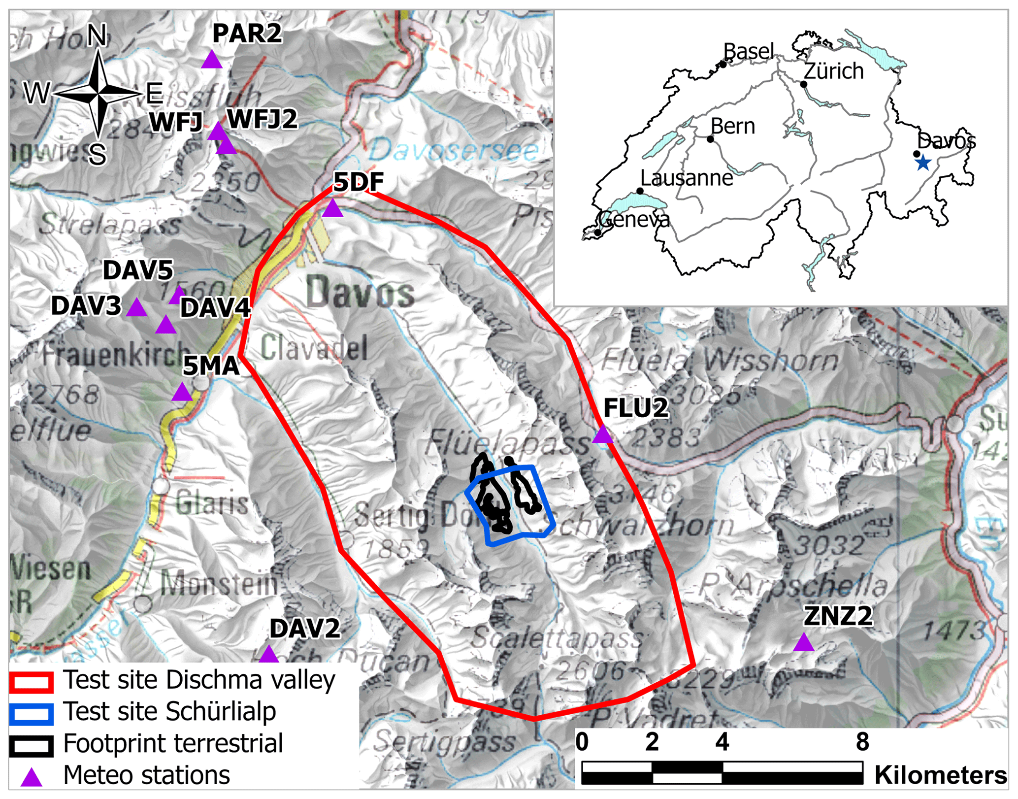
Figure 1 Overview of the test sites: area recorded by the satellite and airplane imagery (red), area covered by the UAS imagery (blue) and area covered by the terrestrial images (black). The purple triangles represent the location of automatic and manual snow measuring stations around Davos. The abbreviations correspond to the snow measuring stations shown in Fig. S1. The blue star in the inset map shows the location of the Schürlialp test site (Swiss Map Raster, source: Federal Office of Topography).

3 Platforms and data

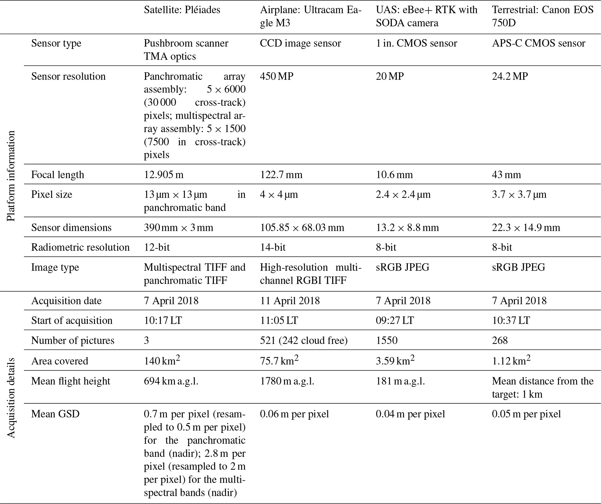
By acquiring satellite, airplane, UAS and terrestrial data over a short time frame (6 d), a comprehensive dataset bringing together small- and large-scale photogrammetric platforms is available for intercomparison. The satellite constellation (Pléiades) consists of two very high-resolution optical satellites with proven performance to derive DSMs (Stumpf et al., 2014). The airplane platform (Ultracam Eagle M3) is a digital aerial large-format camera for state-of-the-art high-resolution aerial photogrammetry. The UAS (eBee+ RTK) is a fixed-wing survey drone equipped with a high-resolution camera and a dual-frequency differential global navigation satellite system (DGNSS) sensor capable of Real-time kinematic (RTK) positioning, all contributing to the delivery of very accurate digital surface models (Benassi et al., 2017). The camera used to capture terrestrial data is a digital single-reflex (SLR) Canon 750D. With this set of photogrammetric platforms, the ground sampling distance (GSD) ranges from 0.04 m per pixel (UAS) to 0.5 m per pixel (satellites). To achieve the consistent geolocation of satellite data and airplane data, independent ground control points (GCPs) and checkpoints (CPs) were collected around Davos during summer. They consisted of features such as roof corners, bridges and other clearly distinguishable man-made features. However, many of these points are not visible in all imagery, either because they are covered by snow in winter or because of challenging interpretation due to the spatial resolution (Pléiades). Therefore 10 additional control points were distributed throughout Dischma, six of them at the test site Schürlialp. Seven of the GCPs were laid out on 6 April and three more on 7 April. They consisted of 0.8×0.8 m white tarps with a black cross and a white square in the middle. The positions of all GCPs were determined using a DGNSS (Trimble Geo XH 6000) with a horizonal and vertical accuracy of 0.1 m. In the following subsections, we present each platform and the corresponding data.

3.1 Satellite: Pléiades

A cloud-free Pléiades-1B stereo image triplet was acquired on 7 April 2018 between 10:17 and 10:19 LT. The panchromatic and multispectral bands (red–green–blue, RGB; near-infrared, NIR) of the Pléiades very high-resolution sensor achieve a spatial resolution of 0.5 and 2 m, respectively. The 12-bit radiometric resolution of Pléiades imagery provides a dynamic range capable of resolving contrast in dark shaded areas as well as across highly reflective snow surfaces. From 694 km above ground, the image triplet was acquired along a descending orbit tracking in eastern Switzerland (across-track incidence angles of 17.4, 12.1 and 9.7^∘, respectively). Along-track incidence angles of −16.3, 7.6 and 17.9^∘ resulted in three stereo pairs with base-over-height ratios (B∕H) of 0.42 (images 1 and 2: pair P12), 0.19 (images 2 and 3: pair P23) and 0.62 (image 1 and 3: pair P13). Although both P12 and P13 have B∕H recommended for photogrammetric work (>0.25; Astrium, 2012), P23 is below the usual standard to process an accurate DSM due to acute parallax angles. Meanwhile, larger B∕H ratios, such as stereo P12, can yield unresolved areas due to terrain obstruction in steep topography. In addition, complicated parallaxes can modify the appearance of ground features and in turn challenging stereo-matching. For this study, we processed the three stereo pairs and considered occlusion and accuracy of each DSM to create a single merged surface product, as explained in Sect. 4.2.

3.2 Airplane: Ultracam Eagle M3

Airborne imagery was acquired with an Ultracam Eagle M3 by the company Flotron on 11 April 2018 between 11:00 and 12:00 LT. Unfortunately, the data could not be acquired on the same day as the satellite triplet due to technical issues on the airplane. The meteorological conditions during the data acquisition were partly cloudy, and only the northern part of the Dischma valley was cloud free. From 512 images, only 242 images could be used for photogrammetric processing. Fortunately, no noticeable snowfall event occurred between 6 and 11 April 2018, and the temperature was too low to allow for significant snowmelt (maximum 10 cm between 6 and 11 April at the low-elevation stations; see graph in Fig. S1). The Ultracam Eagle M3 features a large-format charge-coupled device (CCD) image sensor with 450 megapixels (MP) and a pixel size of 4 µm×4 µm (see Table 1 for more information). The Ultracam Eagle M3 was mounted with the 122.7 mm focal length lens and flown at a mean altitude of 1780 m above ground level (a.g.l.), resulting in a GSD of ca. 6 cm per pixel. The Ultracam Eagle M3 images were recorded with a 14-bit radiometric resolution. The images delivered were four-band (RGB and NIR) geotagged images. Furthermore, the data were delivered with camera positions and orientations with a DGNSS accuracy of 0.2 m and an inertial measurement unit (IMU) accuracy of 0.01^∘ (omega, phi, kappa) and corrected for lever arm and boresight calibration.

3.3 UAS: eBee+ RTK with SenseFly S.O.D.A. camera

UAS imagery of the Schürlialp area was collected on 7 April 2018 at 09:27 LT for 1.5 h (three flights) with an eBee+ RTK of SenseFly equipped with the S.O.D.A. camera. This imaging payload features a 1 in. complementary metal–oxide–semiconductor (CMOS) sensor with 20 MP (see Table 1 for more information) built specifically for photogrammetric applications. The images were recorded in the JPEG format with 8-bit radiometric resolution for each channel. Flying at 182 m a.g.l. on average with lateral and forward overlaps of 70 % and 60 %, respectively, yields 1550 images with an average GSD of 0.04 m. A characterizing feature of the eBee+ RTK is the onboard DGNSS, which measured the camera positions with a mean horizontal accuracy of ca. 0.02 m and mean vertical accuracy of ca. 0.03 m. For RTK operation, the eBee+ RTK was referenced directly in the Swiss coordinate system LV95LN02, relative to mount point VRS_GISGEOLV95LN02 of the national DGNSS network.

3.4 Terrestrial: Canon EOS 750D

The terrestrial images were collected manually on a tripod with a Canon EOS 750D SLR camera on 7 April 2018 starting at 10:37 LT for 1 h. The Canon EOS 750D is a digital SLR camera featuring an APS-C CMOS sensor with 24.2 MP resolution. We used a zoom lens (18–55 mm) and set the focal length at 43 mm. We chose the focal length of 43 mm as a compromise to achieve a mean GSD in the range of the other platforms for the selected camera locations. To ensure stable recording conditions, a tripod was used to take pictures from five different vantage points. The tripod was placed at each location, and the camera was rotated on the tripod head. The entire set-up was moved in one piece so that the focal length stayed fixed. To document the camera location, the DGNSS (Trimble Geo XH 6000) was placed on the top of the camera, and this position was measured with a horizontal and vertical accuracy of 0.1 m. The GSD of this terrestrial recording changes strongly across the slope, which affects the photogrammetric results. In order to achieve accurate measurement in all directions, the ray intersection angle is optimal around 90 to 100^∘, which requires a sufficient B∕H ratio (Luhmann et al., 2014, p. 547), while also promoting terrain occlusions, making terrestrial recording challenging. With the camera positioned at the bottom of the Dischma valley, some slopes to the south-west and to the north-east are more than 1 km away. Thus, the GSD varies between 0.01 m per pixel and 0.1 m per pixel with a mean GSD of 0.05 m per pixel. Towards the north and south sides, the flat valley floor is not suitable for snow depth mapping. A total of 268 images were recorded on 7 April 2018 with 8-bit radiometric resolution in JPEG format, covering the slopes of the northern part of the Schürlialp test site (see Fig. 1).

Table 1 Summary of the photographic data collection with the satellite, airplane, UAS and terrestrial platforms.

3.5 Reference datasets

Manual snow depth measurements and fixed snow depth poles

Manual snow-probing measurements at 27 locations at the Schürlialp test site were performed on 6 April (17 measurements) and 7 April 2018 (10 measurements). The automatic stations around Davos (Fig. 1) measured a decrease in snow depth of 0.04 m between these 2 d at the lowest-elevation station Davos Flüelastrasse (5DF; 1560 m a.s.l.). For each snow probing location, the snow depth was measured plumb with an avalanche probe at each corner and in the middle of a 1×1 m square. The position of the square centre was recorded with a DGNSS (Trimble Geo XH 6000). As manual snow probe measurements are only possible in terrain safe from avalanches, 15 fixed snow poles were installed throughout the Schürlialp area in summer (see Fig. 2). The snow depths values were read off the poles with binoculars or zoomed photos. The snow poles were marked every half metre by pointer and red tape at every 0.1 m, allowing a measuring accuracy of ca. 0.05 m (see Fig. 2). We estimate this uncertainty because a small depression often exists around the pole, and it is possible that the snow pole is slightly tilted by the snow load. At the time of the campaign, the snow depth could be read from 10 snow poles. The other five poles were not visible due to a lack of contrast against the snow or avalanches that bent them previously.

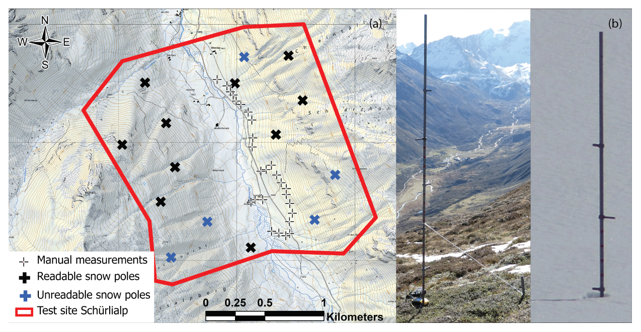
Figure 2 Panel (a) shows the distribution of the snow poles and the manual snow measurements at the Schürlialp test site. The snow poles are separated into the readable (black crosses) and unreadable ones (blue crosses). The thin black crosses show the locations of the manual measurements. The two images in (b) show a snow pole in summer and winter. The snow poles have a hinge at the foot and are tensioned back with a nylon cord. This way they simply fold down in the event of an avalanche and are not dragged along (Swiss Map Raster, source: Federal Office of Topography).

3.6 Summer reference datasets

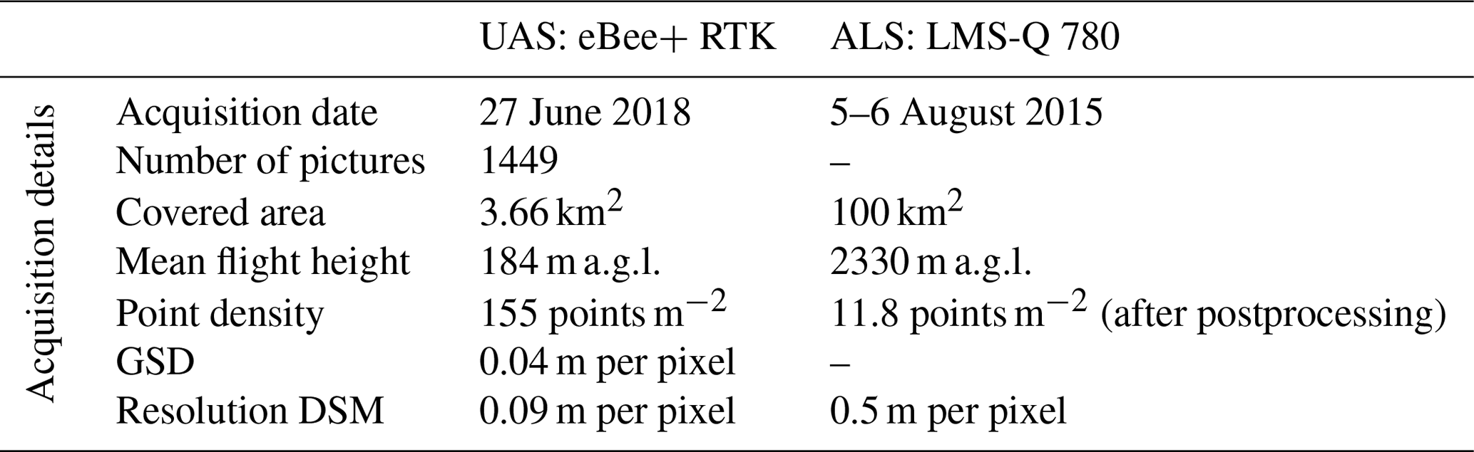
Mapping snow depth requires an accurate snow-free reference surface. For this study two completely snow-free summer DSMs were considered. For the snow depth maps of the Schürlialp test site, a UAS (eBee+ RTK) flight was performed on 27 June 2018, yielding a final DSM with spatial resolution of 0.09 m. For further information about the processing workflow see Sect. 4.4. For producing snow depth maps extending beyond the Schürlialp test site, a DSM with a spatial resolution of 0.5 m derived from an airborne laser scan (ALS) of the Dischma valley was used. The flight covered the Dischma valley but not the entire area captured by the satellite and airplane imagery. The ALS flight was conducted on 5 and 6 August 2015 by Milan Geoservice GmbH with a Riegl LMS-Q 780 scanner. Milan Geoservice GmbH delivered an oriented, unclassified point cloud in the reference system LV03 LN02. Ground point classification and DSM generation were done using the software LAStools (Isenburg, 2014).

Table 2 Description of the summer datasets used for the calculation of the snow depth maps.

4 Data processing

Before a photogrammetric snow depth map or an orthoimage can be generated, a DSM must first be produced from the images of each platform. We used the software packages Agisoft Metashape version 1.5.3/1.5.5 (for airplane, UAS and terrestrial data) and a combination of ERDAS Imagine 2018, Ames Stereo Pipeline (ASP 2.6.2) and GDAL (GDAL/OGR contributors, 2020) (for satellite data) for photogrammetric triangulation, restitution of DSM and production of orthoimages. Once DSMs and orthoimages were created as raster datasets, snow depth maps were calculated using ArcGIS Pro version 2.4.2 by subtracting the summer DSM from the winter DSM. The resulting snow depth maps were validated and compared using two different strategies in order to evaluate the performance of the individual platforms and workflows. More specific aspects of data processing and performance evaluation are provided in the following sections.

4.1 Coordinate systems

Analysing data in the same horizontal coordinate system with the same vertical datum is fundamental for the calculation of snow depth maps. This requires documentation and verification of the coordinate systems and vertical datums used across the processing workflow for each dataset. For example, the geometry of the satellite imagery is defined in terms of a WGS84 ellipsoid, both for planimetry and elevation (height above ellipsoid, HAE). Other data such as the summer ALS DSM were delivered in the Swiss coordinate system LV03/LN02. All DGNSS data (GCP, UAS) were recorded in RTK mode based on a swipos-GIS/GEO correction stream using the LN02 height system.

Because the conversion from ellipsoidal heights (WGS84) to LN02 is only achieved by means of interpolation, we defined the new Swiss height system LHN95 and the local reference system LV95 as the main reference frame for this study. The height system LHN95 (Landeshöhennetz, 1995) is derived from geopotential number and provides rigorous orthometric heights with consideration of the Alpine uplift (Schlatter and Marti, 2005). However, because of its official and legal status, most of the data in Switzerland are measured in the LN02 height system. Therefore, the datasets were provided either on LN02 or on WGS84, and all conversions from LN02 to LHN95 and WGS84 to LHN95 were handled using the REFRAME library provided by swisstopo. REFRAME was used to create conversion grids to accommodate (i) WGS84 to Bessel ellipsoidal height separation (deterministic calculation), (ii) Bessel to LHN95 separation (CHGEO2004 geoid model) and (iii) LHN95 to LN02 separation (HTRANS).

4.2 Satellite data-processing workflow

Processing of Pléiades satellite images involved triangulation in ERDAS Imagine 2018, surface restitution in NASA Ames Stereo Pipeline (ASP; Shean et al., 2016; Beyer et al., 2018) version 2.6.2 (https://doi.org/10.5281/zenodo.3247734), and DSM postprocessing and production of orthoimagery with custom scripts in GDAL 2.4.1. Satellite image triplet bundle block triangulation (BBA) is best performed on WGS84 to ensure unambiguous rational polynomial coefficient (RPC) modelling. The 14 GCPs from the field survey (see Sect. 3) with coordinates accurate to the decimetre on LV95 and Bessel HAE were converted with REFRAME to UTM32N (ETRS89) and WGS84 HAE. BBA triangulation was completed on the 0.5 m resolution panchromatic images with manual input and manual refinements of the 14 GCPs and 32 tie points to achieve a robust BBA solution. Final quality assessment of the triangulation was derived from leave-one-out cross-validation (LOOCV) (Sirguey and Cullen, 2014), whereby each GCP is set as a checkpoint in turn to generate an independent residual, yielding 0.43 m CE90 (circular error of 90 %) and 0.43 m LE90 (linear error of 90 %).

Dense stereo-matching at full resolution (0.5 m) was completed with ASP using a hybrid global-matching approach (Hirschmuller, 2008; d'Angelo, 2016; Beyer et al., 2018). DSMs were produced from a point cloud at 2 m resolution on UTM32N/WGS84, reprojected to LV95 with GDAL (cubic convolution) and height-adjusted to LHN95 using conversion grids mentioned in Sect. 4.1. Maps of ray intersection errors from stereo-matching with ASP measure the minimal distance between rays for pairwise stereo and are indicative of the quality of the match. In tri-stereo configuration, we generated a DSM and map of ray intersection error for each stereo pair. We blended DSMs with GDAL using a weighted arithmetic mean, whereby the elevation from each constituent DSM was weighted by its corresponding ray intersection error. A map of standard error in the weighted mean was generated by uncertainty propagation. The relatively small B∕H ratio of the pair P23 resulted in significantly higher noise that compromised the tri-stereo blending. Alternatively, blending only DSM members P12 and P13 provided a better surface, with noise comparable to or better than the bi-stereo with the largest B∕H ratio (P13). P23 was only used to fill gaps remaining from the two-member blending. The final DSM was used to orthorectify each of the three images, and the three pan-sharpened orthoimages were then blended together to create a single final orthoimage. Finally, the map of standard error for the blended DSM was used to set all cells of the DSM to no data where the ray intersection error was greater than 1 panchromatic pixel (0.5 m) as larger errors were found to often be indicative of erroneous stereo-matching.

Despite the robust survey quality indicated by LOOCV, a remaining 27.5 arcsec tilt (66.7 ppm, or ±1 m over 15 km) along the north-west–south-east axis of the imagery was detected in the blended DSM after differencing with the summer ALS DSM. To correct the tilt, points were manually placed along snow-free roads in the imagery, and spot elevations were extracted from the blended DSM and ALS surfaces. The distribution of offsets along roads in the city and inside the valley revealed enough linearity to justify the fitting of a plane in 3D space. This hyperplane was fit via least squares through the residuals to create a corrective grid covering the imagery footprint which was used to adjust the blended DSM.

4.3 Airplane data-processing workflow

The Ultracam Eagle M3 images are distinguished by a high dynamic range (14-bit radiometric resolution). We used Agisoft Metashape for image processing, which can be applied for images acquired with RGB- or multispectral-type frame sensors (Westoby et al., 2012) and supports up to 16-bit radiometric resolution. Since the southern part of the Dischma valley was cloud-covered, the images were manually sorted into cloud-free and cloud-covered images. The camera positions delivered in the height system LN02 were converted into LHN95 with REFRAME for input into Agisoft Metashape. The use of the CHGeo2004 geoid model in Agisoft Metashape then allows for consistent processing in the vertical height system LHN95.

The images were imported into Agisoft Metashape and aligned. The Ultracam Eagle M3 is a professional photogrammetric camera that has been accurately calibrated by the vendor so that a refinement of the internal camera parameters by Agisoft is not desirable. Therefore before alignment, the camera parameters were fixed in Agisoft Metashape to a focal length of 122.7 mm and 0.004 mm×0.004 mm pixel sizes (see Table 1). All the other camera model parameters (cx, cy, b1, b2, k1, k2, k3, k4, p1, p2; see Agisoft LLC, 2019 for more information about the frame camera model) were fixed to 0 according to the calibration report of the camera. To improve the geolocation accuracy after alignment, 29 GCPs distributed over the Dischma valley were imported into Agisoft. A total of 15 CPs were used to control the geolocation accuracy (see Sect. 3 for more information about GCP and CP). The CPs resulted in an RMSE value of 0.14 m for the XY coordinates and an RMSE value of 0.19 m for the Z. After alignment and refinement of the geolocation accuracy, the dense point cloud was produced with the depth filtering method “aggressive”. The filtering method “aggressive” gives, in our experience, the best results for snow-covered surfaces and filters out most outliers, leading to cleaner surface models. The DSM was generated from the dense point cloud at a 0.11 m per pixel resolution without interpolating voids. Finally, an orthoimage at a resolution of 0.5 m per pixel was created based on the DSM.

4.4 UAS-processing workflow

The eBee+ RTK has an IMU on board for flight control for which the accuracy and calibration are not given by the manufacturer. Therefore, we have processed the imagery in Agisoft Metashape without IMU but with the DGNSS data only. Since the mount point applied the corrections for the Swiss coordinate system LV95 LN02 during the flight, the camera positions of the eBee+ RTK had to be transformed into the vertical coordinate system LHN95 before processing could take place. This was done by first exporting the camera position of the eBee+ RTK images stored in EXIF metadata to a text file used as input for REFRAME to convert the positions into LHN95 for use in Agisoft Metashape. Again, the use of the CHGeo2004 geoid model in Agisoft Metashape allowed for consistent processing in the vertical height system LHN95. The images were then aligned and georeferenced without GCPs and using only CPs to assess the accuracy of the triangulation. SenseFly, the manufacturer of the eBee+ RTK, claims that this approach of integrated sensor orientation (ISO) can achieve accuracies of the order of 0.03 m horizontally and 0.05 m vertically (level of accuracy of 1 to 3× GSD) (Benassi et al., 2017; Roze et al., 2017). Benassi et al. (2017) showed an RMSE value of 0.02 to 0.03 m for the horizonal coordinates of checkpoints and an RMSE value of 0.02 to 0.1 m for the vertical coordinates of CPs for a flight with RTK solution but without GCPs. We assessed the model accuracy using six of the signalled CPs at the Schürlialp test site, resulting in total RMSE values for XY and Z coordinates of 0.05 and 0.1 m, respectively. A dense point cloud was produced with the filtering mode “aggressive”. Finally, the DSM was created with a resolution of 0.09 m per pixel without interpolation, which was used to produce an orthoimage at 0.04 m per pixel.

The summer eBee+ RTK flight was processed with the same workflow as the winter eBee+ RTK flight. This resulted in a DSM with a resolution of 0.09 m per pixel and an orthoimage of 0.04 m per pixel. Six CP markers were signalled on the ground for the summer eBee+ RTK survey and measured with a Stonex S800 receiver and S4II Win Mobile 6.5 controller providing accuracy for the horizontal position between 0.014 to 0.022 m and a vertical position accuracy of 0.02 m. Photogrammetric modelling in Agisoft resulted in RMSE values for the XY and Z of 0.02 and 0.05 m, respectively.

4.5 Terrestrial-processing workflow

Terrestrial snow depth mapping is a compromise between measurement requirements and time. Therefore, due to the avalanche situation and the logistical effort that would have been necessary, no control points could be distributed over the area during data capture. The GCPs and CPs used for the satellite, airplane and UAS are not visible in the terrestrial images. Only the camera positions were measured with a DGNSS (see Sect. 3.4) during recording. However, this did not allow us to determine the precise offset between the DGNSS antenna phase and the principal point of the camera. For this reason, the measurement accuracy of the camera position used in Agisoft Metashape was set to 0.2 m.

To refine the georeferencing of the terrestrial images, features such as stones, bushes and house corners emerging from the snow were detected manually on the terrestrial images to serve as GCPs. The features of nine GCPs were then identified on the orthoimage and DSM products from the UAS summer survey from which coordinates were extracted. The images were therefore sorted into the five camera stations in Agisoft Metashape and aligned and georeferenced with GCPs. Again, the dense point cloud was created with the “aggressive” filter and a DSM and orthoimage produced at 0.11 and 0.06 m per pixel, respectively.

4.6 Snow depth map validation and comparison strategies

Three comparison strategies were developed to compare the photogrammetric data and investigate the performance of the different platforms (see Fig. 3). Comparison 1 aims to validate the snow depth maps for the Schürlialp test site using the manual and snow pole measurements (described in Sect. 4.6.1). Comparison 2 compares the different snow depth maps with the spatially dense UAS snow depth map used as spatial reference (described in Sect. 4.6.2). The UAS summer reference is used for calculating the snow depth maps of comparison 1 and comparison 2. Finally, in comparison 3, snow depth maps of satellite and airplane imagery are calculated and compared with the ALS summer scan (described in Sect. 4.6.3) to show the potential of measuring snow depth distribution over larger areas. Section 4.6.4 describes the accuracy measures used within this paper.

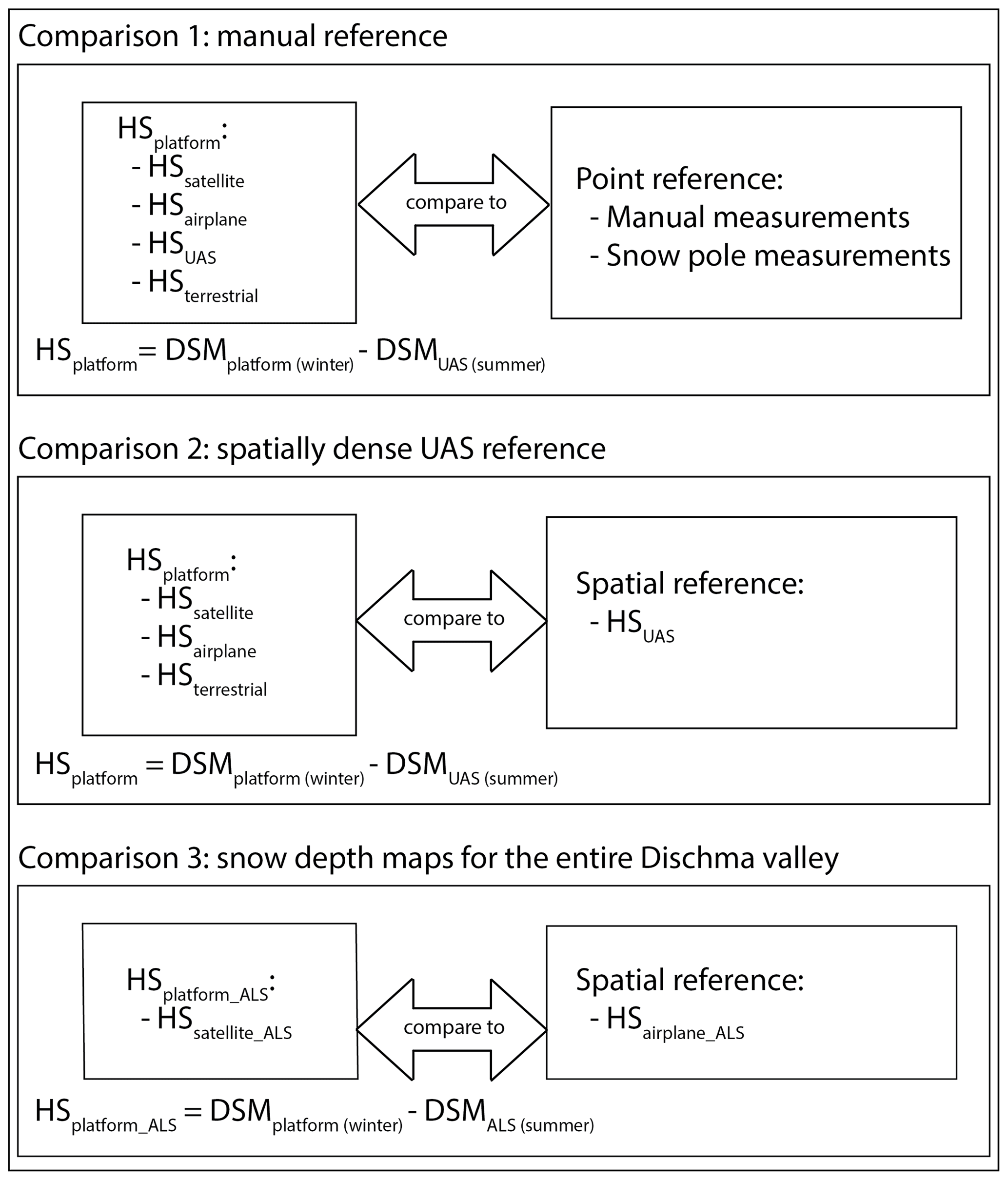
Figure 3 Flow chart illustrating the three comparison strategies. With HS_platform we refer to the snow depth map of the respective platform. HS_{platform_ALS} is the snow depth map of the respective platform calculated with the ALS summer DSM.

4.6.1 Comparison 1: manual reference

For comparison 1 only the Schürlialp (3.59 km²) test site was considered. This provided a detailed comparison of each platform's accuracy against the manual measurements and the snow pole measurements. The snow depth maps are calculated with the UAS summer DSM of 27 June 2018. To keep interpolation errors as low as possible, the winter DSMs were exported at their highest native spatial resolution: satellite DSM at 2 m, airplane DSM at 0.11 m, UAS DSM at 0.09 m and terrestrial DSM at 0.11 m resolution. Prior to generating the snow depth maps, the summer and winter DSMs were made coincident (equal size and winter DSM snapped to summer DSM). The summer DSM was then subtracted from the winter DSM, resulting in the corresponding platform snow depth map. Finally, to compare the snow depth maps from each platform with the manual reference measurements, a buffer with a radius of 0.7 m (i.e. the half-diagonal of the 1 m×1 m sample square) was created from the centre position of the manual measurement. For each snow depth map, the mean value and the standard deviation were calculated within this buffer area. Because the selected buffer has a smaller area than the resolution of the satellite data, the cell value was extracted at the position of the snow depth measurements and the snow poles for this data. In Sect. 4.6.4 further details of the accuracy and precision measures calculated are defined.

4.6.2 Comparison 2: spatially dense UAS reference

The high accuracy of UAS data for snow depth mapping has been successfully tested in various studies (Vander Jagt et al., 2015; Bühler et al., 2016; De Michele et al., 2016; Harder et al., 2016; Cimoli et al., 2017; Redpath et al., 2018; Avanzi et al., 2018; Eker et al., 2019). With comparison 2, we compare the spatially continuous snow depth map of the UAS with the snow depth maps of the other three platforms. Therefore, the winter and summer DSMs of the UAS were exported from Agisoft Metashape at a spatial resolution of 0.11 m (for terrestrial and airplane comparison) and 2 m (for satellite comparison). These DSMs were then aligned to the snow depth maps used in the comparison via cubic-convolution resampling. Finally, the winter DSMs were subtracted from the summer DSMs, resulting in three snow depth maps, with that from the UAS used as reference for comparison 2. With these snow depth maps, the metrics and plots described in Sect. 4.6.4 were calculated.

4.6.3 Comparison 3: snow depth maps of the entire Dischma valley

The summer ALS scan covers a much larger area (100 km²) compared with the UAS summer flight. We calculated the snow depth maps from the satellite and the airplane imagery using the summer ALS scan. We re-exported the airplane DSM at 2 m resolution with Agisoft Metashape. We aligned the satellite and the airplane DSM to the ALS DSM and subtracted the summer ALS DSM from each winter DSM with cubic-convolution resampling. To compare snow depth measurements over a much larger area, we used the airplane snow depth map as a reference to calculate the accuracy and precision of the satellite map.

4.6.4 Accuracy and precision measures

We evaluated the snow depth maps in the different comparisons using a selection of accuracy and precision measures (see Table 3). Accuracy defines how close an estimated value is to a standard or accepted value of a given quantity. Precision (dispersion) on the other hand describes how close measurements agree with each other despite possible systematic bias. The root mean square error (RMSE) is a common measure of accuracy. The standard deviation (SD) is a common measure of precision and measures the dispersion of the data in relation to the mean (Maune and Naygandhi, 2018). To detect systematic vertical offsets of the snow depth maps, the mean bias error (MBE) and the median of the bias errors (MdBE) were calculated. The MdBE is less sensitive to outliers than the MBE, and the difference between the two measures gives an indication of the role of outliers in the metrics. Similarly, the NMAD is a measure of precision that is more robust to outliers than SD (Höhle and Höhle, 2009).

Box plots and normalized histograms were calculated for the first two comparison strategies to illustrate the accuracy assessment by graphical means. The box plot summarizes the statistical measures of the median, quantile, span and interquantile distance that support a graphical interpretation of the results. For the histogram the values were normalized, and the y axis shows the relative frequency of the values. We considered a filtered version of the errors in each platform comparison, whereby errors greater than 2 SDs were classified as outliers and removed. There are different methods described in the literature to remove outliers; one is to remove data in excess of 3 SDs (Höhle and Höhle, 2009; Novac, 2018). We prefer to be more liberal and filtered the data only with a threshold of 2 SDs, where, for normal distribution, 95 % of the values would be found. The accuracy and precision measures as well as the box plot and histogram were calculated again with the filtered data. Additionally, we generated scatter plots for comparison 2 and comparison 3 to illustrate the dispersion in snow depth from satellite, airplane and terrestrial platforms compared to the reference from the UAS platform and calculated the Pearson correlation coefficient (R²). To analyse only the per-pixel value correlation of the snow depth maps in the positive realistic range, we calculate a second scatter plot, where all negative values and values higher than a maximum snow depth (5 m defined by expert opinion and based on the snow depth distribution) of the reference snow depth map are deleted, and the Pearson correlation coefficient (R²) is calculated again. This gives us an indication of how the snow depth maps correlate in the positive and most relevant range for most modelling purposes.

Table 3 Accuracy and precision measures adapted from Höhle and Höhle (2009).

5 Results

The satellite imagery covered 140 km², the airplane imagery covered 75.7 km² in the northern part of the Dischma valley, the UAS imagery covered 3.59 km² around Schürlialp, and finally the terrestrial images covered the smallest area of 1.12 km². The orthoimages in Fig. 4 show the footprint covered by each platform. The orthoimages of both the satellite and UAS are cloud-free, while the orthoimage of the airplane only covers the northern part of the Dischma valley because of clouds. The orthoimage of the terrestrial imagery reveals the suboptimal recording geometry and large terrain occlusions.

The following subsections present the results in detail according to the comparison strategies described in Sect. 4.6. Section 5.1 shows the results of comparison 1. Section 5.2 continues with the results of comparison 2. Finally, in Sect. 5.3 the snow depth maps of the entire Dischma valley are illustrated.

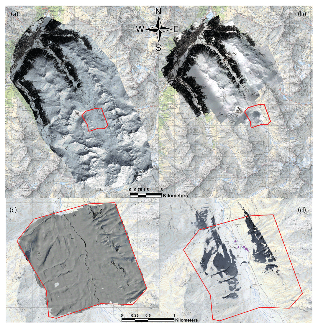
Figure 4 (a) Orthoimage of the satellite data, (b) orthoimage of the airplane data. The area recorded by the airplane is theoretically larger than the area recorded by the satellites, but due to the clouds only part of the images could be used for producing DSM and orthoimagery. (c) The orthoimage of the UAS data and (d) orthoimage of the terrestrial data. The red polygon in (a), (b), (c) and (d) indicates the Schürlialp site test. The violet stars in (d) indicate the five camera positions of the terrestrial recordings (Swiss Map Raster, source: Federal Office of Topography; Pléiades data© CNES 2018, Distribution Airbus DS).

5.1 Results of comparison 1: manual reference

Using the workflows described in the Sect. 4.6.1, a snow depth map was calculated for each platform. The snow depth maps are shown in Fig. 5 and a zoomed inset in Fig. 6. All four maps show similar snow depth distribution patterns, including characteristic snow features such as wind deposits. Figure 6 illustrates how vegetation (here the bush species Alnus alnobetula) can influence the snow depth when using a DSM as summer reference.

The satellite snow depths have the largest dispersion (SD=0.77 m and NMAD=0.43 m) in comparison to the manual and snow pole measurements. The box plots and the histograms (Fig. 7) illustrate the dispersion. The negative MBE (−0.46 m) and negative MdBE (−0.40 m) suggest that the satellite snow depth map is systematically lower compared to the manual and fixed snow pole measurements. After filtering the raw data, the satellite RMSE value is 0.52 m, and the SD is 0.39 m. This improvement can be partially explained by a single large outlier ($\mathrm{\Delta }H=-\mathrm{4.47}$ m) removed with the filter. The satellite snow depth map, however, remains negatively biased at the location of manual and snow pole measurements.

The airplane returns an RMSE value of 0.20 m and the UAS an RMSE value of 0.21 m. Only 27 out of 37 measurements could be considered for the airplane. The SDs of the airplane and the UAS are the same (SD=0.20 m). The NMAD (0.17 m) of the airplane is 0.03 m higher than the one of the UAS (0.14 m), but again the difference is small. The box plot and the histogram illustrate greater dispersion of the errors in the airplane despite the small differences in the accuracy and precision measures compared to the UAS. The MBE (0.03 m) of the airplane is slightly positive, but MdBE (−0.03 m) is negative by the same value. Therefore, we consider this difference of 0.06 m negligible and assume that the airplane snow depth map is not biased. This result is also supported by the box plot for both raw and filtered data. By applying the threshold for outliers, RMSE, SD and NMAD are found to be equal at 0.17 m for the airplane and slightly better (0.11 to 0.16 m) for the UAS. The MBE (−0.07 m) and MdBE (−0.07 m) indicate that the UAS snow depth map has a slight negative bias. This is again consistent with Bühler et al. (2016), who found a slight underestimation of snow depth for UAS. Normally it should be the same for the airplane, but this can be due to the difference in processing as the airplane was processed with GCPs and the UAS without. However, box plots, histograms and accuracy measures of filtered versions of the snow depth maps show that the UAS has the best accuracy compared to manual reference measurement. For the terrestrial snow depth map, only four snow pole measurements could be considered, and therefore the statistical statements are not meaningful. For completeness they are nevertheless listed in Table 4.

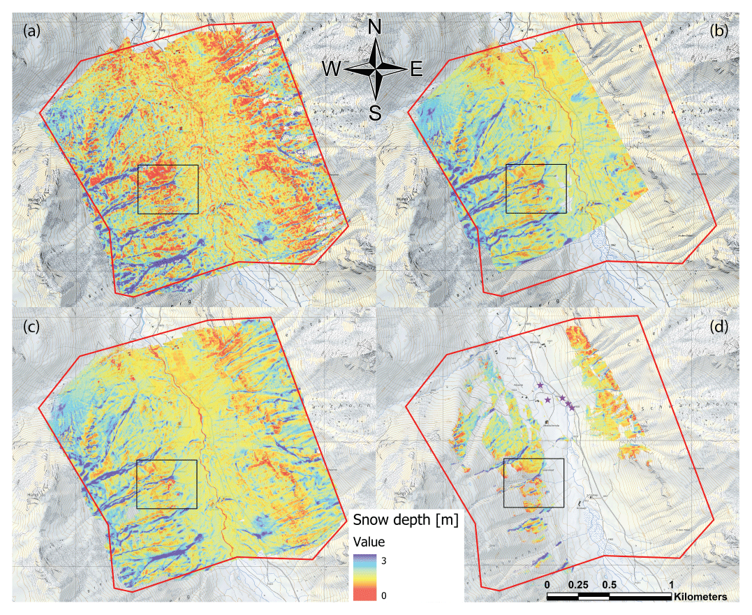
Figure 5 Snow depth maps of the Schürlialp test site from the satellite (a), the airplane (b), the UAS (c) and the terrestrial data (d). On the terrestrial snow depth map, the camera positions are indicated with violet stars. The red polygon depicts the extent of the Schürlialp test site. The black box indicates the zoomed inset shown in Fig. 6 (Swiss Map Raster, source: Federal Office of Topography; Pléiades data © CNES 2018, Distribution Airbus DS).

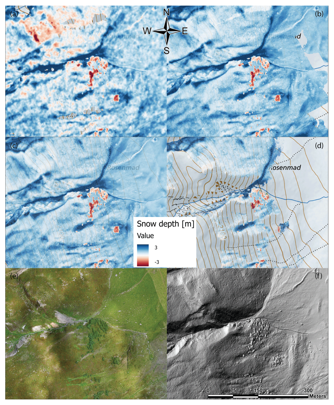
Figure 6 Inset of the Schürlialp snow depth maps shown in Fig. 5, with the scale ranging from −3 to 3 m to illustrate the negative snow depths caused by the vegetation. The effect of bushes (species Alnus alnobetula) under compression by the snow is visible as the greatest negative snow depth values (dark red) in (a) satellite, (b) airplane, (c) UAS and (d) terrestrial snow depth map draped over the swisstopo basemap. An orthoimage for the same extent is shown in (e) from the UAS summer flight and shows a hillshade of the summer ALS scan. Positive snow depth values reach up to 5 m in the gulley features in the study site (Swiss Map Raster, source: Federal Office of Topography; Pléiades data © CNES 2018, Distribution Airbus DS).

Figure 7 Box plots with single-value plots for comparison 1. The orange line depicts the median, the star the mean bias error (MBE). The 25th and 75th quartiles are represented by the boxes and the 5th and 95th percentiles by the whiskers. The left box plot shows the raw data and the right box plot the data where plus or minus 2 SDs are removed. Because of the small sample size of the terrestrial data, applying such a threshold does not have statistical relevance, and therefore the terrestrial data are not shown in the right box plot anymore. To better illustrate the distribution of the error, we calculated single-value plots and included them into the box plots. Note the single large outlier (−4.47 m) from the satellite data is not shown in the raw data to improve interpretation.

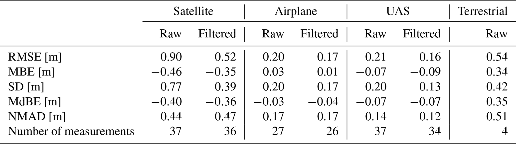
Table 4 A summary of the accuracy assessment of snow depth maps compared to the manual and snow pole measurements for the satellite, airplane, UAS and terrestrial imagery (comparison 1). For the satellite, airplane and the UAS, the threshold of plus or minus 2 SDs was applied, and the updated values are depicted in the column “Filtered”.

5.2 Results of comparison 2: spatially dense UAS reference

Accurate and spatially distributed calculation of snow depth in alpine terrain from UAS imagery has been well documented in recent publications (e.g. Vander Jagt et al., 2015; Bühler et al., 2016; De Michele et al., 2016; Harder et al., 2016; Cimoli et al., 2017; Redpath et al., 2018; Avanzi et al., 2018; Eker et al., 2019) and supported by our results. Comparison 1 confirmed that with an RMSE value of 0.16 m and an NMAD value of 0.11m for the filtered data, the UAS snow depth map is within the expected accuracy for processing with ISO and without GCP. However, due to the rather low number of manual and snow pole measurements, which are also mainly located at the valley floor, the accuracy analysis of comparison 1 may not fully capture the true accuracy of the snow depth products. Therefore, comparison 2 allow us to more comprehensively analyse the performance of satellite, airplane and terrestrial snow depth maps against the entire surface mapped by the UAS winter flight at the Schürlialp study site. The box plot (Fig. 8) shows that all three platforms estimate snow depth within a similar range after filtering the data. Furthermore, the normalized histograms of the raw and the filtered data show that the errors are normally distributed.

Again, the satellite data show the largest error dispersion compared to the airplane and terrestrial data. The box plot and histogram of the satellite data illustrate that the satellite snow depth map is slightly negatively biased over the Schürlialp test site ($\text{MBE}=-\mathrm{0.21}$ m, $\text{MdBE}=-\mathrm{0.19}$ m). After filtering, MBE and MdBE remain negative, with −0.18 m (Table 5). The scatter plot of the satellite data in Fig. 9 also illustrates the lower snow depths from the satellite snow depth map compared to the UAS snow depth map (correlation of R²=0.62).

According to comparison 1, we assume that the airplane snow depth map must correlate strongly with the UAS snow depth map. The MBE and the MdBE as well as the scatter plot confirm this assumption (R²=0.94). The RMSE of the filtered snow depth map from the airplane improved by 0.04 m, from 0.17 to 0.12 m. All other values showed minimal or no improvement when applying the filter. The right box plot in Fig. 8 also displays the low dispersion of the airplane data compared to the UAS data, which is exemplified further by the lower RMSE, SD and NMAD value of 0.12 m for the filtered data.

For the terrestrial data, the snow depth map correlates well with the UAS snow depth map (R²=0.81). The MBE of 0.0 m and the MdBE of −0.02 m show that the terrestrial snow depth map has no overall shift. This is expected since the terrestrial snow depth map was georeferenced with the summer UAS DSM. The box plot (Fig. 8) shows a larger dispersion of the measurements than for the airplane. The filter removed the major outliers, and RMSE (0.21 m), SD (0.21 m) and NMAD (0.19 m) are similar.

Finally, to limit the effects of any outliers we assess the correlation between the satellite, airplane and terrestrial snow depth maps against the UAS snow depth map for values in the range from 0 to 5 m (Fig. 9). The interval from 0 to 5 m was selected based on the snow depth distribution shown in the histogram of Fig. S2. The histogram shows the main snow depth distribution in this range. The results show minimal difference in the correlation for each platform when focusing only on the positive 0 to 5 m snow depth values.

Figure 8 Box plot of comparison 2. The orange line depicts the median, the star the mean bias error (MBE). The 25th and 75th quartiles are represented by the boxes and the 5th and 95th percentiles by the whiskers. The upper-left box plot shows the raw data and the upper-right box plot the data where plus or minus 2 SDs are removed from the raw data. To better illustrate the distribution of the error, we calculated normalized histograms for the raw and filtered data. The bottom-left plot shows the raw data and the bottom-right plot the filtered data.

Table 5 Accuracy and precision assessment for comparison 2: the column “Raw” contains the accuracy measures for all the values, and the column “Filtered” shows the results of the accuracy measures where any values exceeding the threshold of plus or minus 2 SDs are removed. For the satellite data, 4.2 % of the data were removed with the filter, while 4.9 % of the airplane data and 4 % of the terrestrial data were removed.

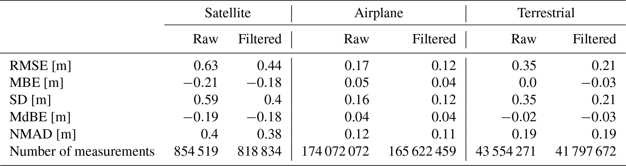
Figure 9 Scatter plot of comparison 2: the three upper scatter plots show the platform snow depth on the x axis and the corresponding UAS snow depth on the y axis. For the lower scatter plots, only the snow depths of the UAS snow depth map in the range of 0 to 5 m were considered and compared to the corresponding values from each platform; 0.8 % of the satellite data, 0.8 % of the airplane data and 1.9 % of the terrestrial data were removed. The scatter plots have a logarithmic scale, which is shown on the right side with a plasma colour bar. R² is given for each scatter plot.

5.3 Result of comparison 3: snow depth maps of the entire Dischma valley

A large-area, high-resolution snow depth map would be of great value for many different applications. Therefore, we produced a snow depth map of the entire Dischma valley with the summer ALS surface as a reference for the winter satellite and airplane DSMs (Fig. 10). Based on the performance in comparison 1 and comparison 2, we use the airplane data to assess the accuracy of the satellite snow depth map. We have a high RMSE (2.2 m) and SD (2.2 m) (summarized in Table 6) as well as a large difference between MBE (−0.02 m) and MdBE (−0.18 m) when using all data. After filtering, the RMSE (0.92 m) and SD (0.9 m) reduce considerably.

We found that the satellite and airplane data were well correlated (R²=0.74; see Fig. 12). The correlation was weaker (R²=0.21) when only focusing on the snow depth estimates between 0 and 5 m. This can be partially explained by the slight negative bias of the satellite snow depth shown by the MBE (raw: −0.02 m; cleaned: −0.17) and the MdBE (raw: −0.18 m; filtered: −0.19 m). This bias is also visible graphically in the box plot (Fig. 11) as well as in the scatter plot (Fig. 12). The normalized histograms (Fig. 11) show that the errors are normally distributed.

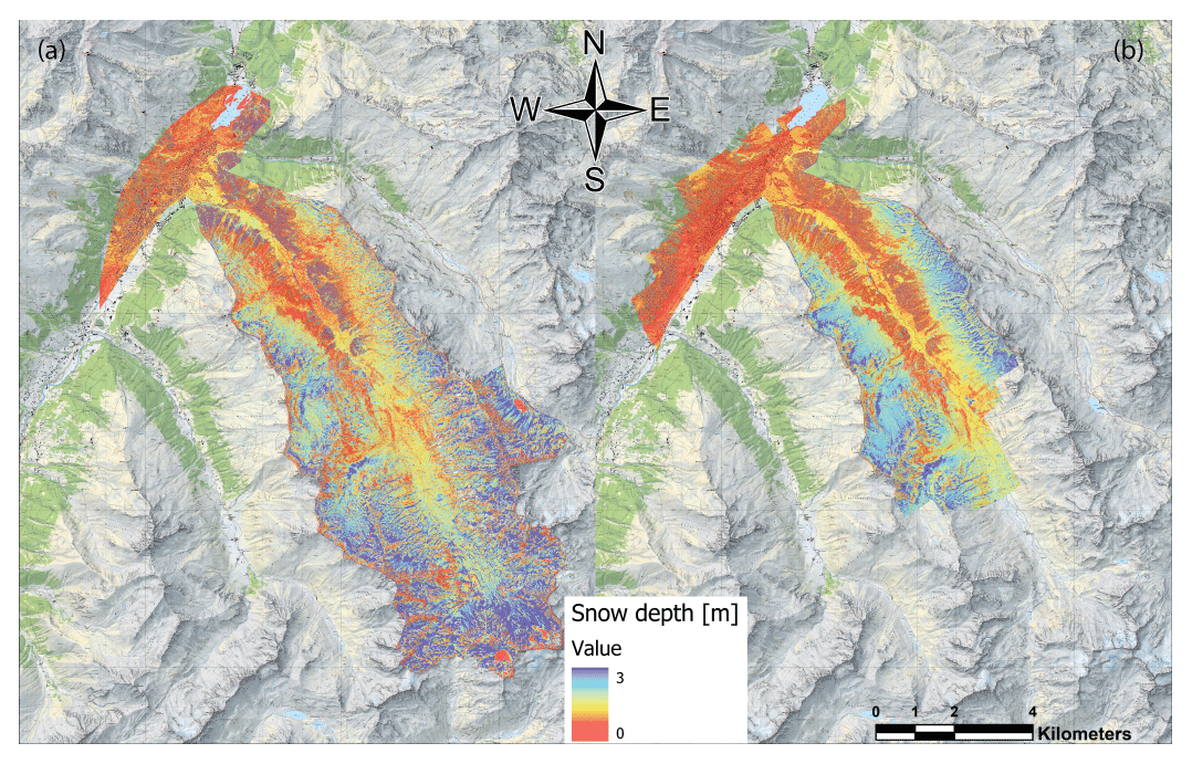
Figure 10 Snow depth maps of the satellite (a) and the airplane (b) platforms for the whole Dischma valley. The snow depth ranges from 0 m (red) to 3 m (blue) based on the summer ALS reference surface (Swiss Map Raster, source: Federal Office of Topography; Pléiades data © CNES 2018, Distribution Airbus DS).

Table 6 Accuracy and precision assessment for comparison 3, where the satellite data are assessed against the airplane data: the column “Raw” contains the results for all the values and the column “Filtered” the results where plus or minus 2 SDs are removed. The filter removed 3.5 % of the data.

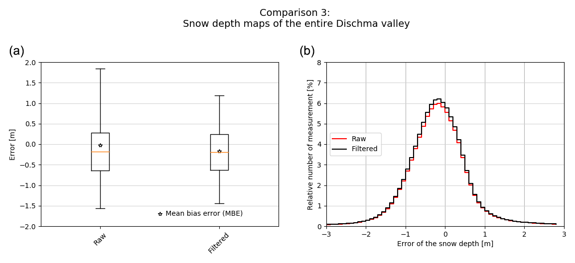
Figure 11 Box plot of comparison 3, the satellite data assessed against the airplane data. The orange line depicts the median, the star the mean bias error (MBE). The 25th and 75th quartiles are represented by the boxes and the 5th and 95th percentiles by the whiskers. The left box plot of the box plot graph illustrates the raw data and the right box plot the filtered data where plus or minus 2 SDs are removed. To better illustrate the distribution, the right plot shows a normalized histogram of the raw and the filtered data.

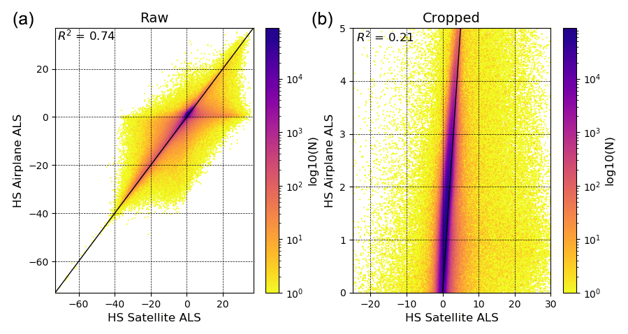
Figure 12 Scatter plot for comparison 3, where satellite snow depth is compared to the airplane snow depth. The left scatter plot shows all data. The right scatter plot shows only the snow depth estimates where the airplane snow depth is between 0 and 5 m. This cropping removed 21.27 % of the data. The scatter plots have a logarithmic scale, which is shown on the right side with a plasma colour bar. R² is given for each scatter plot.

6 Discussion

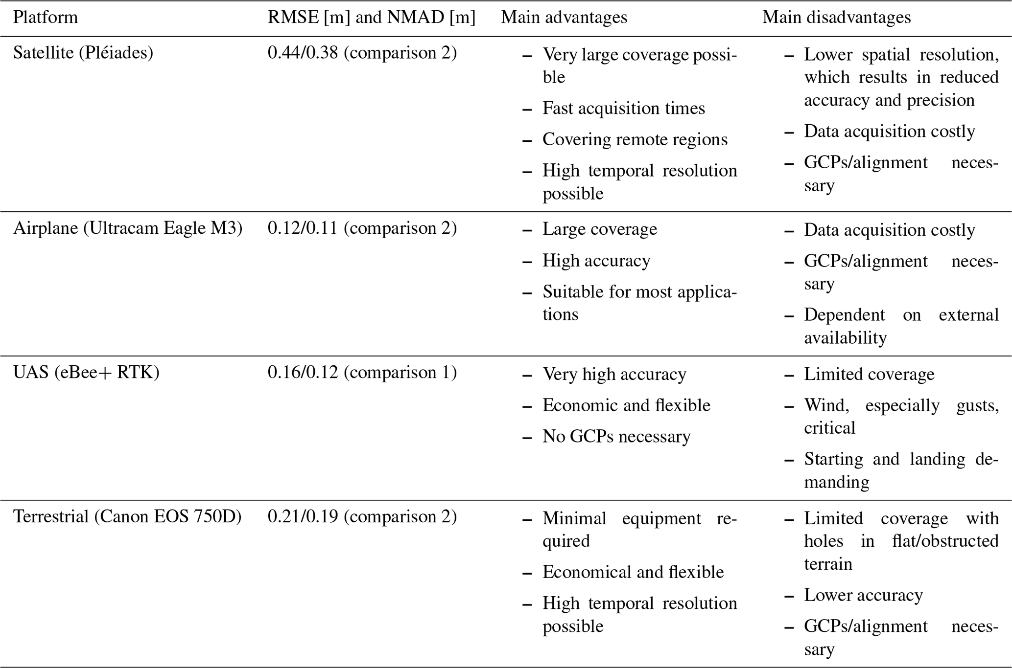
In this study we compare four different photogrammetric platforms, focusing on their performance for spatially continuous snow depth mapping in alpine terrain. Each platform has unique advantages and disadvantages, which we summarize in Table 7. In this section we discuss the results from the three comparisons and describe our experiences using these platforms. We conclude by providing recommendations on potential applications of the platforms.

6.1 Satellite photogrammetry: Pléiades

Very high-resolution optical satellites (GSDs of 0.3 to 0.7 m) have the main advantage that they can image several hundred square kilometres from a single acquisition under cloud-free conditions. Few studies have investigated the performance of satellites for snow depth mapping in alpine terrain. Marti et al. (2016), with a Pléiades snow depth map at a resolution of 2 m, achieved an SD of 0.58 m and an NMAD value of 0.45 m in comparison to manual snow probing. By comparing the same snow depth map to a UAS snow depth map, they calculated an SD of 1.47 m and an NMAD value of 0.78 m. Shaw et al. (2020) found an NMAD value of 0.36 m and an RMSE value of 0.52 m for a snow depth map of 4 m resolution compared to terrestrial lidar. Finally, Deschamps-Berger et al. (2020) achieve an RMSE value of 0.8 m and an NMAD value of 0.69 m in comparison to airborne lidar snow depth maps covering an area over 137 km² at a resolution of 4 m. Also, they performed filtering operations, and in their Pléiades snow depth maps they set snow heights lower than −1 m and higher than 30 m to no data. In this investigation we achieve an RMSE value of 0.63 m (0.44 m filtered) and an NMAD value of 0.4 m (0.38 m filtered) in comparison to a UAS snow depth map Our multi-platform validation was limited to an area of 3.6 km² at the Schürlialp test site, and the comparison methods used in these studies are not all the same. Our snow depth maps are always calculated with an identical summer reference, so we only compare and validate winter DSMs.

Our nested validation method (with probe measurements in comparison 1 to UAS surface in comparison 2 to airplane surface in comparison 3) provides a multi-scale approach to assessing accuracy and precision of photogrammetrically derived snow depth maps. Although we know that the airplane product appears highly accurate and precise over the Schürlialp test site, we could not validate it over the entire valley. It is also important to note some limitation associated with the triangulation of the satellite imagery. Most of the GCPs were collected in summer and only a few could be identified and placed when the images of the satellites were acquired. This compounds with uncertainty in the placement of the GCPs due to the resolution of the imagery. The remaining tilt was assessed and corrected on the basis of points along the roads in three valleys (Sertig, Dischma, Flüela) but without regards to the Schürlialp test site in particular. Thus, the shift does not characterize the technology but shows a limitation of the absolute-orientation approach for snow-covered images.

A photogrammetric challenge also arises from stereo-matching in low-contrast snow-covered surfaces, which combines with imaging geometry and the relatively coarser spatial resolution of satellite imagery, decreasing signal-to-noise ratio in the DSM. This is exacerbated by the lower B∕H ratio (P23 in particular), which led to substantially greater noise in smooth, undisturbed areas of the snowpack. Lower contrast appeared to promote variability in stereo-matching, which compounds with lower parallactic angles when B∕H decreases, thus increasing the dispersion in the triangulated heights in poorly textured areas. With some contrast or texture in the snow (e.g. avalanches deposits), stereo-matching then performed similarly across every stereo pair with no substantial differences in surface height dispersion. This indicates that image contrast and B∕H ratio combine to govern the dispersion of the restitution. An in-depth study may be desirable to characterize this effect further, including testing more stereo-matching options and satellite geometry in such environments.

Our testing shows that given the resolution of the Pléiades imagery, the uncertainty in snow depth retrieval makes the mapping of shallow snowpacks challenging, with mean snow depth values in the range of 0.5 m (Sturm et al., 2008). In mountain regions on the other hand, where larger mean snow depth values are present, and the amplitude of the values is generally larger, satellite-based snow depth maps will provide important estimates of snow distribution. Typical applications that could benefit are the mapping of snow avalanches (Bühler et al., 2019) and the estimation of water resources stored in snow (Jonas et al., 2009) for drinking water supply or hydropower (Farinotti et al., 2012). In many remote regions of the world, where access is difficult and dangerous, satellite photogrammetry proves to be a competitive method to gather spatially continuous snow depth information even though the achievable accuracy is limited.

6.2 Airplane photogrammetry: Ultracam Eagle M3

Airplane photogrammetry campaigns depend on the availability of suitable airplanes and camera systems as well as flight permissions. Entire catchments of several hundred square kilometres can be covered within 1–2 h of flying, with ground sampling distances of 0.05 to 0.25 m. Despite today's availability of high-end camera systems, only few studies have used airplane photogrammetry for snow depth measurements. The investigations of Bühler et al. (2015) and Boesch et al. (2016) with an ADS80/100 optical scanner and Nolan et al. (2015) with a Nikon D800E frame camera reported accuracies of 0.10 to 0.3 m. In our study we use an Ultracam Eagle M3 frame camera and achieve an RMSE value of 0.12 m (0.17 m raw) compared to the UAS snow depth values.

Table 7 Summary of the RMSE and NMAD values and main advantages and disadvantages of the investigated photogrammetric platforms. The reported RMSE and NMAD values for the satellite, airplane and terrestrial data are based on the filtered values from comparison 2. The RMSE and NMAD values shown for the UAS are the filtered values from comparison 1.

Aerial photogrammetry allows for snow depth mapping at a higher spatial resolution than satellite photogrammetry with accuracies close to UAS photogrammetry. This is particularly the case if low flying heights above ground are planned, resulting in higher GSDs of 0.05 to 0.1 m. However, in alpine terrain the GSD varies a lot due to topography as the airplane flight lines are usually at fixed elevations, resulting in varying GSDs within the investigation area. Airplanes can also fly below high clouds; however as for all photogrammetric sensors, diffuse illuminations corrupt the contrast of the snow-covered surfaces and may result in insufficient DSM qualities, resulting in holes and outliers. With high accuracy and precision and the large possible coverage, airplane photogrammetry is a promising tool for all applications where the investigation area is reachable with an airplane, and an accuracy in the range of 0.1 to 0.3 m is acceptable. Also, airborne photogrammetry is costly and depends on GCPs or the alignment to a master scene for orientation. Because of the smaller GSD of the airplane data compared with the satellite data, the accurate photo-identification of points may be easier.

6.3 UAS photogrammetry: eBee+ RTK

UAS photogrammetry has proven to be an accurate, flexible and reliable tool for snow depth mapping, achieving accuracies in the range of 0.05 to 0.2 m (Bühler et al., 2016; Harder et al., 2016; De Michele et al., 2016; Redpath et al., 2018). In this study we applied ISO based on onboard RTK without applying ground control points. Our experience with more than 150 flight missions shows that the snow depth values generated under favourable illumination conditions are of very high quality. Comparison 1 supports this conclusion, which allows us to apply the UAS snow depth map as a reference for the validation of satellite and airplane platforms.

The main limitation of UAS photogrammetry is that current systems cover only a limited area (on the order of a few square kilometres) due to technical limitations. Pilots have to be close to the study site to fly the UAS line of sight. Furthermore, take-off and landing the UAS in high-alpine terrain is challenging, especially if wind gusts of more than 15 m s⁻¹ are present. On the other hand, the UAS enables the flexible generation of accurate and precise DSMs. Therefore, they can be applied for all applications requiring spatially continuous snow depth information as long as a limited area is acceptable. An example for such an application is the measurement of snow redistribution by wind at a specific mountain ridge (Walter et al., 2020).

6.4 Terrestrial photogrammetry: Canon EOS 750D

Terrestrial photogrammetry needs no high-end photogrammetric equipment, and only a consumer camera can be enough to fulfil the task. Therefore, it is a suitable tool if only smaller areas mainly in steep terrain facing towards the cameras should be covered. If fixed-installation cameras are used, a high temporal resolution of several measurements per day is possible. The spatial resolution declines with the distance to the camera position and the inclination away from the sensor. Our results demonstrate that flat regions are often not visible unless you would map from above. A spatially continuous coverage can only be achieved in terrain facing towards the camera. The accuracy and precision achieved in this study ranged from 0.2 to 0.5 m. Terrestrial photogrammetry also encounters limitations such as georeferencing problems, logistic problems or access problems. We performed for example the georeferencing using a UAS flight. This can certainly be avoided with a clear ISO approach and well-distributed GCPs points. But terrestrial photogrammetry remains the most challenging technique because, for a working set-up, access to difficult terrain is necessary (distribution of the GCPs, camera position). Potential applications for such platforms include the mapping of snow avalanche mass balances (e.g. Thibert et al., 2015) or the mapping of snow depth variations at confined locations such as mitigation measures along roads (e.g. Basnet et al., 2016) where large snow depth values are expected.

6.5 Influence of vegetation

Our study confirms the previously noted effect of vegetation on snow depth (Bühler et al., 2016; Harder et al., 2016; Redpath et al., 2018). Photogrammetry-derived DSMs over forested areas have limitations compared with ALS, where above-ground returns can be removed from the surface. Dense vegetation can also produce holes and negative snow depth values in a snow depth map when using photogrammetry. For example, all four snow depth maps showed the same negative snow depth patterns due to the species Alnus alnobetula (Fig. 6). These bushes stand tall (up to 3 m) during summer and are pressed to the ground by the snow cover in winter, resulting in negative snow depth values up to 3 m (Fig. 6). Bühler et al. (2016) have also identified this effect. Feistl et al. (2014) investigated vegetation compression snow and found that, depending on the vegetation type (long grass, short grass and dwarf shrub), the difference between the summer height and the height below snow was between 0.1 and 0.2 m. Our work affirms the utility of ALS for investigating snow depth in densely vegetated or forested areas. Filtering a summer ALS to produce a digital terrain model (DTM) instead of a DSM can improve the snow depth measurements in vegetated areas; however artefacts are likely to remain. Further investigations are needed to quantify the effects of vegetation in estimating snow depth with remote-sensing techniques.

7 Conclusions

In this study we tested and compared a wide range of available photogrammetric platforms for their performance in snow depth mapping. Satellite imagery (Pléiades) demonstrated its capability to map large areas (>100 km²) in a single acquisition but with a lower native spatial resolution (0.5 m) compared with the other platforms. We found an RMSE value of 0.44 m and an NMAD value of 0.38 m for the satellite-derived snow depth map at a spatial resolution of 2 m. The comparison to the UAS (eBee+ RTK) snow depth map demonstrated the high accuracy of the airplane (Ultracam Eagle M3) snow depth map at a high spatial resolution of 0.11 m with an RMSE value of 0.12 m and an NMAD value of 0.11 m. UAS images are an economical and flexible method for mapping snow depth with high accuracy (RMSE value of 0.16 m and NMAD value of 0.11 m) and high spatial resolution (0.09 m snow depth map resolution), but coverage of a UAS is limited. The terrestrial (Canon EOS 750D) platform requires less expensive equipment and supports a high temporal resolution of data capture. However, coverage, accuracy and precision are limited and not possible for every application. The snow depth map of terrestrial images achieved an RMSE value of 0.21 m and an NMAD value of 0.19 m with a snow depth map resolution of 0.11 m.

With these investigations we demonstrate that digital photogrammetry is a powerful tool to map spatially continuous snow depth distribution in alpine terrain. Important applications such as avalanche warning, ecological investigations in alpine environments or hydropower generation can benefit from data acquired by this new technology. With further advancements in sensor technology for all tested platforms, we expect improved accuracies and coverage in the future. Digital photogrammetry may be the preferred method for snow depth mapping as it is more flexible and less costly than laser scanning for most applications as long as the vegetation cover is negligible, and the snow is deep enough.