the Creative Commons Attribution 4.0 License.
the Creative Commons Attribution 4.0 License.
 | 12 Feb 2021
Crystallographic analysis of temperate ice on Rhonegletscher, Swiss Alps
Sebastian Hellmann
Johanna Kerch
Ilka Weikusat
Andreas Bauder
Melchior Grab
Guillaume Jouvet
Margit Schwikowski
Hansruedi Maurer
Crystal orientation fabric (COF) analysis provides information about the c-axis orientation of ice grains and the associated anisotropy and microstructural information about deformation and recrystallisation processes within the glacier. This information can be used to introduce modules that fully describe the microstructural anisotropy or at least direction-dependent enhancement factors for glacier modelling. The COF was studied at an ice core that was obtained from the temperate Rhonegletscher, located in the central Swiss Alps. Seven samples, extracted at depths between 2 and 79 m, were analysed with an automatic fabric analyser. The COF analysis revealed conspicuous four-maxima patterns of the c-axis orientations at all depths. Additional data, such as microstructural images, produced during the ice sample preparation process, were considered to interpret these patterns. Furthermore, repeated high-precision global navigation satellite system (GNSS) surveying allowed the local glacier flow direction to be determined. The relative movements of the individual surveying points indicated longitudinal compressive stresses parallel to the glacier flow. Finally, numerical modelling of the ice flow permitted estimation of the local stress distribution. An integrated analysis of all the data sets provided indications and suggestions for the development of the four-maxima patterns. The centroid of the four-maxima patterns of the individual core samples and the coinciding maximum eigenvector approximately align with the compressive stress directions obtained from numerical modelling with an exception for the deepest sample. The clustering of the c axes in four maxima surrounding the predominant compressive stress direction is most likely the result of a fast migration recrystallisation. This interpretation is supported by air bubble analysis of large-area scanning macroscope (LASM) images. Our results indicate that COF studies, which have so far predominantly been performed on cold ice samples from the polar regions, can also provide valuable insights into the stress and strain rate distribution within temperate glaciers.
- Article
(8920 KB) - Full-text XML
- BibTeX
- EndNote


Since the second half of the last century, ice cores have been regarded as extremely valuable archives for reconstructing the climate history of the past hundreds of thousands of years (Robin et al., 1977; Petit et al., 1999; Thompson et al., 2002). For example, correlations between ice accumulation, isotopes and dust content have been established, but the deformation of ice layers complicates dating and interpretation of climate records (Jansen et al., 2016). Microstructural analyses have been used to overcome these issues (Faria et al., 2010). In addition, microstructural investigations have also been conducted to reconstruct the ice flow of ice sheets in Greenland and Antarctica as well as in glaciated mountain areas (Russell-Head and Budd, 1979; Alley, 1992; Azuma, 1994). For those investigations, the focus has been on the crystallographic orientation of the ice grains. The stresses and strain rates occurring within the ice mass not only cause glacier flow but also induce the development of a characteristic crystal orientation fabric (COF) and microstructural anisotropy (Gow and Williamson, 1976; Herron and Langway, 1982; Alley et al., 1995, 1997) and are summarised in Faria et al. (2014a).
During the past decades, COF and texture have been investigated intensively on polar deep ice cores to understand the microstructure of polycrystalline ice in the context of its deformation history (Hooke, 1973; Gow and Williamson, 1976; Thorsteinsson et al., 1997; Patrick et al., 2003; Gow and Meese, 2007; Pettit et al., 2007; Montagnat et al., 2014; Pettit et al., 2011; Weikusat et al., 2017). A historical summary of these projects can be found in Faria et al. (2014a). For the selected ice core drilling spots on domes and ridges, vertical compression and horizontal extension within the ice mass have been found to be the dominant driving stress for ice deformation. In contrast, for ice samples from temperate glaciers, the deformation is dominated by a series of interfering and changing compressional, extensional and shear stress conditions along the valley. Together with diagenesis, burial, basal sliding and potentially partial melting, these stress conditions result in a much more complex deformation history (Hambrey and Milnes, 1977). This requires more extensive analyses of COF.
The ice of temperate glaciers is comparable with a metamorphic rock close to its melting point (Hambrey and Milnes, 1977) that has been exposed to a long series of deformation processes along the valley. This deformation is caused by various shear and compressional stresses that have been applied to the ice. These stress regimes produce heterogeneously distributed dislocations, which cause dynamic recrystallisation by rearrangement of these dislocations and by internal strain energy reduction. The resulting recrystallisation processes and the interplay between deformation and recrystallisation in the ice take place even faster as the temperature gets closer to the pressure melting point (Alley, 1988; Weikusat et al., 2009a). As a result, the adaption of the ice crystal structure to new stress conditions is expected to be faster (e.g. Kamb, 1972; Duval, 1979). Additionally, the higher temperatures provide more thermal energy and allow a faster grain growth (Azuma et al., 2012), leading to an interplay between stress and temperature regime (Alley, 1988; Faria et al., 2014b). Therefore, large differences can be observed between cold and temperate ice. One of the most apparent differences is the grain size, which has been found to be a few centimetres in temperate ice (Rigsby, 1960), whereas samples from polar ice usually show grains with a diameter of a few millimetres, except in the deepest parts, where temperatures rise close to the pressure melting point (e.g. Gow and Williamson, 1976; Thwaites et al., 1984; Kuiper et al., 2020).
The first crystallographic investigations were already performed on temperate glaciers in the 1950s to 1980s, including the detailed investigations of Kamb (1959) and Rigsby (1960), and later extended by Budd (1972), Hambrey and Milnes (1977), Hooke and Hudleston (1978), and Hambrey et al. (1980). A potential problem of temperate glacier crystal analysis is the large grain size and thus limited number of grains that can be analysed for each sample. This may be the reason why a surprisingly low number of papers have been published on crystal structure of temperate glaciers (e.g. Tison and Hubbard, 2000) during the past years. Furthermore, the majority of the earlier studies mainly analysed samples from the uppermost few metres. To date, ice core drilling and preparation of thin sections is still a time-consuming process. Only a few discrete measurements are possible within a reasonable amount of time. Nonetheless, the technique for analysing COF has developed extensively, for example, by using image analysis software and powerful computing resources (Wilson et al., 2003; Peternell et al., 2009; Wilson and Peternell, 2011; Eichler, 2013).
In this study, we analyse ice core samples from a temperate alpine glacier. We describe and compare our findings with previous studies and provide a hypothesis for the resulting COF in terms of given stress and temperature conditions. We analyse the stress regime in the vicinity of the ice core, using additional borehole measurements, and discuss recrystallisation processes and grain growth in temperate ice. For selected examples we take a closer look at the development of new ice crystals under the current stress regime of the glacier. The microstructural results of this study serve as a basis for geophysical experiments on ice core samples, and they can also be compared with results from larger-scale geophysical experiments.
The fieldwork was carried out on Rhonegletscher, located in the central Swiss Alps (Fig. 1). This glacier currently covers an area of about 15.5 km2 and flows in a southern direction from 3600 down to 2200 It is a medium-sized valley glacier and is easily accessible, and therefore investigations have already been carried out in the last 2 centuries and continuously since 2006 (Bauder, 2018).

Figure 1Rhonegletscher ablation area. Ice core position indicated in red; ice flow direction at ice core location shown by black arrow. Map source: Swiss Federal Office of Topography.
In August 2017, we drilled an ice core in the ablation area of the glacier (Fig. 1), approximately 500 m north of its current terminus. Here, the ice was flowing with an average surface velocity of 16.2 m a−1 in the season 2017/18 according to global navigation satellite system (GNSS) measurements. This location was selected because the glacier surface forms a relatively even plateau with only a 5 m elevation change over a distance of 40 m and is free of crevasses. Further up-glacier there is a steep and crevassed area. An analysis of the bedrock with ground-penetrating radar measurements also confirmed a transition from a steep to a more flat zone of the valley (Church et al., 2018) at the ice core location.
As the ice is just at the pressure melting point, we used a thermal drilling technique (Schwikowski et al., 2014). Although hot-water drillings, performed in the vicinity of the ice core location, showed a mean ice thickness of 110 m, we stopped drilling at 80 m, when hitting some gravel. This gravel blocked the cutter head. We retrieved an 80 m long ice core, with a gap between 46 and 50 m due to technical issues.
Due to the thermal drilling technique, which did not apply a rotational force onto the ice core segments, an oriented retrieval of the segments was possible. A freshly drilled segment was manually connected to the previous one, which worked out well for most of the segments. Additional measurements of the Earth's magnetic field, while drilling, could be used in some cases to reconstruct the orientation within a range of ±10∘ when matching of neighbouring segments was not possible.
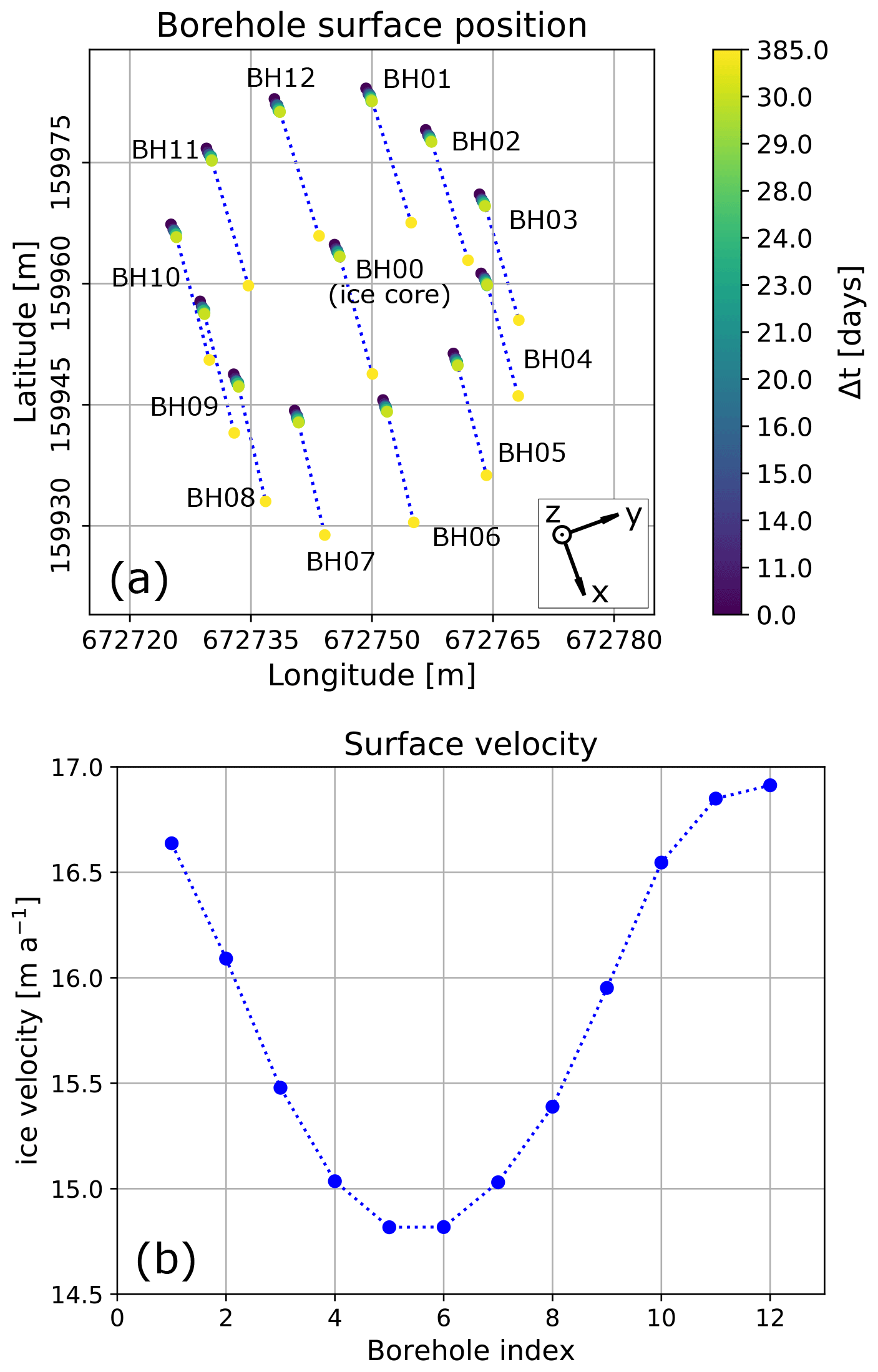
Figure 2Analysis of ice flow direction and velocity for each borehole. (a) The displacement of the borehole surface points measured by GNSS since drilling; inset depicts the glacier flow coordinate system. (b) The absolute surface velocity [m a−1] in the vicinity of each borehole.
To complement the results of the ice core analysis, we made use of an array of hot-water-drilled boreholes surrounding the location of the ice core retrieval (Fig. 2). The locations of the borehole collars were surveyed repeatedly using high-precision GNSS measurements (Fig. 2a). The displacements of the borehole collars indicate a south-eastern flow direction with an azimuth of about 155∘ ± 10∘. We further derived the surface velocities at each borehole location (Fig. 2b). The south-eastern boreholes (BH04 to BH07) show significantly smaller displacements, compared with the boreholes located in the north-western part of the array (BH01 and BH10 to BH12). This indicates compression of the ice in this region, which is expected to lead to larger longitudinal strain rates (convention is that compressional strain rates give negative values). We calculated the surface strain rate components , and (Fig. 3) from these velocities. These strain rates and velocities serve as constraints for the ice flow modelling.
In the following sections, we refer to x as the component in the glacier flow direction (i.e. ≈ 155∘ from the north; see Fig. 1), y as the component perpendicular to the glacier flow (≈ 65∘ from the north) and z as oriented vertically upwards.

To support these observations at the surface, the internal glacier dynamics was investigated by the means of a three-dimensional ice flow model that already existed from previous studies (Jouvet et al., 2009; Morgenthaler, 2019). An updated bedrock model and surface topographic information were used to determine the actual ice thickness of the glacier and to constrain the model. The bedrock model was obtained from GNSS measurements (Church et al., 2018) and from a Swiss-wide glacier inventory that is currently being updated (Farinotti et al., 2009; Grab et al., 2018). With the given information, we simulated the ice flow of Rhonegletscher using the Elmer/Ice modelling code (Gagliardini et al., 2013), which solves the full Stokes equations based on Glen's flow law (Glen, 1955) for the ice rheology; namely,
where is the strain rate, τij is the deviatoric stress and τ is the second invariant of the deviatoric stress tensor. The creep exponent n was set to n=3 as a typical value for valley glaciers (Budd and Jacka, 1989). Basal sliding is modelled by using Weertman's friction law as the boundary condition at the ice–bedrock interface:
where ub is the norm of the basal velocity and τb is the basal shear stress while m=3 and c are constant parameters. The main model parameters are the sliding coefficient c and the rate factor A that control the amount of basal motion and internal deformation, respectively. As the rate factor, we chose A=100 , which was proved to correctly reproduce the velocities of Aletschgletscher (Jouvet et al., 2011). The rate factor is close to the literature value for temperate ice (76 ) (Cuffey and Paterson, 2010). As the sliding coefficient, we used c=10 km MPa−1, which was tuned such that the observed and modelled ice velocities match at the surface of the borehole. Additional sliding velocity values of less than 5 m a−1, estimated from borehole camera investigations (Gräff et al., 2017), support our assumptions for this value. It is rather small compared to previous studies on Alpine glaciers (Jouvet and Funk, 2014; Compagno et al., 2019). Here, we ran the model in a stationary fashion without time evolution. As model outputs, we obtained the velocity and stress field in three dimensions. For a sensitivity analysis, we also tested different rate factors and basal-sliding coefficients. As the model still slightly overestimated the derived basal velocities, we also analysed the case without basal sliding (c=0 km MPa−1). In this case, an extremely high rate factor of A=200 was required to fit the measured velocities. Furthermore, the principal stress axes did not change significantly. These changes led to a slightly enhanced longitudinal simple shear component and slightly weaker longitudinal compressional component in the deepest parts of the ice. Therefore, we only considered A=100 and c=10 km MPa−1 in the following analysis.
For detailed structural investigations of the temperate glacier ice, we performed a COF analysis in the laboratories of the Alfred Wegener Institute Helmholtz Centre for Polar and Marine Research (AWI). We measured the orientation of the c axes of the ice grains. The c axis is the symmetry axis perpendicular to the basal plane of a hexagonal crystal. Along the c axis, the physical properties differ significantly from any direction parallel to the basal plane (the a axes). This results in an anisotropic viscous response of the glacier ice (Schulson and Duval, 2009, chap. 6). Furthermore, the elastic parameters of the ice, such as the bulk or shear modulus, have enhanced values in the c-axis direction and the crystal is more resistant to deformation (Cuffey and Paterson, 2010, chap. 3). This anisotropy affects the elastic properties leading to velocity changes for acoustic waves which travel through the ice (e.g. Diez and Eisen, 2015).
From the ice core extracted from the central borehole BH00 (Fig. 2a), seven samples at depths of 2, 22, 33, 45, 52, 65 and 79 m were considered. Due to technical problems during the core retrieval, the azimuthal orientations of the samples at 2 and 45 m depth are subject to some uncertainties. Their azimuthal orientations were thus obtained from extrapolations from adjacent measurements.
Each of the seven samples consisted of an ice core segment of about 50 cm in length. Up to four 11 cm long adjacent sub-samples (Fig. 4) were prepared from each of these segments. Each sub-sample was then further dissected into a horizontal and two vertical cuts. All three cuts are perpendicular to each other (Fig. 4). This resulted in a horizontal circular slice and two vertical slices with S–N and E–W orientations from which thin sections were prepared. We measured between 8 and 12 thin sections per sample and 77 thin sections in total. This procedure enabled a more comprehensive analysis of the large crystals existing in temperate glacier ice (e.g. Kamb, 1959; Rigsby, 1960) and a tracing of fissures (also called fracture traces), for instance from potential meltwater intrusions. The dimensions of the pieces were 10 × 6 cm for the vertical sections and ∼ 7 cm in diameter for the circular horizontal sections. The creation of sub-samples and choosing three different types of sections (horizontal, E–W vertical, S–N vertical) for every sub-sample resulted in a comprehensive analysis of at least 300 grains for each depth level.
During the preparation of the ice thin sections, we also took large-area scanning macroscope (LASM) images (Binder et al., 2013; Krischke et al., 2015) from the polished surface of the 1 cm thick ice samples. These images provide information on the grain boundary network and subgrain boundaries, as well as on the air bubble distribution, since light from the active camera is backscattered to a great extent by the evenly polished ice surfaces. Uneven parts, such as air bubbles or grain boundaries, reduce the amount of backscattered light and appear darker in the image. All sections were analysed using cross-polarised light (Wilson et al., 2003; Peternell et al., 2009). We used the automatic fabric analyser G50 from Russell-Head Instruments (Wilson et al., 2003) to measure the orientation of the c axis on a predefined mesh grid with a pixel resolution of 20×20 µm2. The orientation of the c axis of an ice crystal is determined by two angles:
The first angle defines the azimuth of the c axis in the horizontal plane. The second angle is the colatitude from the vertical.
For the postprocessing of the obtained crystallographic data, we used the software cAxes (Eichler, 2013). The software analyses the misorientation angle between the determined c-axis orientations of neighbouring pixels and combines those with a misorientation of < 1∘ to individual ice grains with a mean c-axis azimuth and colatitude per grain. The minimum grain size, calculated from the number of pixels multiplied by the pixel resolution, was set to 0.2 mm2 (500 pixels). Next, cAxes automatically rotated the vertical thin sections around the horizontal x-axis x′ of the local measurement coordinate system () by 90∘ so that the vertical component z′ is actually pointing upwards (; see Fig. 4). Then, the thin sections were rotated (with individual angles for the different types of thin sections; see Fig. 4) around the vertical axis z to align them with the glacier flow coordinate system (). In a final step, we used the magnetometer data to correct for offsets between the theoretical and actual azimuthal orientation for the respective thin sections of the individual ice core segments. This step is necessary since some segments have been slightly rotated during retrieval, which we could reconstruct with the respective magnetometer data. This procedure ensured an identical coordinate reference frame for all thin sections along the entire ice core. Finally, we computed the eigenvalue distribution according to the procedure of Wallbrecher (1986). The three eigenvalues λi () follow the relations and . These eigenvalues represent the main axes of an ellipsoid that presents the best fit for a given c-axis density distribution.

Figure 4Cutting scheme for the ice core analysis. An 11 cm long piece of the ice core was cut in a horizontal (d=7 cm) and two vertical (east–west- and south–north-oriented, 10×6 cm) thin sections. Four thin sections of each type were analysed and combined per sampling depth.
Figure 5 shows the results of the COF analysis (left panels) and selected images of horizontal thin sections (right panels) for each depth level. The COF results are displayed in the form of Schmidt equal-area stereo-plots on the lower hemisphere (vertical core axis in centre). Results from all sub-samples and section orientations are combined. Each ice grain c axis is represented by a dot. As shown by the images in the right panels of Fig. 5, the ice matrix is dominated by a few extremely large grains. Nevertheless, several hundred small grains appear along the grain boundaries or in specific patches. The samples from 22 and 45 m in particular contain a large number of small grains. These grains form specific patterns looking like fracture traces, which are traceable through several thin sections.
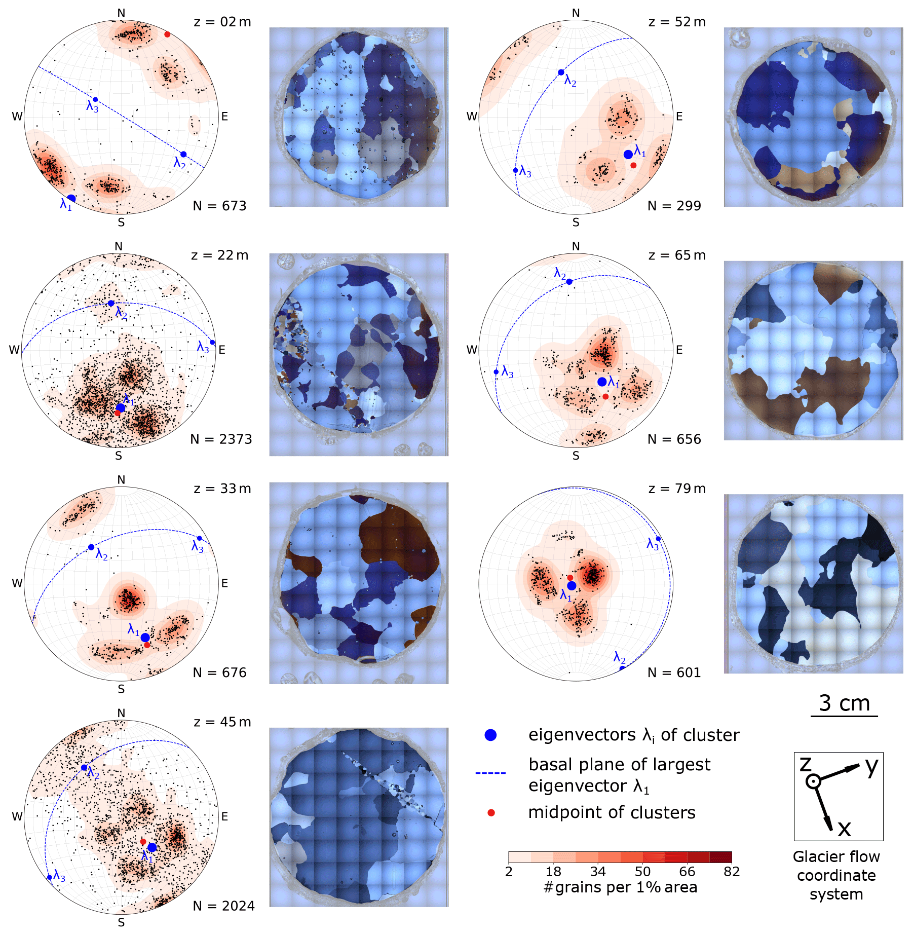
Figure 5Left columns: stereo-plots (lower-hemisphere Schmidt equal-area projection onto the horizontal, i.e. long axis of core plots in the centre) with the c-axis distribution and associated horizontal thin sections, illustrating the typical grain size distribution, shown for each sample. The total number of ice grains (N) is specified for each sample (consisting of at least three horizontal and six vertical thin sections, all rotated to a horizontal view and common geographic coordinates). The sampling depth (z) is indicated in the upper right corner of the stereo-plots. The colour code (smoothed Kamb's distribution; Vollmer, 1995) emphasises the existing clusters of the c-axis distribution. The eigenvectors for the determined distribution are depicted as blue dots, and the normal plane of the largest eigenvector is shown as a dashed line. Right columns: example images of horizontal thin sections, recorded under cross-polarised light; pale edges around the actual samples are excluded from analysis.
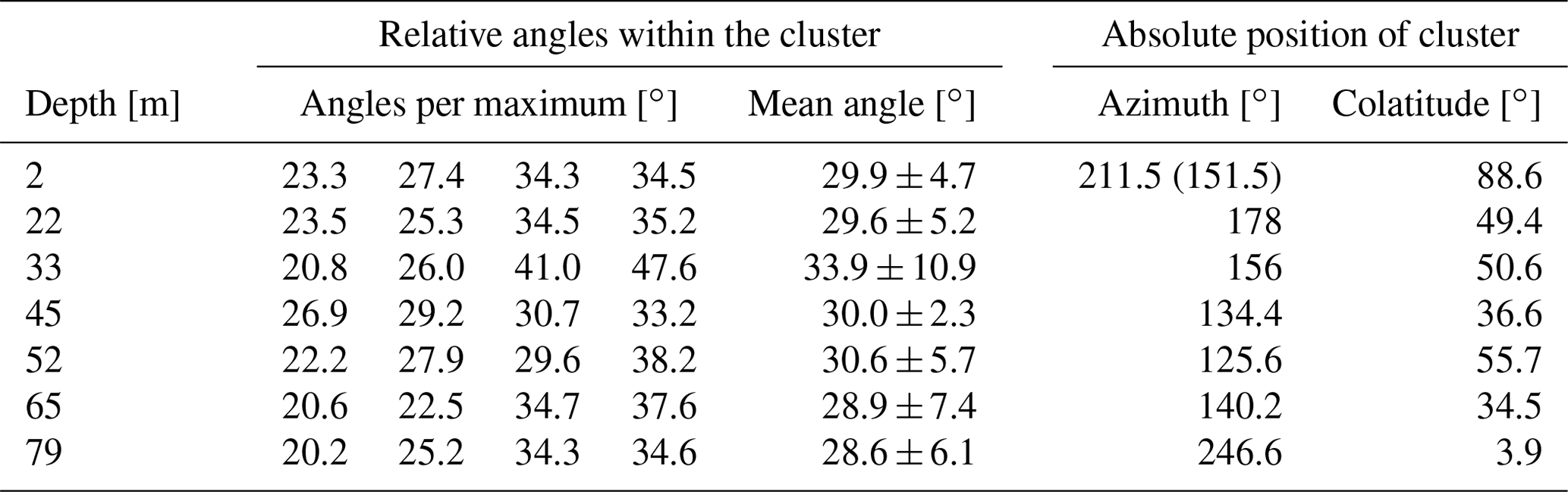
For better visualising of the c-axis distributions, a smoothed colour density plot, calculated in accordance with Kamb's method (Vollmer, 1995), was superimposed on the stereo-plots. These density plots only consider the number of grains within the area of the stereo-plot; i.e. the size of the individual grains does not affect the colour code. All density plots indicate a multi-maxima pattern, and the majority exhibits four maxima. The orientation of the patterns varies with depth, but the structure inside the patterns is remarkably similar. The four maxima lie on a small circle girdle, which is characterised by an opening angle around a central vector, shown as a midpoint in the stereographic projection. Two maxima always lie on opposite sides of this midpoint and the other two on a line perpendicular to the first two clusters so that the azimuthal separation of the maxima is 90∘. Deviations are observed at 45 m depth, where a fifth maximum at the horizontal margin appears, and at 79 m, where one of the four maxima is significantly weaker than the others. Depending on the number of grains per cluster, the midpoint (red point in Fig. 5) differs from the actual centroid (blue dot λ1 in Fig. 5) of the multi-maxima pattern. The opening angle between the midpoint and the individual maxima varies with ±15∘ around a mean of 30∘ (Table 1), but the mean value is constant over all depths.
The eigenvectors of the polycrystalline orientation tensor were calculated for each depth, and they are also shown in the stereo-plots (blue dots in Fig. 5). For enhanced visibility, the plane normal to the eigenvector associated with the largest eigenvalue λ1 is indicated with a dashed blue line. This eigenvector coincides with the centroid of the four-point maxima. The other two eigenvalues are significantly lower than λ1 (0.56 0.7) and usually in a range of 0.1 0.31 and 0.09 0.13, respectively.
With an exception for the uppermost depth at 2 m and the lowermost depth at 79 m, the azimuth of the maximum eigenvectors (147∘ ± 31∘) is aligned with the direction of the glacier's ice flow (155∘ ± 10∘; see Figs. 1, 2). With increasing depth, the maximum eigenvector has a decreasing colatitude, and at 79 m this eigenvector as well as the centroid of the cluster is almost vertically oriented.
Table 1Angles between individual maxima and the centroid, i.e. the largest eigenvector, describing the relative geometry of the multi-maxima pattern and the absolute orientation (azimuth and colatutide) of the centroid.
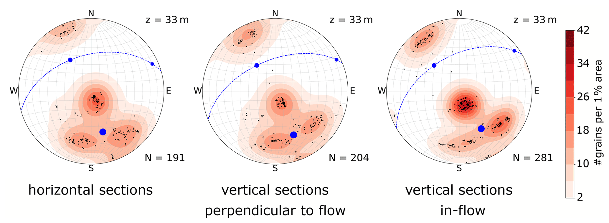
For an enhanced and statistically significant data set, we combined the determined c-axis orientations measured from up to 12 individual thin sections. These individual thin sections belong to one of the three different orientations (Fig. 4). However, the results from the different orientations of the sections may be inconsistent. Although the grains are not elongated in a certain direction (i.e. do not show a shape preferred orientation), some of them appear branched and interlocked (Fig. 5, right panels). Therefore, two-dimensional cuts through large, branched grains may let them appear as several individual grains within the same section. Kamb (1959) and Hooke (1969) have already discussed the statistical relevance of these branched grains. The sketches in Hooke and Hudleston (1980), their Fig. 6, and more recently in Monz et al. (2021), their Fig. 3, further illustrate this issue that could result in over-represented clusters in the superimposed stereo-plots from the different sub-samples.
To check the consistency of the individual orientations, the c-axis distribution for each sub-section (horizontal, east–west and south–north) was analysed separately. Figure 6 shows the results for the sample at 33 m depth. All three sub-sections show a similar pattern. The individual maxima appear in all sections and are not a result of stitching differently oriented sections together. However, due to the aforementioned reasons, the actual grain size is difficult to determine. Individual analyses for the other depths showed similarly consistent results (not shown).
For our interpretation, we refer to the deviatoric stress tensor elements. The absolute values are shown in Fig. 7 ( and ). The x component of the tensor elements is aligned with the longitudinal direction, i.e. the glacier flow, and the y component is aligned with the transverse direction. Due to the flow evolution of the ice grains through the glacier, these grains are deformed under given stress conditions (Schulson and Duval, 2009, chap. 5). As the glacier changes its flow direction, the ice crystals experience changing stress conditions leading to variations in the deformation regime. As a result, the c axes of the ice grains are oriented in specific patterns, such as the multi-maxima structure that we observed in the current ice core. The stress and strain rate are directly linked via Glen's flow law, and changing stress causes a change in deformation geometry. However, the particular orientation of ice grains is crucial as to whether the ice is easy to deform (“soft” direction) or whether it is further resistive (“hard” direction) to the currently applied deformation. For a detailed analysis of the current stress conditions at the ice core location, we use the ice flow model to derive the deviatoric stress tensor.
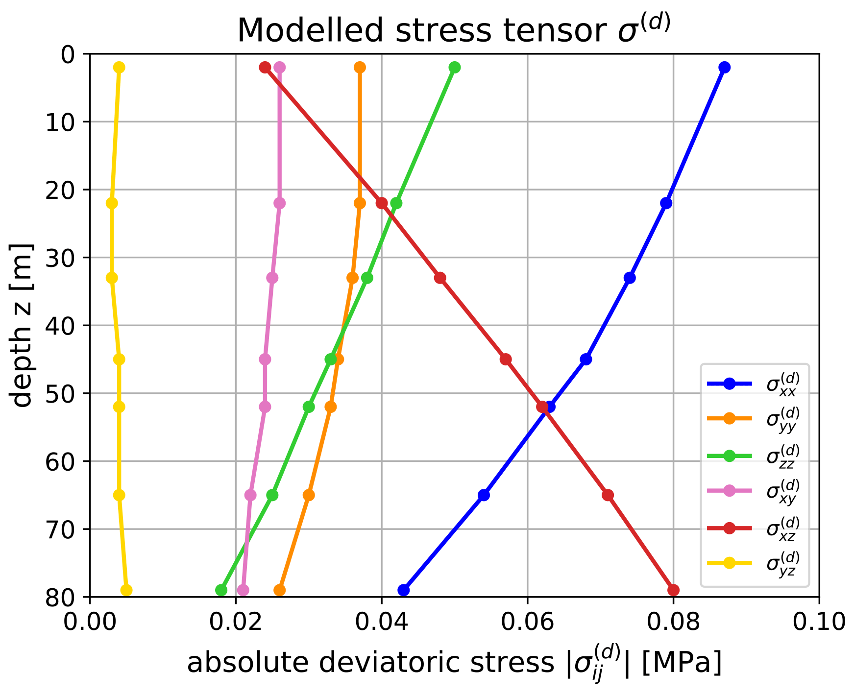
Figure 7Absolute values of the deviatoric stress tensor elements obtained from ice flow modelling (x – longitudinal, y – transverse, z – vertical direction).
The deviatoric stress tensor σ(d) is derived from the normal stress tensor σ by subtracting the isotropic pressure p from its main diagonal elements; i.e.
where δij=1 for i=j and δij=0 otherwise. For the deformation of the ice grains only the deviatoric stress tensor is important. The two most relevant components at the core location are the longitudinal compressional stress and the longitudinal shear stress (Fig. 7). is the most dominant stress close to the surface. Its strength slightly decreases with depth. In addition, the shear stress governs the stress conditions in deeper parts as it increases with depth. The transverse components (, and ) are more or less equal at all depths.
Table 2Strain rates derived from ice flow modelling (x – longitudinal, y – transverse, z – vertical direction).

We also calculate the strain rates from the stress tensor by using Glen's flow law, i.e. Eq. (1) (Table 2). Since the model does not consider anisotropy, the orientation-dependent response of the anisotropic ice is not considered. For typical fabrics (e.g. single-maximum, girdle), enhancement factors could be introduced (e.g. Thorsteinsson, 2001; Pettit et al., 2007; Ma et al., 2010) to overcome this issue. Beyond this, anisotropic flow laws (e.g. Gillet-Chaulet et al., 2005) can be employed to consider more complex fabrics such as the multi-maxima pattern. Furthermore, in isotropic models, the stress and strain rate are connected with a scalar value and the principal axes of stress and strain rate tensors are parallel. This is a crucial limitation to be considered in the following interpretation. Especially for shear stress, the model-derived and the actual strain rate directions may differ significantly. In addition, the quantitative numbers deviate from isotropic ice as the aforementioned basal sliding affects the strain rates that an ice grain experiences. However, we regard the modelling output as auxiliary values for our interpretation.
In the following, we provide an interpretation of three significant features presented in Fig. 5, namely
-
the azimuthal orientation of the c-axes distributions as represented by the maximum eigenvectors of the stress tensors,
-
the decrease in the maximum eigenvector colatitudes with increasing depths (viz. this eigenvector becomes more vertical), and
-
the existence of multi-maxima patterns in the c-axis distributions.
To support the interpretation, the stereo-plots in Fig. 5 are shown again in Fig. 8 with adjustments as a result of the following interpretation. Here, only the colour-coded c-axis density distributions are plotted, superimposed by additional information obtained from accompanying analyses.
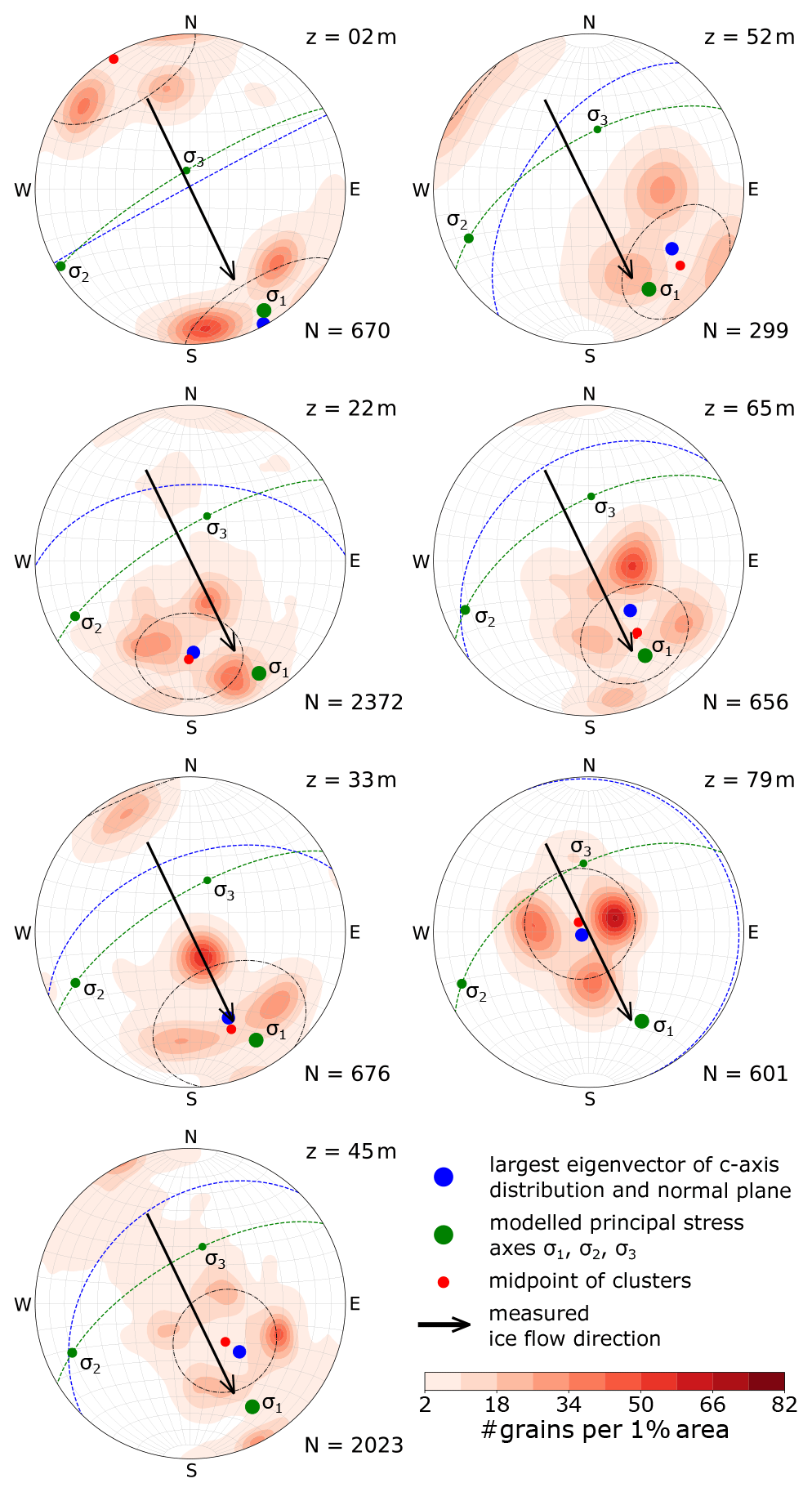
Figure 8Stereo-plots (lower-hemisphere Schmidt equal-area projection) with the colour-coded (same as Fig. 5) c-axis distribution for each sample shown. Note that the azimuth for z=2 m is corrected by −60∘ (see text for discussion). The total number of ice grains is specified for each sample. The dashed black line shows the mean opening angle for the cone of maxima around the centroid depicted as a red dot. The calculated largest eigenvector for the c-axis distribution is shown as a blue dot (its normal plane as a dashed blue line), and the calculated largest compressional principal stress axis from the ice flow model is represented by a green dot (its normal plane as a dashed green line).
6.1 Azimuthal orientation
Results from all depth levels, with the exception for 2 m (Fig. 5), show in general a mean c-axis orientation (Table 1) approximately parallel to the main glacier flow direction that was obtained from the displacements of the surrounding boreholes (Fig. 2; ≈ 155∘). The largest eigenvector λ1 always lies in a vertical plane that is aligned (±20∘) with the glacier flow direction. This flow kinematics, depicted by the principal stress axis (Figs. 5 and 8), are associated with the alignment of the centroid of the c axes. As this flow direction changes, the COF has most likely developed since the glacier flows in the direction observed at our drill location. Although the centroid at 79 m is vertically oriented, the characteristic “diamond shape” of the multi-maxima pattern is still joining the vertical plane of the glacier flow direction (the verticality of the pattern is discussed below).
The observed azimuthal alignment of the COF with the glacier flow (with some limitations for 79 m) is in accordance with results from laboratory experiments in a number of previous studies (e.g. Kamb, 1972; Duval, 1981; Budd and Jacka, 1989) and comparable with some parts of the Cape Folger ice core (Thwaites et al., 1984).
The uppermost sample (2 m) does not fit into this interpretation. Although the magnetometer data are consistent, the core break between two segments at 10 m was unclear and we cannot fully exclude a misorientation between the segments at 2 and 22 m. As shown in Fig. 8 an azimuthal correction of −60∘ would lead to a perfect alignment of this sample with all other observations and the modelling results for the particular location. Therefore, we assume a misorientation of the core segments.
6.2 Colatitude variations
In the following, we consider the variations in the colatitude of the largest eigenvector λ1 (Fig. 8, blue dot). There is a decrease in the colatitude from 89 to 4∘ with increasing depth (Table 1). Considering the deformation mechanisms, mainly dislocation creep, this is the result of the stress and strain rate distribution (Fig. 7 and Table 2) in the glacier. The ice crystal c axes in our samples generally orient themselves parallel to the ice flow, which coincides with the modelled maximum compressional principal stress direction (σ1 in Fig. 8). As indicated by the relative movements of the surrounding boreholes (Figs. 2 and 3), we indeed observe a compression at the glacier surface. In accordance with borehole inclination measurements, the flow-parallel compression also occurs at greater depths but slightly decreases. In contrast, with increasing depth, the shear stress significantly increases. Especially in the deepest parts of the ice core, the longitudinal shear component governs the stress state, which is also confirmed by the inclinometer measurements. This increasing shear deformation of the ice lets the colatitude angle decrease with increasing depths and explains, at least qualitatively, the observations in Fig. 8.
The principal stresses (σ1, σ2, σ3), derived from the ice flow model, were added to Fig. 8 (green dots) for comparison. Although not matching perfectly, the colatitudinal angles of the largest eigenvector λ1 and the dominant principal stress σ1 are similar within ±26∘ with an exception for the deepest sample. The discrepancy especially for the deepest sample is considered evidence that the c-axis distribution is governed by strain and not stress (Budd et al., 2013; Faria et al., 2014b; Weikusat et al., 2017). In the presence of simple shear, the direction of the principal stress axis and principal strain rate axis are not aligned (non-coaxial relation) Cuffey and Paterson (2010, chap. 3). This implies that the COF for the deepest sample is dominated by the shear component, which approaches simple shear. According to our strain rate components (Table 2), such an implication is justified. The modelled shear strain rate is twice as large as any other component and causes the most significant effect in the borehole measurements after a short time period.
6.3 Multi-maxima c-axis distribution
If the c-axis orientations were governed solely by the orientation of the major principal stress and strain rate direction (σ1) (mainly a result of compressional and simple shear stress), we would instead expect a single maximum in the stereo-plots as in deeper parts of other ice cores (Faria et al., 2014a). As observed in Figs. 5 and 8, there is no single maximum. Instead, the individual c axes in our samples deviate on average by about 30∘ from the principal stress or strain rate (for 79 m) direction (indicated by small black circles in Fig. 8) and group into several maxima.
The most likely reason for this observation involves recrystallisation processes. In general, two types of recrystallisation have been considered, namely rotation recrystallisation (RRX) and migration recrystallisation (Alley et al., 1995). RRX (described in detail in Alley, 1988) counteracts the dynamic grain growth (Weikusat et al., 2011b). According to Faria et al. (2014b), migration recrystallisation, also called strain-induced boundary migration (SIBM), needs to be subdivided into two types, namely SIBM-O and SIBM-N. In both cases, grains with fewer dislocations grow at the cost of grains with a large number of dislocations. The first type assumes that under given strain rate conditions, already existing (i.e. old), suitably oriented grains grow at the cost of less suitably oriented grains (called SIBM-O). The second type is very similar but with a relevant difference: when the grain grows, parts at the boundaries like bulges can be nuclei for new smaller grains (therefore called SIBM-N; see an exemplary process described by Steinbach et al., 2017, with a very similar orientation of new grains to their parent grain). These new grains are considered strain-free grains and have an impact on the grain size. Both mechanisms are driven by reducing the thermodynamic energy of the whole system and grains with heterogeneously distributed dislocations are absorbed (Weikusat et al., 2009b, their Fig. 8).
Table 3Grain size distribution (median, mean and maximum grain sizes [mm2]; minimum grain size is 0.2 mm2 and defined as the threshold during processing) and number of grains within defined grain size classes [mm2].
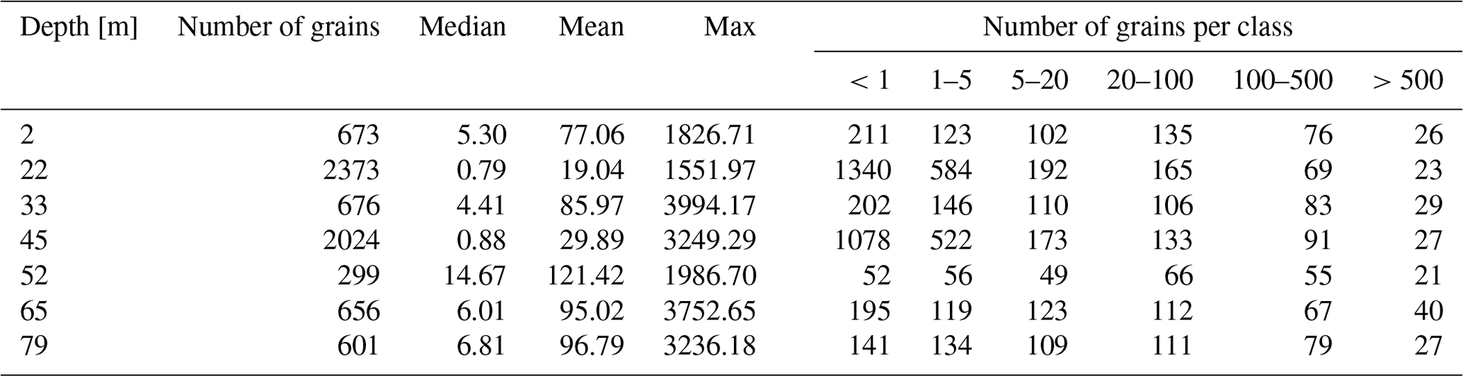
In our data set we observe a variety of different grain sizes. Table 3 summarises the grain size distribution in our ice core samples. As mentioned earlier, the two-dimensional cuts through the ice core samples may lead to a misinterpretation of the grain sizes as large interlocked grains can appear as several small grains. However, it can be expected that not all small grains are cut branches of large grains. We also analysed the COF for six different grain size classes individually. The data are shown in Fig. 9 for one sample (other samples in the Appendix A). The multi-maxima pattern is persistent in all grain size classes. Based on these findings, we postulate that this pattern is a result of SIBM-N in combination with the described longitudinal compressional and shear stress.
However, our data set cannot conclusively explain the very regular distribution of c axes, i.e. the diamond shape, within the multi-maxima pattern.

Figure 9Stereo-plots (lower-hemisphere Schmidt equal-area projection) with the colour coding the same as in Fig. 5. Each plot represents a grain size class as indicated in the upper right corner. The number of grains per class is specified for each plot. The calculated eigenvectors for the c-axis distribution are shown as blue dots (the normal plane for the largest eigenvector is shown as a dashed blue line). Right column: histogram showing the number of grains per class.
The literature on COF field studies is not conclusive concerning the existence of multi-maxima fabrics. They were observed in early studies on temperate glaciers (e.g. Rigsby, 1951; Kamb, 1959; Rigsby, 1960) for the first time. In the 1970s to 1980s, they were found in ice caps with ice temperatures above −10 ∘C (Hooke and Hudleston, 1980) and also in the bottom ice of Byrd Station and Cape Folger in Antarctica (Gow and Williamson, 1976; Thwaites et al., 1984). At that time, the estimation of c-axis distributions was more subjective and could not benefit from modern equipment. The orientation of crystals was determined manually on a Rigsby stage by turning and tilting the ice samples between polarised plates. Thus, only a limited number of grains (up to 100) and usually the largest grains were analysed. Therefore, it was often debated whether the diamond shape pattern was a statistical effect.
Interestingly, in more recent studies on other temperate glaciers, multi-maxima fabrics in combination with a large grain size were only observed in the deepest parts of the ice cores drilled in the ablation zone (e.g. Tison and Hubbard, 2000). The conditions for a diamond shape pattern seem to be suitable in large glaciers like Rhonegletscher with its high temperatures and large ice flow velocities compared to other valley glaciers. In polar ice cores, a multi-maxima fabric has been observed only in the deepest parts of some Antarctic and Greenlandic cores (Gow and Williamson, 1976; Thwaites et al., 1984; Montagnat et al., 2014). There, the temperature conditions are as high as in temperate glaciers like Rhonegletscher.
Laboratory experiments, performed on artificial ice under high temperatures ( ∘C), provide evidence for two features we observe. Maohuan et al. (1985) created multi-maxima fabrics with combined shear and compressional stresses in their torsion–compression experiments. The pattern clustered around the maximum principal stress direction. In addition, Jacka and Maccagnan (1984) analysed the opening angle of small circle girdles formed under compressional stress. The ranges for the opening angles are identical with our observations. For such opening angles between compressional direction and the c-axis direction, the compressive strength applied onto the ice crystal is minimised (Schulson and Duval, 2009, chap. 11).
As a result of these laboratory experiments and field measurements, we conclude that these temperate conditions in Rhonegletscher are a prerequisite for the development of multi-maxima patterns, but a multi-maxima pattern is not necessarily found in all temperate glaciers.
Recrystallisation has regularly been observed in a variety of ice cores (Alley, 1988; Duval and Castelnau, 1995; Weikusat et al., 2009b; Schulson and Duval, 2009; Cuffey and Paterson, 2010; Faria et al., 2014b). Recrystallisation has usually been divided into two types – rotation and migration recrystallisation. However, according to Faria et al. (2014b), migration recrystallisation, also called strain-induced boundary migration (SIBM), needs to be subdivided into two types (SIBM-O and SIBM-N). These two mechanisms lead to different COFs. If SIBM-O is the dominating process, a single maximum consisting of a few very large grains is expected to develop. For SIBM-N we regularly generate new grains with a similar orientation to the parent grain and concurrent maxima are likely to develop. This can lead to the observed multi-maxima fabric. Evidence for a dominating grain boundary migration with nucleation (SIBM-N) can be observed in LASM scans (Fig. 10). Firstly, the air bubbles are trapped within grains with a diameter of centimetres. Secondly, the grain boundaries of neighbouring grains bulge and smaller grains develop either as “island grains” or as clusters along the boundaries of the large grains (blue, red and yellow circles in Fig. 10). The trapped air bubbles and newly developing grains provide evidence that SIBM-N is the dominating process in these samples of temperate ice.
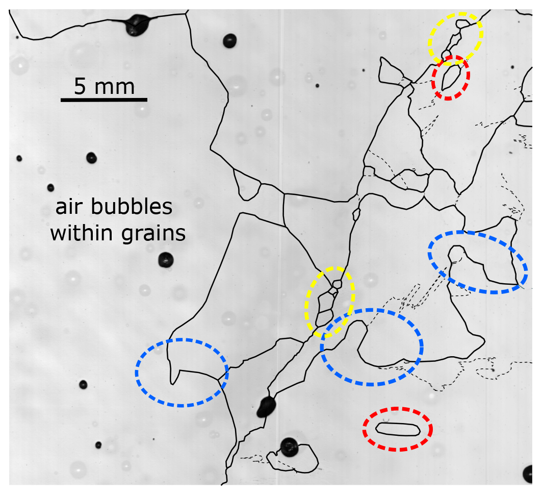
Figure 10Example of a LASM image indicating several processes in the temperate ice: black areas are air bubbles; black lines represent the grain boundaries; and dashed black lines indicate subgrain boundaries. Air bubbles can be found completely trapped within individual large ice grains, indicating migration recrystallisation. Bulging of grain boundaries (blue circles), the development of island grains (red circles) and small grains along the boundaries of large grains (yellow circles) provide evidence for a dominating SIBM-N-type recrystallisation.
The recrystallisation does not conclusively provide arguments for the regular diamond shape within the multi-maxima pattern. One potential mechanism to be considered comprises localisation effects. In this theory, the polycrystalline system distributes the impact of the different strain along localisation bands, especially in the presence of additional aggregates such as air bubbles (Steinbach et al., 2016). This may lead to a highly variable rate of fabric change. A detailed investigation of localisation bands is rather difficult in the presence of grain boundary migration (i.e. SIBM-O and SIBM-N) as recrystallisation restores the crystal shape and removes the typical shear bands (Llorens et al., 2016). Llorens et al. (2017) investigated the COF for simple shear experiments by considering localisation bands and dynamic recrystallisation (rotational recrystallisation and grain boundary migration but without nucleation). These strain-induced localisation effects might be worth considering for explaining multi-maxima patterns.
Further alternative explanations can and should be considered: Kamb (1959) calculated the preferred maximum positions of a diamond shape pattern with considerations of single crystal compliance constants under recrystallisation. This explanation could add missing details to our interpretation and describe the regularity in the diamond shape pattern. Matsuda and Wakahama (1978) suggest twinning effects that may occur when c axes develop under recrystallisation. Potentially, these effects may lead to a clustering of the c axes and would even better explain the regular shape of the COF. This theory is supported by the fact that the opening angles of two opposing clusters are generally similar, whereas the angles compared to the other two maxima can vary within 15–20∘ and are therefore called diamond shape fabrics. Apart from that, it is hard to find any studies about observations on twinning as result of ice deformation in glaciers, and Faria et al. (2014b) summarised that mechanical twinning has not been observed in glacier ice. To investigate this further, we would need to measure the orientation of the ice crystals' a axes (in addition to the c axes), for an enhanced image about the crystal orientation in three dimensions (Weikusat et al., 2011a; Journaux et al., 2019; Monz et al., 2021).
COF analyses of an ice core, extracted from a temperate alpine glacier, showed conspicuous multi-maxima patterns of the c axes. This was observed at different depth levels. The azimuth and colatitude of the centroid of these multi-maxima patterns are well-aligned with the main principal stress direction. Close to the surface, compressional longitudinal stress conditions lead to a horizontal orientation aligned with the glacier flow. In deeper parts, the dominating longitudinal shear stress causes a vertical COF. The mean basal plane is aligned with the shear plane.
Strain-induced boundary migration with nucleation of new grains (SIBM-N) seems to be the dominating recrystallisation process under the given high temperatures and strain rates. This provides an explanation for the large and branched grains accompanied by smaller grains with similar orientation and thus a clustering in several maxima. However, the observations cannot conclusively provide an explanation for the very regular diamond shape pattern.
To the best of our knowledge, this is the first comprehensive COF analysis of an ice core from a temperate alpine glacier that links the COF with the glacier flow. The results are consistent with supporting measurements and modelling results. These consistencies are encouraging and will hopefully motivate similar studies on other temperate glaciers.

Figure A1Stereo-plots (lower-hemisphere Schmidt equal-area projection) with the colour coding the same as in Fig. 5. Each column represents a grain size class as indicated at the top. Each line represents one of the seven samples of Fig. 5. The number of grains per class is specified for each plot. The largest calculated eigenvector for the c-axis distribution is shown as a blue dot (its normal plane as a dashed blue line). Last column: histograms showing the number of grains per class for each sample.
The ice fabric data and the LASM images are published in the open-access database PANGAEA® (https://doi.org/10.1594/PANGAEA.888518 – Hellmann et al., 2018a; https://doi.org/10.1594/PANGAEA.888517 – Hellmann et al., 2018b).
This study was initiated and supervised by HM, AB, IW and MS. The field and laboratory data were collected by MS, SH, MG, AB and JK and analysed by SH with support from JK and under supervision of IW and MS. Data processing and calculations were made and interpreted by SH and discussed with JK, IW and MG. The ice flow was modelled by GJ with input data from MG. The paper was written by SH with comments and suggestions for improvements from all co-authors.
The authors declare that they have no conflict of interest.
This project is funded by the Swiss National Science Foundation under the SNF grants 200021_169329/1 and 200021_169329/2. Data acquisition has been provided by the Paul Scherrer Institute, Villingen; the Alfred Wegener Institute Helmholtz Centre for Polar and Marine Research (AWI), Bremerhaven; and the Laboratory of Hydraulics, Hydrology and Glaciology (VAW) of ETH Zurich. We especially thank Jan Eichler, Tamara Gerber, Theo Jenk and Dieter Stampfli for their extensive technical and logistical support during ice core drilling and processing. Valuable discussions with the Structural Glaciology group at the University of Tübingen helped to improve the paper. We would like to thank the editor, Olivier Gagliardini, and the two reviewers, Erin Pettit and Peter Hudleston, for their constructive comments, which greatly improved the quality of the manuscript.
This research has been supported by the Swiss National Science Foundation (grant no. 200021_169329/1 and 200021_169329/2).
This paper was edited by Olivier Gagliardini and reviewed by Peter Hudleston and Erin Pettit.
Alley, R. B.: Fabrics in Polar Ice Sheets: Development and Prediction, Science, 240, 493–495, 1988. a, b, c, d
Alley, R. B.: Flow-Law Hypotheses for Ice-Sheet Modeling, J. Glaciol., 38, 245–256, 1992. a
Alley, R. B., Gow, A. J., and Meese, D. A.: Mapping C-Axis Fabrics to Study Physical Processes in Ice, J. Glaciol., 41, 197–203, 1995. a, b
Alley, R. B., Gow, A. J., Meese, D. A., Fitzpatrick, J. J., Waddington, E. D., and Bolzan, J. F.: Grain-Scale Processes, Folding, and Stratigraphic Disturbance in the GISP2 Ice Core, J. Geophys. Res.-Oceans, 102, 26819–26830, https://doi.org/10.1029/96JC03836, 1997. a
Azuma, N.: A Flow Law for Anisotropic Ice and Its Application to Ice Sheets, Earth Planet. Sci. Lett., 128, 601–614, https://doi.org/10.1016/0012-821X(94)90173-2, 1994. a
Azuma, N., Miyakoshi, T., Yokoyama, S., and Takata, M.: Impeding Effect of Air Bubbles on Normal Grain Growth of Ice, J. Struct. Geol., 42, 184–193, https://doi.org/10.1016/j.jsg.2012.05.005, 2012. a
Bauder, A.: The Swiss Glaciers 2015/16 and 2016/17, Cryospheric Commission (EKK) of the Swiss Academy of Sciences (SCNAT), Glaciological Report, 137/138, 145 pp., https://doi.org/10.18752/glrep_137-138, 2018. a
Binder, T., Garbe, C. S., Wagenbach, D., Freitag, J., and Kipfstuhl, S.: Extraction and Parametrization of Grain Boundary Networks in Glacier Ice, Using a Dedicated Method of Automatic Image Analysis, J. Microsc., 250, 130–141, https://doi.org/10.1111/jmi.12029, 2013. a
Budd, W. F.: The Development of Crystal Orientation Fabrics in Moving Ice, Z. Gletscherkd. Glazialgeol., 8, 65–105, 1972. a
Budd, W. F. and Jacka, T. H.: A Review of Ice Rheology for Ice Sheet Modelling, Cold Reg. Sci. Technol., 16, 107–144, https://doi.org/10.1016/0165-232X(89)90014-1, 1989. a, b
Budd, W. F., Warner, R. C., Jacka, T. H., Li, J., and Treverrow, A.: Ice Flow Relations for Stress and Strain-Rate Components from Combined Shear and Compression Laboratory Experiments, J. Glaciol., 59, 374–392, https://doi.org/10.3189/2013JoG12J106, 2013. a
Church, G. J., Bauder, A., Grab, M., Hellmann, S., and Maurer, H.: High-Resolution Helicopter-Borne Ground Penetrating Radar Survey to Determine Glacier Base Topography and the Outlook of a Proglacial Lake, in: Proceedings of the 17th International Conference on Ground Penetrating Radar (GPR), 18–21 June 2018, Rapperswil, Switzerland, 1–4, https://doi.org/10.1109/ICGPR.2018.8441598, 2018. a, b
Compagno, L., Jouvet, G., Bauder, A., Funk, M., Church, G., Leinss, S., and Lüthi, M. P.: Modeling the Re-Appearance of a Crashed Airplane on Gauligletscher, Switzerland, Front. Earth Sci., 7, 170, https://doi.org/10.3389/feart.2019.00170, 2019. a
Cuffey, K. M. and Paterson, W. S. B.: The Physics of Glaciers, Elsevier, Amsterdam, 2010. a, b, c, d
Diez, A. and Eisen, O.: Seismic wave propagation in anisotropic ice – Part 1: Elasticity tensor and derived quantities from ice-core properties, The Cryosphere, 9, 367–384, https://doi.org/10.5194/tc-9-367-2015, 2015. a
Duval, P.: Creep and Recrystallization of Polycrystalline Ice, B. Mineral., 102, 80–85, https://doi.org/10.3406/bulmi.1979.7258, 1979. a
Duval, P.: Creep and Fabrics of Polycrystalline Ice Under Shear and Compression, J. Glaciol., 27, 129–140, https://doi.org/10.3189/S002214300001128X, 1981. a
Duval, P. and Castelnau, O.: Dynamic Recrystallization of Ice in Polar Ice Sheets, J. Phys. IV, 5, 3–197, 1995. a
Eichler, J.: C-Axis Analysis of the NEEM Ice Core – An Approach Based on Digital Image Processing, Diploma Thesis, Freie Universität Berlin, Berlin, Germany, 73 pp., 2013. a, b
Faria, S. H., Freitag, J., and Kipfstuhl, S.: Polar Ice Structure and the Integrity of Ice-Core Paleoclimate Records, Quaternary Sci. Rev., 29, 338–351, https://doi.org/10.1016/j.quascirev.2009.10.016, 2010. a
Faria, S. H., Weikusat, I., and Azuma, N.: The Microstructure of Polar Ice. Part I: Highlights from Ice Core Research, J. Struct. Geol., 61, 2–20, https://doi.org/10.1016/j.jsg.2013.09.010, 2014a. a, b, c
Faria, S. H., Weikusat, I., and Azuma, N.: The Microstructure of Polar Ice. Part II: State of the Art, J. Struct. Geol., 61, 21–49, https://doi.org/10.1016/j.jsg.2013.11.003, 2014b. a, b, c, d, e, f
Farinotti, D., Huss, M., Bauder, A., Funk, M., and Truffer, M.: A Method to Estimate the Ice Volume and Ice-Thickness Distribution of Alpine Glaciers, J. Glaciol., 55, 422–430, 2009. a
Gagliardini, O., Zwinger, T., Gillet-Chaulet, F., Durand, G., Favier, L., de Fleurian, B., Greve, R., Malinen, M., Martín, C., Råback, P., Ruokolainen, J., Sacchettini, M., Schäfer, M., Seddik, H., and Thies, J.: Capabilities and performance of Elmer/Ice, a new-generation ice sheet model, Geosci. Model Dev., 6, 1299–1318, https://doi.org/10.5194/gmd-6-1299-2013, 2013. a
Gillet-Chaulet, F., Gagliardini, O., Meyssonnier, J., Montagnat, M., and Castelnau, O.: A User-Friendly Anisotropic Flow Law for Ice-Sheet Modeling, J. Glaciol., 51, 3–14, https://doi.org/10.3189/172756505781829584, 2005. a
Glen, J. W.: The Creep of Polycrystalline Ice, Proc. Roy. Soc. Lond. A, 228, 519–538, https://doi.org/10.1098/rspa.1955.0066, 1955. a
Gow, A. J. and Meese, D.: Physical Properties, Crystalline Textures and c-Axis Fabrics of the Siple Dome (Antarctica) Ice Core, J. Glaciol., 53, 573–584, https://doi.org/10.3189/002214307784409252, 2007. a
Gow, A. J. and Williamson, T.: Rheological Implications of the Internal Structure and Crystal Fabrics of the West Antarctic Ice Sheet as Revealed by Deep Core Drilling at Byrd Station, Geol. Soc. Am. Bull., 87, 1665–1677, 1976. a, b, c, d, e
Grab, M., Bauder, A., Ammann, F., Langhammer, L., Hellmann, S., Church, G. J., Schmid, L., Rabenstein, L., and Maurer, H. R.: Ice volume estimates of Swiss glaciers using helicopter-borne GPR – an example from the Glacier de la Plaine Morte, in 2018 17th International Conference on Ground Penetrating Radar (GPR), 18–21 June 2018, Rapperswil, 1–4, https://doi.org/10.1109/ICGPR.2018.8441613, 2018. a
Gräff, D., Walter, F., and Bauder, A.: orehole Measurements and Basal Velocity of Rhonegletscher: Analysis of Borehole Measurements and Determination of the Basal Sliding Velocity of Rhonegletscher, 15th Swiss Geoscience Meeting (SGM 2017, 17–18 November), Davos, 9–10, https://doi.org/10.3929/ethz-b-000444720, 2017. a
Hambrey, M. J. and Milnes, A. G.: Structural Geology of an Alpine Glacier (Griesgletscher, Valais, Switzerland), Eclogae Geol. Helv., 70, 667–684, 1977. a, b, c
Hambrey, M. J., Milnes, A. G., and Siegenthaler, H.: Dynamics and Structure of Griesgletscher, Switzerland, J. Glaciol., 25, 215–228, https://doi.org/10.3189/S0022143000010455, 1980. a
Hellmann, S., Kerch, J., Eichler, J., Jansen, D., Weikusat, I., Schwikowski, M., Bauder, A., and Maurer, H.: Crystal C-Axes Measurements (Fabric Analyser G50) of Ice Core Samples Collected from the Temperate Alpine Ice Core Rhone_2017, PANGAEA, https://doi.org/10.1594/PANGAEA.888518, 2018a. a
Hellmann, S., Kerch, J., Eichler, J., Jansen, D., Weikusat, I., Schwikowski, M., Bauder, A., and Maurer, H.: Large Area Scan Macroscope Images of Ice Core Samples Collected from the Temperate Alpine Ice Core Rhone_2017, PANGAEA, https://doi.org/10.1594/PANGAEA.888517, 2018b. a
Herron, S. L. and Langway, C. C.: A Comparison of Ice Fabrics and Textures at Camp Century, Greenland and Byrd Station, Antarctica, Ann. Glaciol., 3, 118–124, 1982. a
Hooke, R. L.: Crystal Shape in Polar Glaciers and the Philosophy of Ice-Fabric Diagrams, J. Glaciol., 8, 324–326, https://doi.org/10.3189/S002214300003135X, 1969. a
Hooke, R. L.: Structure and Flow in the Margin of the Barnes Ice Cap, Baffin Island, N.W.T., Canada, J. Glaciol., 12, 423–438, https://doi.org/10.3189/S0022143000031841, 1973. a
Hooke, R. L. and Hudleston, P. J.: Origin of Foliation in Glaciers, J. Glaciol., 20, 285–299, https://doi.org/10.3189/S0022143000013848, 1978. a
Hooke, R. L. and Hudleston, P. J.: Ice Fabrics in a Vertical Flow Plane, Barnes Ice Cap, Canada, J. Glaciol., 25, 195–214, https://doi.org/10.3189/S0022143000010443, 1980. a, b
Jacka, T. H. and Maccagnan, M.: Ice Crystallographic and Strain Rate Changes with Strain in Compression and Extension, Cold Reg. Sci. Technol., 8, 269–286, https://doi.org/10.1016/0165-232X(84)90058-2, 1984. a
Jansen, D., Llorens, M.-G., Westhoff, J., Steinbach, F., Kipfstuhl, S., Bons, P. D., Griera, A., and Weikusat, I.: Small-scale disturbances in the stratigraphy of the NEEM ice core: observations and numerical model simulations, The Cryosphere, 10, 359–370, https://doi.org/10.5194/tc-10-359-2016, 2016. a
Journaux, B., Chauve, T., Montagnat, M., Tommasi, A., Barou, F., Mainprice, D., and Gest, L.: Recrystallization processes, microstructure and crystallographic preferred orientation evolution in polycrystalline ice during high-temperature simple shear, The Cryosphere, 13, 1495–1511, https://doi.org/10.5194/tc-13-1495-2019, 2019. a
Jouvet, G. and Funk, M.: Modelling the Trajectory of the Corpses of Mountaineers Who Disappeared in 1926 on Aletschgletscher, Switzerland, J. Glaciol., 60, 255–261, https://doi.org/10.3189/2014JoG13J156, 2014. a
Jouvet, G., Huss, M., Blatter, H., Picasso, M., and Rappaz, J.: Numerical Simulation of Rhonegletscher from 1874 to 2100, J. Comput. Phys., 228, 6426–6439, https://doi.org/10.1016/j.jcp.2009.05.033, 2009. a
Jouvet, G., Huss, M., Funk, M., and Blatter, H.: Modelling the Retreat of Grosser Aletschgletscher, Switzerland, in a Changing Climate, J. Glaciol., 57, 1033–1045, https://doi.org/10.3189/002214311798843359, 2011. a
Kamb, B.: Experimental Recrystallization of Ice under Stress, American Geophysical Union Geophysical Monograph Series, Washington DC, USA, https://doi.org/10.1029/GM016p0211, 1972. a, b
Kamb, W. B.: Ice Petrofabric Observations from Blue Glacier, Washington, in Relation to Theory and Experiment, J. Geophys. Res., 64, 1891–1909, https://doi.org/10.1029/JZ064i011p01891, 1959. a, b, c, d, e
Krischke, A., Oechsner, U., and Kipfstuhl, S.: Rapid Microstructure Analysis of Polar Ice Cores, Optik Photonik, 10, 32–35, https://doi.org/10.1002/opph.201500016, 2015. a
Kuiper, E.-J. N., de Bresser, J. H. P., Drury, M. R., Eichler, J., Pennock, G. M., and Weikusat, I.: Using a composite flow law to model deformation in the NEEM deep ice core, Greenland – Part 2: The role of grain size and premelting on ice deformation at high homologous temperature, The Cryosphere, 14, 2449–2467, https://doi.org/10.5194/tc-14-2449-2020, 2020. a
Llorens, M.-G., Griera, A., Bons, P. D., Lebensohn, R. A., Evans, L. A., Jansen, D., and Weikusat, I.: Full-Field Predictions of Ice Dynamic Recrystallisation under Simple Shear Conditions, Earth Planet. Sc. Lett., 450, 233–242, https://doi.org/10.1016/j.epsl.2016.06.045, 2016. a
Llorens, M.-G., Griera, A., Steinbach, F., Bons, P. D., Gomez-Rivas, E., Jansen, D., Roessiger, J., Lebensohn, R. A., and Weikusat, I.: Dynamic Recrystallization during Deformation of Polycrystalline Ice: Insights from Numerical Simulations, Philos. T. R. Soc. A, 375, 20150346, https://doi.org/10.1098/rsta.2015.0346, 2017. a
Ma, Y., Gagliardini, O., Ritz, C., Gillet-Chaulet, F., Durand, G., and Montagnat, M.: Enhancement Factors for Grounded Ice and Ice Shelves Inferred from an Anisotropic Ice-Flow Model, J. Glaciol., 56, 805–812, https://doi.org/10.3189/002214310794457209, 2010. a
Maohuan, H., Ohtomo, M., and Wakahama, G.: Transition in Preferred Orientation of Polycrystalline Ice from Repeated Recrystallization, Ann. Glaciol., 6, 263–264, https://doi.org/10.3189/1985AoG6-1-263-264, 1985. a
Matsuda, M. and Wakahama, G.: Crystallographic Structure of Polycrystalline Ice, J. Glaciol., 21, 607–620, https://doi.org/10.3189/S0022143000033724, 1978. a
Montagnat, M., Azuma, N., Dahl-Jensen, D., Eichler, J., Fujita, S., Gillet-Chaulet, F., Kipfstuhl, S., Samyn, D., Svensson, A., and Weikusat, I.: Fabric along the NEEM ice core, Greenland, and its comparison with GRIP and NGRIP ice cores, The Cryosphere, 8, 1129–1138, https://doi.org/10.5194/tc-8-1129-2014, 2014. a, b
Monz, M. E., Hudleston, P. J., Prior, D. J., Michels, Z., Fan, S., Negrini, M., Langhorne, P. J., and Qi, C.: Full crystallographic orientation (c and a axes) of warm, coarse-grained ice in a shear-dominated setting: a case study, Storglaciären, Sweden, The Cryosphere, 15, 303–324, https://doi.org/10.5194/tc-15-303-2021, 2021. a, b
Morgenthaler, J.: Modelling the Spatial Distribution of the Age of Ice on Rhonegletscher, Switzerland, PhD thesis, ETH Zürich, Zurich, Switzerland, 71 pp., 2019. a
Patrick, B. A., Corvino, A. F., and Wilson, C. J. L.: Ice-Flow Measurements and Deformation at Marginal Shear Zones on Sørsdal Glacier, Ingrid Christensen Coast, East Antarctica, Ann. Glaciol., 37, 60–68, https://doi.org/10.3189/172756403781815933, 2003. a
Peternell, M., Kohlmann, F., Wilson, C. J., Seiler, C., and Gleadow, A. J.: A New Approach to Crystallographic Orientation Measurement for Apatite Fission Track Analysis: Effects of Crystal Morphology and Implications for Automation, Chem. Geol., 265, 527–539, https://doi.org/10.1016/j.chemgeo.2009.05.021, 2009. a, b
Petit, J. R., Jouzel, J., Raynaud, D., Barkov, N. I., Barnola, J.-M., Basile, I., Bender, M., Chappellaz, J., Davis, M., Delaygue, G., Delmotte, M., Kotlyakov, V. M., Legrand, M., Lipenkov, V. Y., Lorius, C., PÉpin, L., Ritz, C., Saltzman, E., and Stievenard, M.: Climate and Atmospheric History of the Past 420,000 Years from the Vostok Ice Core, Antarctica, Nature, 399, 429–436, https://doi.org/10.1038/20859, 1999. a
Pettit, E. C., Thorsteinsson, T., Jacobson, H. P., and Waddington, E. D.: The Role of Crystal Fabric in Flow near an Ice Divide, J. Glaciol., 53, 277–288, https://doi.org/10.3189/172756507782202766, 2007. a, b
Pettit, E. C., Waddington, E. D., Harrison, W. D., Thorsteinsson, T., Elsberg, D., Morack, J., and Zumberge, M. A.: The Crossover Stress, Anisotropy and the Ice Flow Law at Siple Dome, West Antarctica, J. Glaciol., 57, 39–52, https://doi.org/10.3189/002214311795306619, 2011. a
Rigsby, G. P.: Crystal Fabric Studies on Emmons Glacier Mount Rainier, Washington, J. Geol., 59, 590–598, 1951. a
Rigsby, G. P.: Crystal Orientation in Glacier and in Experimentally Deformed Ice, J. Glaciol., 3, 589–606, 1960. a, b, c, d
Robin, G. D. Q., Mitchell, G. F., and West, R. G.: Ice Cores and Climatic Change, Philos. T. R. Soc. B, 280, 143–168, https://doi.org/10.1098/rstb.1977.0103, 1977. a
Russell-Head, D. S. and Budd, W. F.: Ice-Sheet Flow Properties Derived from Bore-Hole Shear Measurements Combined With Ice-Core Studies, J. Glaciol., 24, 117–130, https://doi.org/10.3189/S0022143000014684, 1979. a
Schulson, E. M. and Duval, P.: Creep and fracture of ice, Cambridge University Press, Cambridge, UK, 2009. a, b, c, d
Schwikowski, M., Jenk, T. M., Stampfli, D., and Stampfli, F.: A New Thermal Drilling System for High-Altitude or Temperate Glaciers, Ann. Glaciol., 55, 131–136, https://doi.org/10.3189/2014AoG68A024, 2014. a
Steinbach, F., Bons, P. D., Griera, A., Jansen, D., Llorens, M.-G., Roessiger, J., and Weikusat, I.: Strain localization and dynamic recrystallization in the ice–air aggregate: a numerical study, The Cryosphere, 10, 3071–3089, https://doi.org/10.5194/tc-10-3071-2016, 2016. a
Steinbach, F., Kuiper, E.-J. N., Eichler, J., Bons, P. D., Drury, M. R., Griera, A., Pennock, G. M., and Weikusat, I.: The Relevance of Grain Dissection for Grain Size Reduction in Polar Ice: Insights from Numerical Models and Ice Core Microstructure Analysis, Front. Earth Sci., 5, 66, https://doi.org/10.3389/feart.2017.00066, 2017. a
Thompson, L. G., Mosley-Thompson, E., Davis, M. E., Henderson, K. A., Brecher, H. H., Zagorodnov, V. S., Mashiotta, T. A., Lin, P.-N., Mikhalenko, V. N., Hardy, D. R., and Beer, J.: Kilimanjaro Ice Core Records: Evidence of Holocene Climate Change in Tropical Africa, Science, 298, 589–593, https://doi.org/10.1126/science.1073198, 2002. a
Thorsteinsson, T.: An Analytical Approach to Deformation of Anisotropic Ice-Crystal Aggregates, J. Glaciol., 47, 507–516, https://doi.org/10.3189/172756501781832124, 2001. a
Thorsteinsson, T., Kipfstuhl, J., and Miller, H.: Textures and Fabrics in the GRIP Ice Core, J. Geophys. Res.-Oceans, 102, 26583–26599, https://doi.org/10.1029/97JC00161, 1997. a
Thwaites, R. J., Wilson, C. J. L., and McCray, A. P.: Relationship Between Bore-Hole Closure and Crystal Fabrics in Antarctic Ice Core from Cape Folger, J. Glaciol., 30, 171–179, https://doi.org/10.3189/S0022143000005906, 1984. a, b, c, d
Tison, J.-L. and Hubbard, B.: Ice Crystallographic Evolution at a Temperate Glacier: Glacier de Tsanfleuron, Switzerland, Geol. Soc. SP., 176, 23–38, 2000. a, b
Vollmer, F. W.: C Program for Automatic Contouring of Spherical Orientation Data Using a Modified Kamb Method, Comput. Geosci., 21, 31–49, 1995. a, b
Wallbrecher, E.: Tektonische Und Gefügeanalytische Arbeitsweisen: Graphische, Rechnerische Und Statistische Verfahren, Enke, Stuttgart, Germany, 1986. a
Weikusat, I., Kipfstuhl, S., Azuma, N., Faria, S. H., and Miyamoto, A.: Deformation Microstructures in an Antarctic Ice Core (EDML) and in Experimentally Deformed Artificial Ice, Low Temperature Science, 68, 115–123, 2009a. a
Weikusat, I., Kipfstuhl, S., Faria, S. H., Azuma, N., and Miyamoto, A.: Subgrain Boundaries and Related Microstructural Features in EDML (Antarctica) Deep Ice Core, J. Glaciol., 55, 461–472, https://doi.org/10.3189/002214309788816614, 2009b. a, b
Weikusat, I., De Winter, D. A. M., Pennock, G. M., Hayles, M., Schneijdenberg, C., and Drury, M. R.: Cryogenic EBSD on Ice: Preserving a Stable Surface in a Low Pressure SEM, J. Microsc., 242, 295–310, 2011a. a
Weikusat, I., Miyamoto, A., Faria, S. H., Kipfstuhl, S., Azuma, N., and Hondoh, T.: Subgrain Boundaries in Antarctic Ice Quantified by X-Ray Laue Diffraction, J. Glaciol., 57, 111–120, https://doi.org/10.3189/002214311795306628, 2011b. a
Weikusat, I., Jansen, D., Binder, T., Eichler, J., Faria, S. H., Wilhelms, F., Kipfstuhl, S., Sheldon, S., Miller, H., Dahl-Jensen, D., and Kleiner, T.: Physical Analysis of an Antarctic Ice Core – towards an Integration of Micro- and Macrodynamics of Polar Ice, Philos. T. R. Soc. A, 375, 20150347, https://doi.org/10.1098/rsta.2015.0347, 2017. a, b
Wilson, C. J., Russell-Head, D. S., and Sim, H. M.: The Application of an Automated Fabric Analyzer System to the Textural Evolution of Folded Ice Layers in Shear Zones, Ann. Glaciol., 37, 7–17, 2003. a, b, c
Wilson, C. J. L. and Peternell, M.: Evaluating Ice Fabrics Using Fabric Analyser Techniques in Sørsdal Glacier, East Antarctica, J. Glaciol., 57, 881–894, https://doi.org/10.3189/002214311798043744, 2011. a