the Creative Commons Attribution 4.0 License.
the Creative Commons Attribution 4.0 License.
 | 09 Feb 2021
Fractional snow-covered area: scale-independent peak of winter parameterization
Yves Bühler
Lucie Eberhard
César Deschamps-Berger
Simon Gascoin
Marie Dumont
Jesus Revuelto
Jeff S. Deems
Tobias Jonas
The spatial distribution of snow in the mountains is significantly influenced through interactions of topography with wind, precipitation, shortwave and longwave radiation, and avalanches that may relocate the accumulated snow. One of the most crucial model parameters for various applications such as weather forecasts, climate predictions and hydrological modeling is the fraction of the ground surface that is covered by snow, also called fractional snow-covered area (fSCA). While previous subgrid parameterizations for the spatial snow depth distribution and fSCA work well, performances were scale-dependent. Here, we were able to confirm a previously established empirical relationship of peak of winter parameterization for the standard deviation of snow depth σHS by evaluating it with 11 spatial snow depth data sets from 7 different geographic regions and snow climates with resolutions ranging from 0.1 to 3 m. An enhanced performance (mean percentage errors, MPE, decreased by 25 %) across all spatial scales ≥ 200 m was achieved by recalibrating and introducing a scale-dependency in the dominant scaling variables. Scale-dependent MPEs vary between −7 % and 3 % for σHS and between 0 % and 1 % for fSCA. We performed a scale- and region-dependent evaluation of the parameterizations to assess the potential performances with independent data sets. This evaluation revealed that for the majority of the regions, the MPEs mostly lie between ±10 % for σHS and between −1 % and 1.5 % for fSCA. This suggests that the new parameterizations perform similarly well in most geographical regions.
- Article
(5278 KB) - Full-text XML
- BibTeX
- EndNote


Whenever there is snow on the ground, there will be large spatial variability in snow depth. In mountainous terrain, this spatial distribution of snow is significantly influenced by topography due to corresponding spatial variations in wind, precipitation, and shortwave and longwave radiation and in steep terrain due to avalanches that may relocate the accumulated snow. As a result, the snow-covered landscape can consist of a complex mix of snow-free and snow-covered areas, especially in steep terrain or during snowmelt. A parameter which describes how much of the ground is covered by snow is the fractional snow-covered area (fSCA). Most of the time, fSCA is tightly linked to snow depth (HS) and in particular to its spatial distribution. A fSCA is able to bridge the spatial mean HS and the actual observed snow coverage. Sound fSCA models are therefore crucial since for the same spatial mean HS in early winter and in late spring, the associated fSCA can be completely different (e.g., Luce et al., 1999; Niu and Yang, 2007; Magand et al., 2014).
A fSCA plays a key role in modeling physical processes for various applications such as weather forecasts (e.g., Douville et al., 1995; Doms et al., 2011), climate simulations (e.g., Roesch et al., 2001; Mudryk et al., 2020) and avalanche forecasting (Bellaire and Jamieson, 2013; Horton and Jamieson, 2016; Vionnet et al., 2016). As climate warms, fSCA is an highly relevant indicator for spatial snow-cover changes in climate projections (e.g., Mudryk et al., 2020). A decrease in spatial snow extent prominently changes surface characteristics, such as albedo in mountain landscapes, leading to changes in surface radiation, which is a primary component of the surface energy balance. A fSCA is also a parameter in hydrological models to scale water discharges appropriately to help manage basin water supply (e.g., Luce et al., 1999; Thirel et al., 2013; Magnusson et al., 2014; Griessinger et al., 2016). Errors in fSCA estimates directly translate into errors of snowmelt rates and melt water discharge (Magand et al., 2014). Thus, accurately describing fSCAs is of key importance for multiple model applications in mountainous terrain where highly variable spatial snow distributions occur.
A fSCA can be obtained from satellite remote sensing products using optical imagery with varying spatiotemporal resolutions. For instance, Sentinel-2 gathers data at a spatial resolution of 10 to 20 m at frequent global revisit intervals (< 5 d, cloud permitting) (Drusch et al., 2012; Gascoin et al., 2019). The availability of satellite-derived fSCA remains, however, inconsistent due to time gaps between satellite revisits, data delivery and the frequent presence of clouds which obscure the ground, especially in winter in mountainous terrain, thus reducing the availability of images drastically (e.g., Parajka and Blöschl, 2006; Gascoin et al., 2015). Satellite-derived fSCAs can also not be used directly for forecasting. Alternatively, fSCAs can be obtained from spatially averaging by using snow models at subgrid scales. While such snow-cover models are available (e.g., Tarboton and Luce, 1996; Marks et al., 1999; Lehning et al., 2006; Essery et al., 2013; Vionnet et al., 2016), up until now they could not be used at very high spatial resolutions over very large regions in part due to a lack of detailed input data such as fine-scale surface wind speed and precipitation, as well as due to high computational cost. Often they are limited by model parameters and structure requiring calibration. Integrating data assimilation algorithms in snow models is able to mitigate some of these limitations, which has led, for instance, to improvements in runoff simulations (e.g., Andreadis and Lettenmaier, 2006; Nagler et al., 2008; Thirel et al., 2013; Griessinger et al., 2016; Huang et al., 2017; Griessinger et al., 2019). However, uncertainties inherently present in the input or assimilation data still remain, which are generally accentuated over snow-covered catchments (Raleigh et al., 2015). Today, fSCA parameterizations describing the subgrid snow depth variability therefore remain unavoidable for complex model systems and for complementing the assimilation of satellite-retrieved fSCA products especially over mountainous terrain.
A parameterization of fSCAs describes the relationship between fSCA and grid-cell-averaged HS or snow water equivalent (SWE) by a so-called snow-cover depletion (SCD) curve. SCD curves were originally introduced in models without taking into account subgrid topography or vegetation. In principle, there are two commonly applied forms: so-called closed functional forms and parametric probabilistic SCD curve formulations (Essery and Pomeroy, 2004). Parametric SCD curves have disadvantages for practical applications such as numerical stability, computational efficiency and assuming an unimodal distribution which might be less appropriate for large grid cells covering heterogeneous surface such as mountainous terrain (e.g., Essery and Pomeroy, 2004; Swenson and Lawrence, 2012). Various closed functional forms for fSCAs are therefore applied in land surface and climate models (e.g., Douville et al., 1995; Roesch et al., 2001; Yang et al., 1997; Niu and Yang, 2007; Su et al., 2008; Swenson and Lawrence, 2012). Most of these parameterizations use simple relationships between fSCA and spatial mean HS or SWE. Since topography strongly determines the spatial snow depth or snow water equivalent distribution (Clark et al., 2011), in the past, terrain characteristics were mostly heuristically introduced in closed form curves to account for subgrid terrain influences on fSCA (e.g., Douville et al., 1995; Roesch et al., 2001; Swenson and Lawrence, 2012). To verify the commonly applied closed forms of fSCA, Essery and Pomeroy (2004) integrated log-normal SWE distributions and fitted the parametric SCD curves. The best fit obtained resulted in a function proportional to tanh, which is a previously derived closed form from Yang et al. (1997). By using a normal probability density function (pdf), Helbig et al. (2015) obtained the same form fit for fSCA as Essery and Pomeroy (2004). The functional form for fSCA from Yang et al. (1997) could thus be inferred from integrating normal, as well as log-normal, snow depth distributions with subsequent fitting of the parametric SCD curves. The main difference between the form of Yang et al. (1997) and Essery and Pomeroy (2004) is the variable in the denominator. Yang et al. (1997) used the aerodynamic roughness length, whereas Essery and Pomeroy (2004) obtained the standard deviation of snow depth (σHS) at the peak of winter in the denominator. The advantage of introducing σHS in the closed form for fSCAs is that subgrid terrain characteristics contributing to shape the dominant spatial snow depth distribution can be used to parameterize σHS and thus to extend the fSCA parameterization of Essery and Pomeroy (2004) for mountainous terrain (Helbig et al., 2015).
Until recently, it was not possible to derive an empirical parameterization for σHS based on high-resolution snow depth data due to the lack of such high-resolution spatial data. New measurement methods such as terrestrial laser scanning (TLS), airborne laser scanning (ALS) and airborne digital photogrammetry (ADP) nowadays provide a wealth of spatial snow data at fine-scale horizontal resolutions. Since recently, digital photogrammetry can also be applied to high-resolution optical satellite imagery (Marti et al., 2016; Deschamps-Berger et al., 2020; Eberhard et al., 2021; Shaw et al., 2020). Snow depth data at these high resolutions now enable statistical analyses of spatial snow depth patterns for various purposes (e.g., Melvold and Skaugen, 2013; Grünewald et al., 2013; Kirchner et al., 2014; Grünewald et al., 2014; Revuelto et al., 2014; Helbig et al., 2015; Voegeli et al., 2016; López-Moreno et al., 2017; Helbig and van Herwijnen, 2017; Skaugen and Melvold, 2019). Based on spatial snow depth data sets, σHS could be related to terrain parameters. For instance, Helbig et al. (2015) parameterized σHS at the peak of winter using spatial mean HS and subgrid terrain parameters, namely a squared-slope-related parameter and terrain correlation length, and Skaugen and Melvold (2019) parameterized σHS for the accumulation season using current spatial mean HS and stratifications according to landscape classes and standard deviations in squared slope. Though both approaches are promising and also somehow similar, e.g., both use the squared slope as a significant scale variable, they also differ, e.g., in the considered horizontal scale lengths at the development of the parameterization. While the parameterization of Helbig et al. (2015) was developed for squared grid cell sizes from 50 m to 3 km, Skaugen and Melvold (2019) presented parameterizations for 0.5 km × 1 km grid cells. Helbig et al. (2015) observed improved performances for larger scales (> 1000 m), Skaugen and Melvold (2019) observed the same performances when validating it for 0.5 km × 10.25 km grid cells. This can be explained by the physical processes shaping the complex mountain snow cover which is predominantly interacting with topography at different length scales, e.g., precipitation, wind and radiation (Liston, 2004). A multiscale behavior has been found in various studies using different spatial coverages and measurement platforms (e.g., Deems et al., 2006; Trujillo et al., 2007; Schirmer et al., 2011; Mendoza et al., 2020), but a thorough analysis of spatial autocorrelations using many spatial snow depth data sets up to several kilometers at horizontal resolutions far below the first estimated scale break of about 10 to 20 m has not been presented so far. Such an analysis could reveal a scale range from which the spatial snow distribution in mountainous terrain can be parameterized with consistent accuracy. Using the newly available wealth of spatial snow data, we now have the opportunity to better understand the differences in previous empirically developed closed form fSCA parameterizations by adding variability in the evaluation of data sets, i.e., by using data from different geographic regions, as well as by taking into account the spatial scale in scaling parameters.
This article presents a new fSCA parameterization for mountainous terrain for various snow model applications. Since snow model applications operate at different spatial scales, a fSCA parameterization should work across spatial scales, as well as for various snow climates. Two important points were therefore tackled compared to a previous fSCA parameterization. (1) We derived the empirical parameterization for σHS from a large pool of spatial snow depth data sets at the peak of winter from various geographic sites and validated it scale- and region-dependently. (2) Based on a spatial scale analysis, we introduced scale-dependent parameters in peak of winter parameterization of Helbig et al. (2015) for σHS such that the new fSCA parameterization can be reliably applied for grid cell sizes starting at 200 m and increasing to 5 km. While a seasonal fSCA model algorithm can be built using parameterized σHS at the peak of winter, we need additional information on the history of previous HS and SWE values to mimic the real seasonal fSCA evolution. We will present a seasonal fSCA algorithm separately.
We compiled 11 spatial snow depth data sets from 7 different geographic sites in mountainous regions of Switzerland, France and the US, i.e., from two continents (Fig. 1). These data sets have horizontal grid cell resolutions Δx between 0.1 and 3 m and cover areas from 0.14 to 280 km2. In addition to that, the snow depth data sets were acquired by five different remote sensing methods, i.e., using different platforms. The diversity of the data sets can be seen in Fig. 2, which shows the pdfs for snow depth, elevation and the squared-slope-related parameter μ (Helbig et al., 2015) which is described in Sect. 3.1. All snow depth data were gathered at the local approximate point in time when snow accumulations had reached their annual maximum. Except for the two snow depth data sets shown in Fig. 3, the data sets have been published before, or the geographic location is described elsewhere. In the following, all snow depth data sets are listed and grouped according to their mountain range.
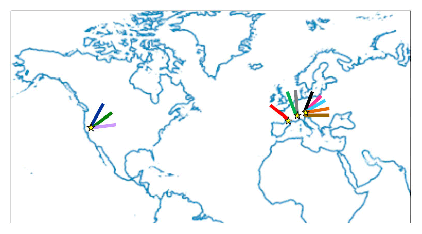
Figure 1The map shows the approximate location of the 11 spatial snow depth data sets. The colors of the trays indicate the region, measurement platforms or acquisition date as presented in Fig. 2.

Figure 2Probability density functions for fine-scale (a) snow depth, (b) elevation and (c) squared-slope-related parameter per observation data set in its original horizontal resolution, i.e., between 0.1 and 3 m. Densities were normalized with the corresponding maximum density of all data sets. Note that for elevation (b) the y axis was cut for better visibility. Colors represent the different geographic regions, measurement platforms or acquisition dates (number) of the compiled data set as indicated in Sect. 2.1 to 2.4.
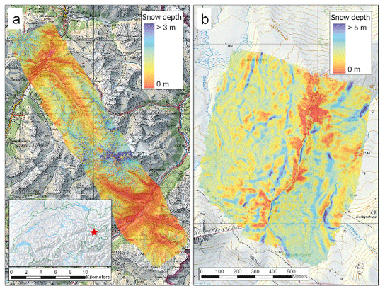
Figure 3Snow depth maps of the eastern Swiss Alps: (a) in the Dischma region (ALS data) and (b) at Gaudergrat (UAS data) at the peak of winter. The red dot in the inset map for Switzerland shows the location of the two sites. Pixmap © 2020 Swisstopo (5704000000), reproduced with the permission of Swisstopo (JA100118).
2.1 Eastern Swiss Alps
We used snow depth data sets acquired by three different platforms at four different alpine sites in the eastern Swiss Alps.
The first platform was airborne digital scanning (ADS) using an optoelectronic line scanner on an airplane. Data were acquired from the Wannengrat and Dischma areas near Davos in the eastern Swiss Alps (Bühler et al., 2015). ADS-derived snow depth data sets were used from 20 March 2012 (“ads-CH2”) to 9 March 2016 (“ads-CH1”), together with summer digital elevation models (DEMs) (Marty et al., 2019). The data set covers about 150 km2 at 2 m resolution. Bühler et al. (2015) validated the 2 m ADS-derived snow depth data among others with TLS data. They obtained a root mean square error (RMSE) of 33 cm and a normalized median absolute deviation (NMAD) of the residuals (Höhle and Höhle, 2009) of 26 cm.
The second platform was an unmanned aerial system (UAS) recording optical imagery with real-time kinematic (RTK) positioning of the image acquisition points of the snow cover with a standard camera over two different smaller regions near Davos in the eastern Swiss Alps (Bühler et al., 2016; Eberhard et al., 2021). These images were photogrammetrically processed into a digital surface model (DSM). By subtracting the snow-free DSM from the winter flight, the HS values were obtained (Bühler et al., 2017). An UAS-derived snow depth data set was used from 7 April 2018 (“uav-CH9”) from Schürlialp, together with a UAS-acquired summer DEM (Eberhard et al., 2021). The Schürlialp data set covers about 3.2 km2 which we used at 30 cm resolution. A second UAS-derived snow depth data set was used from 29 March 2019 (“uav-CH8”) from Gaudergrat, together with a UAS-acquired summer DEM. The Gaudergrat data set covers about 0.8 km2 at 10 cm resolution (Fig. 3b). Compared to snow depth data from snow probing, Eberhard et al. (2021) obtained an RMSE of 16 cm and a NMAD of 11 cm for UAS-derived snow depth data at 9 cm horizontal resolution from Schürlialp.
The third platform was airborne laser scanning (ALS) above the Dischma region near Davos in the eastern Swiss Alps (Fig. 3a). This acquisition was a Swiss partner mission of the Airborne Snow Observatory (ASO) (Painter et al., 2016). For consistency reasons, the same lidar setup was used, and similar processing standards to the ASO campaigns in California were applied (Sect. 2.2). ALS-derived snow depth data were used from 20 March 2017 (“als-CH3”), together with a summer DEM from 2017. The ALS data set from Switzerland used here covers about 260 km2 at 3 m resolution. Details on the derivation of the ALS data can be found in Mazzotti et al. (2019), though this study focused on three 0.5 km2 forested sub-data sets. Validation of 1 m ALS-derived snow depth grids from 20 March 2017 against data from snow probing within the forest but outside the canopy (i.e., not below a tree) resulted in an RMSE of 13 cm and a bias of −5 cm.
2.2 The Sierra Nevada, CA, US
We used data sets acquired by two different platforms above Tuolumne basin in the Sierra Nevada (California) in the US.
The first platform was ALS performed by ASO (Painter et al., 2016). ALS-derived snow depth data were used from 26 March 2016 (“als-US7”) and 2 May 2017 (“als-US6”), together with a summer DEM (Painter, 2018). The second platform was a Pléiades product from 1 May 2017 (“plei-US6”). A detailed data description of the Pléiades data set derivation is given in Deschamps-Berger et al. (2020).
We used the ASO summer DEM for the Pléiades, as well as the ALS snow depth data sets. Given that the extent of the Pléiades snow depth data set was much smaller than the ALS domain, we cropped the ALS data sets to the Pléiades data set extension resulting in a coverage of about 280 km2. The horizontal resolution used here was 3 m for both data sets. Compared to snow probe measurements in relatively flat areas, ALS snow depth data at 3 m horizontal resolution was found unbiased with an RMSE of 8 cm (Painter et al., 2016). Pléiades-derived snow depth data were recently validated with ASO data over 137 km2 at 3 m resolution above Tuolumne basin (Deschamps-Berger et al., 2020). An RMSE of 80 cm, a NMAD of 69 cm and a mean bias of 8 cm were obtained for the Pléiades data set.
2.3 Eastern French Pyrenees
A Pléiades product was acquired over the Bassiès basin in the northeastern French Pyrenees. Pléiades-derived snow depth data were used from 15 March 2017 (“plei-FR4”), together with a summer DEM (Marti et al., 2016). The data set we used covers about 113 km2 at 3 m resolution. Marti et al. (2016) derived a median of the bias between 2 m Pléiades data and snow probe measurements of −16 cm and with UAS measurements of −14 cm. They further obtained a NMAD of 45 cm with snow probe measurements and a NMAD of 78 cm with UAS measurements.
2.4 Southeastern French Alps
TLS-derived snow depth data were acquired at two alpine mountain passes in the southeastern French Alps. One snow depth data set was acquired over Col du Lac Blanc on 9 March 2015 (“tls-FR10”) (Revuelto et al., 2020). A site and data description can be found in Naaim-Bouvet et al. (2010), Vionnet et al. (2014), and Schön et al. (2015, 2018). We used a UAS-acquired summer DEM (Guyomarc'h et al., 2019). The data set covers about 0.6 km2 at 1 m resolution. The second TLS-derived snow depth data set was acquired over Col du Lautaret at 27 March 2018 (“tls-FR5”) (Revuelto et al., 2020). We used a TLS-acquired summer DEM. The data set covers about 0.14 km2 at 1 m resolution. Previously, mean biases between 4 and 10 cm for TLS laser target distances up to 500 m were obtained between TLS-derived and reference tachymetry measurements (Prokop, 2008; Prokop et al., 2008; Grünewald et al., 2010).
2.5 Preprocessing
In all data sets, grid cells Δx with forest, rivers, glaciers or buildings were masked out. In order to avoid introducing any biases, we consistently neglected fine-scale snow depth values in all data sets that were lower than 0 m or larger than 15 m. We used a snow depth threshold of 0 m to decide whether or not a fine-scale grid cell was snow-covered.
We parameterize the standard deviation of snow depth σHS to reassess the validity of the fSCA parameterization for complex topography from Helbig et al. (2015) for a range of spatial scales, in particular for sub-kilometer spatial scales.
3.1 Fractional snow-covered area parameterization
Helbig et al. (2015) derived an fSCA parameterization by integrating a normal pdf assuming spatially homogeneous melt. Subsequent fitting over a range of coefficients of variation CV (standard deviation divided by its mean) between 0.06 and 1.00 resulted in a similar closed form fit for fSCA as Essery and Pomeroy (2004) obtained by integrating a lognormal pdf,
using current HS and the standard deviation of previous maximum snow depth or peak of winter. The standard deviation of snow depth at the peak of winter was derived by relating the peak of winter high-resolution spatial snow depth data from Switzerland and Spain to underlying summer terrain parameters (Helbig et al., 2015):
with a=0.549, b=0.309, HS and terrain correlation length ξ are in meters, and ξ and μ are summer terrain parameters, where μ is related to the mean squared slope via using partial derivatives of subgrid terrain elevations z, i.e., from a DEM. The correlation length ξ or typical width of topographic features in a domain size L was derived via with the standard deviation of elevations σz. The ratio indicates how many characteristic topographic features of length scale ξ are included in each L. Figure 2 in Helbig et al. (2009) shows a transect of a topography indicating the described characteristic length scales. Similar to Helbig et al. (2015), we linearly detrended the summer DEM before deriving the terrain parameters to unveil the correct terrain characteristics associated with the shaping process of the snow depth distribution at the corresponding scale. Using Eq. (1), fSCA can thus be derived with grid cell mean snow depth from a snow model and grid cell mean subgrid terrain parameters derived from a fine-scale summer DEM. With the σHS formulation shown in Eq. (2), Helbig et al. (2015) extended the fSCA parameterization (Eq. 1) for mountainous terrain.
3.2 Aggregating and pooling of data sets
Pooling all snow depth data sets yields a data pool with a vast variety in snow climates, topographic characteristics and thus snow depth distributions. We first aggregated all snow data in squared domain sizes L in regular grids between 3 m and 5 km covering each geographic site. Our choice of the smallest applicable L in a data set was defined by a large enough ratio (here ≥ 20) to minimize the influence of grid cell resolutions when spatially averaging (Helbig et al., 2009). When aggregating, we required at least 70 % valid data in a domain size which was the maximum threshold to obtain a sufficient number of domains for the largest domain sizes L of 3 m to 5 km. In addition to that, we excluded L with spatial mean slope angles larger than 60∘ and spatial mean snow depth HS lower than 5 cm. By applying these limitations and since horizontal resolutions Δx, as well as the overall extent of the data sets, vary, the full range of L values, consisting of 41 different L values, was not represented by each data set. Overall, this resulted in a pool of 367 643 domains with L values between 3 m and 5 km. We obtain a decreasing number of domains for increasing L with a range between 59 376 for L=90 m and 17 for L=5000 m (Fig. 4). Spatial averages and standard deviations were built for each L. The resulting pooled data set shows a large variability in summer terrain characteristics. Spatial average slope angles range from 4 to 60∘ (μ from 0.05 to 1.22; Fig. 5c), terrain correlation lengths ξ from 6 to 775 m and -ratios from 3 to 40. Thus, typical summer terrain characteristics captured by coarse climate model grid cells are well represented. The diversity of the remaining domains with regards to snow depth is shown by means of the pdfs for spatial mean HS and σHS as a function of domain size L in Fig. 5a and b. Since the data pool also covers a broad range in spatial mean HS (from 5 cm to 12.4 m) and spatial variability in snow depth σHS (from 1 cm to 4.6 m) (Fig. 5a and b), we assume interannual snow depth variability is well described. In the following, overbars are neglected for spatial averages, i.e., for instance HS represents spatial mean snow depth exclusively.
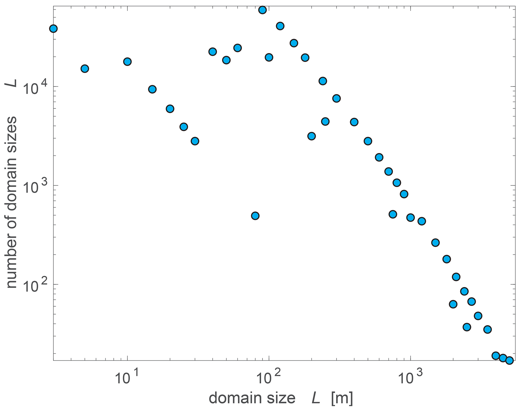
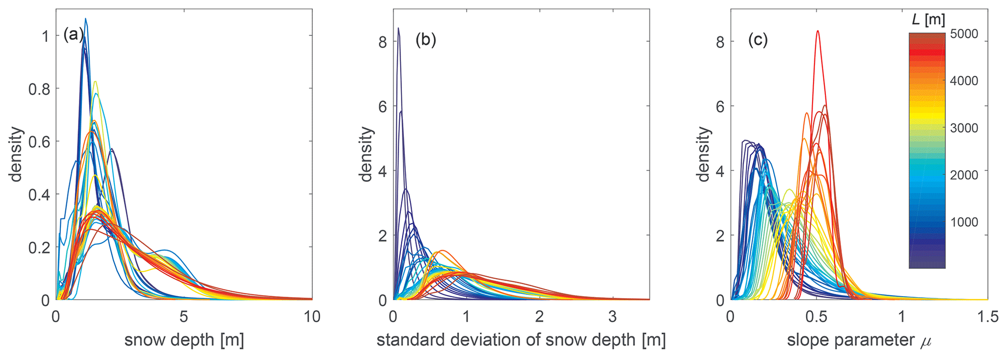
Figure 5Probability density functions for (a) snow depth, (b) standard deviation of snow depth and (c) squared-slope-related parameter per domain size L after preprocessing, pooling all data sets and building spatial averages.
3.3 Autocovariances for scale breaks
The spatial autocovariance allows us to find spatial scale breaks up to which snow depth values are highly correlated, i.e., up to which length scale the snow depth distribution is strongly dictated by local topographic interactions of the snow cover with wind, precipitation and radiation. Below this scale, break process models should ideally explicitly resolve these interactions to reliably describe the spatial snow depth distribution. Above this scale break, we assume that dominant wind or precipitation patterns due to larger-scale topography impacts dictate spatial snow depth distributions. At this scale range, the normalized standard deviations of snow depth σHS start leveling out (Fig. 6a), as well as the normalized variability in σHS among similarly sized L (Fig. 6b).
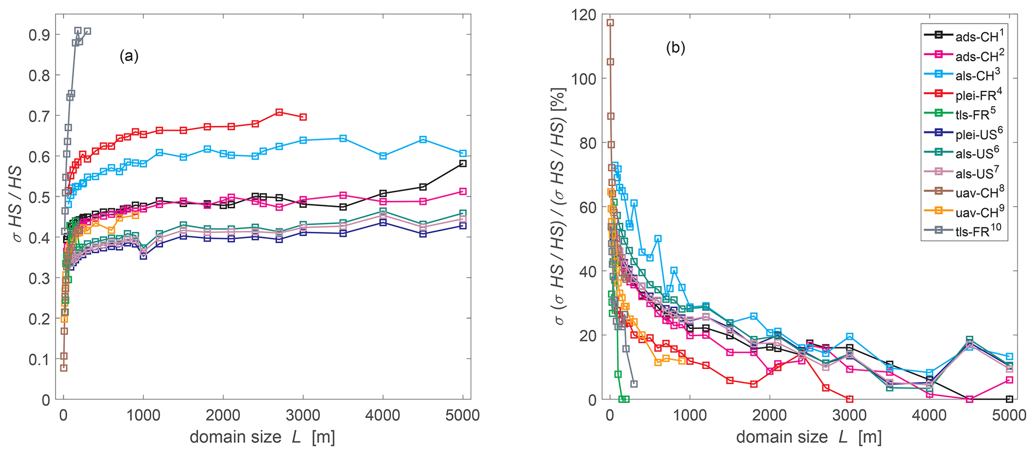
Figure 6(a) Normalized standard deviation of HS as a function of domain size L for each data set separately. (b) Normalized percentage of standard deviation of panel (a) among each L. L ranges from 3 m to 5 km. Colors represent the different geographic regions, measurement platforms or acquisition dates (number) of the compiled data set as indicated in Sect. 2.1 to 2.4.
We calculated spatial autocovariances for snow depth data sets with the fast Fourier transform (FFT), which allows for the computing of spatial autocovariances up to large distances by keeping the fine grid cell resolutions. We used the R function fft() of the “stats” package (see R Core Team, 2020). For each autocovariance, we then determine scale breaks using the R function uik() of the “inflection” package (R Core Team, 2020).
3.4 Deriving a new scale-independent fractional snow-covered area parameterization
Helbig et al. (2015) showed that fSCA performances increased with spatial scale and yielded their best performance for spatial scales larger than 1000 m. Since the fSCA parameterization was empirically developed on snow depth data from two geographic regions, here we reevaluated the scaling variables for the spatial variability in snow depth σHS, as well as the functional form of the parameterization using the much larger compiled HS data set of this study. Various scaling variables were previously employed to capture σHS in mountainous terrain. Helbig et al. (2015) selected HS, the squared-slope-related parameter μ and the ratio (Eq. 2). Skaugen and Melvold (2019) used HS and the standard deviation of the squared slope, with sqS being derived using sqS=tan 2ζ, where ζ is the slope angle in radians. Since tan 2ζ is the same as 2μ2 (e.g., Löwe and Helbig, 2012), we here derive sqS from 2μ2. Several other studies used σz as terrain parameter (e.g., Roesch et al., 2001). Here, we were interested in finding dominant scaling variables that correlate consistently across scales with σHS. We therefore analyzed the Pearson correlation coefficient r between various candidate parameters and σHS as a function of spatial scale, i.e., domain size L. Based on the results of previous studies, we selected the following candidate parameters: HS, μ, sqS, σsqS, and σz.
3.5 Performance measures
The performance in this article is evaluated by the following measures: the root mean square error (RMSE), normalized root mean square error (NRMSE; normalized by the range of measured data – max-min – or the mean of the measurements for fSCA), mean absolute error (MAE), the mean absolute percentage error (MAPE; absolute bias with measured minus parameterized and normalized with measurements), the mean percentage error (MPE; bias with measured minus parameterized and normalized with measurements) and the Pearson correlation coefficient r as a measure for correlation. We also evaluate the performances by deriving the two-sample Kolmogorov–Smirnov test (K-S test) statistic values D (Yakir, 2013) for the pdfs and by computing the NRMSE for quantile–quantile plots (NRMSEquant; normalized by the range of measured quantiles, max-min) for probabilities with values in the range of [0.1,0.9].
4.1 Spatial correlation range from snow depth data
We derived a total of 40 autocovariances for the available domain sizes L of 3 km with grid cell sizes Δx of 2 or 3 m. We obtained scale breaks between 183 and 681 m with a mean of 284 m (±σ 86 m) (Fig. 7). The zero crossings for each autocovariance were between 402 and 1815 m with a mean of 1011 m (±σ 402 m). For the mean autocovariance, we obtained a scale break at about 279 m and a zero crossing at about 1212 m. Based on the observed scale breaks, we selected a minimum length scale of 200 m for deriving a new scale-dependent fSCA parameterization for all larger scales. In the following, all results are therefore restricted to L≥ 200 m, leaving a pool of 41 249 domain sizes L with L between 200 m and 5 km for the development of the parameterization.
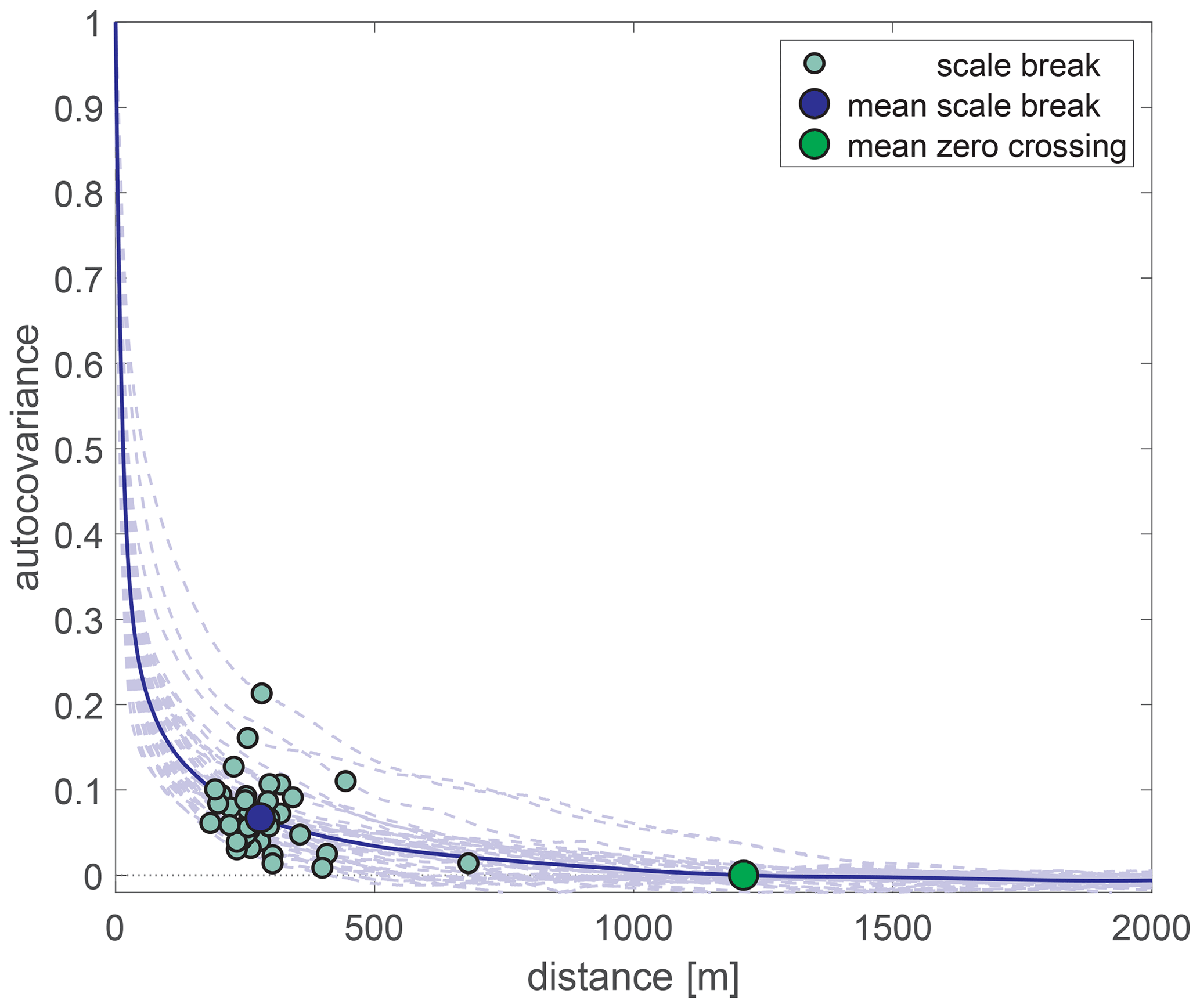
Figure 7FFT-derived autocovariances for spatial snow depth. Individual ranges, mean range and mean autocovariance zero crossing are shown.
4.2 Scaling variables for σHS
Correlation coefficients varied differently across spatial scales (Fig. 8a). For all scales, we obtained the largest correlation coefficients for HS ranging from 0.48 to 0.98 with a mean of 0.79. From correlations with the various subgrid terrain parameters, the largest correlations across all scales were reached for the squared-slope-related parameter μ ranging from 0.22 to 0.61 with a mean of 0.36. Similar consistent correlation coefficients across scales but slightly smaller for L≤ 1800 m resulted in the squared slope sqS having an overall mean of 0.33. The correlation coefficients for the standard deviation of sqS (σsqS) and σz were much less consistent across scales than for μ and sqS and were overall lower. The mean correlation for σsqS is 0.15, for 0.21 and for σz 0.01. Though the mean correlation between σHS and is rather low, the correlation remains more consistent across scales up to about 2500 m and increases for larger scales considerably up to 0.67 (cf. Fig. 8a).

Figure 8(a) Correlation coefficients between σHS and various parameters as a function of domain size L. (b) Standard deviation of snow depth σHS as a function of HS and μ.
We selected HS, μ and as main scaling parameters for σHS across spatial scales from 200 m to 5 km (Fig. 8b).
4.3 Scale-independent fSCA parameterization
The correlation analysis across scales revealed the same dominant correlation parameters as in Helbig et al. (2015). We therefore kept the functional form for σHS at the peak of winter suggested by Helbig et al. (2015) using the three scaling variables HS, μ and . The new σHS parameterization at the peak of winter thus has the same functional form than the one suggested by Helbig et al. (2015) which was presented in Eq. (2). However, the fit parameters a and b therein are replaced by the new parameters c and d which we specify below. To derive the new parameters c,d, we fitted nonlinear regression models by robust M-estimators using iterated reweighed least squares; see R (R Core Team, 2020) and its robustbase package version 0.93-6 (Maechler et al., 2020). We started at the scale length of 200 m, defined by the scale break which we derived before from spatial snow depth autocovariances.
Fit parameters were first derived for the entire data pool and L≥200 m yielding c=0.6589 (±0.0037) and d=0.5638 (±0.0043) with the 90 % confidence intervals of the fit parameters given in parentheses. These “new” constant parameters c,d are larger than the previously derived constants a,b in Eq. (2) (cf. Fig. 9).
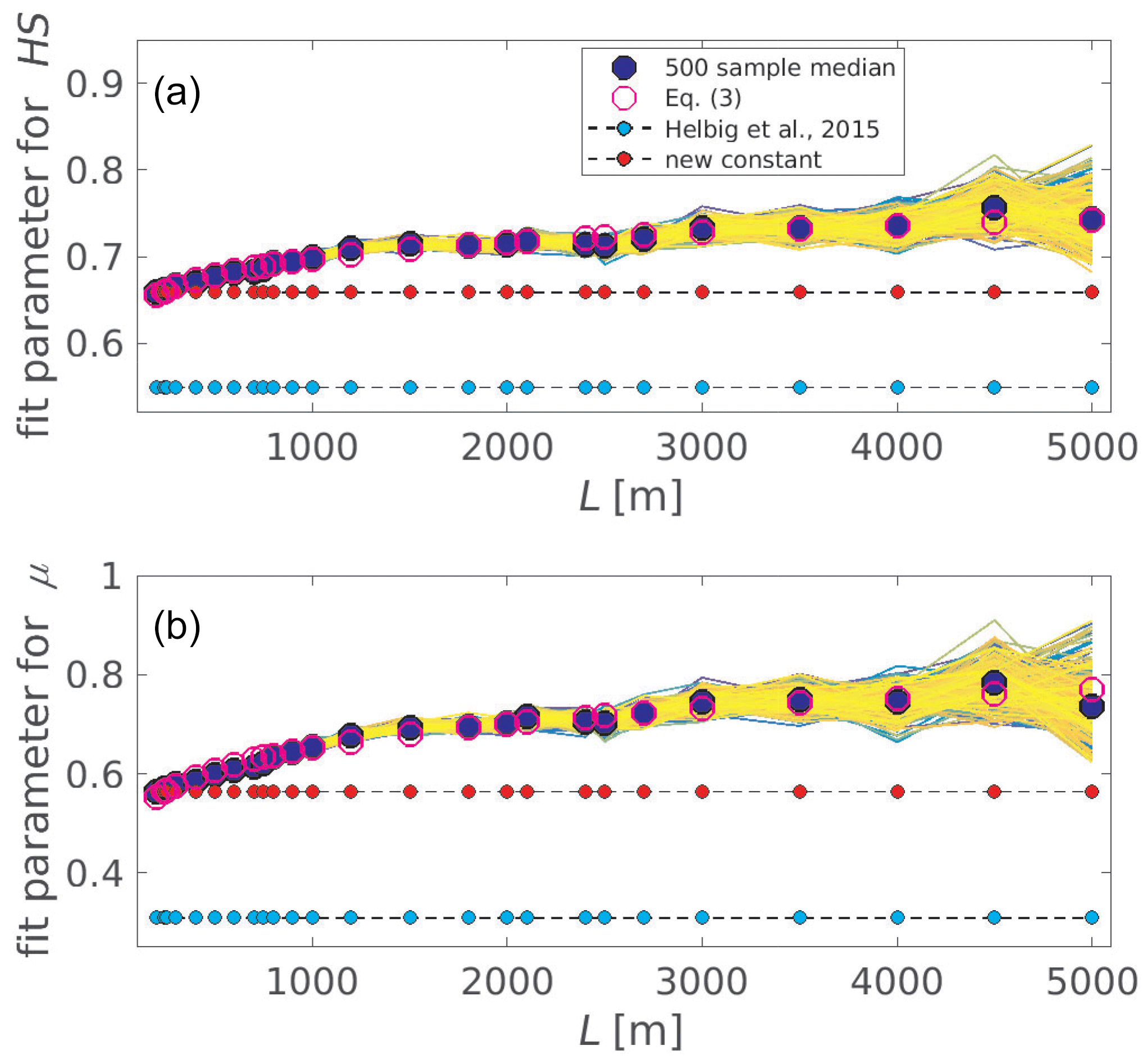
Figure 9Fit parameters for Eq. (2) as a function of domain sizes L to scale variables (a) HS and (b) μ. Colored lines show the fit parameters derived for each of the 500 random 80 % samples of each of the 25 sub-data pools. The dark blue dots depict the ensemble median per L. Previously obtained constant parameters of Helbig et al. (2015) (light blue dots) and newly fitted constant (red dots), as well as newly fitted scale-dependent (pink circles) parameters are shown.
In addition to fitting over the entire data pool and L≥ 200 m, we split the entire data pool into 25 sub-data pools for any available domain size between 200 m and 5 km (cf. Fig. 4). Thereby, each sub-data pool comprised all domains larger than or equal to the corresponding domain size, i.e., L≥ 200 m, L≥ 240 m, etc. Fitting over such a sub-data pool should allow us to describe the combined larger-scale topography–wind–precipitation impacts on the spatial snow depth distribution in mountainous terrain acting at scales larger than the observed scale break of about 200 m. From each of the 25 created sub-data pools, we randomly took 500 subsamples in which each subsample was restricted to 80 % data of the sub-data pool. Each of the 500 subsamples per sub-data pool was unique. Scale-dependent parameter values were derived for each of the 500 subsamples drawn from each of the 25 sub-data pools (cf. individual colored lines in Fig. 9). Given that the values of c,d clearly increase with spatial scale L (Fig. 9), we introduced L in c,d to improve the application of Eq. (2) across scales. By fitting the ensemble medians of all scale-dependent fit parameters (dark blue dots in Fig. 9) across all domain sizes between 200 m and 5 km, we obtained scale-dependent parameters c(L) and d(L). Thus, Eq. (2) using the following scale-dependent parameters c(L) and d(L) assembles our new σHS parameterization for L≥ 200 m:
with the 90 % confidence intervals of ±0.0097, ±0.0026 and ±0.0183, and ±0.0079 in the order of introduced constants in Eq. (3).
The new σHS parameterization using c(L) and d(L) (Eq. 2 with Eq. 3) is applied in the previously derived fSCA parameterization (Eq. 1). To demonstrate the resulting differences when using scale-dependent versus scale-independent fit parameters in parameterized σHS (Eq. 2), we will also validate the performance using constant c,d in the previously derived fSCA parameterization, as well as in the σHS parameterization.
4.4 Evaluation
4.4.1 Evaluation for σHS and fSCA for all L values
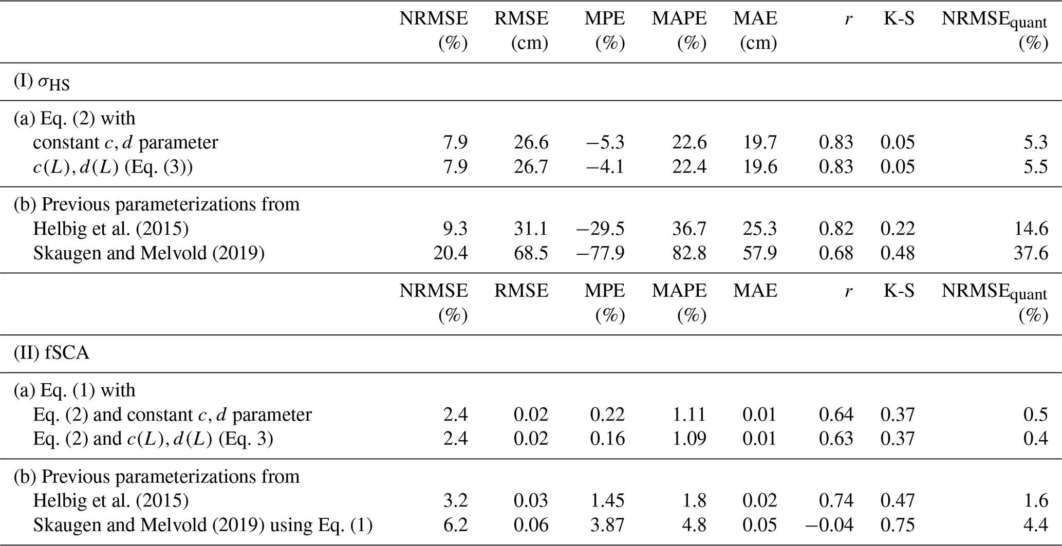
Parameterized σHS and fSCA perform well for all domain sizes, i.e., for L≥ 200 m, of the entire data pool. Very similar performance measures are obtained for the parameterizations using the newly derived constant fit parameters c,d and the parameterizations using the scale-dependent parameters c(L),d(L) (cf. Table 1 and Ia and IIa). We obtain a slightly better MPE for σHS when using scale-dependent fit parameters (−4 % versus -5 %); however, for fSCA, MPEs are the same (0.2 %). The same rather low NRMSE results for σHS (8 %) and for fSCA (2 %) are obtained when using constant or scale-dependent fit parameters.
Helbig et al. (2015)Skaugen and Melvold (2019)Helbig et al. (2015)Skaugen and Melvold (2019)Table 1Performance measures for all L values between measurement and parameterization of (I) standard deviation of snow depth σHS with (a) Eq. (2) and constant or L-dependent fit parameters c,d (Eq. 3) and (b) σHS as in Helbig et al. (2015) and Skaugen and Melvold (2019) and of (II) fSCA with (a) Eq. (1) and (1a) and (b) fSCA as in Helbig et al. (2015) and Skaugen and Melvold (2019) using Eq. (1).
4.4.2 Scale-dependent evaluation for σHS and fSCA
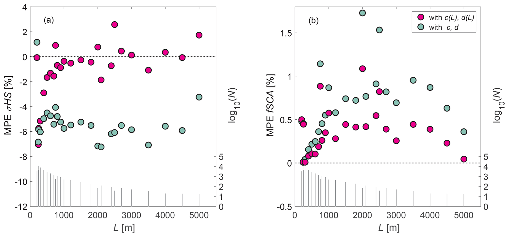
While mean performance measures of the σHS and fSCA parameterization are almost uninfluenced by using constant or scale-dependent fit parameters (cf. Table 1 and Ia and IIa), we found diverging performances when analyzing performance measures as a function of scale (Fig. 10). Across scales, improved or similar performances were achieved when using scale-dependent fit parameters in parameterized σHS, especially for larger scales. Maximum performance improvements for σHS of 4 % and for fSCA of 0.7 % occurred for L of 2500 m when using scale-dependent fit parameters. Thus, introducing scale-dependent fit parameters enhanced the σHS parameterization for application across scales.
4.4.3 Scale- and region-dependent evaluation for σHS and fSCA
A large data set from various geographic regions allows us to develop a more reliable empirical parameterization than being limited to the characteristics of a few data sets. Here, we not only compiled data sets from various geographic regions, but the data sets were also acquired by different measurement platforms coming with a range of inaccuracies between below 10 and 80 cm. As a consequence, larger scatter in performances appears when performance measures are depicted not only as a function of spatial scale but also regionwise, including platformwise. While most of the MPEs are still between −20 % and 10 %, some regions stand out because they have much larger MPEs when binned by scale, as well as by region (Fig. 11). For instance, a MPE of up to 60 % for σHS was obtained for TLS data from the southeastern French Alps, and overall larger MPEs, though consistent across scales, for the Pléiades data from the northeastern French Pyrenees were obtained. MPEs for fSCA on the other hand do not show a similar large spread among the regions and are low between −1 % to 2 % (Fig. 11b).
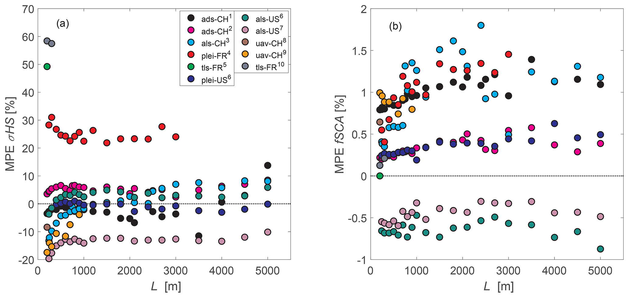
Figure 11Mean percentage error (MPE) as a function of L for the compiled data set for (a) σHS and (b) fSCA using Eqs. (1) to (3) with scale-dependent c(L),d(L). Colors represent the different geographic regions, measurement platforms or acquisition dates (number) of the compiled data set as indicated in Sect. 2.1 to 2.4.
4.4.4 Evaluation of previous closed form parameterizations
To increase our understanding of the performances achieved with the new parameterizations, we also tested two previously derived empirical parameterizations. Specifically, we investigated how parameterized σHS using Eq. (2) (Helbig et al., 2015) and using the recently published formulation of Skaugen and Melvold (2019) compare to observed σHS of our compiled data set (Fig. 12a). We further tested both σHS parameterizations in the fSCA parameterization (Eq. 1; Fig. 12b). The parameterization of Helbig et al. (2015) works well. The performance measures for all L values are only slightly worse compared to the new parameterizations using both constant and scale-dependent fit parameters (Table 1). However, compared to the performance measures for the parameterization of Skaugen and Melvold (2019), the performances of Helbig et al. (2015) are clearly improved. Though MPEs of both previous σHS parameterizations are scale-dependent, the MPEs of Skaugen and Melvold (2019) reveal a larger scale-dependency of the performances compared to Helbig et al. (2015) (Fig. 12a). In particular, individual MPEs vary a lot from MPEs for all L values given in Table 1.
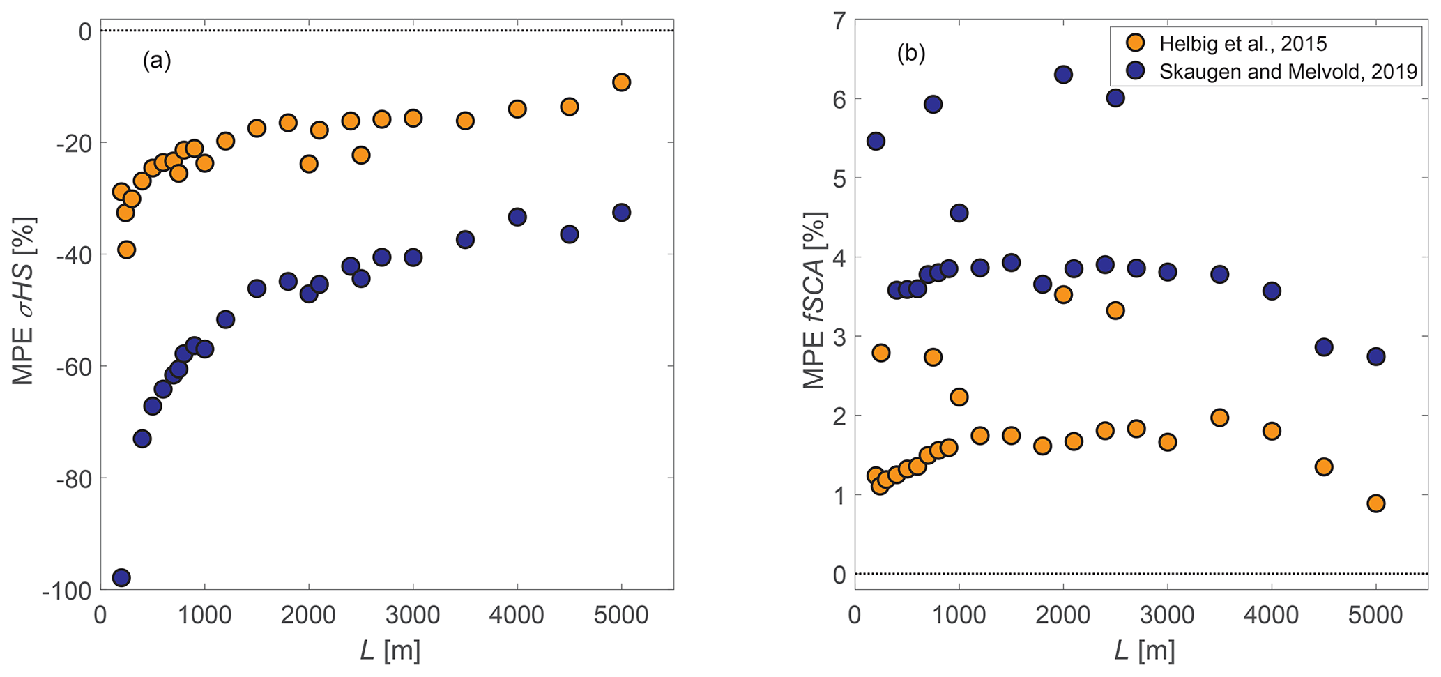
Figure 12Mean percentage error (MPE) as a function of L for the compiled data set for (a) σHS and (b) fSCA. MPEs are shown for the σHS and fSCA parameterizations of Helbig et al. (2015), as well as for the σHS parameterization of Skaugen and Melvold (2019) and the σHS parameterization of Skaugen and Melvold (2019) applied in the fSCA parameterization of Helbig et al. (2015) (Eq. 1).
5.1 Spatial correlation range
While multiscale behavior for spatial snow depth data has been found in various studies, observed scale breaks depend on the extent and horizontal resolution of the investigated snow depth data sets. A first scale break of spatial snow depth data in treeless, alpine terrain has been observed between 10 to 20 m (e.g., Deems et al., 2006; Trujillo et al., 2007; Schweizer et al., 2008; Schirmer and Lehning, 2011; Helfricht et al., 2014; Mendoza et al., 2020), and a second scale break has been observed at around 60 m (Trujillo et al., 2009). By computing spatial autocovariances starting with domain sizes L of 200 m at 0.1 to 1 m resolution and increasing up to 3 km at 2 to 3 m resolution, we also detected the two previously found scale breaks (not shown). However, by additionally covering larger spatial extents than have been previously investigated, we also detected a third scale break with a mean at about 280 m (Fig. 7). Similar long-range scale breaks between 185 and 300 m were very recently reported from analyzing 24 TLS-derived snow depth data sets acquired during six snow seasons in a subalpine catchment in the Spanish Pyrenees (Mendoza et al., 2020). Furthermore, a similar scale break at around 200 m was recently found by analyzing performance decreases in distributed snow modeling in various grid cell sizes, together with a semivariogram analysis of subgrid summer terrain slope angles in the same catchment in the High Atlas (Baba et al., 2019). While for other application studies, such as in avalanche forecasting, the smaller-scale breaks are decisive for explicitly describing the relevant snow-cover processes, here we are more interested in the largest detected scale break. Above scale lengths of 200 m, the longer-range processes of precipitation, wind and radiation interactions with topography most dominantly influence the spatial snow distribution in mountainous terrain, while we believe there are different physical processes which establish the smaller-scale breaks at around 10 to 20 and 60 m. The results presented here indicate that the model described by Eqs. (1) and (3) is reliably parameterizing the spatial snow distribution shaped by the longer-range precipitation, wind and radiation interactions with topography for spatial scales between 200 m and 5 km. Above the detected scale range of around 200 m, not only the spatial autocorrelations approach zero (Fig. 7), but normalized σHS clearly start leveling out, as well as the normalized variability in σHS among similarly sized L (Fig. 6). Thus, even though we could not verify the fSCA parameterization for length scales larger than 5 km, we believe that as long as grid cell mean slope angles are larger than zero, Eqs. (1) and (3) might also hold for larger grid cell sizes than 5 km.
5.2 Scaling parameter
We not only investigated dominant correlations between the spatial snow depth distribution and terrain parameters, but we also analyzed these correlations as a function of spatial scale. For some commonly applied scaling parameters, this revealed large variations in correlations across scales such as for σz (Fig. 8a). Similar to our results, Skaugen and Melvold (2019) also obtained large correlations between σHS and mean squared slope sqS for spatial snow depth data sets acquired at the peak of winter in Norway, though this was only analyzed for grid cells of 0.5 km2 (0.5 km × 1 km). Nevertheless, this confirms our findings since mean squared slope is related to the slope-related parameter μ used here by sqS=2μ2. However, Skaugen and Melvold (2019) obtained a slightly improved correlation for the standard deviation of squared slope and therefore selected this parameter to stratify the topography for parameterizing σHS. Across spatial scales, as well as for all L values, we obtained lower correlations between the standard deviation of squared slope and σHS, though we observed cross-correlations between the mean and the standard deviation of squared slope of 0.71, indicating that both parameters correlate well with σHS.
5.3 Scale-independent fSCA parameterization
The closed form fractional snow-covered area parameterization fSCA given in Eq. (1) got enhanced by recalibration and introducing scale-dependent fit parameters (Eq. 3) to make the performance consistent across spatial scales.
We developed the parameterization on a large snow depth data set. Large variability in the snow depth data set was gained by compiling 11 individual data sets from varying geographic regions, as well as various measurement platforms. While the latter might explain the remaining performance differences discussed below, the first led to large variability in summer terrain characteristics and snow climates and consequently spatial snow depth distributions (cf. Fig. 2). Though our presented parameterization for σHS was empirically derived, it is reassuring that for a new empirical derivation on a much larger and more diverse snow depth data set, the same underlying functional form could be used. Furthermore, larger (about 17 % and 45 %) but overall consistent constant fit parameters were obtained compared to those from Helbig et al. (2015) based on a more limited number of data sets and just two geographic regions (cf. a and b in Eq. 2 and c,d presented in Sect. 4.3 or Fig. 9).
In addition to deriving constant fit parameters across spatial scales, we took 500 random 80 % subsamples from each of the 25 sub-data pools (Sect. 4.3). Scale-dependent constants considerably increased with increasing scale from L = 200 m to L = 5 km by at most 12 % and 38 %, respectively (Fig. 9). This demonstrates that accounting for scale-dependent constants in the fSCA parameterization (Eq. 1 with Eqs. 2 and 3) had to be done. While we did not split our data set in development and validation subsets, fitting over the ensemble median of all scale-dependent parameters to derive c(L),d(L) ensures confidence in the resulting fit parameters.
An increase in scatter among all c(L) and d(L) with increasing domain scale L (Fig. 9) can be most likely explained by a concurrent decrease in available valid data in larger L values. Though we required at least 70 % valid data per L when aggregating fine-scale snow depth data in domain sizes L, the maximum threshold of 70 % was more often required for the larger L values than for smaller L values.
5.4 Evaluation
5.4.1 Evaluation for σHS and fSCA
Upon deriving performance measures on parameterized and observed σHS and fSCA for all L values (i.e., the pooled performance), we obtained very similar performances when using newly derived constant or scale-dependent fit parameters, i.e., c,d or c(L),d(L) (Table 1). Despite considerable differences up to 12 % for c and up to 38 % for d between constant and scale-dependent fit parameters (Fig. 9), pooled performances for all L values for σHS and fSCA were similar (Table 1). An explanation for this is that the number of available domains is strongly decreasing with increasing L. For L≥ 3000 m, we have only about 0.33 % (137 in total) valid domains available compared to the total of 41 249 for L< 3000 m (Fig. 4). This emphasizes the need for a scale-dependent evaluation.
5.4.2 Scale-dependent evaluation for σHS and fSCA
The largest improvement in MPE for all L values seems to originate from the recalibration using the new compiled data set with a reduction in MPE from −30 % to −5 % compared to a reduction from −5 % to −4 % when introducing scale-dependent fit parameters (Table 1). However, MPEs as a function of scale clearly demonstrated the improved behavior when using scale-dependent c(L),d(L) instead of constant fit parameters c,d in the σHS and fSCA parameterization (Fig. 10). Given that constant c,d were fitted over the entire data set as have been c(L),d(L), any performance improvement using c(L),d(L) instead of constant c,d for parameterized σHS and fSCA originates in introducing scale-dependent parameters. For the parameterizations using the constant fit parameters c,d, errors varied slightly more across scales than when using the scale-dependent c(L),d(L) version. Individual scale-dependent errors were in part larger than the MPEs for all L values given in Table 1. Unequal numbers of valid domains per L most likely also contributed to this.
5.4.3 Scale- and region-dependent evaluation for σHS and fSCA
While we did not perform an evaluation using independent snow depth data sets, studying regionwise performances reveals the spread in errors we can expect when the new parameterizations are applied on an individual independent data set (Fig. 11). We obtain much larger positive MPEs for σHS at lower spatial scales of L= 200 m and L= 300 m for the two TLS data sets in the southeastern French Alps and overall larger MPEs between 20 % and 30 %, though consistent across scales, for the Pléiades data from the Bassiès basin in the northeastern French Pyrenees. It is unclear if these larger MPEs originate in uncertainties of the data acquisition, i.e., are platform specific, or if they are linked to spatial snow depth distributions which could not be captured by the proposed new parameterizations. RMSEs for the various remote sensing platforms and data sets used here (Sect. 2) decrease from 80 cm for Pléiades data from the Sierra Nevada to 33 cm for the ADS, to 16 cm for UAS, to 13 cm for ALS data from Switzerland, to 8 cm for ALS data from the Sierra Nevada and to 4 to 10 cm for TLS data in general. Given the rather low errors typically obtained for TLS data compared to the other remote sensing platforms, the reason for the large deviations in the TLS data sets might not originate in inaccuracies of the data acquisition. On the contrary, the observed bias in the Pléiades data from the northeastern French Pyrenees might indeed be attributed to the rather large inaccuracies of the platform with NMADs of 45 to 78 cm (Marti et al., 2016). However, Pléiades data from the Sierra Nevada come with a similarly large NMAD of 69 cm, but σHS can be parameterized very well with MPEs lower than ±3 % across spatial scales (Fig. 11a). Observed σHS from the TLS, as well as from the Pléiades data in France, was considerably larger than parameterized σHS, but mean slope angles alone can also not explain this behavior (between 6 and 23∘ for the TLS data and between 13 and 50∘ for the Pléiades data).
While we were not able to clearly relate some of the poorer regionwise performances to uncertainties related to the platform, other studies entirely focused on performing extensive intercomparisons between platforms for large-scale snow depth mapping in alpine terrain (e.g., Bühler et al., 2015, 2016; Eberhard et al., 2021; Deschamps-Berger et al., 2020).
5.4.4 Evaluation of previous closed form parameterizations
Though we developed a new σHS parameterization (Eq. 3), empirically derived parameterizations can only describe the variability inherent in the data set used to derive the parameterization. In addition to the regionwise evaluation, analyzing performances of previous empirically derived parameterizations may therefore allow us to estimate expected performance sensitivity to independent data sets. While both tested parameterizations of σHS (Helbig et al., 2015; Skaugen and Melvold, 2019) showed a worse performance than the new parameterizations and less consistency as a function of scale, the model performances of Helbig et al. (2015) were only slightly worse than the new parameterizations (Table 1). The parameterization for σHS of Skaugen and Melvold (2019) was developed on mean domain sizes L of 750 m, whereas Helbig et al. (2015) used L values between 50 m to 3 km. This difference might be one reason for the overall poorer performances of Skaugen and Melvold (2019) compared to Helbig et al. (2015) across spatial scales. Since only 1 out of the 11 data sets used in this study was previously used to develop the parameterization of Helbig et al. (2015), an overall similar performance of Helbig et al. (2015) (Fig. 12) with the large compiled data set of this study clearly confirms the underlying functional form of σHS suggested by Helbig et al. (2015) which was reapplied here.
We presented an empirical peak of winter parameterization for the standard deviation of snow depth σHS for treeless, mountainous terrain, describing the spatial snow depth distribution in a grid cell for various model applications. The scaling variables in the new parameterization of σHS and fSCA are the same as in Helbig et al. (2015) which are spatial mean snow depth, a squared-slope-related parameter and a terrain correlation length. All subgrid terrain parameters can be easily derived from fine-scale summer DEMs for each coarse grid cell.
By introducing spatial scale dependencies in the variables in the formulation for σHS of Helbig et al. (2015), σHS can be consistently parameterized across spatial scales starting at scales ≥200 m. The spatial snow depth variability or σHS is the important variable to parameterize the fractional snow-covered area or fSCA (Helbig et al., 2015). Performance improvements across spatial scales of the σHS parameterization therefore directly enhanced the fSCA parameterization. Between length scales of 200 m and 5 km, mean percentage errors (MPE) were between −7 % and 3 % for σHS and between 0 % and 1 % for fSCA.
The subgrid parameterization of σHS was developed from 11 spatial snow depth data sets from seven different geographic regions at high spatial resolutions between 0.1 to 3 m and with spatial coverage between 0.14 to 280 km2. An evaluation of two previously presented empirical σHS parameterizations confirmed the functional form of the parameterization of Helbig et al. (2015), as well as the need to enhance its performance across scales. By analyzing data from the large pool of spatial snow depth data sets, we were able to recalibrate the subgrid parameterization of σHS and achieve improved performances using new constant fit parameters. Additionally introducing a scale dependency in the dominant scaling variables further improved the performance across spatial scales. Mean MPEs of σHS over all scales (i.e., pooled performance) reduced from −30 % using Helbig et al. (2015) to −5 % after recalibration to −4 % after introducing scale-dependent fit parameters (Table 1). Individual scale-dependent improvements in MPEs reached up to 4 % when using newly derived scale-dependent fit parameters compared to newly derived constant fit parameters for σHS from the large data pool. This shows the improvement thanks to introducing scale-dependent parameters (Fig. 10). Towards estimating the possible spread in performances when applying empirically derived σHS and fSCA for independent geographic regions, we validated the parameterizations separately for each region and scale. While this clearly increased MPEs for three data sets, the majority of the region- and scale-dependent MPEs were between ±10 % for σHS and between −1 % and 1.5 % for fSCA, indicating that the parameterizations perform similarly well in most geographical regions.
By parameterizing peak of winter σHS in mountainous terrain, Helbig et al. (2015) extended the fSCA parameterization of Essery and Pomeroy (2004) for topography. Here, we extended peak of winter σHS parameterization, and thus the fSCA parameterization, to be applicable over a large range of snow climates and topographic characteristics, as well as across spatial scales. Since fSCA is an essential model parameter, a seasonal fSCA algorithm describing the variability throughout a winter season is of relevance for various model applications. A peak of winter parameterization of σHS that describes the maximum spatial snow depth variability can not, however, be used alone to describe that seasonal fSCA evolution. A reliable model application of any fSCA parameterization requires an implementation accounting for alternating snow accumulation and melt events during the season, i.e., to describe the SCD. Especially at lower elevations, the separation of the SCD in only one accumulation period followed by a melting period is no longer valid (Egli and Jonas, 2009). A description of an algorithm for a seasonal fSCA model implementation which uses the new scale-independent peak of winter parameterization of σHS in the fSCA parameterization presented here is currently in preparation. Extending the empirical peak of winter fSCA parameterization to a broader range of spatial scales and snow climates was thus a meaningful step towards accounting for spatiotemporal variability in snow depth for multiple snow model applications.
All data used in this study are described in the data section. The data can be downloaded from the referenced repositories, or data availability is described in the referenced publications.
YB, LE, CDB, SG, MD, JR, JSD and TJ were responsible for data acquisition and processing, experiment and platform design, and setup. NH was responsible for the development of the parameterization. All authors contributed to the paper with discussions and ideas. NH wrote the paper with contributions from all coauthors.
The authors declare that they have no conflict of interest.
We thank Vincent Vionnet, Yannick Deliot, Gilbert Guyomarc’h and Aymeric Richard for their effort in acquiring and processing TLS observations at Col du Lac Blanc. CNRM/CEN is part of Labex OSUG@2020 (investissement d’avenir – ANR10 LABX56). Pléiades imagery was acquired through DINAMIS (Dispositif Institutionnel National d’Approvisionnement Mutualisé en Imagerie Satellitaire). We further thank the two anonymous reviewers for the helpful comments on the manuscript.
Nora Helbig was funded by a grant of the Swiss National Science Foundation (SNF) (grant no. IZSEZ_186887), as well as partly funded by the Federal Office of the Environment (FOEN). Simon Gascoin was partly supported from CNES Tosca and Programme National de Télédétection Spatiale (PNTS) (grant no. PNTS-2018-4). Jesus Revuelto was funded by an AXA grant (grant no. CNRM 3.2.01/17) and by ANR JCJC EBON (grant no. ANR-16-CE01-0006).
This paper was edited by Carrie Vuyovich and reviewed by two anonymous referees.
Andreadis, K. M. and Lettenmaier, D. P.: Assimilating remotely sensed snow observations into a macroscale hydrology model, Adv. Water Resour., 29, 872–886, 2006. a
Baba, M. W., Gascoin, S., Kinnard, C., Marchane, A., and Hanich, L.: Effect of Digital Elevation Model Resolution on the Simulation of the Snow Cover Evolution in the High Atlas, Water Resour. Res., 55, 5360–5378, https://doi.org/10.1029/2018WR023789, 2019. a
Bellaire, S. and Jamieson, B.: Forecasting the formation of critical snow layers using a coupled snow cover and weather model, Cold. Reg. Sci. Technol., 94, 37–44, 2013. a
Bühler, Y., Marty, M., Egli, L., Veitinger, J., Jonas, T., Thee, P., and Ginzler, C.: Snow depth mapping in high-alpine catchments using digital photogrammetry, The Cryosphere, 9, 229–243, https://doi.org/10.5194/tc-9-229-2015, 2015. a, b, c
Bühler, Y., Adams, M. S., Bösch, R., and Stoffel, A.: Mapping snow depth in alpine terrain with unmanned aerial systems (UASs): potential and limitations, The Cryosphere, 10, 1075–1088, https://doi.org/10.5194/tc-10-1075-2016, 2016. a, b
Bühler, Y., Adams, M. S., Stoffel, A., and Boesch, R.: Photogrammetric reconstruction of homogenous snow surfaces in alpine terrain applying near-infrared UAS imagery, Int. J. Remote Sens., 38, 3135–3158, 2017. a
Clark, M. P., Hendrikx, J., Slater, A. G., Kavetski, D., Anderson, B., Cullen, N. J., Kerr, T., Hreinsson, E. O., and Woods, R. A.: Representing spatial variability of snow water equivalent in hydrologic and land-surface models: A review, Water Resour. Res., 47, W07539, https://doi.org/10.1029/2011WR010745, 2011. a
Deems, J. S., Fassnacht, S. R., and Elder, K. J.: Fractal Distribution of Snow Depth from Lidar Data, J. Hydrometeorol., 7, 285–297, 2006. a, b
Deschamps-Berger, C., Gascoin, S., Berthier, E., Deems, J., Gutmann, E., Dehecq, A., Shean, D., and Dumont, M.: Snow depth mapping from stereo satellite imagery in mountainous terrain: evaluation using airborne laser-scanning data, The Cryosphere, 14, 2925–2940, https://doi.org/10.5194/tc-14-2925-2020, 2020. a, b, c, d
Doms, G., Förstner, J., Heise, E., Herzog, H. J., Mironov, D., Raschendorfer, M., Reinhardt, T., Ritter, B., Schrodin, R., Schulz, J. P., and Vogel, G.: A Description of the Nonhydrostatic Regional COSMO Model, Part II: Physical Parameterization, LM F90 4.20 38, Consortium for Small-Scale Modelling, Deutscher Wetterdienst, Offenbach, Germany, 2011. a
Douville, H., Royer, J.-F., and Mahfouf, J.-F.: A new snow parameterization for the Météo-France climate model Part II: validation in a 3-D GCM experiment, Clim. Dyn., 1, 37–52, 1995. a, b, c
Drusch, M., Del Bello, U., Carlier, S., Colin, O., Fernandez, V., Gascon, F., Hoersch, B., Isola, C., Laberinti, P., Martimort, P., et al.: Sentinel-2: ESA's optical high-resolution mission for GMES operational services, Remote Sens. Environ., 120, 25–36, 2012. a
Eberhard, L. A., Sirguey, P., Miller, A., Marty, M., Schindler, K., Stoffel, A., and Bühler, Y.: Intercomparison of photogrammetric platforms for spatially continuous snow depth mapping, The Cryosphere, 15, 69–94, https://doi.org/10.5194/tc-15-69-2021, 2021. a, b, c, d, e
Egli, L. and Jonas, T.: Hysteretic dynamics of seasonal snow depth distribution in the Swiss Alps, Geophys. Res. Lett., 36, 2009. a
Essery, R. and Pomeroy, J.: Implications of spatial distributions of snow mass and melt rate for snow-cover depletion: theoretical considerations, Ann. Glaciol., 38, 261–265, https://doi.org/10.3189/172756404781815275, 2004. a, b, c, d, e, f, g, h, i
Essery, R., Morin, S., Lejeune, Y., and Ménard, C. B.: A comparison of 1701 snow models using observations from an alpine site, Adv. Water Resour., 55, 131–148, 2013. a
Gascoin, S., Hagolle, O., Huc, M., Jarlan, L., Dejoux, J.-F., Szczypta, C., Marti, R., and Sánchez, R.: A snow cover climatology for the Pyrenees from MODIS snow products, Hydrol. Earth Syst. Sci., 19, 2337–2351, https://doi.org/10.5194/hess-19-2337-2015, 2015. a
Gascoin, S., Grizonnet, M., Bouchet, M., Salgues, G., and Hagolle, O.: Theia Snow collection: high-resolution operational snow cover maps from Sentinel-2 and Landsat-8 data, Earth Syst. Sci. Data, 11, 493–514, https://doi.org/10.5194/essd-11-493-2019, 2019. a
Griessinger, N., Seibert, J., Magnusson, J., and Jonas, T.: Assessing the benefit of snow data assimilation for runoff modeling in Alpine catchments, Hydrol. Earth Syst. Sci., 20, 3895–3905, https://doi.org/10.5194/hess-20-3895-2016, 2016. a, b
Griessinger, N., Schirmer, M., Helbig, N., Winstral, A., Michel, A., and Jonas, T.: Implications of observation-enhanced energy-balance snowmelt simulations for runoff modeling of Alpine catchments, Adv. Water Resour., 133, 103410, https://doi.org/10.1016/j.advwatres.2019.103410, 2019. a
Grünewald, T., Schirmer, M., Mott, R., and Lehning, M.: Spatial and temporal variability of snow depth and ablation rates in a small mountain catchment, The Cryosphere, 4, 215–225, https://doi.org/10.5194/tc-4-215-2010, 2010. a
Grünewald, T., Stötter, J., Pomeroy, J. W., Dadic, R., Moreno Baños, I., Marturià, J., Spross, M., Hopkinson, C., Burlando, P., and Lehning, M.: Statistical modelling of the snow depth distribution in open alpine terrain, Hydrol. Earth Syst. Sci., 17, 3005–3021, https://doi.org/10.5194/hess-17-3005-2013, 2013. a
Grünewald, T., Bühler, Y., and Lehning, M.: Elevation dependency of mountain snow depth, The Cryosphere, 8, 2381–2394, https://doi.org/10.5194/tc-8-2381-2014, 2014. a
Guyomarc'h, G., Bellot, H., Vionnet, V., Naaim-Bouvet, F., Déliot, Y., Fontaine, F., Puglièse, P., Nishimura, K., Durand, Y., and Naaim, M.: A meteorological and blowing snow data set (2000–2016) from a high-elevation alpine site (Col du Lac Blanc, France, 2720 m a.s.l.), Earth Syst. Sci. Data, 11, 57–69, https://doi.org/10.5194/essd-11-57-2019, 2019. a
Helbig, N. and van Herwijnen, A.: Subgrid parameterization for snow depth over mountainous terrain from flat field snow depth, Water Resour. Res., 53, 1444–1456, https://doi.org/10.1002/2016WR019872, 2017. a
Helbig, N., Löwe, H., and Lehning, M.: Radiosity approach for the surface radiation balance in complex terrain, J. Atmos. Sci., 66, 2900–2912, https://doi.org/10.1175/2009JAS2940.1, 2009. a, b
Helbig, N., van Herwijnen, A., Magnusson, J., and Jonas, T.: Fractional snow-covered area parameterization over complex topography, Hydrol. Earth Syst. Sci., 19, 1339–1351, https://doi.org/10.5194/hess-19-1339-2015, 2015. a, b, c, d, e, f, g, h, i, j, k, l, m, n, o, p, q, r, s, t, u, v, w, x, y, z, aa, ab, ac, ad, ae, af, ag, ah, ai, aj, ak, al, am, an, ao, ap, aq
Helfricht, K., Schöber, J., Schneider, K., Sailer, R., and Kuhn, M.: Interannual persistence of the seasonal snow cover in a glacierized catchment, J. Glaciol., 60, 889–904, https://doi.org/10.3189/2014JoG13J197, 2014. a
Höhle, J. and Höhle, M.: Accuracy assessment of digital elevation models by means of robust statistical methods, ISPRS J. Photogramm., 64, 398–406, https://doi.org/10.1016/j.isprsjprs.2009.02.003, 2009. a
Horton, S. and Jamieson, B.: Modelling hazardous surface hoar layers across western Canada with a coupled weather and snow cover model, Cold. Reg. Sci. Technol., 128, 22–31, 2016. a
Huang, C., Newman, A. J., Clark, M. P., Wood, A. W., and Zheng, X.: Evaluation of snow data assimilation using the ensemble Kalman filter for seasonal streamflow prediction in the western United States, Hydrol. Earth Syst. Sci., 21, 635–650, https://doi.org/10.5194/hess-21-635-2017, 2017. a
Kirchner, P. B., Bales, R. C., Molotch, N. P., Flanagan, J., and Guo, Q.: LiDAR measurement of seasonal snow accumulation along an elevation gradient in the southern Sierra Nevada, California, Hydrol. Earth Syst. Sci., 18, 4261–4275, https://doi.org/10.5194/hess-18-4261-2014, 2014. a
Lehning, M., Völksch, I., Gustafsson, D., Nguyen, T., and Stähli, M.: ALPINE3D: A detailed model of mountain surface processes and its application to snow hydrology, Hydrol. Process., 20, 2111–2128, 2006. a
Liston, G. E.: Representing Subgrid Snow Cover Heterogeneities in Regional and Global Models, J. Climate, 17, 1391–1397, 2004. a
López-Moreno, J. I., Revuelto, J., Alonso-Gonzáles, E., Sanmiguel-Vallelado, A., Fassnacht, S. R., Deems, J., and Morán-Tejeda, E.: Using very long-range Terrestrial Laser Scanning to Analyze the Temporal Consistency of the Snowpack Distribution in a High Mountain Environment, J. Mt. Sci., 14, 823–842, 2017. a
Löwe, H. and Helbig, N.: Quasi-analytical treatment of spatially averaged radiation transfer in complex topography, J. Geophys. Res., 17, D19101, https://doi.org/10.1029/2012JD018181, 2012. a
Luce, C. H., Tarboton, D. G., and Cooley, K. R.: Sub-grid parameterization of snow distribution for an energy and mass balance snow cover model, Hydrol. Process., 13, 1921–1933, 1999. a, b
Maechler, M., Rousseeuw, P., Croux, C., Todorov, V., Ruckstuhl, A., Salibian-Barrera, M., Verbeke, T., Koller, M., Conceicao, E. L. T., and Anna di Palma, M.: robustbase: Basic Robust Statistics, r package version 0.93-6, available at: http://robustbase.r-forge.r-project.org/ (last access: 5 February 2021), 2020. a
Magand, C., Ducharne, A., Moine, N. L., and Gascoin, S.: Introducing Hysteresis in Snow Depletion Curves to Improve the Water Budget of a Land Surface Model in an Alpine Catchment, J. Hydrometeor., 15, 631–649, https://doi.org/10.1175/JHM-D-13-091.1, 2014. a, b
Magnusson, J., Gustafsson, D., Hüsler, F., and Jonas, T.: Assimilation of point SWE data into a distributed snow cover model comparing two contrasting methods, Water Resour. Res., 50, 7816–7835, 2014. a
Marks, D., Domingo, J., Susong, D., Link, T., and Garen, D.: A spatially distributed energy balance snowmelt model for application in mountain basins, Hydrol. Process., 13, 1935–1959, 1999. a
Marti, R., Gascoin, S., Berthier, E., de Pinel, M., Houet, T., and Laffly, D.: Mapping snow depth in open alpine terrain from stereo satellite imagery, The Cryosphere, 10, 1361–1380, https://doi.org/10.5194/tc-10-1361-2016, 2016. a, b, c, d
Marty, M., Bühler, Y., and Ginzler, C.: Snow Depth Mapping, EnviDat, https://doi.org/10.16904/envidat.62, 2019. a
Mazzotti, G., Currier, W. R., Deems, J. S., Pflug, J. M., Lundquist, J. D., and Jonas, T.: Revisiting Snow Cover Variability and Canopy Structure Within Forest Stands: Insights From Airborne Lidar Data, Water Resour. Res., 55, 6198–6216, 2019. a
Melvold, K. and Skaugen, T.: Multiscale spatial variability of lidar-derived and modeled snow depth on Hardangervidda, Norway, Ann. Glaciol., 54, 273–281, 2013. a
Mendoza, P. A., Musselman, K. N., Revuelto, J., Deems, J. S., Lopez-Moreno, J. I., and McPhee, J.: Interannual and Seasonal Variability of Snow Depth Scaling Behavior in a Subalpine Catchment, Water Resour. Res., 56, e2020WR027343, https://doi.org/10.1029/2020WR027343, 2020. a, b, c
Mudryk, L., Santolaria-Otín, M., Krinner, G., Ménégoz, M., Derksen, C., Brutel-Vuilmet, C., Brady, M., and Essery, R.: Historical Northern Hemisphere snow cover trends and projected changes in the CMIP6 multi-model ensemble, The Cryosphere, 14, 2495–2514, https://doi.org/10.5194/tc-14-2495-2020, 2020. a, b
Naaim-Bouvet, F., Bellot, H., and Naaim, M.: Back analysis of drifting-snow measurements over an instrumented mountainous site, Ann. Glaciol., 51, 207–217, https://doi.org/10.3189/172756410791386661, 2010. a
Nagler, T., Rott, H., Malcher, P., and Müller, F.: Assimilation of meteorological and remote sensing data for snowmelt runoffforecasting, Remote Sens. Environ., 112, 1408–1420, 2008. a
Niu, G. Y. and Yang, Z. L.: An observation-based formulation of snow cover fraction and its evaluation over large North American river basins, J. Geophys. Res., 112, D21101, https://doi.org/10.1029/2007JD008674, 2007. a, b
Painter, T.: ASO L4 Lidar Snow Depth 3m UTM Grid, Version 1, NASA National Snow and Ice Data Center Distributed Active Archive Center, Boulder, Colorado, USA, https://doi.org/10.5067/KIE9QNVG7HP0, 2018. a
Painter, T., Berisford, D., Boardman, J., Bormann, K., Deems, J., Gehrke, F., Hedrick, A., Joyce, M., Laidlaw, R., Marks, D., Mattmann, C., Mcgurk, B., Ramirez, P., Richardson, M., Skiles, S. M., Seidel, F., and Winstral, A.: The Airborne Snow Observatory: fusion of scanning lidar, imaging spectrometer, and physically-based modeling for mapping snow water equivalent and snow albedo, Remote Sens. Environ., 184, 139–152, https://doi.org/10.1016/j.rse.2016.06.018, 2016. a, b, c
Parajka, J. and Blöschl, G.: Validation of MODIS snow cover images over Austria, Hydrol. Earth Syst. Sci., 10, 679–689, https://doi.org/10.5194/hess-10-679-2006, 2006. a
Prokop, A.: Assessing the applicability of terrestrial laser scanning for spatial snow depth measurements, Cold Reg. Sci. Technol., 54, 155–163, https://doi.org/10.1016/j.coldregions.2008.07.002, 2008. a
Prokop, A., Schirmer, M., Rub, M., Lehning, M., and Stocker, M.: A comparison of measurement methods: terrestrial laser scanning, tachymetry and snow probing, for the determination of spatial snow depth distribution on slopes, Ann. Glaciol., 49, 210–216, 2008. a
Raleigh, M. S., Lundquist, J. D., and Clark, M. P.: Exploring the impact of forcing error characteristics on physically based snow simulations within a global sensitivity analysis framework, Hydrol. Earth Syst. Sci., 19, 3153–3179, https://doi.org/10.5194/hess-19-3153-2015, 2015. a
R Core Team: R: A Language and Environment for Statistical Computing, R Foundation for Statistical Computing, Vienna, Austria, available at: https://www.R-project.org (last access: 5 February 2021), 2020. a, b, c
Revuelto, J., López-Moreno, J. I., Azorin-Molina, C., and Vicente-Serrano, S. M.: Topographic control of snowpack distribution in a small catchment in the central Spanish Pyrenees: intra- and inter-annual persistence, The Cryosphere, 8, 1989–2006, https://doi.org/10.5194/tc-8-1989-2014, 2014. a
Revuelto, J., Billecocq, P., Tuzet, F., Cluzet, B., Lamare, M., Larue, F., Richard, A., Deliot, Y., Guyomarc'h, G., Vionnet, V., and Dumont, M.: Terrestrial Laser Scanner observations of snow depth distribution at Col du Lautaret and Col du Lac Blanc mountain sites, Zenodo, https://doi.org/10.5281/zenodo.3628203, 2020. a, b
Revuelto, J., Billecocq, P., Tuzet, F., Cluzet, B., Lamare, M., Larue, F., and Dumont, M.: Random forests as a tool to understand the snow depth distribution and its evolution in mountain areas, Hydrol. Process., 34, 5384–5401, https://doi.org/10.1002/hyp.13951, 2020. a
Roesch, A., Wild, M., Gilgen, H., and Ohmura, A.: A new snow cover fraction parameterization for the ECHAM4 GCM, Clim. Dyn., 17, 933–946, 2001. a, b, c, d
Schirmer, M. and Lehning, M.: Persistence in intra-annual snow depth distribution: 2. Fractal analysis of snow depth development, Water Resour. Res., 47, https://doi.org/10.1029/2010WR009429, 2011. a
Schirmer, M., Wirz, V., Clifton, A., and Lehning, M.: Persistence in intra-annual snow depth distribution: 1. Measurements and topographic control, Water Resour. Res., 47, W09516, https://doi.org/10.1029/2010WR009426, 2011. a
Schön, P., Prokop, A., Vionnet, V., Guyomarc'h, G., Naaim-Bouvet, F., and Heiser, M.: Improving a terrain-based parameter for the assessment of snow depths with TLS data in the Col du Lac Blanc area, Cold Reg. Sci. Technol., 114, 15–26, 2015. a
Schön, P., Naaim-Bouvet, F., Vionnet, V., and Prokop, A.: Merging a terrain-based parameter with blowing snow fluxes for assessing snow redistribution in alpine terrain, Cold Reg. Sci. Technol., 155, 161–173, 2018. a
Schweizer, J., Kronholm, K., Jamieson, B., and Birkeland, K.: Review of spatial variability of snowpack properties and its importance for avalanche formation, Cold Reg. Sci. Technol., 51, 253–272, 2008. a
Shaw, T. E., Gascoin, S., Mendoza, P. A., Pellicciotti, F., and McPhee, J.: Snow Depth Patterns in a High Mountain Andean Catchment from Satellite Optical Tristereoscopic Remote Sensing, Water Resour. Res., 56, e2019WR024880, https://doi.org/10.1029/2019WR024880, 2020. a
Skaugen, T. and Melvold, K.: Modeling the snow depth variability with a high‐resolution lidar data set and nonlinear terrain dependency, Water Resour. Res., 55, 9689–9704, https://doi.org/10.1029/2019WR025030, 2019. a, b, c, d, e, f, g, h, i, j, k, l, m, n, o, p, q, r, s
Su, H., Yang, Z. L., Niu, G. Y., and Dickinson, R. E.: Enhancing the estimation of continental-scale snow water equivalent by assimilating MODIS snow cover with the ensemble Kalman filter, J. Geophys. Res., 113, D08120, https://doi.org/10.1029/2007JD009232, 2008. a
Swenson, S. C. and Lawrence, D.: A new fractional snow-covered area parameterization for the Community Land Model and its effect on the surface energy balance, J. Geophys. Res.-Atmos., 117, D21107, https://doi.org/10.1029/2012JD018178, 2012. a, b, c
Tarboton, D. G. and Luce, C. H.: Utah Energy Balance Snow Accumulation and Melt Model(UEB), Computer model technical description and users guide, Utah Water Research Laboratory and USDA Forest Service Intermountain Research Station, available at: https://www.fs.fed.us/rm/boise/publications/watershed/rmrs_1996_tarbotond001.pdf (last access: 5 February 2021), 1996. a
Thirel, G., Salamon, P., Burek, P., and Kalas, M.: Assimilation of MODIS snow cover area data in a distributed hydrological model using the particle filter, Remote Sens., 5, 5825–5850, 2013. a, b
Trujillo, E., Ramírez, J. A., and Elder, K. J.: Topographic, meteorologic, and canopy controls on the scaling characteristics of the spatial distribution of snow depth fields, Water Resour. Res., 43, W07409, https://doi.org/10.1029/2006WR005317, 2007. a, b
Trujillo, E., Ramírez, J. A., and Elder, K. J.: Scaling properties and spatial organization of snow depth fields in sub-alpine forest and alpine tundra, Hydrol. Process., 23, 1575–1590, https://doi.org/10.1002/hyp.7270, 2009. a
Vionnet, V., Martin, E., Masson, V., Guyomarc'h, G., Naaim-Bouvet, F., Prokop, A., Durand, Y., and Lac, C.: Simulation of wind-induced snow transport and sublimation in alpine terrain using a fully coupled snowpack/atmosphere model, The Cryosphere, 8, 395–415, https://doi.org/10.5194/tc-8-395-2014, 2014. a
Vionnet, V., Etchevers, I. D., Lafaysse, M., Queno, L., Seity, Y., and E. Bazile, E.: Numerical weather forecasts at kilometer scale in the French Alps: Evaluation and application for snowpack modeling, J. Hydrometeorol., 17, 2591–2614, 2016. a, b
Voegeli, C., Lehning, M., Wever, N., and Bavay, M.: Scaling precipitation input to spatially distributed hydrological models by measured snow distribution, Front. Earth Sci., 4, 108, https://doi.org/10.3389/feart.2016.00108, 2016. a
Yakir, B.: Nonparametric Tests: Kolmogorov-Smirnov and Peacock, chap. 6, John Wiley & Sons, Ltd, 103–124, https://doi.org/10.1002/9781118720608.ch6, 2013. a
Yang, Z. L., Dickinson, R. E., Robock, A., and Vinnikov, K. Y.: On validation of the snow sub-model of the biosphere atmosphere transfer scheme with Russian snow cover and meteorological observational data, J. Climate, 10, 353–373, 1997. a, b, c, d, e