the Creative Commons Attribution 4.0 License.
the Creative Commons Attribution 4.0 License.
 | 20 Dec 2021
Impact of the melt–albedo feedback on the future evolution of the Greenland Ice Sheet with PISM-dEBM-simple
Maria Zeitz
Ronja Reese
Johanna Beckmann
Uta Krebs-Kanzow
Ricarda Winkelmann
Surface melting of the Greenland Ice Sheet contributes a large amount to current and future sea level rise. Increased surface melt may lower the reflectivity of the ice sheet surface and thereby increase melt rates: the so-called melt–albedo feedback describes this self-sustaining increase in surface melting. In order to test the effect of the melt–albedo feedback in a prognostic ice sheet model, we implement dEBM-simple, a simplified version of the diurnal Energy Balance Model dEBM, in the Parallel Ice Sheet Model (PISM).
The implementation includes a simple representation of the melt–albedo feedback and can thereby replace the positive-degree-day melt scheme. Using PISM-dEBM-simple, we find that this feedback increases ice loss through surface warming by 60 % until 2300 for the high-emission scenario RCP8.5 when compared to a scenario in which the albedo remains constant at its present-day values. With an increase of 90 % compared to a fixed-albedo scenario, the effect is more pronounced for lower surface warming under RCP2.6. Furthermore, assuming an immediate darkening of the ice surface over all summer months, we estimate an upper bound for this effect to be 70 % in the RCP8.5 scenario and a more than 4-fold increase under RCP2.6. With dEBM-simple implemented in PISM, we find that the melt–albedo feedback is an essential contributor to mass loss in dynamic simulations of the Greenland Ice Sheet under future warming.
- Article
(3533 KB) - Full-text XML
-
Supplement
(335 KB) - BibTeX
- EndNote


The Greenland Ice Sheet is currently one of the main contributors to sea level rise (Frederikse et al., 2020). Roughly 35 % of the observed mass loss during the last 40 years is attributed to changes in surface mass balance, and 65 % of the mass loss is due to an increase in discharge fluxes (Mouginot et al., 2019). Overall, the contribution of changes in surface mass balance is expected to increase with ongoing warming (Shepherd et al., 2020).
Observations show that the surface of the Greenland Ice Sheet has been darkening over the last decades (He et al., 2013; Tedesco et al., 2016), and projections show that it is likely to darken further with increasing warming (Tedesco et al., 2016). Changes in albedo are driven by melt, the retreat of the snow line, black carbon, dust, and algae growth (Cook et al., 2020; Williamson et al., 2020; Box et al., 2012, 2017; Box, 2013; Tedstone et al., 2017, 2020; Ryan et al., 2019). In particular, the dark zone in the southwest of the Greenland Ice Sheet is subject to increased darkening, where ice albedo values reach values as low as 0.27 due to surface water and impurities at the surface (for comparison, clean ice typically has an albedo between 0.45 and 0.55) (Ryan et al., 2019). As darker surfaces absorb more radiation than brighter surfaces, the effect of darkening due to increased melt could trigger a positive feedback mechanism: surface darkening increases melting, which in turn can lead to further darkening (Stroeve, 2001). In addition to the darkening through melt, studies suggest a positive feedback mechanism between microbes, minerals, and melting, where algae-induced melting releases ice-bound dust, which in turn increases glacier algal blooms, leading to more melt (Di Mauro et al., 2020; McCutcheon et al., 2021). The melt–albedo feedback is usually interrupted by winter snow accumulation and snow events in summer (Gardner and Sharp, 2010; Noël et al., 2015). In light of recent extreme melting events as in 2010 (Tedesco et al., 2011), 2012 (Nghiem et al., 2012), or 2019 (Tedesco and Fettweis, 2020), when large parts of the surface area were at melting point and therefore darker than usual, it is important to model the response of the ice sheet to such large-scale changes in albedo.
To assess the influence of the atmosphere on the surface mass balance of ice sheets, a range of models are available and typically used: from process-based snowpack models coupled to regional climate models, which explicitly compute the regional climate and energy fluxes in the snow and at the ice surface (Fettweis et al., 2013, 2017; Noël et al., 2015; Langen et al., 2015; Niwano et al., 2018; Krapp et al., 2017), to simpler parameterizations like the positive-degree-day (PDD) models (e.g. Reeh, 1991). Regional climate models, for example, can be coupled with an ice sheet model to compute interactions of the ice and the atmosphere while explicitly resolving all relevant feedbacks (Le clec'h et al., 2019). Since this is computationally expensive, often a simpler approach is required in order to run simulations over centuries to millennia or large ensembles of simulations. In such cases, the surface mass balance is typically calculated from near-surface air temperatures with a positive-degree-day approach (Wilton et al., 2017; Aschwanden et al., 2019; Rückamp et al., 2019), which is computationally much less expensive but lacks the direct contribution of shortwave radiation and albedo to melting. The insolation–temperature–melt equation used by van den Berg et al. (2008) and Robinson et al. (2010) uses explicit albedo and insolation on long timescales. The Surface Energy and Mass balance model of Intermediate Complexity (SEMIC) uses the explicit energy balance and albedo parametrization and an implicit diurnal cycle for the temperature (Krapp et al., 2017) and is therefore capable to predict present and future melt.
The recent development of the diurnal energy balance model (dEBM) presented by Krebs-Kanzow et al. (2021) (with a simpler version introduced in Krebs-Kanzow et al., 2018) is computationally efficient, works well for the Greenland Ice Sheet, and can represent melt contributions from changes in albedo as well as seasonal and latitudinal variations in the diurnal cycle. In the Greenland Surface Mass Balance Model Intercomparison Project (Goelzer et al., 2020), the dEBM shows a good correlation with observations and is among the models which compare the closest with observed integrated mass losses from 2003–2012 (Fettweis et al., 2020). Thus it fills the gap between a process-based snowpack model coupled to a regional climate model and a simple and efficient temperature-index approach such as PDD.
We here expand the surface module of the Parallel Ice Sheet Model (PISM) (The PISM authors, 2018; Winkelmann et al., 2011; Bueler and Brown, 2009) by the simple version of the diurnal energy balance model (dEBM-simple), which includes melt driven by changes in albedo based on Krebs-Kanzow et al. (2018), in order to explore their effects on the future ice evolution. Beyond the work of Krebs-Kanzow et al. (2018), we additionally introduce parameterizations of albedo and atmospheric transmissivity to make it possible to run the model in stand-alone, prognostic mode (see Sect. 2). In particular the nonlinear albedo–melt relation (see Sect. 2.3.2) serves as an approximation to the melt–albedo feedback and allows us to estimate its importance. First, we compare the model against regional climate model simulations from the Regional Atmosphere Model (Modèle Atmosphérique Régional, MAR; Fettweis et al., 2013, 2017) and find a good fit (Sect. 3). In order to explore the minimal and maximal contribution of the melt–albedo feedback to future mass losses, we test the effect of albedo changes on future mass loss under RCP2.6 and RCP8.5 warming (Sect. 4). Here we distinguish between simulations which do not allow for changes in albedo, simulations with adaptive albedo, and darkening simulations, where the surface of the whole ice sheet is at the bare-ice value. While the latter experiments are inspired by the large-scale melt events (see Sect. 4.3), the dark zone in Greenland serves as motivation to explore the influence of the ice albedo value (see Sect. 4.4 and Appendix B). We compare dEBM-simple with PDD and find a better performance for the historic period (Appendix D). A detailed comparison of dEBM and PDD can be found in Krebs-Kanzow et al. (2018, 2021). The results considering future warming are discussed in Sect. 5.
We first present the Parallel Ice Sheet Model (PISM) and then describe the diurnal energy balance model as introduced in Krebs-Kanzow et al. (2018) and its implementation in PISM. To be able to run the model in stand-alone, prognostic mode, we introduce parameterizations of the surface albedo and transmissivity in Sect. 2.3.2 and 2.3.1 (see Appendix A for more detail). In the last two subsections, we describe the spin-up of PISM for the Greenland Ice Sheet and the experiments conducted in the next sections.
2.1 Ice sheet model PISM
PISM is a thermomechanically coupled ice sheet model which uses a superposition of the shallow-ice approximation (SIA) for slow-flowing ice, and the shallow-shelf approximation (SSA) for fast-flowing ice streams and ice shelves (Bueler and Brown, 2009; Winkelmann et al., 2011; The PISM authors, 2018). PISM was shown to be capable of reproducing the complex flow patterns evident in Greenland’s outlet glaciers at high resolution of less than 1 km (Aschwanden et al., 2016).
The SSA basal sliding velocities are related to basal shear stress via a power law with a Mohr–Coulomb criterion that relates the yield stress to parameterized till material properties and the effective pressure of the overlaying ice on the saturated till (Bueler and Pelt, 2015). We use a non-conserving simple hydrology model that connects the till water content to the basal melt rate (Bueler and van Pelt, 2015). The internal deformation of the ice is described by Glen's flow law with the flow exponent n=3 for both SIA and SSA flow and with the enhancement factors ESSA=1 and ESIA=1.5 for SSA and SIA flow respectively.
Using PISM, we first create an initial configuration of the Greenland Ice Sheet under present-day climate conditions, using a climatology averaged over 1971–1990. Then we run a suite of experiments to validate dEBM-simple for present day as well as to test the role of insolation and temperature melting in future warming scenarios.
In this paper we concentrate on the changes in the surface mass balance, which are modelled using the newly implemented dEBM-simple. The atmospheric conditions, namely the monthly 2D temperature and precipitation fields, are read in as input fields. The precipitation fields remain fixed, and the share of snowfall and rain is determined from the local near-surface air temperature, with rain at temperatures above 2 ∘C and snow at temperatures below 0 ∘C. We neglect effects from changing ocean temperatures; thus the sub-shelf melting is constant in space and time at 0.05193 m/yr, the default PISM value. Also, calving is not modelled explicitly but induced by a fixed calving front at its present-day location based on Morlighem et al. (2017). Thus changes in mass losses from ice–ocean interaction are not considered here. Isostatic adjustment of the bedrock is not considered here. All experiments were run on a 4.5 km horizontal grid with a constant vertical resolution of 16 m. While this resolution is too low to reproduce the details of the outlet glacier flow, it still preserves the general flow pattern. Moreover the focus of the paper on climatic mass balance justifies this choice.
2.2 Adapted diurnal energy balance model dEBM-simple
For the implementation of dEBM-simple, we follow the parametrization as laid out by Krebs-Kanzow et al. (2018). The melt equation reads
with fresh water density ρw, latent heat of fusion Lm, and the surface albedo αs. dEBM-simple is based on the assumption that melting occurs only during daytime, when the sun is above an elevation angle Φ, which is estimated to be constant in space and time ; see Krebs-Kanzow et al. (2018). The time period of a day when the sun is above the elevation angle Φ is denoted by ΔtΦ. The length of a day is Δt, and the fractional time that the sun is above the elevation angle Φ is given by
with hΦ being the hour angle when the sun has an elevation angle of at least Φ, δ being the solar declination angle, and φ being the latitude. The incoming radiation over the time ΔtΦ, obtained from the insolation at the top of the atmosphere (TOA), , and the parameterized transmissivity τA (see Eq. 6), drives the insolation melt described in the first term of Eq. (1).
The temperature-dependent melting described in the second term of Eq. (1) is not simply a function of the air temperature directly as in, for example, Pellicciotti et al. (2005) and van den Berg et al. (2008), but a function of the cumulative temperature exceeding the melting point in a given month Teff as in Krebs-Kanzow et al. (2018, 2021).
Here, T is the fluctuating daily temperature, is the monthly average temperature, which is used as an input, and σ is the standard deviation of the temperature. The melting point is at 0 ∘C.
The parameters describing the effective temperature influence on melting c1 and the melt intercept c2 are estimated from MAR v3.11 simulations (Fettweis et al., 2017); see Sect. 3. The values used here are given in Table A2.
Refreezing is assumed to be constant, with 60 % of snow melt refreezing independent of temperature or melt. Meltwater from ice melt does not refreeze but immediately runs off.
2.3 Implementation of dEBM-simple in PISM
The diurnal energy balance model is implemented in PISM as a climatic mass balance module. It takes the local near-surface air temperature and the precipitation as an input and computes the local climatic mass balance. The shortwave downward radiation and the broadband albedo are not needed as inputs, as they are parameterized internally, with the possibility to use other orbital parameters than the present-day values. The melt module is evaluated at least weekly, independent of the adaptive time step used for the ice dynamics in PISM. The amount of melt is balanced with refreezing and snowfall before the surface mass balance is aggregated over the adaptive time steps in PISM. The aggregated values feed into the update of the ice geometry. The ice geometry is used as an input for the dEBM melt, as it feeds into the parametrization of the atmospheric transmissivity (see Eq. 6) and updates the local temperature when the atmospheric temperature lapse rate is considered. If a run is started without knowledge about melting in the previous time step, the albedo is assumed to be at the fresh snow value everywhere on the ice sheet or can be read in from an input file. In line with Krebs-Kanzow et al. (2018), no melting is allowed below even if the insolation alone would be sufficient to cause melting.
2.3.1 Parametrization of shortwave downward radiation
The shortwave downward radiation is computed from the top of the atmosphere (TOA) insolation and a linear model of the transmissivity of the atmosphere. Daily average TOA insolation is computed from
where S0=1367 W/m2 is the annual mean of the total solar irradiance (solar constant), is the annual mean distance of the earth to the sun, d is the current distance, φ is the latitude, δ is the declination angle, and h0 is the hour angle of sunrise and sunset. The average TOA insolation during the daily melt period is given by
Under present-day conditions the declination angle δ and the sun–earth distance d are approximated with trigonometric expansions depending on the day of the year; see Liou (2002, chap. 2.2.). This approximation is used as long as the user does not specifically demand paleo simulations.
To scale the insolation to the ice surface, we assume that the transmissivity of the atmosphere depends only on the local surface altitude in a linear way (similar to Robinson et al., 2010). The linear fit for the shortwave downward radiation from TOA insolation is obtained from a linear regression of MAR v3.11 data averaged over the years 1958 to 2019, considering only the summer months (June, July, and August) (see Appendix A2 and Fig. A3). The parametrization relies on the assumption that the mean transmissivity does not change in a changing climate. In particular the impact of cloud conditions and events like Greenland blocking, which might become more frequent in the future, is not captured with this approach. The transmissivity is given by
where a and b are parameters (here a=0.57 and ) and z is the surface altitude in kilometres. The approach to calculate shortwave downward radiation is further described in Appendix A2; in particular it is described how TOA conditions different than present-day conditions, e.g. during the Eemian, can be modelled.
2.3.2 Albedo parametrization
PISM-dEBM-simple allows us to read in the albedo field as an input. However, in order to keep the input requirements for a stand-alone version of the model minimal and to allow for a melt-dependent albedo, a simple albedo parametrization is implemented. Snow albedo in MAR is calculated using a snowpack model, explicitly based on snow grain size, cloud optical thickness, solar zenith angle, and impurity concentration in snow (van Dalum et al., 2020). In MAR, ice albedo is explicitly calculated as a function of ice density, time of the day, solar angle, spectrum of the solar radiation, etc. Here, in contrast, albedo is parameterized in an ad hoc way as a function of the melt in the last (weekly) time step. As the time step in the climatic mass balance module is typically smaller than the adaptive ice dynamics time step, and the temporal resolution of the 2 d air temperature input, this approach allows for several iterations of the melt-dependent albedo under otherwise identical conditions.
The corresponding parameters are fitted using MARv3.11 data (Fettweis, 2021). The advantage of this approach is that it requires no further information in PISM (e.g. a fully resolved firn layer) but still captures melt processes driven by changes in albedo or insolation. In this approach, the albedo decreases linearly with increasing melt from the maximal value (close to the fresh-snow albedo) for regions with no melting to (close to the bare-ice albedo). The albedo cannot drop below the value of αmin.
The slope yr/m is estimated from MAR data (see Appendix Fig. A1 and Sect. A1). We will later on test the sensitivity of the melting to the slope and the value of αmin. Lowering the value of αmin may indicate the sensitivity to darker ice. While an explicit darkening of the ice, possibly with a different albedo-to-melt relation, is not captured in this framework, it can be easily expanded to incorporate darkening ice.
For comparison, the observed albedos are shown in Fig. A2.
2.4 Initial state
All simulations are started from a spun-up state and run with full ice dynamics (SIA and SSA as well as temperature evolution and a thermomechanical coupling). The procedure detailed in Aschwanden et al. (2019) is used for the spin-up: a temperature anomaly is applied over the last 125 kyr to the climatological mean (1971 to 1990 monthly averages) of the 2D temperature field of MAR v3.9 in order to obtain a realistic temperature distribution within the ice while the topography is allowed to evolve. During the spin-up the more conventional positive-degree-day model is used to compute changes in climatic mass balance. In the simulations, surface temperatures are scaled with changes in surface elevation (atmospheric temperature lapse rate of −6 K/km) to include the melt–elevation feedback in the simulations.
Initial ice geometry and bedrock topography are taken from BedMachine V3 (Morlighem et al., 2017). Basal heat flux is obtained from Maule (2005). The yearly cycle of precipitation is kept fixed but during the spin-up the precipitation fields are scaled: for each degree of warming we apply 7.3 % precipitation increase for each degree of surface warming (Huybrechts, 2002). The root-mean-square error in thickness amounts to 237 m, overestimating the thickness values in the west and northwest (Morlighem et al., 2017). The velocity anomalies of the initial state show a root-mean-square error of 145 m/yr compared to observed data (Rignot and Mouginot, 2012). The northeast Greenland Ice Stream and several other fast-flowing outlet glaciers are underestimated in the surface velocities. See Fig. S1 in the Supplement for anomaly maps.
2.5 Validation experiments
To calibrate the model parameters and test the parameterizations, we perform diagnostic experiments with PISM-dEBM-simple over the period between 1958 and 2019. In order to disentangle the surface module from indirect effects of ice dynamics, e.g. dynamic thinning and thus a temperature increase through the temperature lapse rate, changes in the ice topography are suppressed in these diagnostic experiments. Monthly MAR v3.11 near-surface air temperature and precipitation fields from 1958 to 2019 are used as atmosphere input while the albedo, the transmissivity, and the melt rate are computed as shown above.
In order to explore the sensitivity to insolation, Eemian insolation values are used in an analogous experiment where only the orbital parameters, which determine the top of the atmosphere insolation, are changed. The temperature and precipitation inputs remain the same as described above. Precipitation and albedo are calculated using the respective parameterizations.
2.6 Warming and darkening experiments over the next centuries
Here, we describe the series of experiments which are performed to assess the impact of the melt–albedo feedback onto the mass losses of the Greenland Ice Sheet. All experiments start from the same initial state, described in Sect. 2.4 and run over the period from 2000 to 2300. In contrast to the previously described experiments in Sect. 2.5, the ice topography is now allowed to change, and the results are expressed in terms of cumulated mass losses since 2000 in metres of sea level equivalent (m s.l.e.). Melt rates are calculated by PISM-dEBM-simple using periodic monthly temperature fields given by the climatological mean over the period 1971 to 1990 from the regional climate model MAR v3.11. MAR was forced with ERA reanalysis data (ERA-40 from 1958–1978 and ERA-5 after) (Kittel et al., 2021; Fettweis et al., 2021). In the warming experiments, scalar temperature anomalies are applied uniformly over the entire ice sheet. The temperature anomalies are obtained from averaging the output of the IPSL-CM5A-LR model (Dufresne et al., 2013), which is one of four CMIP5 models extended until 2300, over the simulation domain containing the Greenland Ice Sheet and computing the anomaly relative to the 1971–1990 period over the same domain.
In addition to forced temperature changes, the local near-surface air temperature adapts to topography changes of the ice sheet with a lapse rate of −6 K/km, thus taking the melt–elevation feedback into account. Note that in all experiments changes in albedo do not feed back onto the atmosphere; in particular albedo changes do not affect near-surface air temperatures.
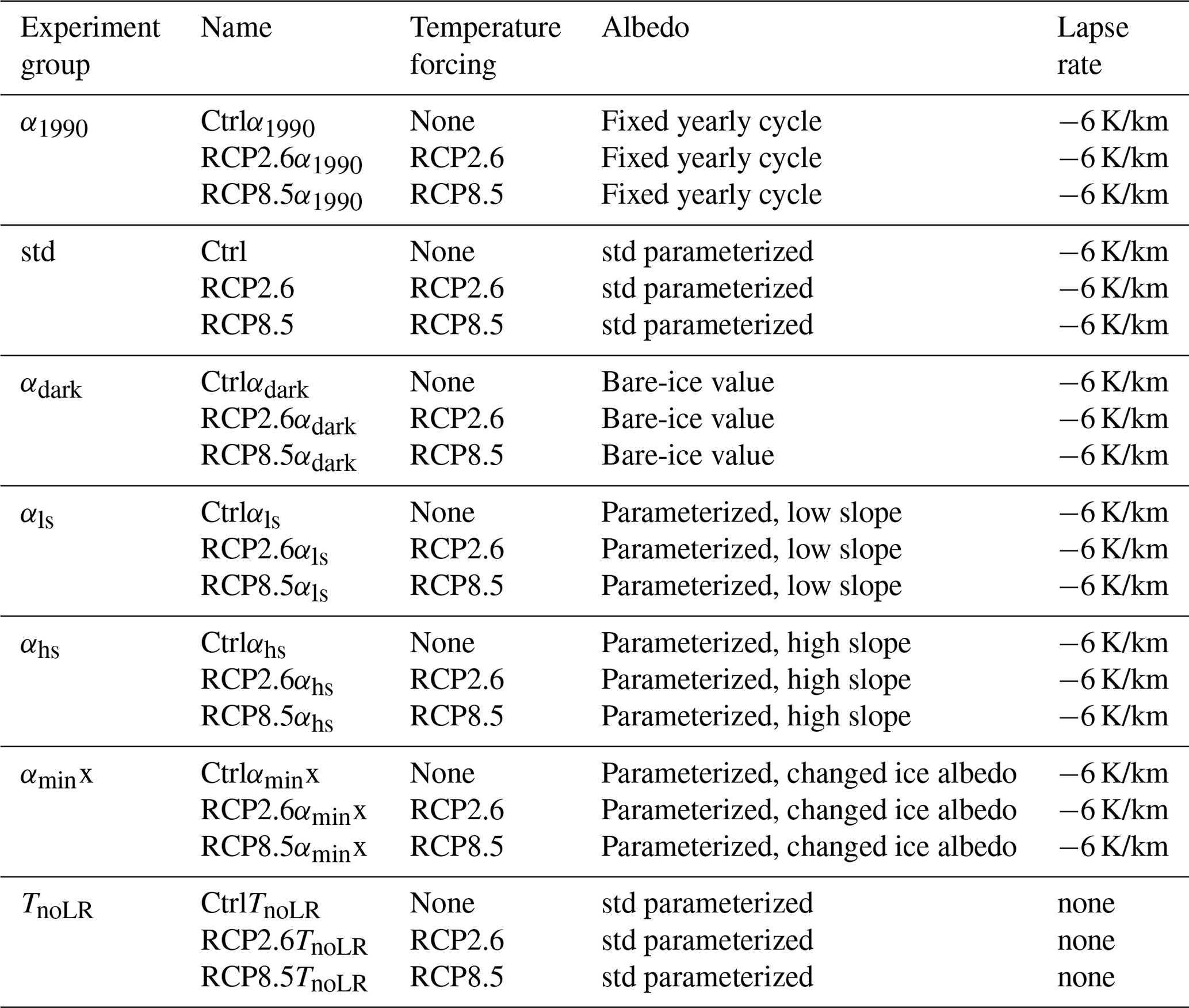
The experiments can be summarized into seven groups. The α1990 experiments use an interannually constant yearly albedo cycle and therefore suppress the adaptation of albedo to increased melt rates under warming. They are used to estimate future ice loss without the melt–albedo feedback and serve as a reference. The std experiments include the melt–albedo feedback through the standard parametrization for albedo. The αdark experiments represent an extreme scenario, assuming that the whole ice surface will be snow free or covered with meltwater during the months June, July, and August in each year. This is not a realistic scenario but rather an upper limit to the possible impact of albedo changes on ice loss. The αls, αhs, and αmin experiments explore the uncertainty from the albedo parametrization. Doubling the slope to −0.05 yr/m leads to a steeper decrease in albedo with increasing melt rates, which is closer to the conditions in August (see Appendix Fig. A1). Assuming that in the future the melting period over the Greenland Ice Sheet is longer and therefore the conditions we observe in August might be more characteristic over the melting period justifies the exploration of the impact of an increased sensitivity in the αhs experiments. However, in this approach the minimal albedo for bare ice remains at 0.47 and is therefore reached with melt rates of 7 m/yr (instead of 14 m/yr in the standard parametrization). Halving the slope to −0.013 yr/m explores the lower boundary of albedo–melt sensitivity (see Fig. A1) in the αls experiments. In the αmin experiments, we test the influence of a reduced minimum albedo, as observed today in the dark zone of the Greenland Ice Sheet. The TnoLR experiments neglect the atmospheric temperature lapse rate. Thus the local temperature is independent of the ice sheet topography, and the representation of the melt–elevation feedback is interrupted.
An overview of all experiments is given in Table 1.
In this section, we validate the dEBM-simple melt for present-day conditions and show as an example melt rates with Eemian insolation. The experiments are performed as described in Sect. 2.5.
3.1 Present-day melt rates
Here, we compare the melt modelled with PISM-dEBM-simple over the historic period with melt modelled by MARv3.11 (see Fig. 1). The setup is described in Sect. 2.5. Note that here the evolution of the ice sheet topography is suppressed; that is the melt rates are calculated over a fixed geometry corresponding to present day.
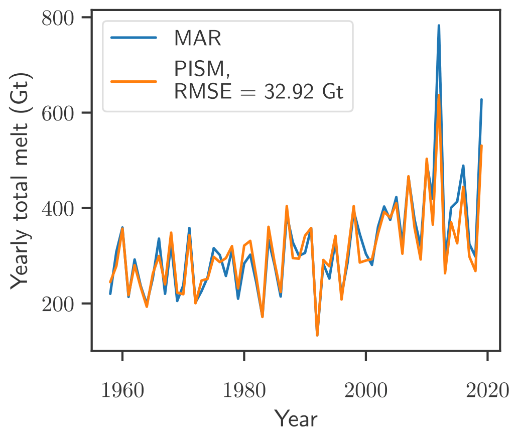
Figure 1Comparison of annual total melt of the Greenland Ice Sheet as calculated with MAR v3.11 and PISM-dEBM-simple. The diagnostic simulation with PISM-dEBM-simple (orange line) is performed using monthly MAR 2D temperature fields as forcing. The albedo αs is parameterized with the local melt rate m as , and the shortwave downward radiation is approximated by the top-of-the-atmosphere radiation and the transmissivity τA parameterized with surface altitude z as . The root-mean-square difference between the PISM-dEBM-simple simulation and total melt as given by MAR (blue line) is 32.92 Gt.
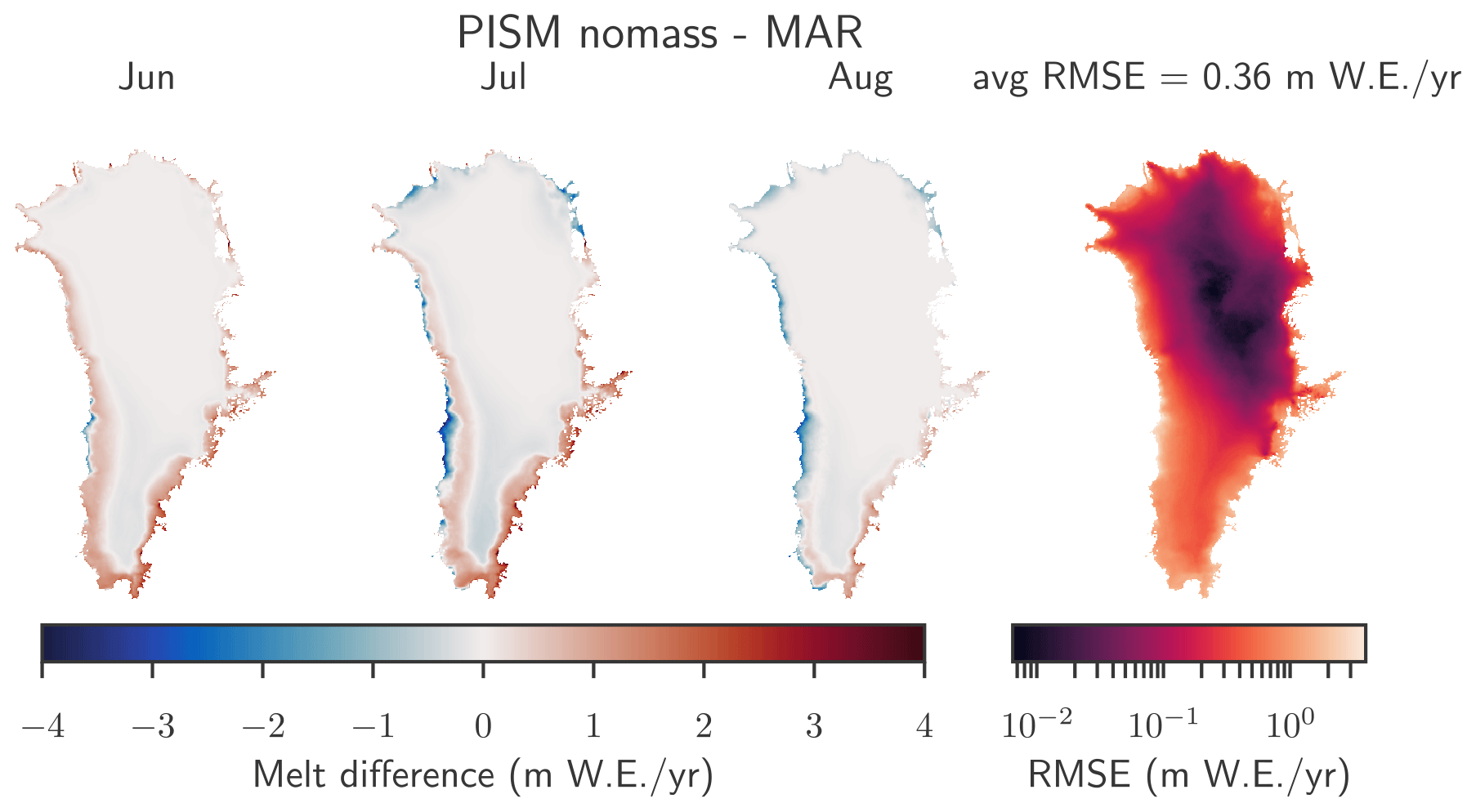
Figure 2Local differences between the monthly averaged June, July, and August melt rates as diagnosed with PISM-dEBM-simple compared to MAR. The PISM simulation uses monthly 2D temperature fields from MAR as forcing and parameterizes albedo and shortwave downward radiation as detailed in Sect. 2.3.1 and 2.3.2. Positive numbers mean that PISM overestimates the melt, and negative numbers mean that PISM underestimates the melt. The local root-mean-square error averaged over June, July, and August from 1958–2019 is shown in the right plot. The spatial average of the RMSE is 0.36 m/yr.
Due to the parametrization of the albedo and the transmissivity (and thus the shortwave downward radiation) detailed in Sect. 2.3 and in Table A2, the parameters of the dEBM-simple model are adjusted from Krebs-Kanzow et al. (2018). The chosen dEBM-simple parameters c1 and c2 (see Table A2) minimize the product of spatial and temporal root-mean-square error in the melt rate over the whole period from 1958 to 2019 while using the parameterizations for albedo and shortwave downward radiation. The temporal root-mean-square error is computed from a comparison of total yearly melt (see Fig. 1), and the spatial root-mean-square error is computed from a comparison of the 2D fields of summer (JJA) melt rates averaged over the whole period (see Fig. 2), both with respect to MAR data. Both of the root-mean-square errors are minimized by the dEBM-simple parameters c1 and c2 given in Table A2.
Yearly total melt computed with PISM-dEBM-simple follows the MAR data closely (see Fig. 1). That extreme melt years such as 2012 and 2019 are underestimated can be explained by the parametrization of shortwave downward radiation, which neglects temporal variability in the cloud cover, one of the drivers of recent mass loss in Greenland (Hanna et al., 2014; Hofer et al., 2017). We also test dEBM-simple with shortwave downward radiation and albedo from MAR directly. Figure A4 shows that in this case the extreme melt in 2019 is better captured, while melting in 2012 is still underestimated.
As Fig. 2 shows, melt is generally overestimated in June, at the beginning of the melt season, and underestimated as the melt season progresses. In July dEBM-simple underestimates melt mostly at the western margin, where ablation is highest. In August, toward the end of the melt season, melt is systematically underestimated by the dEBM-simple module, in particular in the regions where the darkest albedo values are observed. The systematic underestimation could be caused by taking a constant minimal value for the ice albedo and not allowing for processes which would lead to a natural darkening of the surface, i.e. algae growths, supra-glacial lakes, or ageing of snow or exposed ice. On the other hand, many of those processes, in particular bio–albedo feedbacks or dust deposition, are not yet represented in the MAR model either and thus should not induce a systematic bias when comparing to MAR data.
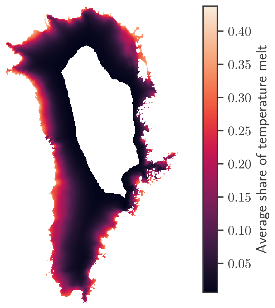
Figure 3Share of temperature-induced melt. The fraction of temperature-induced melt, defined as , is diagnosed with PISM-dEBM-simple and averaged over the months June, July, and August over the whole simulation period from 1958–2019. The white part in the centre illustrates areas of the Greenland Ice Sheet where the average melt is zero at present.
The melt Eq. (1) can be used to attribute the melt rates of the present day to temperature- or insolation-driven melt in a first-order approximation. To this end we compare both contributions to the total melt rate, with the temperature-driven melt and the insolation-driven melt . The share is then defined by over the regions which experience melt. Under present-day conditions, this approach indicates that the melt over the whole ice sheet is mainly driven by the insolation (see Fig. 3). Even at the margins, where monthly mean temperatures and the fraction of temperature-driven melt are highest, the fraction does not exceed one-half. In particular over the high and cold regions of the ice sheet, the melt seems to be entirely driven by the insolation, with an indirect effect of the temperature only allowing melt if monthly mean air temperatures are above −6.5 ∘C.
The model is able to capture melt patterns of the Greenland Ice Sheet over the historic period between 1958–2019 with a root-mean-square error of 32.92 Gt for the yearly total melt and an average root-mean-square error of 0.36 m w.e./yr for the local summer melt rates. A more thorough discussion on the performance and the sensitivity of the melt Eq. (1) (without the parametrization of albedo and transmissivity) and a comparison to the positive-degree-day model can also be found in Krebs-Kanzow et al. (2018). An overview of the performance of the full dEBM model compared with other state-of-the-art models can be found in Fettweis et al. (2020).
Overall, the skill of the PISM-dEBM-simple model under present-day conditions and using high-resolution forcing from MAR is similar to the skill of the full dEBM model (Krebs-Kanzow et al., 2021). Compared to MAR, dEBM revealed a RMSE of 27 Gt for the annual mean 1979–2016 climatic mass balance in an experiment which was forced with reanalysis data (Uta Krebs-Kanzow, personal communication, 2021). The dEBM full model accounts for changes in the atmospheric emissivity and transmissivity, both caused by changes in cloud cover. As the cloud cover was the main driver in the 2012 melt event, the full dEBM model is therefore better suited to reproduce this and similar melt events. Furthermore, dEBM computes the refreezing on the basis of the surface energy balance.
3.2 Sensitivity to Eemian solar radiation
The dEBM approach together with the approximations for albedo and transmissivity allows us to include changing orbital parameters for simulations on paleo timescales. Here we explore the melt response to Eemian (125 kyr before present) orbital parameters in order to test for the sensitivity to insolation values and compare with other results from the literature. Therefore we use the eccentricity e=0.0400, the obliquity , and the longitude of the perihelion . The insolation at the top of the atmosphere is then calculated as detailed in Sect. A1. We use the present-day topography for the diagnosis of melt rates and keep the surface air temperature fields unchanged from the previous experiment (MAR v3.11 in the period of 1958–2019).
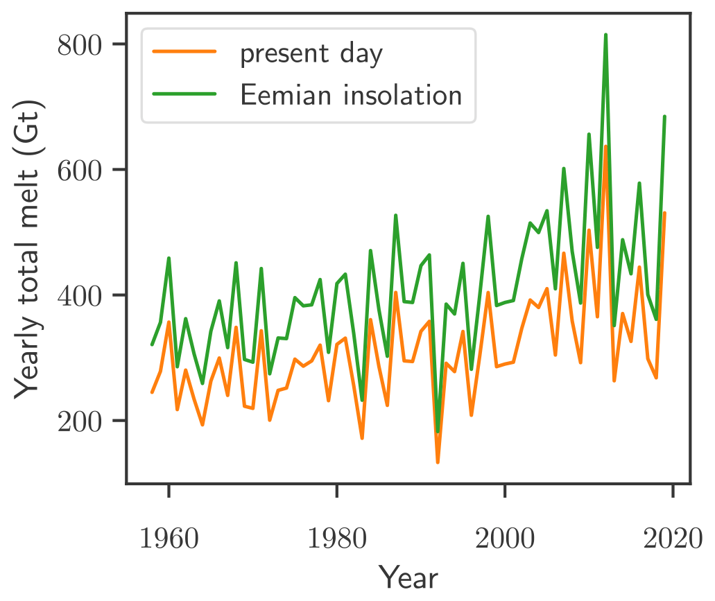
Figure 4Comparison of Eemian vs. present-day insolation in dEBM-simple. Yearly total melt of the Greenland Ice Sheet as diagnosed with PISM-dEBM-simple under present-day insolation (orange) and Eemian insolation (green). The diagnostic simulations with PISM were performed using monthly MAR 2D temperature fields as forcing and the parameterizations for shortwave downward radiation and albedo mentioned in the text.
The increase in solar radiation leads to increased melt, as seen in Fig. 4. The inter-annual variability in yearly total melt is very close to the present-day variability computed with MAR, mainly driven by inter-annual temperature changes. Averaged over the whole time period (1958–2019), the yearly total melt increases by 98 Gt/yr, which corresponds to a relative increase of 31 %. This is in line with findings of Van De Berg et al. (2011), who find that Eemian insolation alone leads to a 40 Gt/yr increase in runoff compared to present day and a 113 Gt/yr increase in runoff when compared to preindustrial values.
Here, we analyse how changes in albedo may impact the melt rates and the ice loss of the Greenland Ice Sheet under the greenhouse gas emission scenarios RCP2.6 and RCP8.5. In particular we focus on the melt–albedo feedback, and on the additional ice loss driven by changes in albedo. The experiments are motivated and described in detail in Sect. 2.6. The volume of the ice sheet and the mass losses until the years 2100 and 2300 due to the respective warming scenarios are summarized in Table 2.
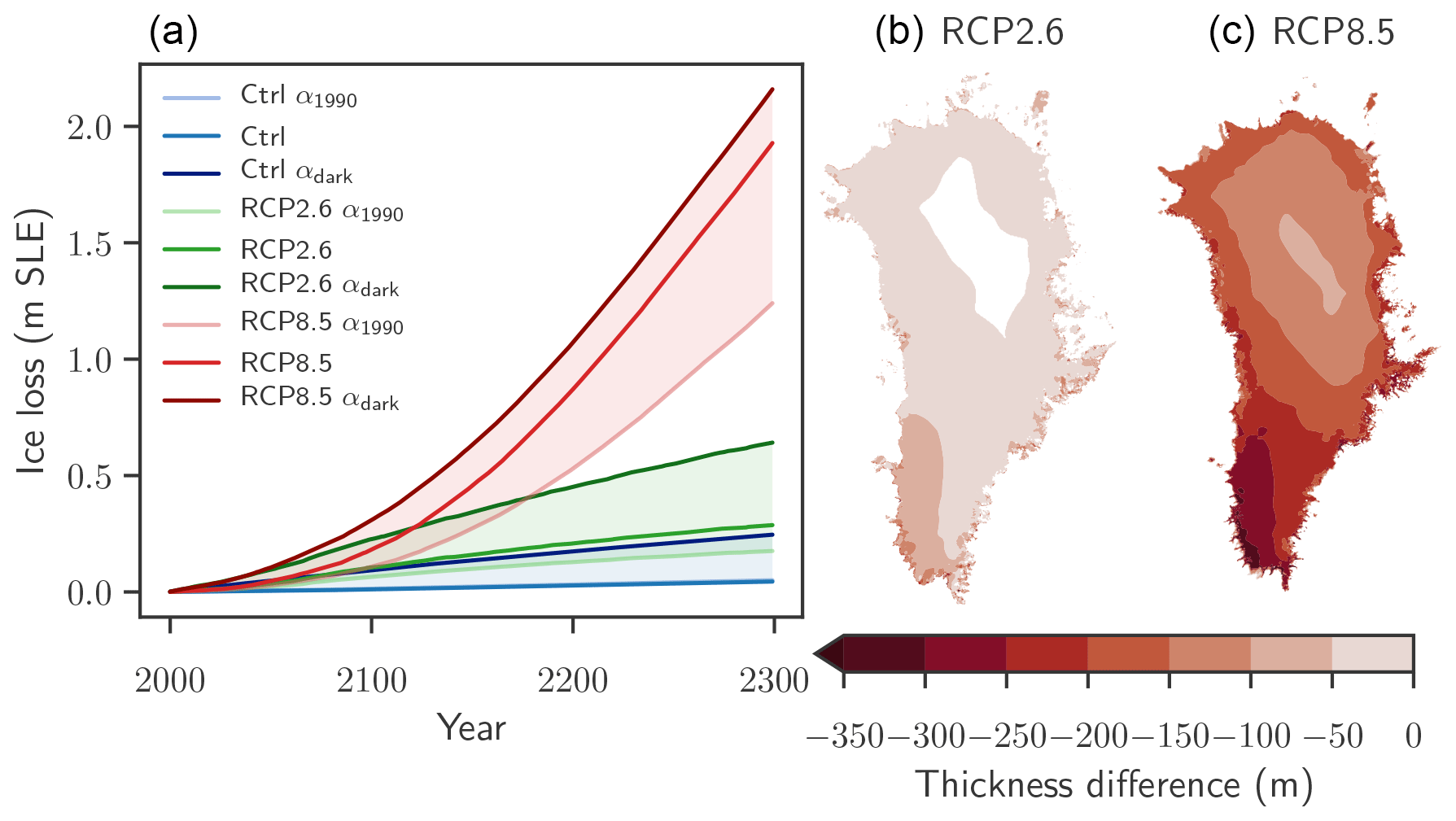
Figure 5Influence of the melt–albedo feedback on Greenland's ice loss under future warming. The scenarios consist of a control experiment (blue) and temperature forcing with RCP2.6 (green) and RCP8.5 (red). (a) Ctrl, RCP2.6, and RCP8.5: ice losses between 2000 and 2300 modelled with PISM-dEBM-simple using the standard parameters and the respective temperature forcing. α1990: ice losses for the respective temperature forcing with monthly albedo fixed to the average pre-1990 values, thereby interrupting the melt–albedo feedback. αdark: ice losses with the respective temperature forcing with summer albedos (June, July, August) set to the bare-ice value over the whole ice sheet. This yields an upper limit of ice loss driven by albedo changes. The shading is to illustrate the range between the lower and upper limits. Ice loss is given in metres of sea level equivalent. A value of 1 m s.l.e. corresponds to approx. 361 800 Gt of ice. Panels (b) and (c) show the ice thickness difference between the lower bound experiments α1990 and the standard experiments for RCP2.6 (b) and RCP8.5 (c) in the year 2300.

Figure 6Uncertainty of albedo-change-driven ice loss. Ice losses of the Greenland Ice Sheet under the Ctrl, RCP2.6, and RCP8.5 scenarios, exploring the effect of different albedo sensitivities, as described in detail in Sect. 2.3.2 and Fig. A1. Shaded regions correspond to the range between the lower and upper bounds for ice loss, as shown in Fig. 5. (a) Ice losses with variations in the minimal value for albedo. Lower αmin corresponds to darker bare ice. (b) Ice losses with variation in the slope of the albedo parametrization. αls experiments use a lower slope (half of the standard value); thus the sensitivity of albedo to melt is reduced. αhs experiments use a higher slope (double the standard value), thus increasing the sensitivity of albedo to melt. Ice loss is given in metres of sea level equivalent. A value of 1 m s.l.e. corresponds to approx. 361 800 Gt of ice.
Table 2Sea-level-relevant volume (in metres of sea level rise equivalent) and mass loss (in centimetres of sea level rise equivalent). All values are relative to the respective control simulation. Only αdark simulations are given in absolute values, since the Ctrl αdark is an extreme scenario which does not qualify as a control experiment.

4.1 Ice loss under warming without the melt–albedo feedback
The α1990 experiments use fixed monthly albedo fields and thereby interrupt the melt–albedo feedback. Those experiments illustrate a lower bound of ice losses due to warming in this model setup. Note that the lower bound of projected future ice loss under global warming likely differs due to the coarse resolution and the lack of ice–ocean interaction in this study. As described in Sect. 2.6, the monthly albedo in the α1990 experiments is fixed to an average yearly cycle given by the pre-1990 values in MARv.3.11. Consequently the insolation-related melt, as given by the first term of Eq. (1), remains constant or even decreases due to decreasing transmissivity of the atmosphere, and only the temperature-dependent term increases due to the warming.
In this scenario, the Ctrl α1990 experiment remains constant in volume, while the RCP2.6 α1990 shows 5.2 cm ice loss until 2100 and 12.6 cm until 2300. In the RCP8.5 α1990 experiment the ice loss amounts to 9.8 cm until 2100 and to 119 cm until 2300 (see Fig. 5). The mass loss until 2100 is in line with the estimate of 9±5 cm in the community-wide ISMIP6 projections (Goelzer et al., 2020). Note that in contrast to ISMIP6, the ocean-driven melting remains constant, even under increased temperatures, and there is no glacier retreat due to ice–ocean interactions. However, the mitigating effect of precipitation increase in a warmer climate is also missing.
4.2 Increased ice loss through the melt–albedo feedback
In the following we present the results for the std experiments with PISM-dEBM-simple, taking into account the melt–albedo feedback through the melt-dependent albedo parameterizations as described in Sect. 2. In the control simulation Ctrl, without temperature forcing or artificial darkening, the ice sheet is stable in volume on the timescale of 300 years.
In the RCP2.6 simulations, the moderate increase in temperatures leads to an approximately linear decline in ice volume with an ice loss of 9.4 cm until 2100 and 24.3 cm until 2300 in comparison to the year 2000. This is an increase in ice loss of +82 % in 2100 and +93 % in 2300 in comparison to the α1990 simulation without melt–albedo feedback; see Fig. 5 and Table 2. The RCP8.5 simulations show a strong and non-linear decline in ice volume, with ice loss of 16.8 cm in 2100 and 1.88 m in 2300. This corresponds to a relative increase of +80 % and +58 % respectively due to the melt–albedo feedback. The relative contribution of the melt–albedo feedback to ice loss keeps increasing with time for the RCP2.6 experiment, while it becomes less important with time for the RCP8.5 experiment, as the whole ice sheet approaches the minimal albedo value αmin. However, in absolute terms the melt–albedo feedback still contributes almost 70 cm s.l.e. mass loss in the RCP8.5 experiment until the year 2300.
We compare these values with the influence of the melt–elevation feedback (TnoLR; see Fig. C1). This feedback is weaker; it increases the ice loss by 18 % and 13 % in the RCP2.6 and RCP8.5 simulations respectively.
The melt–albedo feedback is particularly important in the south of Greenland, where the insolation averaged over the daily melt period (see Eq. 1) is highest. Until the year 2300 it initiates up to 100 m of additional thinning in the southwest for the RCP2.6 scenario compared to RCP2.6 α1990 (Fig. 5b). In the RCP8.5 experiment, the melt–albedo feedback is impacting the thinning over the whole ice sheet (Fig. 5c). However, the most important contribution remains in the southwest of Greenland, with an additional 300 m of thinning compared to RCP8.5 α1990.
4.3 An upper limit for ice loss through extreme surface darkening
As a next step, the upper limit of the melt–albedo feedback is explored via prescribing summer albedos equal to the bare-ice albedo over the whole ice sheet in each year (see details in Sect. 2.6). First, the effect of such a surface darkening is explored without any temperature forcing in the Ctrl αdark scenario. In this experiment approximately linear mass loss is observed, with a rate of 8 mm s.l.e. per decade (see Fig. 5a), and induces ice loss of 8.3 cm until 2100 and 20.1 cm until 2300. The condition that the local monthly mean air temperature needs to be higher than −6.5 ∘C to allow melt, prevents further melting in the ice sheet's interior. Topographic changes together with the temperature–lapse rate feedback increase the melt area slowly, but do not have a major impact over the 300 years. Note that this extreme darkening Ctrl αdark scenario alone induces more ice loss than the RPC2.6 α1990 scenario (see Fig. 5 and Table 2).
The RCP2.6 αdark experiment combines the extreme summer darkening with the RCP2.6 temperature anomaly, thereby increasing ice loss from the RCP2.6 α1990 experiment by more than a factor of 4 in comparison to the α1990 experiments (Fig. 5 and Table 2). This corresponds to a more than 4-fold increase in ice loss. The darkening together with the moderate temperature increase induces an expansion of the melt zone and thus strong melt in areas that are not affected in the Ctrl or RCP2.6 experiments. The ice volume evolution in the RCP2.6 experiment is closer to the lower than to the upper bound of the melt–albedo feedback.
In the RCP8.5 αdark experiment the summer darkening leads to an increase in ice loss of 214 % in 2100 and 77 % in 2300 in comparison to the no-feedback RCP8.5 α1990 experiment (see Fig. 5 and Table 2). The strong shock of albedo darkening is particularly relevant when overall temperature increases are still low. In contrast to the RCP2.6 αdark experiment, where the additional mass losses increase with time, here the relative impact of extreme summer darkening decreases on long timescales. As the warming progresses, the temperature becomes a more important driver to melt.
Reducing the frequency of darkening in the RCP2.6 αdark and RCP8.5 αdark experiments to darkening events every 2 or every 5 years instead of every year reduces the difference in mass loss between the RCP αdark and the RCP experiments (see Appendix Fig. B1). When the darkening happens every 2 years, the additional ice loss decreases to approximately half of the ice loss due to darkening every year. Similarly, a darkening event every 5 years leads to only 20 % of the additional ice loss due to the darkening in each year. The effect is approximately linear in event frequency. This might help to estimate additional albedo-driven ice loss in extreme years such as 2012, if projections for the frequency of such extreme events are available.
Reducing the length of the dark period from the whole summer (i.e. June, July, and August) to only 1 month reveals that the month of June is most sensitive to additional darkening, inducing more than half of the additional ice loss between the RCP8.5 and the RCP8.5 αdark experiments (see Appendix Fig. B1). The increased sensitivity to darkening in June could be due to the fact that the Northern Hemisphere receives the most insolation during the month of June. Moreover, in the beginning of the melt season the albedo has not yet decreased due to the melt processes, so an artificial darkening has the strongest effect, compared to the following summer months.
4.4 Exploring uncertainty in albedo-change-driven ice loss
The standard parameters for the albedo parametrization used in the RCP2.5 and the RCP8.5 experiments provide the best fit to the MARv3.11 data over the historic period. However, the range for possible contributions of the melt–albedo feedback is large; therefore we test how changes in the albedo parametrization affect the ice loss driven by albedo changes. The albedo parametrization can affect the strength of the melt–albedo in two ways: first by changing αmin, the lowest albedo possible, and second by changing the sensitivity of albedo to melt via the slope in Eq. (7). To ensure that the subsequent mass changes are not primarily due to model drift, they are corrected by a Ctrl experiment without warming but with otherwise identical parameters.
A decreased value of αmin does not affect regions where melt rates are below 14 m/yr. Consequently, strong melt rates are necessary to observe its impacts: in the RCP8.5 αmin simulations with αmin=0.4 the lowered αmin value causes an additional 5.3 cm of ice loss in 2300 (compared to RCP8.5), and the RCP8.5 αmin simulations with αmin=0.3, it causes an additional 16 cm until 2300 (Fig. 6a).
In contrast to the αmin experiments, changing the slope in the albedo parametrization in Eq. (7) affects the sensitivity of the albedo to melt already at low melt rates. In the Ctrl αhs experiment, the ice sheet loses 10 cm s.l.e. until 2300 from the increase in the albedo sensitivity alone, twice as much as with standard parameters. The increased melt sensitivity, although at the upper end of the uncertainty of the parameters presented in Sect. 2.5, might not be optimal in representing historical melt when the other parameters remain unchanged. We thus test the mass losses of the warming scenarios with respect to the Ctrl αhs experiment, in order to explore the interplay of an increased melt–albedo feedback and warming.
The additional effect of the increased sensitivity on ice volume evolution depends on the warming scenario. The RCP2.6 αhs experiment with moderate warming is affected by a more sensitive albedo parametrization, with up to 40 % increases in ice loss until 2300 with respect to the RCP2.6 experiment (see Fig. 6). In contrast, the additional mass loss in RCP8.5 αhs is lower with +6 % in 2300 compared to the RCP8.5 scenario. This can be explained by the fact that the high melt rates in the RCP8.5 scenario quickly induce the minimal albedo over the whole ice sheet and thereby interrupt the feedback. Once the minimal albedo is reached, further increase in melt rates does not affect the albedo any more; thus the melt is not affected by the stronger feedback any more.
If the sensitivity of albedo to melt is reduced, the ice sheet in the Ctrl αls experiment shows slight mass gains (4 cm over 300 years). The lower sensitivity mitigates mass losses from both the RCP2.6 αls and RCP8.5 αls experiments, with 8.3 and 29.4 cm less mass loss until 2300 respectively. However, even with the reduced melt–albedo feedback the ice loss increases by approximately one-third when compared to the α1990 experiment without albedo–melt feedback.
We have presented an implementation of a simple version of the diurnal energy balance model (dEBM-simple) as a module in the Parallel Ice Sheet Model (PISM). Using this model we evaluate how changes in albedo impact future mass loss of the Greenland Ice Sheet under the RCP2.6 and RCP8.5 warming scenarios.
5.1 Implementation and validation
In dEBM, the surface melt is calculated as a function of near-surface air temperature and shortwave downward radiation. A first version of the dEBM was tested and validated in Krebs-Kanzow et al. (2018), and a full version was presented in Krebs-Kanzow et al. (2021). dEBM-simple adapts the approach taken in Krebs-Kanzow et al. (2018) and adds additional modules to calculate the albedo as a function of melt and the shortwave downward radiation. Therefore, the only inputs needed to compute the melt rate are two-dimensional near-surface temperature fields including the yearly cycle and a precipitation field in order to close the climatic mass balance. This approach makes the model as input-friendly as a temperature-index model such as the widely used positive-degree-day model, but with the advantage of capturing the melt–albedo feedback. The dEBM-simple surface mass balance module can be used with PISM in a stand-alone setting to simulate past and future ice sheet evolution, requiring only a temperature field, a precipitation field, and the time series of the temperature anomaly as inputs. As PISM is an open-source project, the module can easily be expanded or implemented in other stand-alone ice sheet models.
Being a simple model, dEBM-simple does not fully resolve the spatial pattern and temporal evolution of melt over the Greenland Ice Sheet; the melt rates are slightly overestimated towards the beginning of the melt season (June) and underestimated towards the end of the melt season (August) and at the margins of the ice sheet. This is possibly related to the albedo parametrization, which underestimates the albedo in June and overestimates the albedo in August, not capturing important processes like exposure of firn or ice, or darkening of the ice via algae or meltwater. However, the total yearly melt rates match those of MAR over the period 1958–2019 well and on this timescale the skill of the model is comparable to the dEBM (Krebs-Kanzow et al., 2021). The exceptions of the extreme melt in the years 2012 and 2019, where dEBM-simple clearly underestimates melt rates, are related to changes in cloud cover or blocking events (Delhasse et al., 2021; Hanna et al., 2014; Hofer et al., 2017), which are not captured by the parametrization of the transmissivity of the atmosphere.
Increased insolation values like during the Eemian increase the melt on average by 97 Gt/yr under otherwise identical conditions. This is in line with the findings of Van De Berg et al. (2011). While this is only an approximation with several strong assumptions (e.g. the present-day topography of the ice sheet is preserved and we did not apply changes in the temperature), it illustrates the possibility of extending this model to paleo timescales with relatively low effort.
The implemented parametrization for albedo is based on a phenomenological relation of albedo to the melt rate. It is a coarse representation of the effects that are important for the snow albedo, such as the grain size, surface water and melt ponds, impurities (e.g. black carbon or algae), or any dependence on the spectral angle or the cloudiness condition of the sky. The possible darkening of ice is considered only indirectly in this approach. In particular, lowering the minimal allowed albedo to values which are typical for either dirty ice or supraglacial melt ponds could allow us to include an approximation of albedo changes of the bare ice itself. Moreover, the parametrization neglects the impact of the snow cover thickness, which might mitigate melt-driven reduction in albedo after a winter with heavy precipitation (Box et al., 2012). As the parameters of the albedo scheme are fitted against monthly averages of the MAR albedo, processes which happen on a sub-monthly timescale are not well captured. The ageing or renewal of snow, associated with the frequency of snowfall events, is not directly represented in the monthly averaged MAR data used to fit the parameterization. Neither is the influence of shading, wind exposure, or rain spells. These could induce additional variability associated with the albedo–melt relations.
Similarly, the parametrization introduced for the shortwave downward radiation does not take into account temporal or spatial patterns. The inter-annual variability of the cloudiness over Greenland and blocking events can therefore not be represented with this approach.
However, the introduced parameterizations do not introduce a systematic bias or a large additional error in comparison to a purely diagnostic mode of dEBM-simple, where instead of parameterized albedo and shortwave downward radiation the 2D fields of MAR output are used to calculate the melt rates (see Fig. A4), while all other parameters are kept constant.
In this paper we optimize the dEBM parameters c1 and c2 independently from the parameters for the albedo and the transmissivity. All parameters are based on MAR v3.11 data. While this procedure gives an overall good fit, as seen in Sect. 2.5, it is not necessarily the optimal solution in combination. However, this procedure keeps the parameters independent from the forcing. One could, based on the application, choose to change the parameterizations independently from the dEBM parameters and thereby study the influence on the ice loss, as we have shown in Sect. 4.4.
In comparison to the widely used positive-degree-day model, PISM-dEBM-simple performs slightly better for both measures: the monthly averaged spatial melt and the integrated yearly melt (see Appendix D).
5.2 Sensitivity of the Greenland Ice Sheet to warming and surface darkening
In this paper we use the PISM-dEBM-simple model in order to assess the influence of albedo changes and surface warming on the Greenland Ice Sheet. The simple surface mass balance model allows a first estimate of the influence of the melt–albedo feedback on the future evolution of the Greenland Ice Sheet in two temperature scenarios: moderate-warming RCP2.6, a scenario compatible with the Paris Agreement, and high-warming RCP8.5, a worst-case scenario. Experiments with a fixed yearly cycle of the albedo suppress the melt–albedo feedback and thus serve as a lower bound to future ice loss. In contrast, the extreme scenario in the αdark experiments with the surface albedo lowered to the bare-ice value over the whole ice sheet for the months June, July, and August serves as an upper bound for future melt through the melt–albedo feedback. The experiments with adaptive albedo serve as a more realistic estimate of future mass losses.
This experimental design allows us to attribute ice loss to the melt–albedo feedback. Overall we find that the melt–albedo feedback has a strong influence on melt under future warming. For example in the RCP2.6 scenario, the ice loss almost doubles through the albedo feedback (compare RCP2.6 with RCP2.6 α1990). Moreover, the relative amount of ice loss driven by changes in albedo keeps increasing over time. In contrast, the share of melt, driven by albedo changes, is lower in the high-temperature RCP8.5 scenario and decreases as the temperature increases, indicating that temperature is a more important driver under these conditions. Note, however, that the absolute increase in mass loss through the feedback is higher for RCP8.5 than for RCP2.6. We also find that extreme darkening alone, without any temperature anomaly, can initiate mass losses comparable to the RCP2.6 scenario.
Moreover, the interaction between the extreme darkening and warming initiates additional ice loss. In particular, the RCP2.6 αdark scenario loses 23 % more mass until 2300 than the sum of RCP2.6 and the Ctrl αdark simulations, suggesting that other feedbacks, such as the melt–elevation feedback, enhance the mass loss of the RCP2.6 αdark scenario.
An ensemble analysis over the ice loss in the RCP8.5 scenario reveals how sensitive the model is towards variations in the dEBM-simple albedo and transmissivity parameters (see Appendix E). All of the simulated ice loss remains within the bounds given by the α1990 and αdark experiments. Variations in the intercept of the atmospheric transmissivity have the greatest impact on ice loss, where higher values for the intercept shift the albedo- and insolation-dependent melt to higher values. Other parameters which seem to influence ice loss are the dEBM parameter c1, which governs the relation to temperature, and the slope of the albedo parametrization. Here, higher absolute values favour higher ice loss. On the other hand, the dEBM-simple parameter c2 and the slope of the transmissivity parametrization do not seem to have a strong effect on overall ice loss in a high-temperature scenario.
In this setup the melt–elevation feedback has a smaller impact on ice loss than the melt–albedo feedback: experiments which neglect the melt–elevation feedback (here parameterized through the atmospheric temperature lapse rate of −6 K/km) lose 18 % less mass in the RCP2.6 TnoLR scenario and 13 % less in the RCP8.5 TnoLR scenario until 2300 (see Fig. C1). This is in line with previous studies (Le clec'h et al., 2019) and suggests that the melt–elevation feedback, although weaker than the melt–albedo feedback, should not be neglected on the timescale of several centuries.
In comparing the ice loss with PISM-dEBM-simple in the RCP8.5 scenario to ice loss computed with PISM-PDD, we find that the positive-degree-day method increases losses by 12 % until 2100 and by 47 % by 2300 (see Appendix D). The losses for the RCP2.6 scenario do not differ significantly between PDD and dEBM-simple. The increase in ice loss for PDD can be explained by a higher temperature sensitivity of the PDD method: once all snow has melted, the sensitivity to positive-degree days (which is the time integral of Eq. 3) is given by the degree day factor for ice fi=8 mm/(K d). In contrast, with the parameters used in this paper, dEBM-simple scales to Teff only with ≈4.37 mm/K d (plugging in the constants in Eq. (1) and assuming , which is at the upper end of possible values). Thus, once the albedo effect saturates, PDD predicts higher melt rates with increasing temperatures. Moreover, due to the melt–elevation feedback, local temperatures rise even faster with increasing melt, leading to a stronger divergence between the dEBM-simple and the PDD ice loss.
In this study, we assume simplified representations of both the melt–elevation and the melt–albedo feedbacks. However, certain effects such as the feedbacks between the topography of the ice sheet and the atmospheric conditions which affect the surface mass balance cannot be expressed in the atmospheric temperature lapse rate alone. Similarly, the albedo is affected not only by melt, but also by the sky conditions, snow events, and impurities. While PISM-dEBM-simple is computationally efficient and represents the ice dynamics well, it cannot compete with an explicit process-based snowpack model as used by the regional climate models MAR or RACMO (Le clec'h et al., 2019; Kuipers Munneke et al., 2011) or represent the effect of summer snowfall on albedo (Noël et al., 2015). Moreover, here the melt–albedo feedback is represented by a relation linear at low melt rates and obtained from a MAR simulation over the historic period 1958–2019. This relation might not apply under future warming. Therefore we test uncertainties related to the albedo parametrization, with the resulting mass losses lying in the range between the lower bound, i.e. the no-feedback scenario, and the upper bound, i.e. the extreme-darkening scenario. Further analysis of the influence of the melt–albedo feedback with models that fully resolve the firn layer would be helpful to analyse processes that are neglected or simplified in this paper.
In observations, long-lasting albedo changes are already found as a consequence of heat waves which initiate strong surface melt (Nghiem et al., 2012; Tedesco and Fettweis, 2020). While the regions with the most rapid darkening in Greenland are located in the ablation zones, ice-sheet-wide melt events trigger albedo changes over the whole ice sheet (Tedesco et al., 2016). Studies suggest that heat waves in the Arctic may become more frequent with future warming (Dobricic et al., 2020), with still unknown consequences to ice sheet melt and albedo. Currently, there are no explicit albedo projections that take all processes and feedbacks like the distribution of surface meltwater, algae growths, dust deposition, and dust meltout into account. While PISM-dEBM-simple does not explicitly model all these processes, it adds a tool to explore albedo change scenarios and their influence on the future evolution of the ice sheet in a numerically efficient way, which takes the ice dynamics into account.
The module dEBM-simple is implemented in the open-source Parallel Ice Sheet Model (PISM) and captures albedo- and insolation-dependent melt as well as temperature-driven melt in stand-alone ice sheet simulations. Due to its simplicity, it can be used to perform large-scale ensemble studies or long-term simulations over centuries to millennia. The source code is fully accessible and documented, as we want to encourage improvements and implementation in ice sheet other models. This includes the adaption to other ice sheets than the Greenland Ice Sheet.
Using PISM-dEBM-simple we find that the melt–albedo feedback can lead to an additional 12 cm of sea level equivalent of mass loss in RCP2.6 and an additional 70 cm in RCP8.5 in the projected mass loss until the year 2300 with PISM. While our experiments rely on a simple parametrization of albedo with surface melt, they show that future albedo changes can make an important contribution to Greenland's future mass loss.
A1 Parametrization of albedo as a function of melt
Albedo is complicated to parametrize correctly, because of its dependence on a number of factors: the snow or firn albedo depends on grain size, impurities, surface water, refrozen ice, compaction, sky conditions, and spectral angle while the ice albedo depends on impurities, surface water, sky conditions, and spectral angle. Here we aim for a very simple phenomenological parametrization of albedo, which is good enough to be valid on large spatial scales and on long timescales. Only the broadband albedo is parameterized here, assuming that the average cloudiness of the sky does not change over long timescales. Further, it is assumed that grain size and surface water can be summarized in a single dependence of the albedo on the melt rate.
In the MAR v3.11 dataset, a negative correlation of albedo with melt is found (see Fig. A1). The average relation over the months June, July, and August in the period of 1958–2019 can be best described by the linear relation , indicated by the dashed orange lines in Fig. A1. The intersection with the y axis is interpreted as average snow albedo. At very high melt rates the albedo is less sensitive to additional increases with melt, which might be caused when the snow cover disappeared and bare ice is exposed. In this parametrization we introduce a lower limit to the albedo such that it can not be lower than 0.47 (approximately the value for bare ice Gardner and Sharp, 2010; Bøggild et al., 2010). This value is lower than the MAR value for bare ice, but in line with MODIS and RACMO at the ice margin, where impurities can accumulate (Noël et al., 2018; van Dalum et al., 2020; Stroeve et al., 2013). There is a large variance in how sensitively albedo is related to melt, which is due to both spatial and temporal (intra-annual as well as inter-annual) variability. However, a clear long-term trend of how the albedo depends on surface melt could not be established. In July, the albedo is on average less sensitive to melt, with an average slope of −0.021 yr/m. In June the monthly fit is identical to the whole summer, and in August the albedo decreases on average more strongly with melt, corresponding to a slope of −0.034 yr/m. In addition, in August there is a broad distribution of albedo values at zero melt, ranging from approximately 0.57 to the fresh snow value, which underlines that the correct albedo depends not only on the current condition but also on the melt during the past months. In order to estimate the sensitivity of future ice evolution to the exact parameters of the albedo parametrization, we vary the slope of the albedo over a broad range, by taking the double or half slope found with the linear regression, here indicated with the grey lines.
We tested other albedo parameterizations, which are successfully used in other models (e.g. Krebs-Kanzow et al., 2021; Krapp et al., 2017; Robinson et al., 2010).
We found that it is also better suited than a parametrization with the snow thickness, successfully used by many models as well (Krapp et al., 2017). The parametrization with snow thickness did lead to too low of albedo values and thus too high of melting in northwest Greenland, where precipitation is generally low. In our implementation, we found that the continuous relation of albedo to melt performed better to predict melt. Our approach comes with the caveat that the snow thickness is not considered for the calculation of the albedo, although observations suggest that increased winter snow can mitigate summer melt due to the higher albedo of the snow (Box et al., 2012; Riihelä et al., 2019).
The spatial distribution of summer albedos is shown in Fig. A2.
A2 Parametrization of shortwave downward radiation
Shortwave downward radiation that reaches the ice sheet's surface depends on the incoming radiation at the top of the atmosphere, the solar zenith angle, the surface altitude, and the cloud cover. In order to get the most correct estimate of shortwave downward radiation at the ice sheet's surface, it would be ideal to know the monthly average cloud cover. Since here we aim for a parametrization, which makes the model as simple as a temperature index model concerning the inputs needed, we instead parametrize the transmissivity of the atmosphere with the assumption that the average cloud cover does not change, either during the summer months or on longer timescales. Following Robinson et al. (2012), we assume that the transmissivity is solely a function of the surface altitude. In order to get a best estimate to this relation, the top of the atmosphere (TOA) radiation, which depends only on season and latitude, is compared to the MAR output for shortwave downward radiation. The daily average TOA radiation is described by Eq. (4). The local shortwave downward radiation SW would then be
A linear relation of the transmissivity to the surface altitude is given by
with the surface elevation in metres z and the fit parameters a and b. The linear fit for the shortwave downward radiation from TOA insolation was obtained from a linear regression of MAR v3.11 data averaged over June, July, and August from 1958 to 2019 (see Fig. A3).
Because melting occurs predominantly over the summer months June, July, and August, we derive the average transmissivity of the atmosphere based on the transmissivity calculated in MAR in June, July, and August. The best fit over these 3 months simultaneously is obtained with a=0.57 and b=0.037 km−1, as indicated by the orange dashed line in Fig. A3. A seasonality can be observed: the transmissivity is on average higher in June (a=0.61 and b=0.026 km−1) than in July (a=0.57 and b=0.040 km−1) and August (a=0.053 and b=0.046 km−1).
For simulations under paleo-conditions, changes in orbital parameters affect the insolation at the top of the atmosphere, and the trigonometric expansion used under present-day conditions (see Sect. 2.3.1) does not hold. The declination angle is then described by sin δ=sin (ϵ)sin (λ) and the sun–earth distance
with the oblique angle ϵ, the eccentricity e, the precession angle ω, and the true longitude of the earth λ. The orbital parameters e,ϵ, and ω are given in the input, while λ varies over the time of the year and is computed internally using an approximation of Berger (1978):
with
Here λ=0 at the spring equinox. This approximation is used only for explicit paleo simulations.
Liou (2002)Krebs-Kanzow et al. (2018)Krebs-Kanzow et al. (2018, 2021)
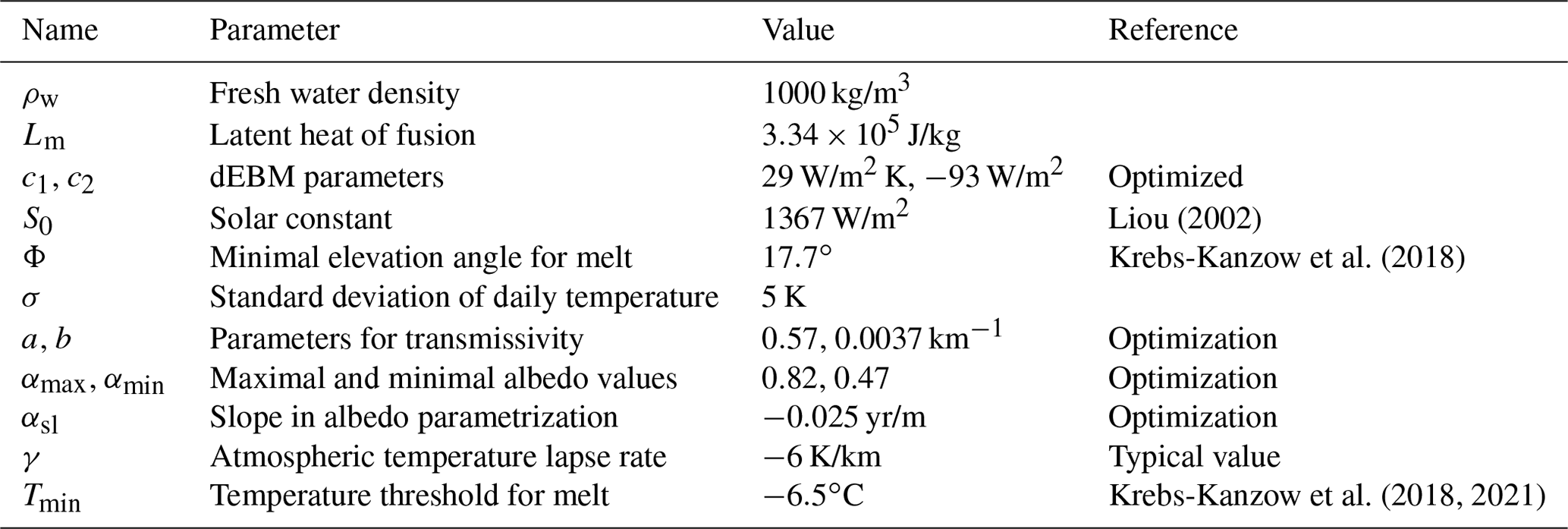
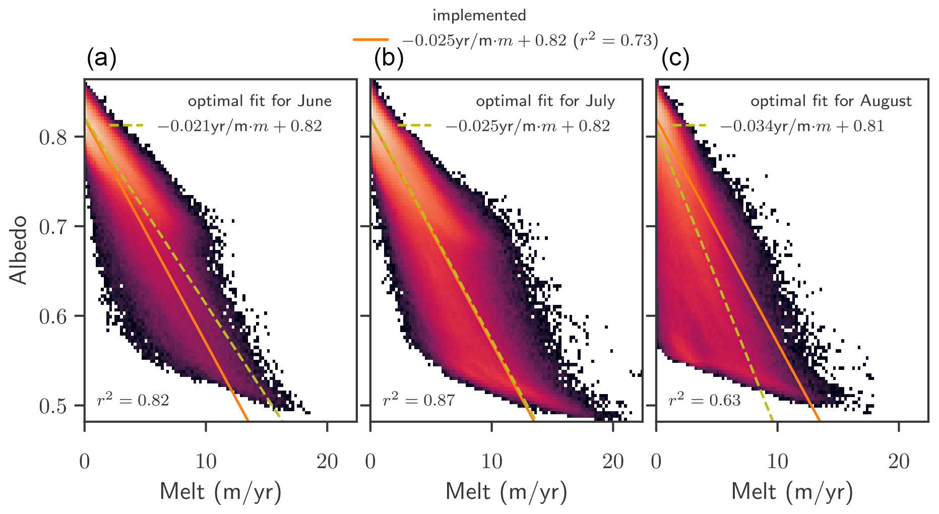
Figure A1Fit for albedo parametrization. Histograms of albedo vs. melt in June (a), July (b), and August (c) over the period 1958–2019 in the MAR v3.11 dataset. Colours represent how often the combination of values is found in each grid cell on the ice sheet over the years. Note that the colour scale is logarithmic. Orange lines show the parametrization with parameters as used in PISM. Light green lines show the best linear fit for each month, with the parameters given in the legend.
A3 Validation of parametrization
In order to assess the validity of the parameterizations in PISM-dEBM-simple, the yearly melt with the fully parameterized model, as shown in Fig. 1, is compared to the yearly melt of a diagnostic analysis of dEBM-simple with otherwise fixed parameters. Instead of computing the albedo and the shortwave downward radiation internally, monthly fields of those variables from the MAR v3.11 date are given as input to compute the melt rates via Eq. (1) with the same parameters c1 and c2. While the diagnostic experiment performs better in the extreme melt years 2012 and particularly 2019, we find an increased mismatch, in particular in the 1970s, and a resulting larger root-mean-square error. This can be attributed to the fact that the parameters c1 and c2 were optimized for a low temporal and spatial RMSE with the parameterizations for albedo and transmissivity as described above. c1 and c2 differ from Krebs-Kanzow et al. (2018) and from an optimal value for the diagnostic melt rate.

Figure A2Observed albedo. Local probability to find an albedo value within the given bracket on any day in June, July, or August from 2000–2019. Data: MODIS Greenland albedo; see Box et al. (2017).

Figure A3Fit for the parametrization of transmissivity. Shortwave downward radiation vs. surface altitude in June (a), July (b), and August (c) over the period 1958–2019 in the MAR v3.11 dataset. Each dot represents values in one cell of the ice sheet, averaged over a month. Orange lines show the parametrization with parameters as implemented, which is the best fit over the 3 months June, July, and August together. Light green lines show the best linear fit for each month, with the parameters given in the legend.
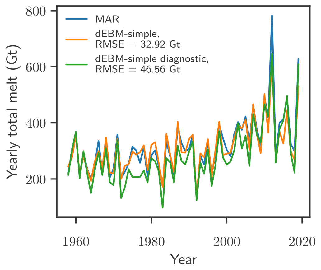
Figure A4Yearly total melt of the Greenland Ice Sheet as calculated with MAR (blue), diagnosed with the fully parameterized PISM-dEBM-simple simulation (orange), which uses only the monthly 2D temperature fields as input, and diagnosed with a non-parameterized diagnostic dEBM-simple version, which takes the 2D temperature field, the shortwave downward radiation, and the albedo as inputs. The root-mean-square error for the individual time series is given in the legend.
In order to test how the results are impacted by a shorter darkening period or even stronger albedo forcing, we study the upper-limit RCP8.5 αdark scenario in greater detail.
Shortening the darkening period to only 1 month reduces, as expected, the impact of darkening. Moreover, it reveals which months are the most vulnerable to darkening. In particular, we observe that darkening in June leads to the highest mass losses (see dashed–dotted line in Fig. B1a). Darkening in June alone leads to 9.6 cm of additional mass loss in 2100 and to 14.8 cm of additional mass loss in 2300 compared to the warming RCP8.5 scenario without darkening. In contrast, darkening in only July or August has a less significant effect, with 4.3 and 1.4 cm of additional mass loss in 2100 and 7.5 and 5.4 cm in 2300. On the one hand this might be caused by the larger insolation and longer days during the month of June. In June average daily insolation at latitudes above 60∘ N is approximately 7 % larger than in July and 50 % larger than in August. Moreover, due to the high melt in the warming RCP8.5 scenario, albedo values are already low in July and August, even without darkening.
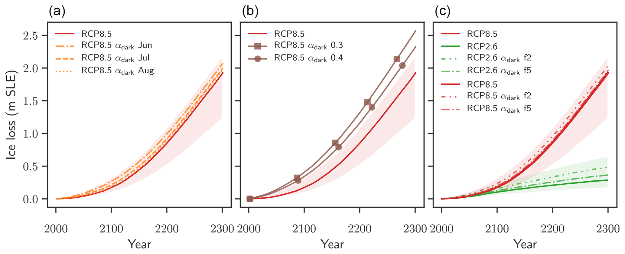
Figure B1Sensitivity to the darkening scenario. Ice volume evolution for different implementations of the darkening scenario. The envelopes of minimal and maximal mass loss, given by the α1990 and αdark experiments, and the RCP simulations with standard parameters are shown for reference. (a) Periods of extreme darkening in the αdark scenario are shortened to 1 month (orange broken lines). (b) The albedo value for extreme summer darkening is lowered to 0.3 (brown line with square markers) or 0.4 (brown line with circle markers). (c) Reducing the frequency of extreme darkening summers to every 2 (f2) and every 5 years (f5). Ice loss is given in metres of sea level equivalent. A value of 1 m s.l.e. corresponds to approx. 361 800 Gt of ice.
Using an albedo value which is lower than the value for bare ice leads to increased ice loss. An albedo value of 0.4 instead of 0.47 over the whole ice sheet increases ice loss by an additional 16 % or 4.6 cm by the year 2100 and by an additional 8 % or 17 cm by the year 2300 compared to the RCP8.5 αdark scenario. An even lower albedo value of 0.3 increases ice loss by an additional 37 % or 11 cm by 2100 and by an additional 19 % or 41 cm by 2300 compared to the RCP8.5 αdark scenario.
Reducing the frequency of dark summers to every 2 years leads to additional mass losses which are approximately half of the additional mass losses caused by the darkening in every year for both warming scenarios. A darkening frequency of every 5 years leads to additional mass losses of about 20 % of the additional mass loss with darkening in every year. This suggests that, at least on timescales of 300 years, the effects of more or less frequent darkening remain linear.
The melt–elevation feedback is generally represented in all experiments by adjusting surface temperatures with height changes by 6 K/km. The influence of the feedback on the simulations is tested by switching off this lapse-rate correction, with the resulting mass loss shown in Fig. C1.
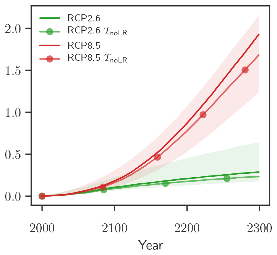
Figure C1Impact of the melt–elevation feedback. PISM-dEBM-simple simulations of the Greenland Ice Sheet with RCP2.6 (green lines) and RCP8.5 (red lines) warming. Dark solid lines take the melt–elevation feedback through the atmospheric temperature lapse rate into account. Shaded lines with markers neglect the melt–elevation feedback and assume a zero atmospheric temperature lapse rate. Ice loss is given in metres of sea level equivalent. A value of 1 m s.l.e. corresponds to approx. 361800 Gt of ice.
During the historic validation period, the simulation with the positive-degree-day method (PDD) for melt has a similar performance to PISM-dEBM-simple (see Fig. D1). The standard parameters were used for this simulation: the standard deviation of the temperature σ=5 K, the melt factor for ice fi=8 (mm liquid water equivalent) (pos degree day) and the melt factor for snow fs=3 (mm liquid water equivalent) (pos degree day). However, the spatial distribution of melt anomalies shows a distinct north–south gradient, with an overestimate of melt in the north and an underestimate of melt in the south; see Fig. D2.
In the warming simulations, the simulations with PDD melting show increased melt compared to dEBM-simple in the high-temperature scenario (see Fig. D3).
In RCP2.6 the north–south bias in the melt rates compared with PISM-dEBM-simple persists. However, the positive and negative biases balance each other out and lead to mass losses very similar to those computed with PISM-dEBM-simple. In contrast, the melt rates in the RCP8.5 scenario are almost consistently higher with the PDD melt module; only in the southwest does PISM-dEBM-simple produce higher melt rates than PDD. We find an increase in ice loss of 12 % in the year 2100 and of 47 % in 2300, compared to the standard dEBM run. The difference between ice loss computed with dEBM and with PDD is not only due to different sensitivities to temperature increase.

Figure D1Comparison of annual total melt of the Greenland Ice Sheet as calculated with MAR v3.11 and PISM-PDD. The diagnostic simulation with PISM-PDD (green line) is performed using monthly MAR 2D temperature fields as forcing. The root-mean-square difference between the PISM-PDD simulation and total melt as given by MAR (blue line) is 39.84 Gt. Details on the PISM-dEBM-simple simulation are found in Fig. 1 and in Sect. 3.
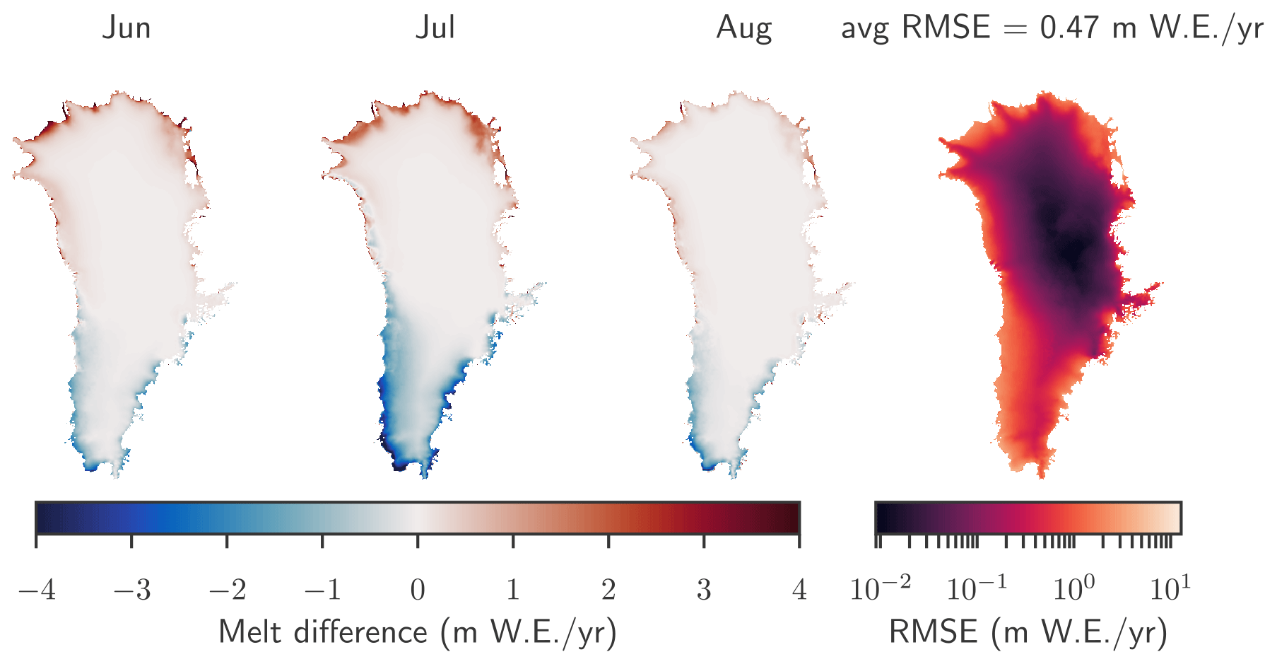
Figure D2Local differences between the monthly averaged June, July, and August melt rates as diagnosed with PISM-PDD compared to MAR. The PISM simulation uses monthly 2D temperature fields from MAR as forcing. Positive numbers mean that PISM overestimates the melt, and negative numbers mean that PISM underestimates the melt. The local root-mean-square error averaged over June, July, and August from 1958–2019 is shown in the right plot. The spatial average of the RMSE is 0.47 m/yr.
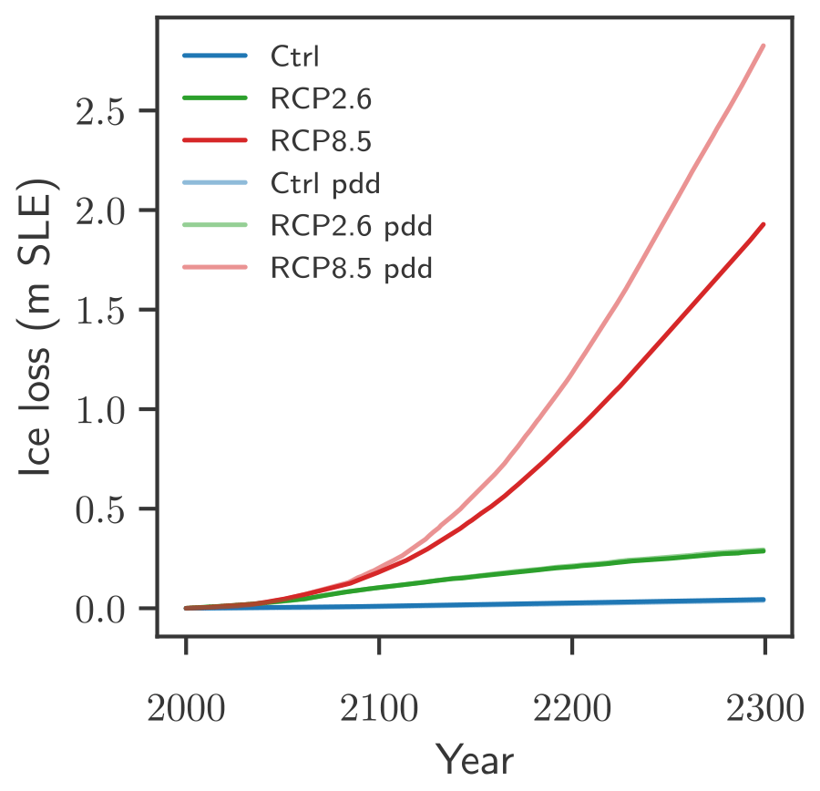
Figure D3Comparison with the positive-degree-day model. PISM-dEBM-simple and PISM-PDD simulations of the Greenland Ice Sheet with RCP2.6 (green lines) and RCP8.5 (red lines) warming. Ice loss is given in metres of sea level equivalent. A value of 1 m s.l.e. corresponds to approx. 361800 Gt of ice.
In addition to the RCP8.5 simulation with standard parameters, we tested how the variability of the parameters impacts the volume changes under an RCP8.5 forcing. Here, the experimental protocol is analogous to the protocol for standard parameters, described in the main paper in Sect. 2. However, instead of using only the standard set of parameters, the values for five parameters have been drawn randomly from a uniform distribution, creating an ensemble of 100 members. The varied parameters are summarized in Table E1.
The dEBM parameters c1 and c2 were derived by optimization of historic melt rates (see Sect. 3); therefore we do not have an estimate of a mean or a standard deviation. The range of parameters which were used for this ensemble were chosen such that for all parameters c1 and c2 the root-mean-squared error in the historic melt rates does not increase by more than 10% compared to the standard values. The parameters which describe the albedo and the transmissivity parameterizations were chosen such that the intra-annual variability is represented (see Appendix A).
The volume change of each ensemble member remains in the envelope given by the RCP8.5 α1990 simulations as a lower bound and the RCP8.5 αdark as an upper bound (see Fig. E1a). The variability of the intercept of the transmissivity parametrization has the largest influence on the variability in ice loss after 300 years due to warming. The ice loss until 2300 also seems to be correlated (or anti-correlated) to the dEBM parameter c1 and the slope of the albedo parametrization, while the dEBM parameter c2 and the slope of the transmissivity parametrization seem to have only negligible influence on the ice loss due to warming (see Fig. E1b–f).
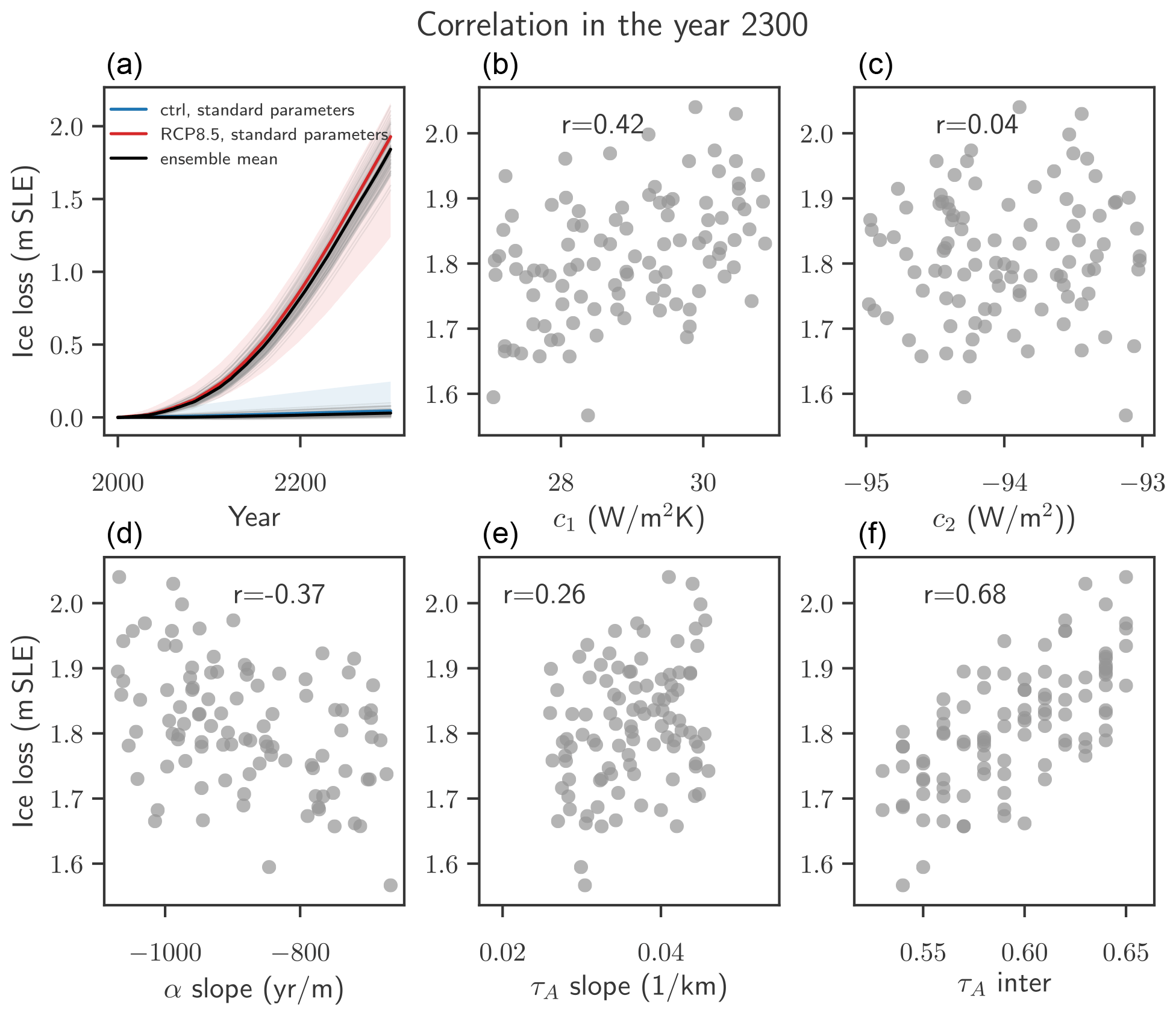
Figure E1Impact of the parameter variability. (a) Time series of PISM-dEBM-simple simulations of the Greenland Ice Sheet with RCP8.5 warming and control simulations. The thick red and blue line are simulations with standard parameters, and the shading shows the upper and the lower bounds of the melt–albedo feedback, as shown in Fig. 5 and discussed in Sect. 4. The thin black lines are the ensemble simulations, with parameters drawn in randomly and shown in Table E1. Thick black lines show the ensemble average. Ice loss is given in metres of sea level equivalent. A value of 1 m s.l.e. corresponds to approx. 361 800 Gt of ice. (b–f) Ice loss until the year 2300 in m s.l.e. vs. each of the varied parameters. Note that here the ice loss is corrected by the respective control simulation, which uses the same set of parameters but has no temperature forcing. The Spearman correlation coefficient is given in each of the panels.

The PISM source code including the dEBM-simple module is freely available through https://github.com/mariazeitz/pism/tree/pik/dEBM_dev (Zeitz, 2021). The code of the regional climate model MAR is available through https://mar.cnrs.fr/ (Drira, 2016). The CMIP5 datasets for the RCP2.6 and the RCP8.5 warming scenarios are available through https://esgf-node.llnl.gov/search/cmip5/ (Department of Energy, 2021).
The supplement related to this article is available online at: https://doi.org/10.5194/tc-15-5739-2021-supplement.
MZ implemented the dEBM-simple module with the parameterizations for albedo and shortwave downward radiation and performed the analysis. RW conceived the study. JB contributed the initial state for PISM simulations. UKK developed the dEBM model, the basis for dEBM-simple, and provided support with the setup. MZ and RR designed and wrote the manuscript with input and feedback from all co-authors.
The contact author has declared that neither they nor their co-authors have any competing interests.
Publisher’s note: Copernicus Publications remains neutral with regard to jurisdictional claims in published maps and institutional affiliations.
Maria Zeitz and Ricarda Winkelmann are supported by the Leibniz Association (project DOMINOES). Maria Zeitz and Ronja Reese are supported by the Deutsche Forschungsgemeinschaft (DFG) by grant WI4556/3-1. Ronja Reese was further supported through the TiPACCs project that receives funding from the European Union’s Horizon 2020 Research and Innovation programme under grant agreement no. 820575. Johanna Beckmann is supported by the Deutsche Forschungsgemeinschaft through project 422877703. Ricarda Winkelmann is grateful for support by the Deutsche Forschungsgemeinschaft (DFG) through grants WI4556/3-1 and WI4556/5-1 and by the PalMod project (FKZ: 01LP1925D), supported by the German Federal Ministry of Education and Research (BMBF) as a Research for Sustainability initiative (FONA). Development of PISM is supported by NASA grant NNX17AG65G and NSF grants PLR-1603799 and PLR-1644277. The authors gratefully acknowledge the European Regional Development Fund (ERDF), the German Federal Ministry of Education and Research, and the federal state of Brandenburg for supporting this project by providing resources for the high-performance computer system at the Potsdam Institute for Climate Impact Research.
We would like to thank the reviewers Signe Hillerup Larsen and Mario Krapp for their helpful questions and comments and the editor Kerim Nisancioglu for handling the manuscript.
This research has been supported by the Deutsche Forschungsgemeinschaft (grant no. 401011539) and the Leibniz-Gemeinschaft (DominoES grant).
This paper was edited by Kerim Nisancioglu and reviewed by Mario Krapp and Signe Hillerup Larsen.
Aschwanden, A., Fahnestock, M. A., and Truffer, M.: Complex Greenland outlet glacier flow captured, Nat. Commun., 7, 10524, https://doi.org/10.1038/ncomms10524, 2016. a
Aschwanden, A., Fahnestock, M. A., Truffer, M., Brinkerhoff, D. J., Hock, R., Khroulev, C., Mottram, R. H., and Khan, S. A.: Contribution of the Greenland Ice Sheet to sea level over the next millennium, Sci. Adv., 5, eaav9396, https://doi.org/10.1126/sciadv.aav9396, 2019. a, b
Berger, A. L.: Long-Term Variations of Daily Insolation and Quaternary Climatic Changes, J. Atmos. Sci., 35, 2362–2367, 1978. a
Bøggild, C. E., Brandt, R. E., Brown, K. J., and Warren, S. G.: The ablation zone in northeast greenland: Ice types, albedos and impurities, J. Glaciol., 56, 101–113, https://doi.org/10.3189/002214310791190776, 2010. a
Box, J. E.: Greenland ice sheet mass balance reconstruction. Part II: Surface mass balance (1840–2010), J. Climate, 26, 6974–6989, https://doi.org/10.1175/JCLI-D-12-00518.1, 2013. a
Box, J. E., Fettweis, X., Stroeve, J. C., Tedesco, M., Hall, D. K., and Steffen, K.: Greenland ice sheet albedo feedback: thermodynamics and atmospheric drivers, The Cryosphere, 6, 821–839, https://doi.org/10.5194/tc-6-821-2012, 2012. a, b, c
Box, J. E., van As, D., Steffen, K., Fausto, R. S., Ahlstrøm, A. P., Citterio, M., and Andersen, S. B.: Greenland, Canadian and Icelandic land-ice albedo grids (2000–2016), Geol. Surv. Den. Greenl., 38, 53–56, 2017. a, b
Bueler, E. and Brown, J.: Shallow shelf approximation as a “sliding law” in a thermomechanically coupled ice sheet model, J. Geophys. Res.-Sol. Ea., 114, 1–21, https://doi.org/10.1029/2008JF001179, 2009. a, b
Bueler, E. and van Pelt, W.: Mass-conserving subglacial hydrology in the Parallel Ice Sheet Model version 0.6, Geosci. Model Dev., 8, 1613–1635, https://doi.org/10.5194/gmd-8-1613-2015, 2015. a
Cook, J. M., Tedstone, A. J., Williamson, C., McCutcheon, J., Hodson, A. J., Dayal, A., Skiles, M., Hofer, S., Bryant, R., McAree, O., McGonigle, A., Ryan, J., Anesio, A. M., Irvine-Fynn, T. D. L., Hubbard, A., Hanna, E., Flanner, M., Mayanna, S., Benning, L. G., van As, D., Yallop, M., McQuaid, J. B., Gribbin, T., and Tranter, M.: Glacier algae accelerate melt rates on the south-western Greenland Ice Sheet, The Cryosphere, 14, 309–330, https://doi.org/10.5194/tc-14-309-2020, 2020. a
Delhasse, A., Hanna, E., Kittel, C., and Fettweis, X.: Brief communication: CMIP6 does not suggest any atmospheric blocking increase in summer over Greenland by 2100, Int. J. Climatol., 41, 2589–2596, https://doi.org/10.1002/joc.6977, 2021. a
Department of Energy: CMIP5 datasets for the RCP2.6 and the RCP8.5 warming scenarios, available at: https://esgf-node.llnl.gov/search/cmip5/, 3 December 2021. a
Di Mauro, B., Garzonio, R., Baccolo, G., Franzetti, A., Pittino, F., Leoni, B., and Remias, D.: Glacier algae foster ice-albedo feedback in the European Alps, Sci. Rep., 10, 1–9, https://doi.org/10.1038/s41598-020-61762-0, 2020. a
Dobricic, S., Russo, S., Pozzoli, L., Wilson, J., and Vignati, E.: Increasing occurrence of heat waves in the terrestrial Arctic, Environ. Res. Lett., 15, 024022, https://doi.org/10.1088/1748-9326/ab6398, 2020. a
Drira, A: MAR Modèle Atmosphérique Régional, available at: https://mar.cnrs.fr/ (last access: 3 December 2021), 2016. a
Dufresne, J.-L., Foujols, M.-A., Denvil, S., Caubel, A., Marti, O., Aumont, O., Balkanski, Y., Bekki, S., Bellenger, H., Benshila, R., Bony, S., Bopp, L., Braconnot, P., Brockmann, P., Cadule, P., Cheruy, F., Codron, F., Cozic, A., Cugnet, D., de Noblet, N., Duvel, J.-P., Ethé, C., Fairhead, L., Fichefet, T., Flavoni, S., Friedlingstein, P., Grandpeix, J.-Y., Guez, L., Guilyardi, E., Hauglustaine, D., Hourdin, F., Idelkadi, A., Ghattas, J., Joussaume, S., Kageyama, M., Krinner, G., Labetoulle, S., Lahellec, A., Lefebvre, M.-P., Lefevre, F., Levy, C., Li, Z. X., Lloyd, J., Lott, F., Madec, G., Mancip, M., Marchand, M., Masson, S., Meurdesoif, Y., Mignot, J., Musat, I., Parouty, S., Polcher, J., Rio, C., Schulz, M., Swingedouw, D., Szopa, S., Talandier, C., Terray, P., Viovy, N., and Vuichard, N.: Climate change projections using the IPSL-CM5 Earth System Model: from CMIP3 to CMIP5, Clim. Dynam., 40, 2123–2165, https://doi.org/10.1007/s00382-012-1636-1, 2013. a
Fettweis, X.: MAR data, available at: ftp://ftp.climato.be/fettweis/MARv3.11/Greenland/ERA_1958-2019-10km/monthly_1km/, last access: 7 March 2021. a
Fettweis, X., Franco, B., Tedesco, M., van Angelen, J. H., Lenaerts, J. T. M., van den Broeke, M. R., and Gallée, H.: Estimating the Greenland ice sheet surface mass balance contribution to future sea level rise using the regional atmospheric climate model MAR, The Cryosphere, 7, 469–489, https://doi.org/10.5194/tc-7-469-2013, 2013. a, b
Fettweis, X., Box, J. E., Agosta, C., Amory, C., Kittel, C., Lang, C., van As, D., Machguth, H., and Gallée, H.: Reconstructions of the 1900–2015 Greenland ice sheet surface mass balance using the regional climate MAR model, The Cryosphere, 11, 1015–1033, https://doi.org/10.5194/tc-11-1015-2017, 2017. a, b, c
Fettweis, X., Hofer, S., Krebs-Kanzow, U., Amory, C., Aoki, T., Berends, C. J., Born, A., Box, J. E., Delhasse, A., Fujita, K., Gierz, P., Goelzer, H., Hanna, E., Hashimoto, A., Huybrechts, P., Kapsch, M.-L., King, M. D., Kittel, C., Lang, C., Langen, P. L., Lenaerts, J. T. M., Liston, G. E., Lohmann, G., Mernild, S. H., Mikolajewicz, U., Modali, K., Mottram, R. H., Niwano, M., Noël, B., Ryan, J. C., Smith, A., Streffing, J., Tedesco, M., van de Berg, W. J., van den Broeke, M., van de Wal, R. S. W., van Kampenhout, L., Wilton, D., Wouters, B., Ziemen, F., and Zolles, T.: GrSMBMIP: intercomparison of the modelled 1980–2012 surface mass balance over the Greenland Ice Sheet, The Cryosphere, 14, 3935–3958, https://doi.org/10.5194/tc-14-3935-2020, 2020. a, b
Fettweis, X., Hofer, S., Séférian, R., Amory, C., Delhasse, A., Doutreloup, S., Kittel, C., Lang, C., Van Bever, J., Veillon, F., and Irvine, P.: Brief communication: Reduction in the future Greenland ice sheet surface melt with the help of solar geoengineering, The Cryosphere, 15, 3013–3019, https://doi.org/10.5194/tc-15-3013-2021, 2021. a
Frederikse, T., Landerer, F., Caron, L., Adhikari, S., Parkes, D., Humphrey, V. W., Dangendorf, S., Hogarth, P., Zanna, L., Cheng, L., and Wu, Y. H.: The causes of sea-level rise since 1900, Nature, 584, 393–397, https://doi.org/10.1038/s41586-020-2591-3, 2020. a
Gardner, A. S. and Sharp, M. J.: A review of snow and ice albedo and the development of a new physically based broadband albedo parameterization, J. Geophys. Res.-Earth, 115, 1–15, https://doi.org/10.1029/2009JF001444, 2010. a, b
Goelzer, H., Nowicki, S., Payne, A., Larour, E., Seroussi, H., Lipscomb, W. H., Gregory, J., Abe-Ouchi, A., Shepherd, A., Simon, E., Agosta, C., Alexander, P., Aschwanden, A., Barthel, A., Calov, R., Chambers, C., Choi, Y., Cuzzone, J., Dumas, C., Edwards, T., Felikson, D., Fettweis, X., Golledge, N. R., Greve, R., Humbert, A., Huybrechts, P., Le clec'h, S., Lee, V., Leguy, G., Little, C., Lowry, D. P., Morlighem, M., Nias, I., Quiquet, A., Rückamp, M., Schlegel, N.-J., Slater, D. A., Smith, R. S., Straneo, F., Tarasov, L., van de Wal, R., and van den Broeke, M.: The future sea-level contribution of the Greenland ice sheet: a multi-model ensemble study of ISMIP6, The Cryosphere, 14, 3071–3096, https://doi.org/10.5194/tc-14-3071-2020, 2020. a, b
Hanna, E., Fettweis, X., Mernild, S. H., Cappelen, J., Ribergaard, M. H., Shuman, C. A., Steffen, K., Wood, L., and Mote, T. L.: Atmospheric and oceanic climate forcing of the exceptional Greenland ice sheet surface melt in summer 2012, Int. J. Climatol., 34, 1022–1037, https://doi.org/10.1002/joc.3743, 2014. a, b
He, T., Liang, S., Yu, Y., Wang, D., Gao, F., and Liu, Q.: Greenland surface albedo changes in July 1981–2012 from satellite observations, Environ. Res. Lett., 8, 044043, https://doi.org/10.1088/1748-9326/8/4/044043, 2013. a
Hofer, S., Tedstone, A. J., Fettweis, X., and Bamber, J. L.: Decreasing cloud cover drives the recent mass loss on the Greenland Ice Sheet, Sci. Adv., 3, e1700584, https://doi.org/10.1126/sciadv.1700584, 2017. a, b
Huybrechts, P.: Sea-level changes at the LGM from ice-dynamic reconstructions of the Greenland and Antarctic ice sheets during the glacial cycles, Quaternary Sci. Rev., 21, 203–231, https://doi.org/10.1016/S0277-3791(01)00082-8, 2002. a
Kittel, C., Amory, C., Agosta, C., Jourdain, N. C., Hofer, S., Delhasse, A., Doutreloup, S., Huot, P.-V., Lang, C., Fichefet, T., and Fettweis, X.: Diverging future surface mass balance between the Antarctic ice shelves and grounded ice sheet, The Cryosphere, 15, 1215–1236, https://doi.org/10.5194/tc-15-1215-2021, 2021. a
Krapp, M., Robinson, A., and Ganopolski, A.: SEMIC: an efficient surface energy and mass balance model applied to the Greenland ice sheet, The Cryosphere, 11, 1519–1535, https://doi.org/10.5194/tc-11-1519-2017, 2017. a, b, c, d
Krebs-Kanzow, U., Gierz, P., and Lohmann, G.: Brief communication: An ice surface melt scheme including the diurnal cycle of solar radiation, The Cryosphere, 12, 3923–3930, https://doi.org/10.5194/tc-12-3923-2018, 2018. a, b, c, d, e, f, g, h, i, j, k, l, m, n, o, p
Krebs-Kanzow, U., Gierz, P., Rodehacke, C. B., Xu, S., Yang, H., and Lohmann, G.: The diurnal Energy Balance Model (dEBM): a convenient surface mass balance solution for ice sheets in Earth system modeling, The Cryosphere, 15, 2295–2313, https://doi.org/10.5194/tc-15-2295-2021, 2021. a, b, c, d, e, f, g, h
Kuipers Munneke, P., Van Den Broeke, M. R., Lenaerts, J. T., Flanner, M. G., Gardner, A. S., and Van De Berg, W. J.: A new albedo parameterization for use in climate models over the Antarctic ice sheet, J. Geophys. Res.-Atmos., 116, 1–10, https://doi.org/10.1029/2010JD015113, 2011. a
Langen, P. L., Mottram, R. H., Christensen, J. H., Boberg, F., Rodehacke, C. B., Stendel, M., van As, D., Ahlstrøm, A. P., Mortensen, J., Rysgaard, S., Petersen, D., Svendsen, K. H., Aðalgeirsdóttir, G., and Cappelen, J.: Quantifying Energy and Mass Fluxes Controlling Godthåbsfjord Freshwater Input in a 5-km Simulation (1991–2012), J. Climate, 28, 3694–3713, https://doi.org/10.1175/JCLI-D-14-00271.1, 2015. a
Le clec'h, S., Charbit, S., Quiquet, A., Fettweis, X., Dumas, C., Kageyama, M., Wyard, C., and Ritz, C.: Assessment of the Greenland ice sheet–atmosphere feedbacks for the next century with a regional atmospheric model coupled to an ice sheet model, The Cryosphere, 13, 373–395, https://doi.org/10.5194/tc-13-373-2019, 2019. a, b, c
Liou, K. N.: Solar Radiation at the Top of the Atmosphere, in: An Introduction to Atmospheric Radiation, 37–64, Elsevier, 2 edn., https://doi.org/10.1016/S0074-6142(02)80017-1, 2002. a, b
Maule, C. F.: Heat Flux Anomalies in Antarctica Revealed by Satellite Magnetic Data, Science, 309, 464–467, https://doi.org/10.1126/science.1106888, 2005. a
McCutcheon, J., Lutz, S., Williamson, C., Cook, J. M., Tedstone, A. J., Vanderstraeten, A., Wilson, S. A., Stockdale, A., Bonneville, S., Anesio, A. M., Yallop, M. L., McQuaid, J. B., Tranter, M., and Benning, L. G.: Mineral phosphorus drives glacier algal blooms on the Greenland Ice Sheet, Nat. Commun., 12, 570, https://doi.org/10.1038/s41467-020-20627-w, 2021. a
Morlighem, M., Williams, C. N., Rignot, E., An, L., Arndt, J. E., Bamber, J. L., Catania, G., Chauché, N., Dowdeswell, J. A., Dorschel, B., Fenty, I. G., Hogan, K., Howat, I., Hubbard, A., Jakobsson, M., Jordan, T. M., Kjeldsen, K. K., Millan, R., Mayer, L., Mouginot, J., Noël, B. P. Y., O'Cofaigh, C., Palmer, S., Rysgaard, S., Seroussi, H., Siegert, M. J., Slabon, P., Straneo, F., Van Den Broeke, M. R., Weinrebe, W., Wood, M., and Zinglersen, K. B.: BedMachine v3: Complete Bed Topography and Ocean Bathymetry Mapping of Greenland From Multibeam Echo Sounding Combined With Mass Conservation, Geophys. Res. Lett., 44, 11051–11061, https://doi.org/10.1002/2017GL074954, 2017. a, b, c
Mouginot, J., Rignot, E., Bjørk, A. A., Van Den Broeke, M. R., Millan, R., Morlighem, M., Noël, B. P. Y., Scheuchl, B., and Wood, M.: Forty-six years of Greenland Ice Sheet mass balance from 1972 to 2018, P. Natl. Acad. Sci. USA, 116, 201904242, https://doi.org/10.1073/pnas.1904242116, 2019. a
Nghiem, S. V., Hall, D. K., Mote, T. L., Tedesco, M., Albert, M. R., Keegan, K., Shuman, C. A., DiGirolamo, N. E., and Neumann, G.: The extreme melt across the Greenland ice sheet in 2012, Geophys. Res. Lett., 39, 6–11, https://doi.org/10.1029/2012GL053611, 2012. a, b
Niwano, M., Aoki, T., Hashimoto, A., Matoba, S., Yamaguchi, S., Tanikawa, T., Fujita, K., Tsushima, A., Iizuka, Y., Shimada, R., and Hori, M.: NHM–SMAP: spatially and temporally high-resolution nonhydrostatic atmospheric model coupled with detailed snow process model for Greenland Ice Sheet, The Cryosphere, 12, 635–655, https://doi.org/10.5194/tc-12-635-2018, 2018. a
Noël, B., van de Berg, W. J., van Wessem, J. M., van Meijgaard, E., van As, D., Lenaerts, J. T. M., Lhermitte, S., Kuipers Munneke, P., Smeets, C. J. P. P., van Ulft, L. H., van de Wal, R. S. W., and van den Broeke, M. R.: Modelling the climate and surface mass balance of polar ice sheets using RACMO2 – Part 1: Greenland (1958–2016), The Cryosphere, 12, 811–831, https://doi.org/10.5194/tc-12-811-2018, 2018. a
Noël, B., van de Berg, W. J., van Meijgaard, E., Kuipers Munneke, P., van de Wal, R. S. W., and van den Broeke, M. R.: Evaluation of the updated regional climate model RACMO2.3: summer snowfall impact on the Greenland Ice Sheet, The Cryosphere, 9, 1831–1844, https://doi.org/10.5194/tc-9-1831-2015, 2015. a, b, c
Pellicciotti, F., Brock, B., Strasser, U., Burlando, P., Funk, M., and Corripio, J.: An enhanced temperature – index glacier melt model including the shortwave radiation balance: development and testing for Haut Glacier d' Arolla, Switzerland, J. Glaciol., 51, 573–587, https://doi.org/10.3189/172756505781829124, 2005. a
Reeh, N.: Parameterization of melt rate and surface temperature on the Greenland ice sheet, Polarforschung, 59, 113–128, 1991. a
Rignot, E. and Mouginot, J.: Ice flow in Greenland for the International Polar Year 2008-2009, Geophys. Res. Lett., 39, 1–7, https://doi.org/10.1029/2012GL051634, 2012. a
Riihelä, A., King, M. D., and Anttila, K.: The surface albedo of the Greenland Ice Sheet between 1982 and 2015 from the CLARA-A2 dataset and its relationship to the ice sheet's surface mass balance, The Cryosphere, 13, 2597–2614, https://doi.org/10.5194/tc-13-2597-2019, 2019. a
Robinson, A., Calov, R., and Ganopolski, A.: An efficient regional energy-moisture balance model for simulation of the Greenland Ice Sheet response to climate change, The Cryosphere, 4, 129–144, https://doi.org/10.5194/tc-4-129-2010, 2010. a, b, c
Robinson, A., Calov, R., and Ganopolski, A.: Multistability and critical thresholds of the Greenland ice sheet, Nat. Clim. Change, 2, 429–432, https://doi.org/10.1038/nclimate1449, 2012. a
Rückamp, M., Greve, R., and Humbert, A.: Comparative simulations of the evolution of the Greenland ice sheet under simplified Paris Agreement scenarios with the models SICOPOLIS and ISSM, Polar Science, 21, 14–25, https://doi.org/10.1016/j.polar.2018.12.003, 2019. a
Ryan, J. C., Smith, L. C., van As, D., Cooley, S. W., Cooper, M. G., Pitcher, L. H., and Hubbard, A.: Greenland Ice Sheet surface melt amplified by snowline migration and bare ice exposure, Sci. Adv., 5, eaav3738, https://doi.org/10.1126/sciadv.aav3738, 2019. a, b
Shepherd, A., Ivins, E. R., Rignot, E., Smith, B., Van Den Broeke, M. R., Velicogna, I., Whitehouse, P., Briggs, K. H., Joughin, I., Krinner, G., Nowicki, S. M. J., Payne, T., Scambos, T., Schlegel, N., A, G., Agosta, C., Ahlstrøm, A. P., Babonis, G., Barletta, V. R., Bjørk, A. A., Blazquez, A., Bonin, J., Colgan, W. T., Csatho, B., Cullather, R. I., Engdahl, M. E., Felikson, D., Fettweis, X., Forsberg, R., Hogg, A. E., Gallee, H., Gardner, A. S., Gilbert, L., Gourmelen, N., Groh, A., Gunter, B., Hanna, E., Harig, C., Helm, V., Horvath, A., Horwath, M., Khan, S. A., Kjeldsen, K. K., Konrad, H., Langen, P. L., Lecavalier, B., Loomis, B., Luthcke, S., McMillan, M., Melini, D., Mernild, S., Mohajerani, Y., Moore, P., Mottram, R., Mouginot, J., Moyano, G., Muir, A., Nagler, T., Nield, G., Nilsson, J., Noël, B. P. Y., Otosaka, I., Pattle, M. E., Peltier, W. R., Pie, N., Rietbroek, R., Rott, H., Sandberg Sørensen, L., Sasgen, I., Save, H., Scheuchl, B., Schrama, E., Schröder, L., Seo, K. W., Simonsen, S. B., Slater, T., Spada, G., Sutterley, T., Talpe, M., Tarasov, L., van de Berg, W. J., van der Wal, W., van Wessem, M., Vishwakarma, B. D., Wiese, D., Wilton, D., Wagner, T., Wouters, B., and Wuite, J.: Mass balance of the Greenland Ice Sheet from 1992 to 2018, Nature, 579, 233–239, https://doi.org/10.1038/s41586-019-1855-2, 2020. a
Stroeve, J.: Assessment of Greenland albedo variability from the advanced very high resolution radiometer Polar Pathfinder data set, J. Geophys. Res.-Atmos., 106, 33989–34006, https://doi.org/10.1029/2001JD900072, 2001. a
Stroeve, J. C., Box, J. E., Wang, Z., Schaaf, C., and Barrett, A.: Re-evaluation of MODIS MCD43 greenland albedo accuracy and trends, Remote Sens. Environ., 138, 199–214, https://doi.org/10.1016/j.rse.2013.07.023, 2013. a
Tedesco, M. and Fettweis, X.: Unprecedented atmospheric conditions (1948–2019) drive the 2019 exceptional melting season over the Greenland ice sheet, The Cryosphere, 14, 1209–1223, https://doi.org/10.5194/tc-14-1209-2020, 2020. a, b
Tedesco, M., Fettweis, X., Van Den Broeke, M. R., van de Wal, R. S. W., Smeets, C. J. P. P., van de Berg, W. J., Serreze, M. C., and Box, J. E.: The role of albedo and accumulation in the 2010 melting record in Greenland, Environ. Res. Lett., 6, 014005, https://doi.org/10.1088/1748-9326/6/1/014005, 2011. a
Tedesco, M., Doherty, S., Fettweis, X., Alexander, P., Jeyaratnam, J., and Stroeve, J.: The darkening of the Greenland ice sheet: trends, drivers, and projections (1981–2100), The Cryosphere, 10, 477–496, https://doi.org/10.5194/tc-10-477-2016, 2016. a, b, c
Tedstone, A. J., Bamber, J. L., Cook, J. M., Williamson, C. J., Fettweis, X., Hodson, A. J., and Tranter, M.: Dark ice dynamics of the south-west Greenland Ice Sheet, The Cryosphere, 11, 2491–2506, https://doi.org/10.5194/tc-11-2491-2017, 2017. a
Tedstone, A. J., Cook, J. M., Williamson, C. J., Hofer, S., McCutcheon, J., Irvine-Fynn, T., Gribbin, T., and Tranter, M.: Algal growth and weathering crust state drive variability in western Greenland Ice Sheet ice albedo, The Cryosphere, 14, 521–538, https://doi.org/10.5194/tc-14-521-2020, 2020. a
The PISM authors: PISM, a Parallel Ice Sheet Model, available at: http://www.pism-docs.org (last access: 3 December 2021), 2018. a, b
van Dalum, C. T., van de Berg, W. J., Lhermitte, S., and van den Broeke, M. R.: Evaluation of a new snow albedo scheme for the Greenland ice sheet in the Regional Atmospheric Climate Model (RACMO2), The Cryosphere, 14, 3645–3662, https://doi.org/10.5194/tc-14-3645-2020, 2020. a, b
Van De Berg, W. J., Van Den Broeke, M., Ettema, J., Van Meijgaard, E., and Kaspar, F.: Significant contribution of insolation to Eemian melting of the Greenland ice sheet, Nat. Geosci., 4, 679–683, https://doi.org/10.1038/ngeo1245, 2011. a, b
van den Berg, J., van de Wal, R. S. W., and Oerlemans, H.: A mass balance model for the Eurasian Ice Sheet for the last 120,000 years, Global Planet. Change, 61, 194–208, https://doi.org/10.1016/j.gloplacha.2007.08.015, 2008. a, b
Williamson, C. J., Cook, J. M., Tedstone, A., Yallop, M., McCutcheon, J., Poniecka, E., Campbell, D., Irvine-Fynn, T. D. L., McQuaid, J., Tranter, M., Perkins, R., and Anesio, A. M.: Algal photophysiology drives darkening and melt of the Greenland Ice Sheet, P. Natl. Acad. Sci USA, 117, 5694–5705, https://doi.org/10.1073/pnas.1918412117, 2020. a
Wilton, D. J., Jowett, A., Hanna, E., Bigg, G. R., Van Den Broeke, M. R., Fettweis, X., and Huybrechts, P.: High resolution (1 km) positive degree-day modelling of Greenland ice sheet surface mass balance, 1870–2012 using reanalysis data, J. Glaciol., 63, 176–193, https://doi.org/10.1017/jog.2016.133, 2017. a
Winkelmann, R., Martin, M. A., Haseloff, M., Albrecht, T., Bueler, E., Khroulev, C., and Levermann, A.: The Potsdam Parallel Ice Sheet Model (PISM-PIK) – Part 1: Model description, The Cryosphere, 5, 715–726, https://doi.org/10.5194/tc-5-715-2011, 2011. a, b
Zeitz, M.: PISM dEBM dev, GitHub repository [code], available at: https://github.com/mariazeitz/pism/tree/pik/dEBM_dev, last access: 3 December 2021. a
- Abstract
- Introduction
- Methods
- Validation for the Greenland Ice Sheet
- Influence of the melt–albedo feedback on Greenland's ice loss under future warming
- Discussion
- Conclusions
- Appendix A: Parameterizations for stand-alone ice sheet models
- Appendix B: Sensitivity to the darkening scenario
- Appendix C: Effect of the melt–elevation feedback
- Appendix D: Surface melt computed with the positive-degree-day method (PDD)
- Appendix E: Variability of RCP8.5 simulations
- Code and data availability
- Author contributions
- Competing interests
- Disclaimer
- Acknowledgements
- Financial support
- Review statement
- References
- Supplement