Aerodynamic roughness length of crevassed tidewater glaciers from UAV mapping

The aerodynamic roughness length (z₀) is an important parameter in the bulk approach for calculating turbulent fluxes and their contribution to ice melt. However, z₀ estimates for heavily crevassed tidewater glaciers are rare or only generalised. This study used uncrewed aerial vehicles (UAVs) to map inaccessible tidewater glacier front areas. The high-resolution images were utilised in a structure-from-motion photogrammetry approach to build digital elevation models (DEMs). These DEMs were applied to five models (split across transect and raster methods) to estimate z₀ values of the mapped area. The results point out that the range of z₀ values across a crevassed glacier is large, by up to 3 orders of magnitude. The division of the mapped area into sub-grids (50 m × 50 m), each producing one z₀ value, accounts for the high spatial variability in z₀ across the glacier. The z₀ estimates from the transect method are in general greater (up to 1 order of magnitude) than the raster method estimates. Furthermore, wind direction (values parallel to the ice flow direction are greater than perpendicular values) and the chosen sub-grid size turned out to have a large impact on the z₀ values, again presenting a range of up to 1 order of magnitude each. On average, z₀ values between 0.08 and 0.88 m for a down-glacier wind direction were found. The UAV approach proved to be an ideal tool to provide distributed z₀ estimates of crevassed glaciers, which can be incorporated by models to improve the prediction of turbulent heat fluxes and ice melt rates.

1 Introduction

The aerodynamic roughness of a glacier influences the turbulent heat exchange between the glacier surface and the atmosphere (Rees and Arnold, 2006). Both sensible and latent heat fluxes lead to this heat exchange on the surface and therefore have a large impact on the meltwater production and the surface energy balance of glaciers (Hock, 2005). The bulk approach for the calculation of those turbulent fluxes is very popular due to its low requirements for data collection. It only requires basic atmospheric measurements (e.g. wind speed, temperature), as well as the aerodynamic roughness length of the surface (Chambers et al., 2020). The aerodynamic roughness length, also called z₀, is a length scale that represents the height above the surface at which the wind speed drops to zero (Chappell and Heritage, 2007). It is often considered a surface characteristic and describes the loss of wind momentum that can be attributed to surface roughness (Smith, 2014).

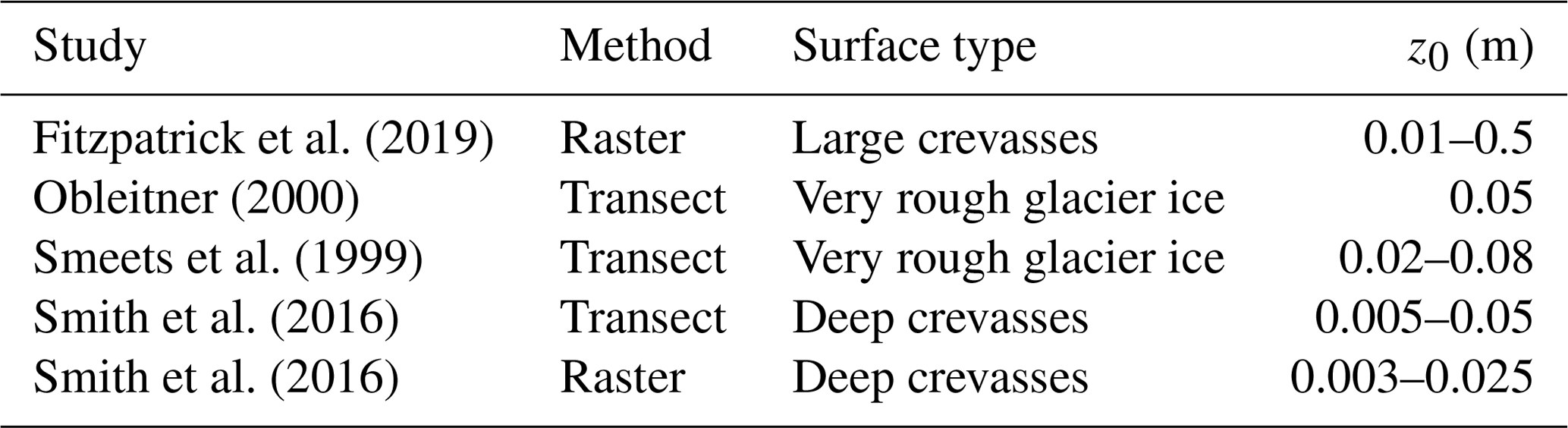
Fitzpatrick et al. (2019)Obleitner (2000)Smeets et al. (1999)Smith et al. (2016)Smith et al. (2016)

Table 1 Published aerodynamic roughness length values for crevassed glacier areas.

Recently, a series of studies (e.g. Irvine-Fynn et al., 2014; Miles et al., 2017; Smith et al., 2016) have determined z₀ values of glacier surfaces based on the bulk approach while using digital elevation models (DEMs) as the basis for calculations. Terrestrial light detection and ranging (lidar) systems (used for instance in the studies of Smith et al., 2016, Nicholson et al., 2016, and Nield et al., 2013a) constitute a powerful way to effectively produce such DEMs. However, they are very expensive (Uysal et al., 2015) and limited in the area they cover (Irvine-Fynn et al., 2014). Thus, uncrewed aerial vehicles (UAVs), often also called unmanned aerial vehicles or drones, provide a cheap alternative to overcome these limitations (Uysal et al., 2015) because they are more flexible in their use and less limited by local topography as they provide a bird's-eye perspective. In recent years, UAVs have presented new opportunities for detailed mapping of the earth surface and have become more and more popular in the field of glaciology (Bhardwaj et al., 2016) and in Svalbard (Hann et al., 2021). The main advantage of UAVs is the possibility of collecting high-temporal- and high-spatial-resolution data at low costs (Casella and Franzini, 2016) and to overcome the gap between sparse field observations and coarse-resolution space-borne remote sensing data (Bhardwaj et al., 2016).

Several studies already investigated the z₀ values of non-crevassed (Irvine-Fynn et al., 2014; Nield et al., 2013a), debris-covered (Quincey et al., 2017), sparsely crevassed (Smith et al., 2016) or rough (van Tiggelen et al., 2021) glacier ice surfaces using different approaches. However, still little is known about the effect of heavily crevassed glacier surfaces on the turbulent heat exchange between glaciers and the atmosphere. A broader-scale, heterogeneous surface topography of obstacles (i.e. crevasses) makes the definition of z₀ values challenging (Quincey et al., 2017). Typical values of z₀ on glacier ice range from less than 0.0001 m for smooth ice to 0.02–0.1 m for rough glacier ice (Brock et al., 2006; Smeets et al., 1999; van Tiggelen et al., 2021), but published z₀ values for large and deep crevasses are rare. Table 1 gives a closer overview of such published aerodynamic roughness values and shows z₀ values up to 0.5 m for large crevasses (Fitzpatrick et al., 2019). Furthermore, most surface energy balance models only consider one single z₀ value for the whole glacier (commonly 0.001 m; Smith et al., 2020), regardless of any spatial and temporal variability (Quincey et al., 2017). The aerodynamic roughness length is a key parameter for the calculation of turbulent fluxes (Chambers et al., 2020) since a change in z₀ by an order of magnitude can double the estimated turbulent fluxes (Brock et al., 2006; Munro, 1989). The uncertainty in z₀ values therefore presents a serious challenge for the calculation of surface ice melt (Smith et al., 2016), and its accurate parameterisation is crucial, especially for complex ice surfaces.

The objective of this study is to assess the application of UAVs for capturing spatially variable z₀ values of heavily crevassed ice surfaces. A photogrammetry method is used to build DEMs of the mapped glaciers from the aerial images, which are then utilised to estimate the aerodynamic roughness length of crevassed tidewater glaciers in Svalbard. The main advantage of this approach is that increasingly available UAV technology can be used to estimate turbulent fluxes that are usually difficult to measure in the field. Furthermore, the chosen DEM approach allows glaciers to be divided into areas of different aerodynamic roughness length values, leading to a better spatial representation of the turbulent fluxes and therefore surface ice melt on glaciers.

2 Data and methods

The following section describes how a DEM was generated from aerial imagery of crevassed glaciers in Svalbard. Images were obtained using off-the-shelf UAVs. In addition, different methods to calculate the aerodynamic roughness length from the DEMs are introduced.

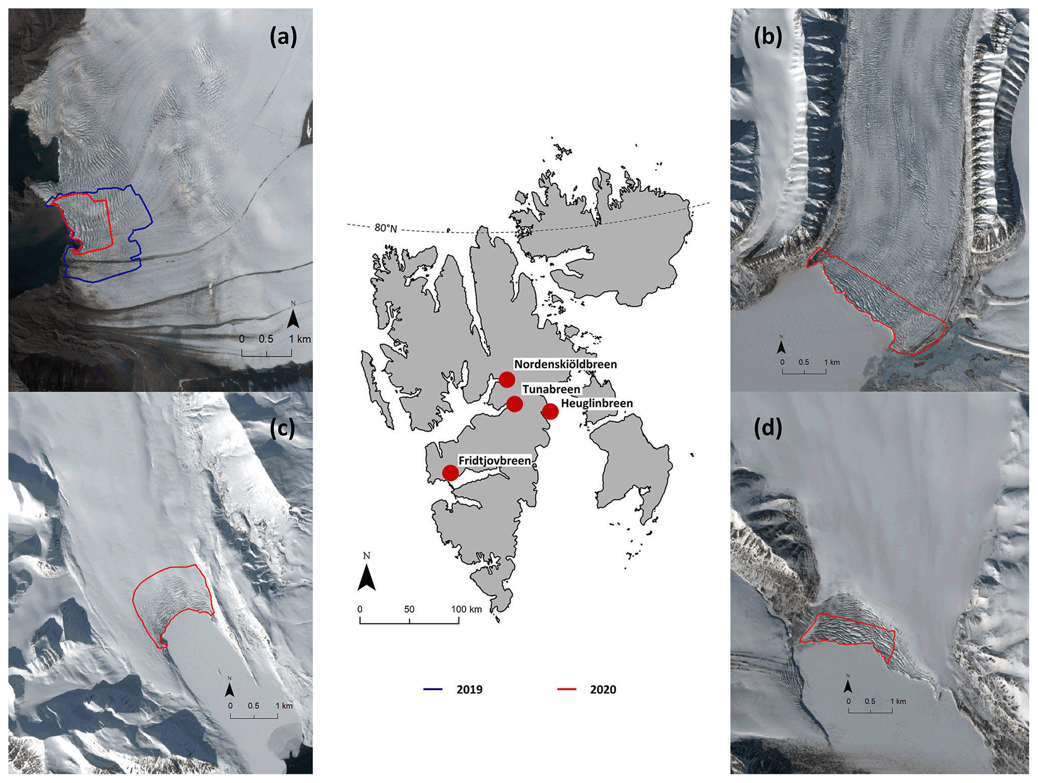
Figure 1 Field sites: map of Svalbard with marked locations of the investigated tidewater glaciers (red dots). Additionally, Sentinel-2 satellite images (ESA, 2020) of the glaciers Nordenskiöldbreen (a), Tunabreen (b), Fridtjovbreen (c) and Heuglinbreen (d) taken in the according week of fieldwork provide a closer look. The lines mark the mapped front area for each glacier in 2019 (blue) and 2020 (red).

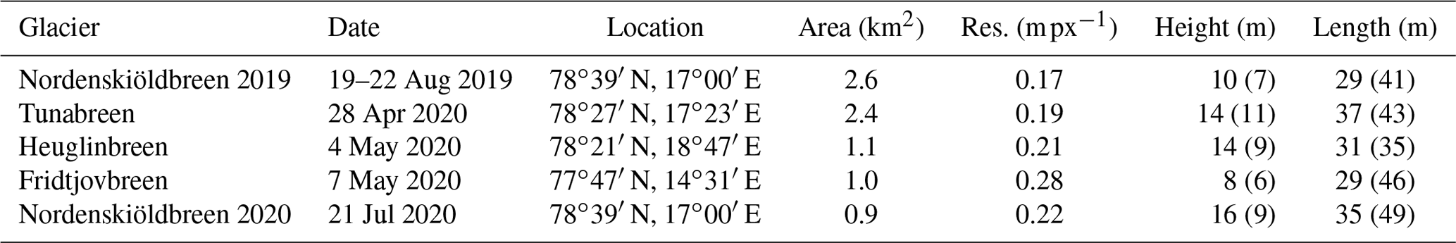
Table 2 Overview of the tidewater glaciers visited and the date of their UAV survey. Additionally, the size of the mapped area and DEM resolution, as well as the average height and length of roughness elements for a up-/down-glacier (cross-glacier) wind direction are listed.

2.1 Field sites

Four heavily crevassed tidewater glacier termini in central Spitzbergen (see Fig. 1 and Table 2) were visited during three field campaigns. Nordenskiöldbreen was visited in summer 2019 and 2020. In spring 2020 further fieldwork was conducted on Fridtjovbreen, Heuglinbreen and Tunabreen. Fridtjovbreen is a single tidewater glacier of about 13 km length, flowing southwards and terminating in Van Mijenfjorden on the western side of Spitzbergen island. Here precipitation and temperature are relatively high with an annual temperature of about −4 ^∘C and precipitation of up to 1000 mm (Hanssen-Bauer et al., 2019). Both Nordenskiöldbreen and Tunabreen are outlet glaciers (flowing from northeast to southwest) draining the large Lomonosovfonna ice cap, where the precipitation usually is lower than on the west coast (Hagen et al., 1993). While Nordenskiöldbreen is a roughly 15 km long, wide tidewater glacier terminating in Billefjorden, Tunabreen is narrower, with a length of about 20 km and terminating in Tempelfjorden. Additionally, both Tunabreen and Fridtjovbreen are known to have experienced a surge event. While the surge on Fridtjovbreen already happened during the 1990s (Murray et al., 2012), Tunabreen surged more recently in the years 2003 to 2005 and had another advance of the glacier front about 10 years later (Ericson et al., 2019). Heuglinbreen is a tidewater glacier flowing southwards and terminating into Mohnbukta, a bay on the east coast of Spitzbergen. This region is known to be particularly cold (annual temperature of about −10 ^∘C) and dry (annual precipitation up to 700 mm) (Hanssen-Bauer et al., 2019).

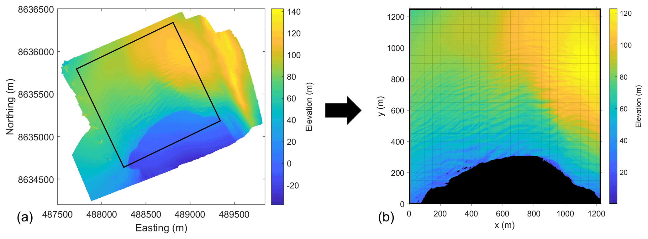
Figure 2 The originally mapped DEM (a) of Fridtjovbreen was rotated and cropped (black frame) before being used for the model calculations. Additionally, the elevation values of the sea ice area were removed, and the whole DEM was divided into sub-grids of 50 m × 50 m (b).

2.2 Field data collection

UAV-based aerial imagery was collected during each fieldwork campaign with off-the-shelf UAVs (a DJI Mavic 2 Enterprise and a DJI Phantom 4 Pro). In order to have a sufficient resolution of the crevasse fields, a target DEM resolution of about 0.25 m px⁻¹ was chosen. To achieve this DEM resolution, the UAV imagery aimed for a ground sampling distance (GSD) of at least 0.1 m px⁻¹, a forward overlap of 90 % and a side overlap of 80 %. During fieldwork the UAVs were planned to operate at an altitude of 200 $\mathrm{m}\mathrm{a}.\mathrm{g}.\mathrm{l}.$ (above ground level), taking nadir-viewing pictures. Flights were conducted with pre-programmed waypoints and a run separation of 70 m. Since information about the glacier surface elevation was unknown to the UAV, the true altitude above the glacier surface was typically less than 200 m. As a result, the GSD ranged between 0.04 and 0.07 m px⁻¹, and the subsequent DEM resolution ranged between 0.17 and 0.28 m px⁻¹ (see Table 2).

2.3 DEM generation and preparation

The high-resolution images from the UAVs were processed with a structure-from-motion (SfM) multi-view stereo (MVS) photogrammetry method using Agisoft Metashape version 1.6.2 (Agisoft LLC, 2020). Building DEMs in Agisoft is a three-step process: image alignment, construction of a dense cloud and DEM generation (Verhoeven, 2011). The software runs on a fully automatic workflow. However, the whole processing comes along with many parameter settings that can be selected to improve the DEM quality depending on the input data and the output purpose. To determine an ideal set of parameters for our approach, many different combinations of settings were tested, leading to the optimised final settings (see Dachauer, 2020). Due to the inaccessibility of the glacier surface, no ground control points (GCPs) could be placed on the mapped area for georeferencing. No alternative georeferencing platforms such as real-time kinematic correction (Chudley et al., 2019) were available. While this is a recommended procedure for future applications of this technique, we point out that computation of z₀ requires quantification of relative topographic differences, and so the impact of this shortcoming is minor.

Before starting the model calculations of the aerodynamic roughness length, the DEMs obtained from the SfM processing were rotated in such a way that the glacier flow direction corresponds to the column alignment of the DEM, with the front at the lower part (see Fig. 2). This allowed for the estimation of z₀ values for the following four wind directions: down-glacier, up-glacier and cross-glacier from both sides. Furthermore, the DEMs were cropped to a shape that contains the most crevassed zones. This area is specific to each glacier and varies significantly due to the differences in glacier size, time available for mapping, number of UAV batteries and limitations due to GPS interference. The sea ice and water area in front of the glaciers was removed since it makes no contribution to the turbulent heat exchange of the glacier.

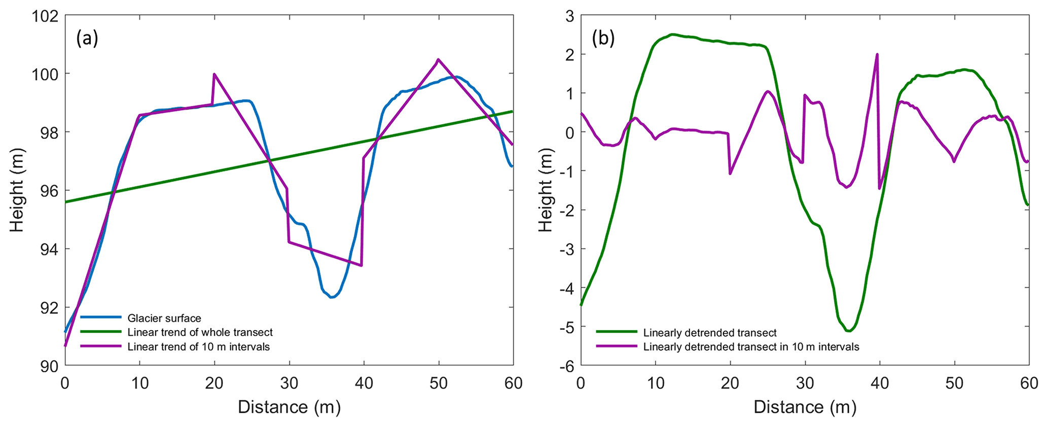
Figure 3 Graph (a) shows a random transect of two roughness elements on Fridtjovbreen (blue line). The transect is linearly detrended either over the whole profile (green) or in 10 m intervals (purple). Graph (b) illustrates the linearly detrended surface data applied at the whole transect (green line) or applied at 10 m intervals (purple line).

This study assumes that the mean airflow is blowing parallel to the slope of the glacier. This means that the glacier slope has no effect on the aerodynamic roughness (Fitzpatrick et al., 2019). Furthermore, it justifies the assumption that the aerodynamic roughness is in the first place influenced by the macro-structure of the surface (crevasses, large obstacles, etc.) and not only by small-scale surface roughness on the crevasse obstacles. In other words, only looking at the small-scale surface roughness elements would lead to a wrong roughness parameterisation since they might be located on the inner side of a large-scale roughness obstacle not exposed to the whole mean airflow. Accordingly, the chosen grid size must be large enough to include the macro-structure of the surface because small-scale roughness elements alone do not represent the real topographic expression. Linear detrending over long baselines manages to represent areas of high curvature (Smith, 2014) and is therefore appropriate for this purpose. Figure 3 presents the impact and importance of the chosen sub-grid size (i.e. length of detrended transect) on the modelled surface roughness. The blue line in Fig. 3a shows a random transect of two roughness elements of 30 m width on Fridtjovbreen. Two linear detrending methods were applied to the surface data of this illustration. First, the green line detrended the whole transect. Second, the transect was detrended in 10 m intervals (purple line). The detrended data (Fig. 3b) show that the 10 m grid size only captured the small-scale surface roughness of the obstacles (purple line). In contrast, the linearly detrended transect length of 60 m (green line) managed to represent the two large roughness elements. Therefore, a sub-grid size of at least the width of an average obstacle should be chosen to account for the macro-structure surface roughness of the crevassed glaciers. On average, the mapped tidewater glaciers had obstacle widths between 30 and 50 m (calculated according to the transect method of Munro (1989), see Table 2). Thus, the final DEMs were subdivided into rectangular sub-grids of 50 m × 50 m (grid in Fig. 2), each estimating one z₀ value.

2.4 Models for aerodynamic roughness length estimation

The aerodynamic roughness length was calculated for each DEM sub-grid and all four wind directions with five models after 2D linear detrending (see Fig. 3). The most common models in glaciology for calculating z₀ using the bulk method are based on the work of Lettau (1969), who developed the following equation for the bulk aerodynamic roughness length:

$$\begin{array}{}\text{(1)}& z_{\mathrm{0}}=c_{\mathrm{d}}{h}^{\ast }{\displaystyle \frac{s}{S}},\end{array}$$

where h^∗ is the effective obstacle height (m), s is the silhouette or frontal area of the obstacle (m²), and S is the horizontal ground area (m²). The value c_d=0.5, first proposed by Lettau (1969), corresponds to the average drag coefficient of a characteristic roughness element.

Table 3 Overview of parameters from Eq. (1) of Lettau (1969) used for the z₀ calculation of each model.

The definition of the parameters of Eq. (1) is more complex in glacial environments since the individual roughness elements are non-uniform and vary substantially in height, size and density (Chambers et al., 2020). Therefore, the original equation has been adjusted and further developed in several studies, leading to the five different models used in this study (Table 3). The five models can be subdivided into two groups according to how they determine and measure roughness elements. One group counts the number of roughness elements in a transect (hereafter called the “transect method”), while the other group is based on a raster approach (hereafter called the “raster method”) using every DEM cell value for the calculation of z₀. The choice of the models is justified by comparing results of the two methods and to give further insights into the impact of variable parameterisation on z₀ estimates for each method.

Two models using the transect method were included in this study, only differing in their definition of the effective obstacle height h^∗ (m). Each row of the sub-grid was detrended and treated as a separate transect of length X (m), whereof the transition frequency f from below to above the mean elevation was recorded (often referred to as “zero-up-crossing” in literature) for the calculation of the transect z₀ value. Thus, the final z₀ value for each sub-grid was then calculated by averaging the individual transect z₀ values within the sub-grid. First, the Lettau model calculates h^∗ by taking the average vertical extent of the detrended roughness elements, as described by Lettau (1969). Second, the Munro model simplifies Eq. (1) of Lettau (1969) such that the height of roughness element h^∗ is calculated by taking twice the standard deviation of elevations along the detrended transect, as described by Munro (1989). In contrast to the study of Munro (1989), which used wind-perpendicular surface transects for the roughness calculation, we used wind-parallel profiles for both models of the transect method. This is because if a crevasse is aligned perpendicular to the prevailing wind direction, a wind-perpendicular transect is not able to detect the crevasse, yielding a relatively low z₀ value (for further explanation, see Smith et al., 2016). Thus, such an adaptation is essential for heterogeneous, anisotropic and naturally streamlined roughness elements as those investigated in this study since wind systems are influenced by the large-scale catchment topography and therefore often flow up or down the glacier (Quincey et al., 2017). The transect method presents a simple approximation of the roughness elements across a profile and, in contrast to the raster method, assumes all roughness elements to be of equal height, uniformly distributed, isotropic and not affected by any sheltering effects.

The raster method is also based on Eq. (1) of Lettau (1969), but the elevation differences between two adjacent cells define the surface roughness in the end. In the raster method all sub-grids were detrended row-wise, and areas below the detrended plane were neglected, assuming that they would be effectively sheltered. Three models following the raster method were included in this study. First, the Smith model was based on the “DEM-based” approach described by Smith et al. (2016). The effective obstacle height h^∗ was calculated as the mean elevation of all the cells of each row above the zero plane. The second model of the raster method (hereafter called Chambers model) was based on the “DEM method” described by Chambers et al. (2020). Its only difference to the Smith model is again the definition of the effective obstacle height h^∗, which is twice the standard deviation of elevations above the detrended plane. The third model of the raster method (hereafter called Fitzpatrick model) was based on the “block estimation” described by Fitzpatrick et al. (2019). While the two previous raster methods calculated some of the parameters row-wise, this method followed a moving window approach (see Table 3). The obstacle height h^∗ corresponded to the mean of all the detrended elevation values above the zero plane within the window. In this study, a window size of 30 m was chosen, which corresponded to the lower estimation of an average roughness element on the investigated glaciers (see Table 2). For all three models, s and h^∗ were calculated individually for each row of the sub-grid (moving window for the Fitzpatrick model). Accordingly, the ground area S was assigned to the area of the sub-grid (moving window), and the final z₀ value for each sub-grid was then calculated by taking the mean of its row (moving window) values.

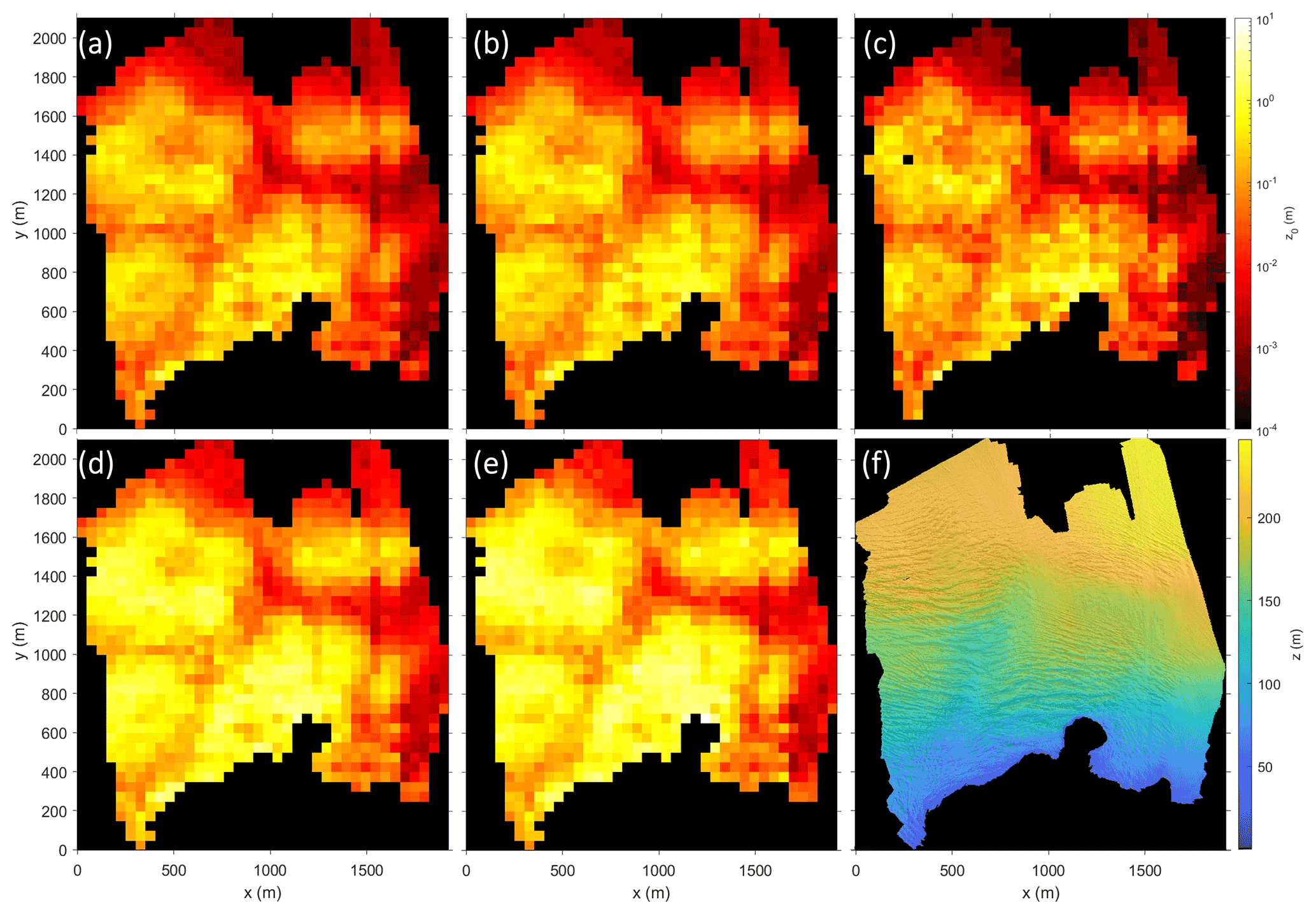
Figure 4 Variability in z₀ values for Nordenskiöldbreen (2019) depending on the calculation models – Smith (a), Chambers (b), Fitzpatrick (c), Munro (d) and Lettau (e) – for a sub-grid size of 50 m × 50 m and a down-glacier wind direction. Graph (f) shows the DEM with the underlaid hillshade layer.

3 Results

The DEMs obtained from the UAV-based imagery and processed with the SfM-MVS method illustrate that the crevasses of the mapped glaciers are in general aligned perpendicular to the glacier flow direction. The crevasses closer to the front are often deeper and larger in terms of spacing (width of crevasse opening) compared to crevasses located upstream of the glacier (see Fig. 4). The DEMs were then used to calculate the aerodynamic roughness lengths with the two transect method models and the three raster method models. The results (e.g. Figs. 4, 6 and 7) show that the spatial variability in z₀ values across the mapped area is up to 3 orders of magnitude. In general, the larger a roughness element is, the larger its aerodynamic roughness length will be. The largest z₀ values (decimetre to metre scale) were found close to the glacier front, where crevasses are big and steep, using the transect methods and for winds blowing parallel to the flow direction of the glacier. The lowest values (millimetre to centimetre scale) are estimated with the raster methods for smooth, crevasse-free ice and for cross-glacier wind directions.

3.1 Model results

Figure 4 shows the estimated aerodynamic roughness length values for each of the five applied models for the down-glacier wind direction on Nordenskiöldbreen (2019). The results reveal that all models agree on the relative spatial z₀ patterns across the glacier. Accordingly, for the flatter and less crevassed part (e.g. to the right of the mapped area on Nordenskiöldbreen), all models show lower sub-grid z₀ values (red) compared to the heavily crevassed part close to the glacier front (yellow). To further investigate the relative agreement between the models a statistical correlation test on the z₀ data of Nordenskiöldbreen (averaged over all four wind directions) was conducted. The correlation test showed that all models are strongly correlated to each other, leading to R² values of 0.877 and higher (Dachauer, 2020). A similar correlation was also observed for the other glaciers. While this indicates that the z₀ values are correlated, it does not provide any conclusion about the quality of the individual models.

Table 4 Overview of mean z₀ values (m) for each glacier and model either for the down-glacier or cross-glacier (left-to-right) wind direction.

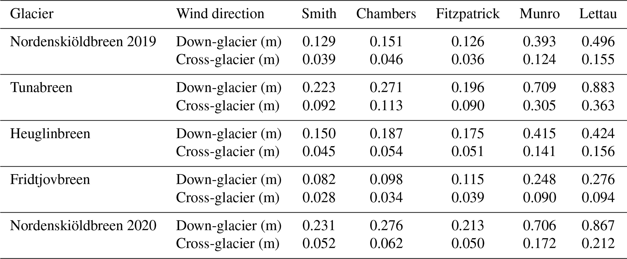
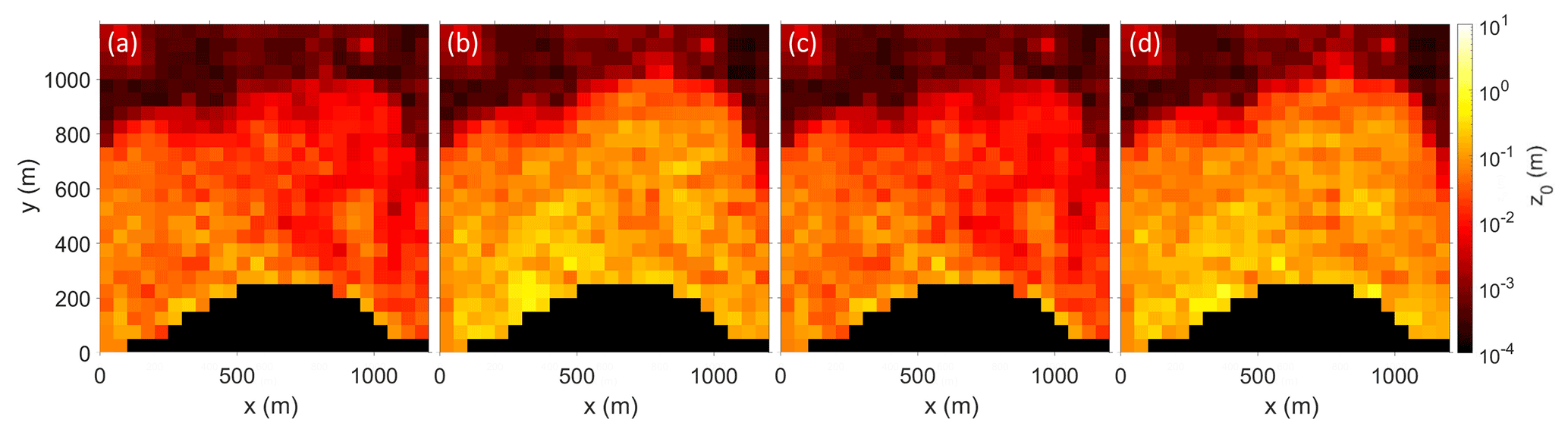
Figure 5 Variability in z₀ values for Fridtjovbreen depending on the wind direction for a sub-grid size of 50 m calculated with the Smith model. Winds blowing across the glacier either from the left-to-right (a) or right-to-left (c) produce smaller z₀ values than down-glacier (b) or up-glacier (d) wind systems.

Figure 4 further illustrates that the absolute values of the Munro and Lettau models show greater roughness values on the same sub-grid than the other three models. In more detail, the Lettau model estimates are generally greater than those of the Munro model and Chamber z₀ values greater than those of the Smith model (see also Table 4). The three models of the raster method provide sub-grid z₀ values of about 0.001 m for slightly crevassed areas and up to 1 m for heavily crevassed areas. The same sub-grids calculated with the two transect methods produced z₀ values which are locally up to 1 order of magnitude larger. Table 4 illustrates the down-glacier and cross-glacier (left-to-right) mean z₀ values for all glaciers and models. Table 4 also shows that average z₀ values across the glacier vary almost up to half an order of magnitude between the models. In summary, despite the clear relative agreement between the models, the estimated magnitude of the z₀ values varies substantially between the models – especially between the raster and transect method models. This might be explained by the fact that the transect method does not account for sheltering of an obstacle (Smith et al., 2016). The raster method on the other hand assumes the areas below the detrended plane to be effectively sheltered. This plane indicates how far the effective turbulent mixing advances into the crevasses, and the corresponding z₀ values are expected to be lower if the sheltering effect is considered (Nicholson et al., 2016).

3.2 Wind direction variability

Figure 5 illustrates the map of Fridtjovbreen with z₀ values obtained with the Smith method for all four wind directions. The results show that z₀ values are higher for wind directions that face the crevasses perpendicularly (i.e. up- and down-glacier) and lower for wind that blows parallel to the elongated crevasse features (i.e. cross-glacier). The two cross-glacier (up- and down-glacier) wind directions lead to very similar z₀ values since they are both calculated on the same transect but from opposite wind directions. Since crevasses are mainly oriented perpendicular to the glacier flow direction, the mapped areas show a strongly anisotropic pattern of the glacier surface. This wind dependency effect is visible on all five applied models and is independent of the roughness element size. However, Fig. 5 illustrates that larger roughness elements, which can be found close to the glacier front for instance, present a stronger wind dependency because they vary more strongly with changing wind directions (from decimetre to metre scale) compared to areas that are less crevassed like on the upper part of Fridtjovbreen (similar z₀ values in millimetre scale for all wind directions).

Figure 6 Boxplot visualisation of sub-grid z₀ values for all four wind directions and each applied model determined on Fridtjovbreen. The wind direction is either down-glacier (orange), up-glacier (green), cross-glacier from right to left (blue; rtl) or cross-glacier from left to right (red; ltr). Whiskers are visualising the variability outside the upper and lower quartiles up to 1.5 times the interquartile range.

Figure 7 Variability in z₀ values for the glaciers Tunabreen (a) and Heuglinbreen (b) calculated with the Smith model for a down-glacier wind direction and a sub-grid size of 50 m.

Additionally, Fig. 6 shows the boxplot graph of z₀ estimates illustrating the wind direction dependency of z₀ values on Fridtjovbreen. The boxplot z₀ medians of all models vary in a range of 0.012 to 0.037 m for crosswind directions and 0.058 to 0.2 m for up- and down-glacier wind systems. The mean and median values between up- and down-glacier wind systems (left-to-right and right-to-left crosswinds, respectively) never differ by more than 10 % and only rarely more than 5 % independently of the chosen model or glacier. In summary, the wind direction has a large impact on the resulting aerodynamic roughness length values. Its effect on average or median z₀ values slightly exceeds the model variability. Locally, however, both mean and median z₀ estimates can vary by about 1 order of magnitude with changing wind direction.

3.3 Glacier variability

All glaciers showed a similar range of z₀ values on the decimetre to metre scale for heavily crevassed areas and millimetre to centimetre scale for less crevassed areas (see Figs. 4, 5 and 7). However, the results of Table 4 show that the mean z₀ values for the Smith model and down-glacier wind direction are somewhat larger on Tunabreen (0.223 m) and the extract of Nordenskiöldbreen mapped in 2020 (0.231 m) compared to the other glaciers. The same mean z₀ values on Nordenskiöldbreen measured in 2019 are lower, at only 0.129 m. Heuglinbreen (0.15 m) and especially Fridtjovbreen (0.082 m) show lower mean z₀ values than the glaciers mentioned above. Nevertheless, all the patterns found in this study (e.g. between wind direction or sub-grid size and the z₀ values) are independent of the glacier and vary (if even) only in magnitude rather than relative patterns in between the glaciers.

On a side note, it is interesting to study the results of Nordenskiöldbreen 2019 and 2020 in more detail. The comparison provides insights into the inter-annual temporal variability in z₀ values for 2 consecutive years. The mapped area in summer 2020 (1 d of fieldwork) was smaller compared to the field campaign approximately 1 year earlier in 2019 (3 d of fieldwork). Therefore, only the overlapping area has been used for the temporal variability investigation. Furthermore, for this particular comparison the DEM extract of Nordenskiöldbreen 2019 (0.17 m px⁻¹) was resampled to the resolution of the Nordenskiöldbreen 2020 DEM (0.22 m px⁻¹). The z₀ values on Nordenskiöldbreen were very similar for the 2 consecutive years. The mean z₀ value for the Smith model and down-glacier wind direction in 2019 was, at 0.25 m, only slightly greater than the corresponding value of 0.23 m at the same area 1 year later. The observations are in line with other studies (i.e. Fitzpatrick et al., 2019), which also did not observe a large difference in z₀ estimates for the same location over 2 consecutive years. Relatively, the mean z₀ values never deviated more than 20 % and mostly less than 10 % between the 2 years. In summary, the differences in z₀ estimates across the models exceed the inter-annual temporal z₀ variability by far, independently of the model calculation.

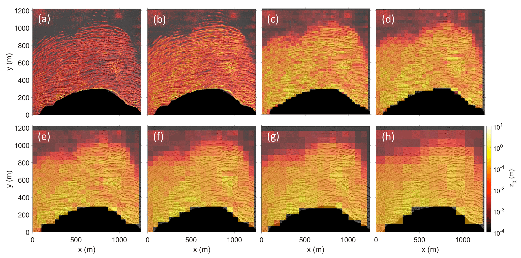
Figure 8 Scale-dependent z₀ values for the Smith model and down-glacier wind direction applied on Fridtjovbreen for sub-grid size resolutions of 5 m (a), 10 m (b), 30 m (c), 40 m (d), 50 m (e), 60 m (f), 70 m (g) and 100 m (h) with underlaid hillshade layer for orientation.

3.4 Sub-grid size dependency

The mapped glacier areas were divided into sub-grids with a grid size of 50 m × 50 m to account for the spatial variability in z₀ on the glacier. However, to investigate the grid size dependency of the sub-grids on z₀ values, a small case study on the glacier Fridtjovbreen was conducted. The Smith model with a down-glacier wind direction was used to calculate aerodynamic roughness lengths for sub-grid sizes between 5 and 150 m. Figure 8 illustrates the scale dependency of z₀ values to the selected sub-grid size. The results show that a grid size of 5 to 10 m mostly produces z₀ values on a scale of centimetres. Between sub-grid sizes of 10 and 50 m a higher grid size results in higher z₀ values. From 50 m onwards, the z₀ values are mostly at the decimetre scale and do not change substantially. This behaviour was also observed with the other models and for all wind directions. For small sub-grid sizes, the z₀ values are likely representing microtopography rather than the macro-scale surface roughness of the crevasses.

Figure 9 Scale dependency of mean z₀ values for the five applied models and a down-glacier wind direction on Fridtjovbreen with chosen sub-grid sizes from 5 to 150 m. The black line indicates the chosen grid size of 50 m which incorporates the upper boundary of the average obstacle sizes between 30 and 50 m found on all glaciers (see Table 2).

Figure 9 summarises the mean z₀ results of the mentioned case study for the down-glacier wind direction. For all the models, the mean z₀ values increased by at least half an order of magnitude between a sub-grid size of 5 and 150 m. All models showed a similar pattern with strongly increasing z₀ values for small grid sizes (5 to 30 m) and only slightly increasing estimates afterwards. Grid sizes of 70 m or more lost their strong scale dependency effect, leading to stable z₀ estimates. The same effect is visible in Fig. 8, where the chosen grid size of 50 m represents similar z₀ values (colours) as the higher grid sizes for the same location while still providing a considerable grid resolution.

4 Discussion

4.1 Model inputs for aerodynamic roughness length estimation

4.1.1 Validation of digital elevation model accuracy

The obtained DEM resolution with the SfM-MVS method (about 0.25 m) was accurate enough to capture the large crevasse structures. Given the advantages of a UAV compared to other devices (e.g. low cost, applicable to inaccessible areas; Hann et al., 2021), this study shows that UAVs provide a reliable and effective way of data gathering for aerodynamic roughness length estimation on glaciers. Nevertheless, the depth of the crevasses must be seen as a minimum depth, and the crevasses might penetrate further into the glacier than actually measured. This is due to snow bridges or the lack of reflected light from the deep crevasses. The latter prevents the SfM-MVS methods from correctly constructing the deeper parts of the crevasse. Additionally, the lowest points of the crevasses are very narrow and may not be captured accurately (Ryan et al., 2015). However, in an aerodynamic context those narrow crevasses are not likely to have a significant influence on the heat exchange since they lie below the penetration depth of effective turbulent mixing (Nicholson et al., 2016). Equation (1) of Lettau (1969) and the transect methods do not define any penetration depth limit. The raster method, however, assumes that effective roughness only depends on the roughness elements above the detrended plane level, which indicates how far the effective turbulent mixing advances into the crevasses.

In the scope of this study the absence of GCPs was also considered. GCPs can significantly increase the georeferencing accuracy of the DEMs (Chudley et al., 2019). However, it was practically impossible to place GCPs on the crevassed glacier surfaces due to safety reasons. Therefore, the georeferencing information was provided only from the on-board GPS and the measurements of camera orientation (James et al., 2017). In other words, the positional accuracy of the DEM is limited by the internal GPS system of the UAV, which has a relatively low accuracy (Federman et al., 2017). However, the objective of this study was not to obtain a high-accuracy DEM but rather a precise DEM combined with a detrending approach for the investigation of the effect of relative distances. Therefore, the given hover accuracy of ± 1.5 m horizontally and ± 0.5 m vertically for both UAVs (DJI, 2017, 2019) was considered sufficient (Dachauer, 2020).

Nevertheless, a comparison with Sentinel-2 satellite data (ESA, 2020) revealed horizontal positioning errors (data not shown). The deviation was classified as a systematic offset (for more details see Dachauer, 2020). The detected small horizontal distortions of about 1.7 % (horizontal length deviation in percent of DEM compared to the Sentinel-2 satellite image) mainly occurred on the ends of the DEMs. This is a typical feature appearing when only using nadir imagery and is related to self-calibration because the reconstruction software is not able to derive the accurate radial lens distortion leading to a systematic “doming” DEM deformation (James and Robson, 2014). However, a systematic error is of low significance for this study since only the relative accuracy of the roughness elements (i.e. distortion) influences the estimation of the aerodynamic roughness lengths. Furthermore, the influence of a small distortion of a few percent or several metres across the mapped area on the resulting z₀ values is minor compared to other parameters such as wind direction, model calculation or scale dependency. For example, a distortion of 2 % led to a change in z₀ of about 4 % (Dachauer, 2020). This means that the obtained DEMs in this study are a reliable data source to estimate the aerodynamic roughness length.

4.1.2 Scale dependency

Many studies have investigated and encountered the dependency of z₀ estimates on the size of the sub-grid or the transect length (e.g. Fitzpatrick et al., 2019; Miles et al., 2017; Rees and Arnold, 2006) and reported that larger sub-grids or longer transects cause z₀ values to increase (Chambers et al., 2020). Also the case study conducted on Fridtjovbreen data revealed that the z₀ values increase with larger grid size independently of the chosen glacier, model or wind direction. This can be explained by the fact that glaciers often have heterogeneous roughness elements (Quincey et al., 2017). In general, it needs to be considered that the selection of an appropriate grid size comes with a large potential uncertainty. To find the most meaningful grid size a comparison with independent methods like aerodynamic wind profiles is recommended (Chambers et al., 2020). Since this option was not available in our study, the validity of the chosen grid size has been evaluated theoretically. The grid size in our models corresponds to the ground area S, whose definition requires the grid size to be the size of one individual roughness element (Lettau, 1969), which is 30 to 50 m (see Table 2). According to Smith (2014), the definition of “roughness” is related to the grid scale that separates the grain roughness (representing the texture of a roughness element) and the form roughness (corresponding to the form drag of the roughness element itself). The grid size at which the transition from grain to form roughness occurs provides a useful reference point and can be found as a kink in the trend line of a figure plotting z₀ values against grid sizes (Shepard et al., 2001; Smith, 2014). Accordingly, given the large roughness elements investigated in our study, the “grain” roughness was assumed to belong to the texture on the crevasses. Thus, the transition from grain to form roughness is again located somewhere between a sub-grid size of 30 to 50 m (see Fig. 9). Therefore, in this study the grid size of 50 m was chosen since it is the smallest resolution possible to still include the size of an average obstacle. Typical z₀ estimates for smooth glacier ice, which for instance can be found on the upper part of Fridtjovbreen, have a length of about 1 mm (Brock et al., 2006). The choice of a 50 m grid size can further be justified since Fig. 8 shows that grid sizes below 30 m do not provide high enough values and therefore do not agree with literature values.

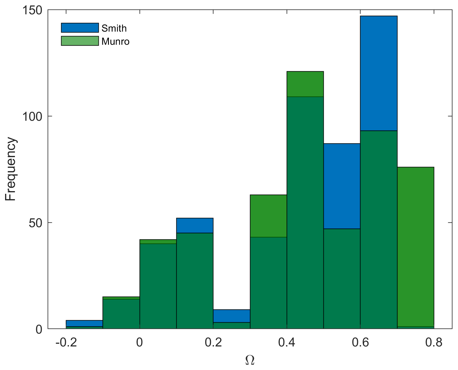
Figure 10 Anisotropy ratio values for the two models of Smith (blue) and Munro (green) calculated for sub-grid z₀ values on Fridtjovbreen. The dark green colour corresponds to an overlapping of both models. A positive ratio towards 1 means that parallel winds (up- and down-glacier) are dominant over perpendicular winds (cross-glacier).

4.2 Estimated aerodynamic roughness length

4.2.1 Wind direction dependency

The wind direction has a large impact on the magnitude of the z₀ values on glaciers since they contain many anisotropic roughness elements (Chambers et al., 2020). Our results confirmed this statement and further revealed that larger roughness elements in general present a stronger wind dependency (see Fig. 5). The wind dependency effect was additionally investigated with the calculation of the anisotropy ratio Ω (see Smith et al., 2006, for further explanation):

$$\begin{array}{}\text{(2)}& \mathrm{\Omega }={\displaystyle \frac{z_{\mathrm{0}\parallel }-z_{\mathrm{0}⟂}}{z_{\mathrm{0}\parallel }+z_{\mathrm{0}⟂}}},\end{array}$$

where subscripts ∥ and ⟂ denote parallel and perpendicular to the ice flow direction, respectively. Figure 10 illustrates a histogram of the sub-grid's Ω values on Fridtjovbreen for the Smith (blue) and Munro (green) model. The results show that the sub-grid z₀ values are strongly anisotropic all across the glacier, whereas wind directions parallel to the flow direction are dominant (since values are mostly positive). Both the raster (here Smith model) and the transect methods (Munro) show a similar pattern with the highest frequency at the range of 0.4 to 0.7 (Smith) and 0.4 to 0.8 (Munro). Although Tunabreen has still mostly positive ratio values, it is the glacier with the least anisotropic behaviour of all investigated glaciers. The importance of wind direction can be observed in many studies (e.g. Fitzpatrick et al., 2019; Munro, 1989; Smith et al., 2016) and is found to be the strongest on ablation zones where elongated features like meltwater channels and crevasses are frequent. Thus, wind directions that face these features perpendicularly lead to higher z₀ values due to an increased form drag (Fitzpatrick et al., 2019). Winds are in general very likely to blow in the direction of the mean slope angle or in a down-slope wind direction (e.g. Fitzpatrick et al., 2019; Karner et al., 2013). This is due to katabatically forced down-slope winds, which are common over the glacier terminus (Munro, 1989). Nevertheless, Esau and Repina (2012) found the katabatically forced wind systems to be of less significance for polar tidewater glaciers. This highlights the influence and importance of wind direction on effective z₀ values. Furthermore, the wind direction dependency reveals the temporal variability in the aerodynamic roughness length due to changing wind directions from daily up to seasonal timescales.

4.2.2 Variability across the glaciers

Since almost no values of z₀ for heavily crevassed glaciers are available in the literature, the validation of the results of this study is difficult. The roughness elements investigated by previous studies (see Table 1) were smaller than the crevasses of this study. Therefore, it is expected that the z₀ values obtained here should be larger. This was the case, although there was a significant spread of z₀ values across the estimation models. The mean results in Table 4, and there in particular the raster method results, fall mostly within the same order of magnitude. The range suggested by Fitzpatrick et al. (2019) fits most of the results from this study across different methods and glaciers. Outside the field of glaciology, the heavily crevassed glaciers might most effectively be compared with villages since buildings can have similar obstacle density and height. Accordingly, the z₀ values for villages are about 0.2–0.4 m (Abbas et al., 2021), which lie within the range of estimated roughness values in this study.

In general, Tunabreen and Nordenskiöldbreen (especially the part mapped in 2020) show higher z₀ values than Fridtjovbreen and Heuglinbreen. This is in good agreement with the average length and height of roughness elements estimated for each glacier in Table 2. The crevasses on Tunabreen and Nordenskiöldbreen are generally deeper and steeper than the crevasses on the other two glaciers. This might be explained by different dynamical behaviour, leading to higher z₀ values. In general, a faster flowing glacier leads to more crevasses in the terminus area of the glacier and a larger area of crevassing (Błaszczyk et al., 2009). Additionally, Tunabreen was recently surging, which usually leads to very chaotically aligned crevasses (Mansell et al., 2012). Thus, these results are in line with the observation that the anisotropy ratio value Ω is lowest on Tunabreen as perfectly aligned roughness elements increase the anisotropy effect. However, comparing average z₀ values among different glaciers is challenging because the mean z₀ values depend substantially on the mapped input area and therefore the size of included roughness elements.

4.3 Model performance assessment

If the roughness elements on a plot are too densely packed, then the objects begin to interfere aerodynamically with each other (Rounce et al., 2015). They form a plateau-like new surface at their tops (Lettau, 1969) leading to a skimming flow. If this roughness density (frontal area divided by ground area) increases as far as is necessary to induce skimming flow, then the z₀ values decrease (Grimmond and Oke, 1999). Accordingly, the results from the transect methods which are not considering any sheltering effects are likely to overestimate the roughness, especially for densely packed obstacles (Nicholson et al., 2016). Several studies (e.g. Nicholson et al., 2016; Rounce et al., 2015; Smith et al., 2016) used a roughness density threshold of 20 % to 30 % (as stated by Macdonald et al., 1998) for Eq. (1) of Lettau (1969) to still be valid. In our study, all glaciers were tested with the Smith model for their roughness density. Apart from some single heavily crevassed sub-grids close to the glacier front which exceed the threshold of 30 %, all glaciers are below the given threshold with mean roughness density values between 0.1 and 0.15 for each glacier, indicating no skimming flow over the obstacles was likely. Therefore, this study assumes that Eq. (1) of Lettau (1969) also holds for heavily crevassed tidewater glaciers with respect to the sheltering effect.

The Lettau formula is based on empirical experiments of systematically placed bushel baskets for roughness simulation. Transferring the simple relation onto heterogeneous and complex surfaces as found on the heavily crevassed tidewater glaciers might lead to some uncertainties. This is because the Lettau relation for the calculation of z₀ strongly simplifies the complex surface roughness and its obstacle size, shape and density. A simplified representation of the surface roughness might fail to capture the complete range of aerodynamic processes. The Smith and Chambers models, as well as Munro and Lettau models, only differ in the definition of h^∗. An appropriate definition of h^∗ is crucial since the obstacle height is the most important control parameter over the output of z₀ (Nield et al., 2013b). Thus, the lack of a clear obstacle definition presents the main problem of the bulk method (Rounce et al., 2015), especially in crevassed glacier areas, where an apparent base level is missing (Nicholson et al., 2016). To find out which model and which definition of h^∗ might perform best, a comparison with alternative measurement methods (e.g. wind profiles) would be necessary, as is done in several studies (Fitzpatrick et al., 2019; Quincey et al., 2017; Smeets et al., 1999). For this study, however, the area of interest was inaccessible and so this validation option was impossible. In any case, it clearly can be seen that the definition of h^∗ has a lower impact on the results than the choice of the basic method (i.e. raster/transect), which particularly affects the values of the silhouette area s. The definition of the ground area S which corresponds to the chosen grid size and the according profile length is a simple approximation of the real fetch footprint. However, the simplification allows for the estimation of z₀ values for the four wind directions and additionally provides uniform parameterisation throughout all glaciers and models. The widely adopted drag coefficient of Lettau (1969) of c_d=0.5 corresponds to an average form drag effect on roughness elements. Its rationale is widely discussed since it does not necessarily hold for complex and heterogeneous locations where drag may be large due to the irregular density and shape of roughness elements. This might lead to a higher effective drag and therefore underestimated z₀ values (Quincey et al., 2017).

Turbulent fluxes already contribute a large fraction of surface ice melt (Fausto et al., 2016) and are supposed to have an even greater contribution to surface energy balance models under global warming (Smith et al., 2020). Thus, a high accuracy of estimated z₀ values is desirable. The validation of the model estimates remains a big challenge due to the lack of reference values, and it should be questioned whether the modelled z₀ values are accurate enough for energy balance models. In general, an increase in z₀ by 1 order of magnitude will more than double the value of turbulent fluxes (Brock et al., 2000). Therefore, whilst grid-size and model choice can contribute up to 1 order of magnitude uncertainty in z₀ values, it is far outweighed by the 3 orders of magnitude range in z₀ observed in the present study. Spatial variability in z₀ values caused by intense crevassing near the margin of tidewater glaciers therefore greatly exceeds the uncertainty introduced by modelling choices and can be constrained with sufficient accuracy through the methods pioneered here. Furthermore, this large spatial variability, which is commonly not considered in models, affects the partition of mass loss between frontal and surface ablation. Additionally, the relevance of further narrowing down the modelled range in the future depends a lot on the field of application. For large-scale, satellite-based investigations an average value between all models (e.g. 0.1 m) for heavily crevassed glacier areas might be a sufficiently accurate approximation. Small-scale investigations on individual glaciers on the other hand likely benefit from more accurate z₀ estimates. It is here in particular, where our study shows that UAVs are the ideal platform for investigating aerodynamic roughness length.

5 Conclusions

The heavily crevassed terminus areas of the tidewater glaciers Fridtjovbreen, Heuglinbreen, Nordenskiöldbreen and Tunabreen were mapped with UAVs to build DEMs that revealed crevasse shape information. To take into account the spatial variability across the glacier, the DEM was divided into sub-grids of 50 m × 50 m, which was assumed to be large enough to include an average roughness element while still being small enough to account for the roughness variability across the glacier. Five different models (belonging to either the transect or the raster method) were applied to each DEM sub-grid to calculate the aerodynamic roughness length. The z₀ estimates from the transect method were in general greater (up to 1 order of magnitude) than the raster method estimations. Wind direction and sub-grid size had a large impact on the z₀ estimates, again producing a range of up to 1 order of magnitude for each parameter. Winds blowing parallel to the ice flow direction produced larger z₀ values than cross-glacier winds. The chosen sub-grid size presents a large uncertainty in aerodynamic roughness length estimation. The resulting z₀ values are strongly scale dependent such that a larger grid size leads to greater z₀ values. If all parameters (i.e. model, wind direction, grid size) are included, the spread of the resulting z₀ estimates is large, ranging from below 1 mm (snow-covered, smooth glacier surface) up to several decimetres (heavily crevassed ice) or locally even more. Averaged z₀ values for down-glacier wind directions varied from 0.08 to 0.88 m depending on glacier and model. Nevertheless, all models managed to detect the same spatial variability across the glacier. The UAV approach allows several z₀ values for each mapped glacier area to be derived, which is crucial for heavily crevassed glaciers since one value would be a poor representation of the real roughness across such a complex topography. Therefore, models can now incorporate distributed z₀ estimates easily following UAV deployment, potentially leading to a better representation of turbulent heat fluxes and prediction of surface ice melt rates.

Spatial and temporal variability in crevassing and a dependence on wind direction were found to extend the range of z₀ values on tidewater glaciers. Variability caused by sub-grid size and model calculation assumptions reveal uncertainties which should be addressed by future investigations. Some degree of uncertainty also comes with the unsatisfactory georeferencing of the DEM in crevassed areas because the inaccessible topography imposes practical limitations, especially on the use of GCPs. Furthermore, future work should seek a scale-independent method for z₀ calculation and also assess model performance using meteorological measurements (e.g. wind profiles) or computational fluid dynamics simulations. In a next step, a combination of high-resolution DEMs from UAVs for reference z₀ values and satellite-based crevasse density estimates might prove valuable for future research.