the Creative Commons Attribution 4.0 License.
the Creative Commons Attribution 4.0 License.
 | 25 Nov 2021
Snow water equivalent measurement in the Arctic based on cosmic ray neutron attenuation
Anton Jitnikovitch
Philip Marsh
Branden Walker
Darin Desilets
Grounded in situ, or invasive, cosmic ray neutron sensors (CRNSs) may allow for continuous, unattended measurements of snow water equivalent (SWE) over complete winter seasons and allow for measurements that are representative of spatially variable Arctic snow covers, but few studies have tested these types of sensors or considered their applicability at remote sites in the Arctic. During the winters of 2016/2017 and 2017/2018 we tested a grounded in situ CRNS system at two locations in Canada: a cold, low- to high-SWE environment in the Canadian Arctic and at a warm, low-SWE landscape in southern Ontario that allowed easier access for validation purposes. Five CRNS units were applied in a transect to obtain continuous data for a single significant snow feature; CRNS-moderated neutron counts were compared to manual snow survey SWE values obtained during both winter seasons. The data indicate that grounded in situ CRNS instruments appear able to continuously measure SWE with sufficient accuracy utilizing both a linear regression and nonlinear formulation. These sensors can provide important SWE data for testing snow and hydrological models, water resource management applications, and the validation of remote sensing applications.
- Article
(4479 KB) - Full-text XML
- BibTeX
- EndNote


The Arctic tundra snow cover is typified by low snow depth and low snow water equivalent (SWE) when averaged over areas of a few square kilometers but extreme spatial variability in depth and SWE over distances of less than 10 m (Sturm et al., 2010, 2001; Rees et al., 2014). These features are due to a combination of low winter snowfall, wind that redistributes snow across the landscape, and high rates of sublimation during these blowing snow events. For example, total SWE is often less than 300 mm over the long winter, with up to 40 % of this snowfall sublimating during blowing snow events. Blowing snow also results in wind-scoured uplands characterized by shallow, low-density snow cover (<0.7 m; <300 kg m−3) and deep, high-density snow drifts (up to 10 m; up to 600 kg m−3) located on steep hillslopes (Marsh and Pomeroy, 1996). Within the tundra–taiga ecotone, deep drifts also occur in small shrub or tree patches. Although deep drifts are small in area, they often contain a large portion of the total landscape SWE (Gray et al., 1974; Marsh and Woo, 1981; Gray et al., 1989; Marsh and Pomeroy, 1996; Sturm et al., 2001). This spatially variable snow cover exerts important controls on many aspects of the tundra environment, including soil and permafrost temperature, permafrost processes such as ice wedge cracking, streamflow hydrology, lake level, and wildlife habitat for example. However, monitoring this snow cover remains extremely challenging (Kinar and Pomeroy, 2015).
The Arctic snow observing system has very few ground-based monitoring stations, and these are often located in areas not representative of the broader Arctic. For example, the majority of Arctic stations are typically chosen to be located at town sites, for search and rescue bases/stations, to improve military capabilities, to function as entities that legitimize national or sovereign claims, and to engage in multilateral actions to protect Arctic infrastructures (Goodsite et al., 2016). Since the 1970s many purely research-purpose Arctic environmental monitoring stations have been permanently closed (Schiermeier, 2006; Rees et al., 2014). As such, standard measurements used at these stations are either prone to considerable errors, not representative of the surrounding area, or not measured at all. For example, snowfall measurements are prone to large errors due to undercatch during high winds (Pan et al., 2016), while sublimation is seldom measured. Measurements of snow depth are typically not representative of the surrounding natural terrain as they are limited to point observations using ruler measurements or acoustic distance systems (Kinar and Pomeroy, 2015). Recent advances in methodology allow for the measurement of SWE using gamma attenuation (Kirkham et al., 2019) or global positioning systems (Koch et al., 2019) but again are limited to point or campaign-based measurements. To overcome these deficiencies, practitioners and researchers still use traditional, manual snow surveys in order to document average snow depth, density, and SWE across Arctic landscapes. Snow survey methods have well-known limited accuracy in tundra areas (Goodison et al., 1981; Pomeroy and Gray, 1995; Steufer et al., 2013; Kinar and Pomeroy, 2015) and do not allow for mapping snow cover as is needed for many Arctic research studies.
Satellite and aircraft remote sensing provide methods to partially overcome some of the limitations outlined above through the mapping of both snow cover extent and SWE. Although current satellite methods are well suited to assessing climate change impacts on snow across the entire Arctic (Derksen and Brown, 2012; Rees et al., 2014; Hori et al., 2017; Tollefson, 2017; Bush and Lemmen, 2019) and for large-scale water resource needs, they are not suited for providing snow data at the high spatial resolution required for many research needs. Airborne remote sensing methods are able to provide high-resolution snow data, but they also have certain limitations. For example, methods to map snow depth at high resolutions are available (Deems et al., 2013; Walker et al., 2020), but mapping of snow density or SWE is not (Koch et al., 2019). SWE along-flight transects are available using airborne gamma methods but have limited applicability in the Arctic due to the high cost associated with campaign-based measurements. Airborne radar methods hold promise for mapping SWE at moderate resolutions but are also primarily utilized as campaign-based measurements, require some knowledge of snow microstructure, and remain in the research stage (Derksen et al., 2017).
Grounded in situ cosmic ray attenuation methods, in which the sensor is always in contact with the soil interface and, specifically in our works, is not buried, have not been extensively tested but may fill a needed gap between existing ground-based and remote sensing snow monitoring methods. Kodama et al. (1979) first described the use of a grounded in situ, or invasive, cosmic ray neutron sensor (CRNS) to measure SWE by burying a shielded neutron sensor below the ground surface and allowing snow to accumulate upon it. This method records neutrons in the fast (∼1 MeV) to epithermal (∼0.025 eV) range which are generated by galactic cosmic rays that interact with atmospheric particles, snow, and soil (Kodama et al., 1979; Howat et al., 2018; Gugerli et al., 2019). As hydrogen in water molecules absorbs neutrons, higher SWE snowpacks will attenuate larger numbers of neutrons, leading to lower neutron counts below deeper snowpacks. For a neutron sensor placed at ground level, the sensor footprint is essentially a point source on the scale of the instrument (in our case, a 130 cm tube), and the relationship between neutron counts is inversely proportional to the amount of SWE on the ground. Currently, we are aware of two such grounded in situ CRNS systems that are used operationally or are commercially available. One is deployed by Électricité de France (Paquet and Laval, 2005; Paquet et al., 2008; Delunel et al., 2014) in the French Alps and is used in estimating snow cover runoff for operational hydroelectric power generation. A second CRNS system is the SnowFox™ (SF) system commercially available from Hydroinnova (Howat et al., 2018; Gugerli et al., 2019). The SF uses a single neutron measuring tube placed immediately below or at the ground surface prior to winter, allowing the snowpack to accumulate atop of it.
Since the SF can measure SWE from near 0 to as high as 4 m, and potentially up to 10 m (Howat et al., 2018; Gugerli et al., 2019), the SF is capable of measuring SWE across deep snow drifts by employing multiple instruments in a transect. Such a network of CRNS sensors has the potential to fill a significant measurement gap between traditional ground-based measurement systems and remote sensing. This paper will focus on the SF, simply called a CRNS for the remainder of the paper, with an objective to test the potential of this CRNS to provide continuous measurements of SWE accumulation and melt along transects where SWE varies greatly and over full snow seasons.
2.1 Cosmic ray neutron sensor (CRNS)
The CRNS has a single neutron sensor tube installed on the ground surface that provides an estimate of SWE across a small footprint that is assumed to be a “point” measurement.
The CRNS used in this study has a 130 cm cylindrical neutron detector tube with a separate control module incorporating a Hydroinnova QDL2100 data logger and an iridium satellite communication device. The neutron detector tube is moderated (shielded) by a polyethylene casing to reduce the sensitivity of the detector gas and to increase the sensitivity towards the fast and epithermal ranges where the CRNS principally measures neutrons after they traverse the overlying snowpack (Delunel et al., 2014; Woolf et al., 2019). Between this energy range, a neutron collision with the CRNS polyethylene casing causes the neutron to reach thermal equilibrium with the moderator and to be easily absorbed by the detector. An absorber in the detector tube captures the neutron and splits it into two charged particles which trigger an ionization pulse in the tube, and this is noted as one neutron count (Bartol, 1999). Counts are recorded over a pre-set interval, and the counting rate (i.e., relative neutron intensity) can be retrieved manually from the data logger; counts are also posted in near-real time on a private web portal hosted by the manufacturer. The fundamental process of the CRNS is that a baseline-moderated neutron counting rate is established during the initial snow-free setup, and any deviations from this baseline would be inversely proportional to the amount of near-surface water content. This near-surface water content is primarily attributed to SWE during snow-covered periods and to soil moisture during snow-free periods. A single neutron tube can be used individually, or a number of neutron sensor tubes can be connected to a single data logger to provide measurements along a transect up to several hundred meters in length. Due to the fundamental operation of the CRNS, when setting up multiple neutron sensor tubes in a transect, it is recommended that a similar moderated neutron counting rate is used as the baseline for each unit.
2.2 Determination of snow water equivalent using a cosmic ray system
To estimate SWE from the CRNS neutron data, the raw moderated neutron counts (NRAW) must be corrected for barometric pressure (Fp) and the temporal variation of incoming neutrons (Fi). Since these correction factors (Fp and Fi) represent a change from one point in time to another, they are unitless. The corrected moderated neutron counts (N) are calculated as
N is then updated as a running average over 12 time steps in order to reduce the noise associated with the hourly moderated neutron data. Fp is given by
where exp is the natural exponential, P is the observed air pressure (hPa) recorded by a pressure sensor on the CRNS instrument, and P0 represents a reference air pressure, set to 1000 hPa. The mass attenuation length, L (g cm−2), was provided by the manufacturer and is based on latitude (Desilets, 2021). Fi is then calculated as
where Nref is the average incoming neutron count over an arbitrary counting period (e.g., the first month of data after the initial snow precipitation of the winter season), and Nnm is the hourly incoming neutron count during the time of interest (snow-covered season). Numerous non-invasive CRNS studies (Zreda et al., 2012; Chrisman and Zreda, 2013; Schattan et al., 2017; Schattan et al., 2019) have used incoming cosmic ray fluxes from the Jungfraujoch Neutron Monitor in Switzerland to estimate Fi. However, incoming cosmic rays are location dependent, and neutron monitoring stations with higher geomagnetic latitudes are known to have a greater sensitivity to the lower end of the neutron monitor energy range when compared to midlatitude or low-latitude stations (Kuwabara et al., 2006). As a result, it is preferable to use a nearby neutron monitor, and we therefore use incoming neutron fluxes from the monitoring station located at the Aurora Research Institute, Inuvik, Northwest Territories, and available from the Neutron Monitor Database (Klein et al., 2010). SWE (mm) can then be estimated as follows (Desilets, 2010):
where ln is the natural logarithm, N is the corrected and 12 h averaged moderated neutron count from Eq. (1), and N0 represents the averaged neutron count 7–14 d prior to the initial snow accumulation of the season. N0 serves as the instrument's moderated neutron count baseline, establishing a crucial initial relationship between the pre-snowfall neutron count and a near-surface water content when the SWE is zero. Any deviations from the baseline counting rate are inversely proportional to the amount of near-surface water content. This is the fundamental operating process of the CRNS instrument. The near-surface water content range for this grounded in situ CRNS has not been quantified in the literature; however, it is primarily attributed to SWE during snow-covered periods and soil moisture during snow-free periods (Paquet and Laval, 2005; Paquet et al., 2008; Howat et al., 2018). The attenuation coefficient, , is then calculated as
The instrument manufacturer provided two sets of calibration parameters, used in Eq. (5), for the CRNS instrument. The Λmax value represents the rapid attenuation of neutrons, while the Λmin value represents a more gradual attenuation, and a1, a2, and a3 are factory-fitting parameters determined by the manufacturer through calibration and field validation experiments.
For details regarding the CRNS parameters, refer to Sect. 3.3.
3.1 Study sites
CRNSs were installed at two locations across Canada: a warm, low-SWE agricultural field located in southern Ontario and a cold, high-SWE environment located within a tundra shrub patch in the western Canadian Arctic (Fig. 1). The southern site allowed frequent field visits during the winter period, and the combination of two sites allowed the CRNS to be tested over a range of SWE, climate, and soil conditions. The southern Ontario study site is located at 300 m a.s.l. (above sea level) near Elora, Ontario (43.6∘ N, 80.3∘ W) (Fig. 1). This site typically has warm, shallow snowpacks with low SWE and low spatial variability. A dominant feature of the Elora site is the absence of a consistent average annual snowpack, numerous snowfall events, and numerous melt and refreeze events that affect the SWE.

Figure 1Locations of the southern Canada (Elora) and western Canadian Arctic (Trail Valley Creek) sites used in this study. The Elora site is located on an agricultural field and has a shallow, temperate snow cover. The Trail Valley Creek site is typical of the tundra–taiga ecotone with snow that is highly variable in depth, density, and SWE.
The Arctic study site is located at 30 m a.s.l. in the Trail Valley Creek research observatory (TVC) (Fig. 1) (68.4∘ N, 133.3∘ W), 50 km north of Inuvik, Northwest Territories. The TVC site is characterized by continuous permafrost with a shallow active layer. It is dominated by Arctic tundra vegetation, with the ground cover consisting of a highly porous organic layer and a large water storage capacity (Quinton and Marsh, 1999; Wrona, 2016). Patches of tall shrubs (birch, alder, and willow) and black spruce trees are scattered across the tundra. Snow cover forms in October and persists until May, with few or no melt periods over the winter. This snow cover is shallow in the wind-blown upland areas, and deep snow drifts form on lee hillslopes, along stream channels and lake edges, and in tall shrub patches (Marsh and Pomeroy, 1996).
3.2 CRNS installations
A single CRNS was placed in the center of the Elora field (Fig. 2). Installation of the CRNS occurred on 11 February 2017 for the 2016/2017 winter season and on 5 December 2017 for the 2017/2018 winter season. The CRNS experienced a power issue and did not record data from 13 to 23 January 2018.

Figure 2(a) Location of CRNS at the Elora site during the 2016/2017 and 2017/2018 seasons (© Google Earth Pro 2020). (b) The location of the sensor tube is indicated by the blue arrow.
Five CRNSs were installed at TVC on 5 August 2016 along a 50 m transect that traversed from a tundra–shrub interface to alder shrubs (up to 2.5 m in height) and back to a tundra–shrub interface. The CRNSs were installed concurrently, approximately 8 m apart (Fig. 3), and were connected to a single data logger. This shrub patch accumulates a deep snowdrift each winter that is representative of snow accumulation typical to shrub patches found in the tundra–taiga transition zone. Each CRNS was installed on the ground surface prior to the accumulation of snow. The batteries for both the Elora and TVC systems were recharged by solar panels. However, at TVC, they provided limited power to the batteries during much of the winter. From the start of the TVC snow season in October until 4 March 2017 and 3 May 2018, a low-power sampling mode was used, with four 1 h recordings obtained per day. After these dates, sufficient sun allowed the solar panels to recharge the batteries, and the CRNS system measurement frequency was adjusted to twenty-four 1 h recordings per day. During the winter period, we used a 12-time-step running average to estimate SWE, resulting in a 3 d averaged SWE which was used in our analysis. After 4 March 2017 and 3 May 2018, we used a 12 h running average SWE. The TVC CRNS system experienced a power failure from 10 to 27 November 2017, and as a result, no data are available for this period.
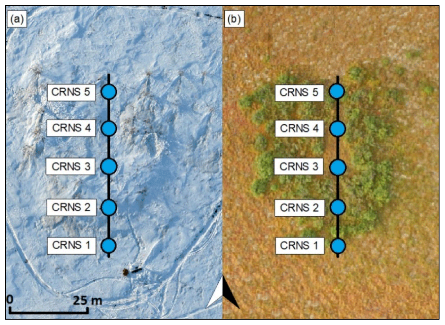
Figure 3CRNS transect at Trail Valley Creek during the 2016/2017 and 2017/2018 field seasons. (a) Site transect during winter sampling. (b) Site during snow-free conditions; this image displays the tall alder shrub vegetation (green) and tundra vegetation (orange).
Each sensor tube is the same size and style as shown in Fig. 2b.
3.3 CRNS parameters
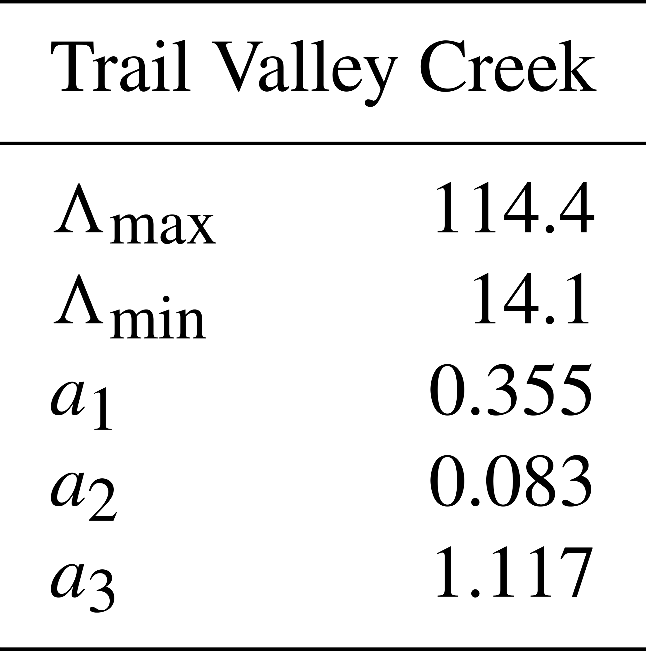
The standard terrestrial parameters (Table 1) were used for the Elora study site. However, the TVC snow cover is underlain by a high-porosity soil matrix with an active layer thickness of 0.5 to 1.0 m (Wilcox et al., 2019), and this active layer is typically saturated with liquid water prior to freeze up and therefore has a high ice content during the winter season (Wrona, 2016). As a result, we applied the manufacturer-suggested glacier parameters (Table 2) to this Arctic site. However, we increased the a1 parameter in order to create a site-specific calibration which addressed the factor that the TVC subsurface was not pure water/ice but had mineral and organic properties and was highly porous and permeable – typical of an Arctic landscape. We used a systematic approach on each of the parameters and observed a significant increase in data quality, relative to field measurements, when adjusting only the a1 parameter. Howat et al. (2018) and Gugerli et al. (2019) tested a similar CRNS model on the Greenland Ice Sheet and the Glacier de la Plaine Morte in Switzerland, and they were successful using the manufacturer-provided glacier parameters. Although they tested a non-invasive CRNS model, findings from Schattan et al. (2017), Schrön et al. (2017), and Wallbank et al. (2021) suggest that adjusting the fitting parameters may lead to improved results, and in discussion with the manufacturer, it was confirmed that adjusting the fitting parameters for this grounded in situ CRNS model may also lead to improved results. Future research is recommended to investigate the impact of each parameter and to explore the potential of a standard set of factory-fitting parameters for an Arctic landscape.
Table 1Factory-fitting parameters for Eq. (5) were used for the Elora site. Values were obtained from the CRNS manufacturer and are representative of a terrestrial landscape.
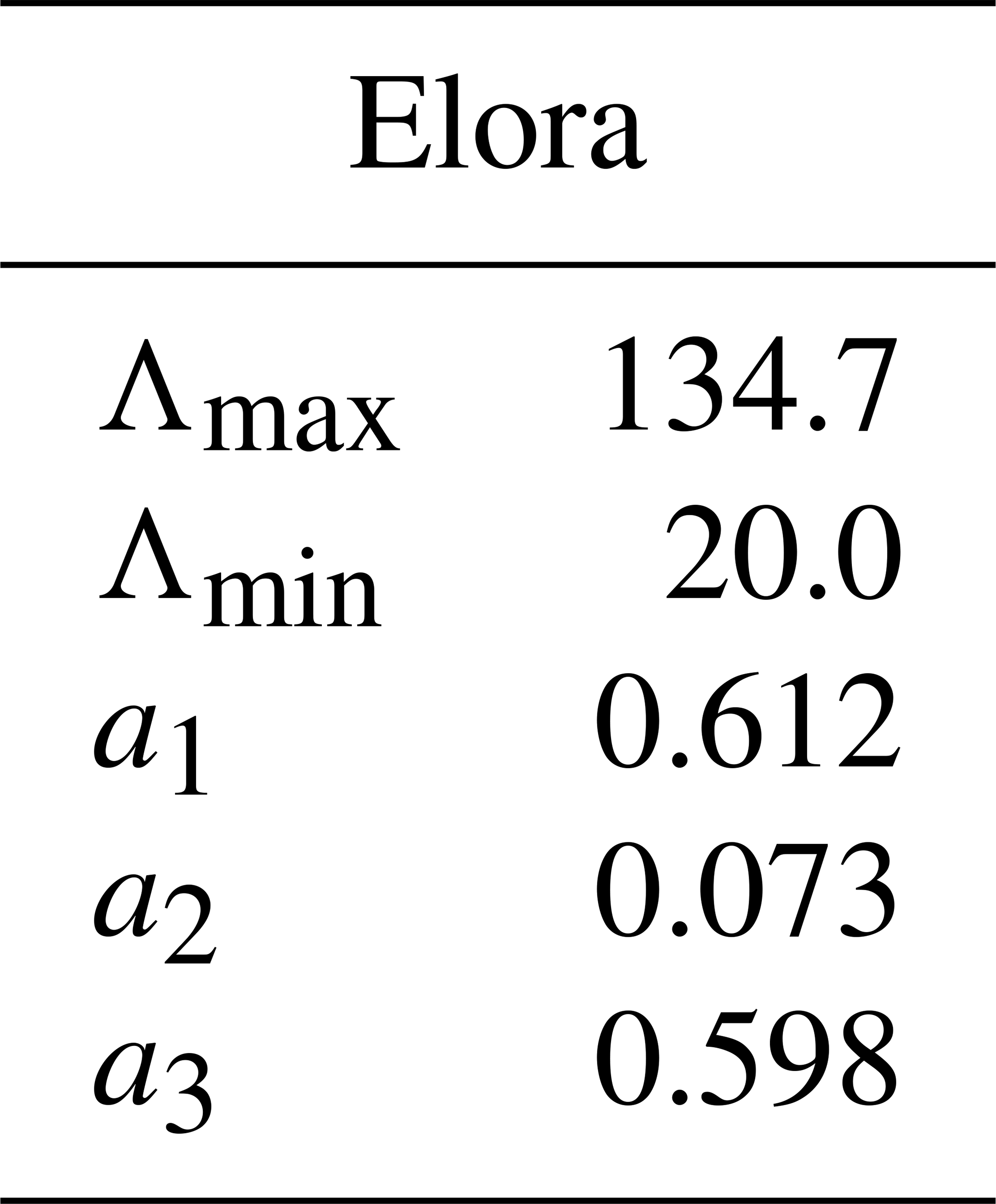
Table 2Factory-fitting parameters used for Eq. (5) for the Trail Valley Creek shrub site. Values were obtained from the CRNS manufacturer and are representative of a glacier landscape. The a1 parameter was adjusted from 0.313 to 0.355 to represent the high-porosity, saturated soils of the study site.
3.4 Snow surveys
A total of five snow surveys were conducted at the Elora site during accumulation and melt conditions from 11 February to 14 March 2017, as well as 11 surveys from 23 December 2017 to 20 February 2018. The snow surveys consisted of a snow-core campaign utilizing an ESC30-style snow corer from Snow-Hydro which features a cross-sectional area of 30 cm2 for measuring snow depth and density. The snow cores were transferred to a plastic bag and weighed on-site with an electronic scale (A&D HT-3000). The depth and density of each snow sample were recorded and used to calculate the SWE. Snow surveys at this site consisted of three to four snow core samples taken within a 1 m proximity to the CRNS. Snow core results were averaged to represent a single value for that date. Results from Turcan and Loijens (1975), Peterson and Brown (1975), Goodison et al. (1981), Sturm et al. (2010), and Royer et al. (2021) state that the standard measurement error associated with using this type of snow corer ranges from 1 %–10 %.
Snow surveys were performed at the TVC site during the 2016/2017 winter season from 13 December 2016 to 6 June 2017 and 28 April 2018 to 7 June 2018 during the 2017/2018 season. A total of 17 surveys were conducted in 2016/2017 and 28 in the 2017/2018 winter season. The snow-core campaign included accumulation and snowmelt conditions and consisted of 10 measurements (approximately equally spaced apart) along the 50 m transect (Fig. 3). Again, a Snow-Hydro snow corer was used. Using the same approach as the Elora site, samples had their depth and weight recorded immediately after collection and were used to calculate SWE. Data from this site were used in two ways:
-
SWE calculated from the five CRNS instruments was averaged, and this single averaged value was used to represent the total snowdrift for that date.
-
SWE calculated for each CRNS was compared with the snow survey measurement obtained nearest to the specific CRNS of interest. This allowed the CRNSs to be compared to one another within the snowdrift over the course of the snow-covered season.
4.1 Relationship between neutron counts and SWE
Corrected, moderated neutron counts, N from Eq. (1) (simply referred to as counts, or neutron counts, for the remainder of the paper), were assessed in relation to SWE. The Elora dataset was tested according to Eq. (4) and additional linear regression, whereas the TVC dataset SWE was derived utilizing Eq. (4) only because the deeper snowpack there means the linearity between SWE and neutron counts no longer holds.
The relationship between neutron counts and SWE at Elora was assessed in two ways. First, the N0-calibration function (Eqs. 4 and 5) was used to estimate SWE from the neutron counts and compared to snow survey measurements of SWE. Using this approach, the R2 was 0.74 when combining data from the winters of 2016 and 2017 (Fig. 4), and it improved to 0.93 with the exclusion of an outlier from the 2017/2018 dataset.
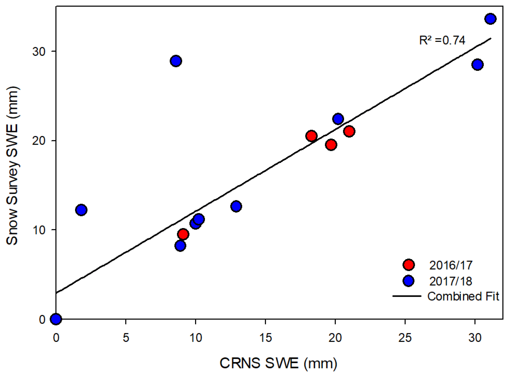
Figure 4Snow survey SWE vs. CRNS-estimated SWE at Elora during both winter seasons. Outlier from 2017/2018 is outlined.
Second, we carried out a bivariate analysis directly between neutron counts and SWE from the snow surveys using a linear regression (Fig. 5a). Although the N0-calibration function (Eqs. 4 and 5) is commonly utilized due to the nonlinearity of the cosmic ray attenuation method, the manufacturer notes that a linear approximation may have potential to be effectively utilized for a grounded in situ CRNS up to 150 mm of SWE. Past this value, the nonlinearity of the N0-calibration function becomes more pronounced (Fig. A1) and should be accounted for. Additionally, although they tested a different CRNS model, findings from Sigouin and Si (2016) and Bogena et al. (2020) state that the linear regression methodology is able to determine the SWE of the snowpack reasonably well.
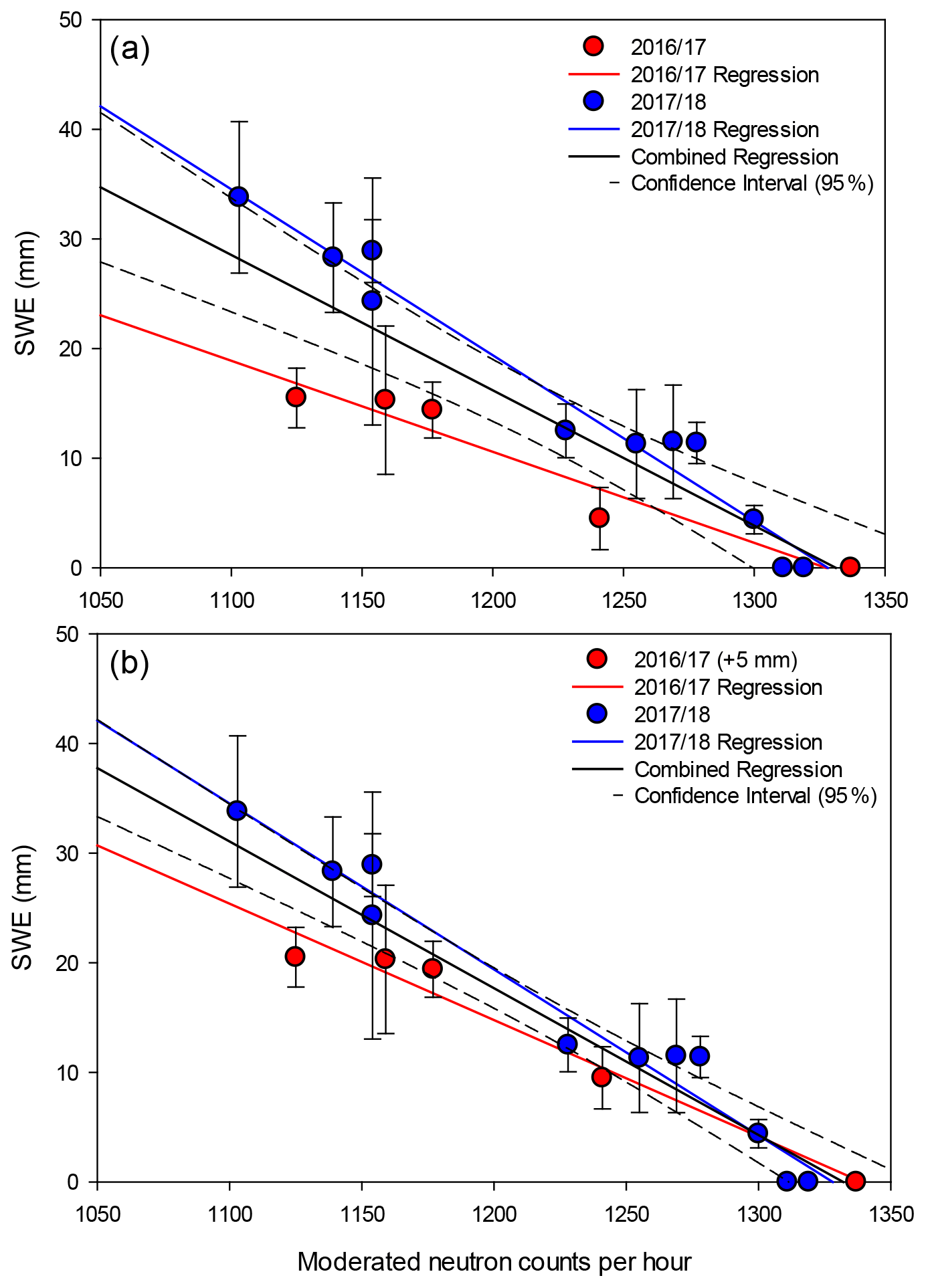
Figure 5Comparison between counts (N) and average snow survey SWE at the Elora site. Panel (a) shows both 2016/2017 and 2017/2018, with red and blue lines showing the regression Eqs. (6) and (7). Panel (b) shows 2016/2017 and 2017/2018 but with the regression equation for 2016/2017 SWE values adjusted to account for the antecedent water content in the top few centimeters of soil. The red line represents Eq. (7) and blue Eq. (8). Zero SWE values represent snow-free conditions, and the error bars represent the standard deviations.
Utilizing this approach provided a best-fit linear regression that varied between each study year as follows:
and
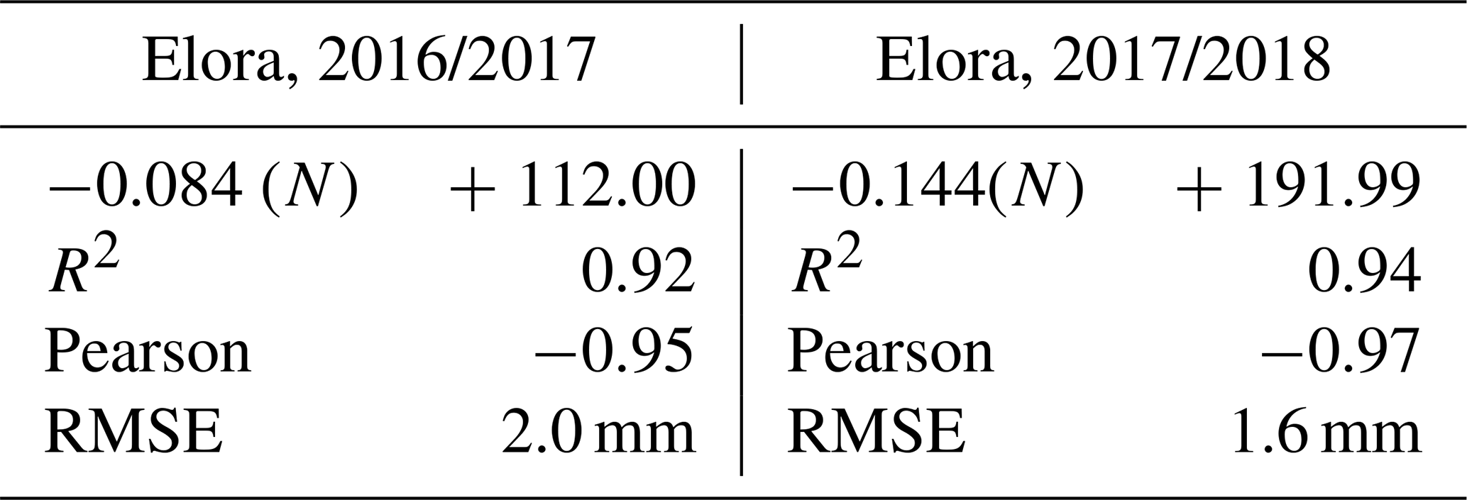
where N is the 12 h averaged counts (N) from Eq. (1) which has already been normalized by the snow-free near-surface water content from Eq. (4). The statistical analysis (Table 3) suggests a strong correlation to the linear regression equations and indicates a high probability of predicting future responses, suggesting that the linear regression equations may well be transferable in time. The RMSE of the CRNS-measured maximum SWE was exceptionally low: 2.0 mm in 2016/2017 and 1.6 mm in 2017/2018.
Table 3Statistical analysis summary of the Elora linear regressions.
However, the slope and y-intercept values for 2016 vs. 2017 (Eqs. 6 and 7) are considerably different. The discrepancy in the y intercept is believed to be related to the CRNS being installed later in the winter season in 2016/2017 (11 February 2017) after the first accumulation of snow at the site. As a result, the sensors neutron count baseline does not incorporate the near-surface water content prior to the initial winter freeze-up and therefore, based on Eq. (4), underrepresents the actual SWE at this site. The majority of this unaccounted water content is likely stored in the first few centimeters of soil. In 2017/2018, however, the CRNS was installed on 4 December 2017, before the first accumulation of snow on the ground and the initial soil freeze-up. This means the CRNSs' baselines between the two seasons are likely to be different. To consider if this explanation is reasonable, we followed the approach of Sigouin and Si (2016), also noted by Royer et al. (2021), in which the authors applied a correction based on soil water storage in the top 10 cm of the soil profile and adjusted their SWE values accordingly. To follow this approach, we used an estimated water capacity of the top 10 cm soil layer to be up to 2 mm cm−1 (Blencowe et al., 1960; Ball, 2001) and assumed a 50 % soil moisture. This provided an estimated soil water storage of up to 5 mm. Adding this value to the non-zero SWE from snow surveys conducted in 2016/2017 and conducting a second regression to the 2016/2017 data provided a best-fit equation of
As shown in Fig. 5b, this adjusted equation provides a slope and y intercept that are closer to those of the 2017/2018 equation (Eq. 7). This illustrates the significance of installing the CRNS prior to the start of the snow-covered season. However, due to this late season installation, we were able to reasonably estimate the antecedent soil water capacity by comparing the regression trend lines from year to year. This comparison between snow seasons is possible because the soil water storage directly impacts the N0 value (or N when SWE is zero). In practice, this further indicates that a linear regression function is well transferable in time at sites with similar soil water storage capacity – such as Elora. In a broader approach, this allows researchers and operators to set up the CRNS, even after the initial snowfall and subsequent soil freeze-up, and capture accurate SWE data so long as it is corrected for soil moisture conditions afterwards (Royer et al., 2021). Additionally, another significant advantage of utilizing a linear regression approach is that it is considerably more time efficient than fitting the full N0-calibration function.
This approach is most practical for cosmic ray neutron attenuation up to ∼150 mm of SWE; past this point, the nonlinearity of the effective attenuation length vs. SWE (Eq. 5) becomes more pronounced. Considering that the maximum SWE for both winter seasons at Elora was well below 150 mm, the linear regression approach provided reasonably accurate results. Bogena et al. (2020) note that, to date, there is no consensus on which single method is best suited to convert neutron intensity data into SWE. This section demonstrates that a grounded in situ CRNS utilizing a linear regression approach is able to reasonably measure SWE. Future research is recommended to assess the linear regression analysis vs. the nonlinear approach in order to quantify the measurement accuracy discrepancy between the two approaches at low, moderate, and high-SWE sites using grounded in situ CRNS. Considering that the grounded in situ CRNS requires virtually zero maintenance and can be set up by one person in under an hour, the regression equation methodology may be an effective approach for quickly estimating SWE at remote sites and at sites where soil moisture is rather consistent.
4.2 Temporal snow cover development and melt
Using Eq. (4), the CRNS instrument allowed for the continuous measurement of SWE over an entire winter accumulation and melt season at one point at the Elora site and for multiple sites across the TVC snow drift. Figure 6 shows changes in SWE at the Elora site for both study years and illustrates the potential for the CRNS approach to measure key aspects of the winter SWE, including maximum SWE, rapid changes in SWE due to both snowfall accumulation and snowmelt, and the timing of snowpack removal due to melt. For example, during the 2016/2017 winter season the maximum SWE peaked briefly at 31 mm in mid-February and 42 mm in late January 2017/2018 (Fig. 6) and then rapidly decreased over the next few days due to snowmelt. Measuring such rapid changes in SWE would be very challenging using manual snow survey measurements, and only a few other instruments, such as gamma snow sensors, can achieve this type of high-temporal-resolution, point SWE observations. The CRNS also shows that in 2016/2017, the site became snow-free numerous times over the winter (Fig. 6), and the snow cover was removed for the last time on 14 March. In 2017/2018 there was a continuous snow cover from December to late January, and the snow cover was then removed on 20 February and did not form again that winter. The small, short duration fluctuations in SWE in both years (Fig. 6) likely represent the periods of snowfall, snowmelt, sublimation, and wind erosion/transport. In addition, small fluctuations are likely also due to the inherent measurement error of the CRNS. This error has yet to be definitively quantified but is assumed to average below 7 % (Kodama et al., 1979; Howat et al., 2018; Gugerli et al., 2019). Figure 6, at some intervals, shows negative SWE during both winters, and this implies that the CRNS is recording a higher number of counts (N) than was originally measured during its baseline (N0), meaning that the CRNS is sensing a lower amount of near-surface water content than was recorded at the start of the winter season. This is directly due to the CRNS fundamental measurement basis in which any deviations from the baseline counting rate are inversely proportional to the amount of near-surface water content (Eq. 4). In these cases, the negative values imply that the snow has melted and infiltrated past the measurement scope of the CRNS, and therefore the immediate surrounding environment is drier than it was just before the onset of the winter season's first snowfall and initial soil freeze-up.
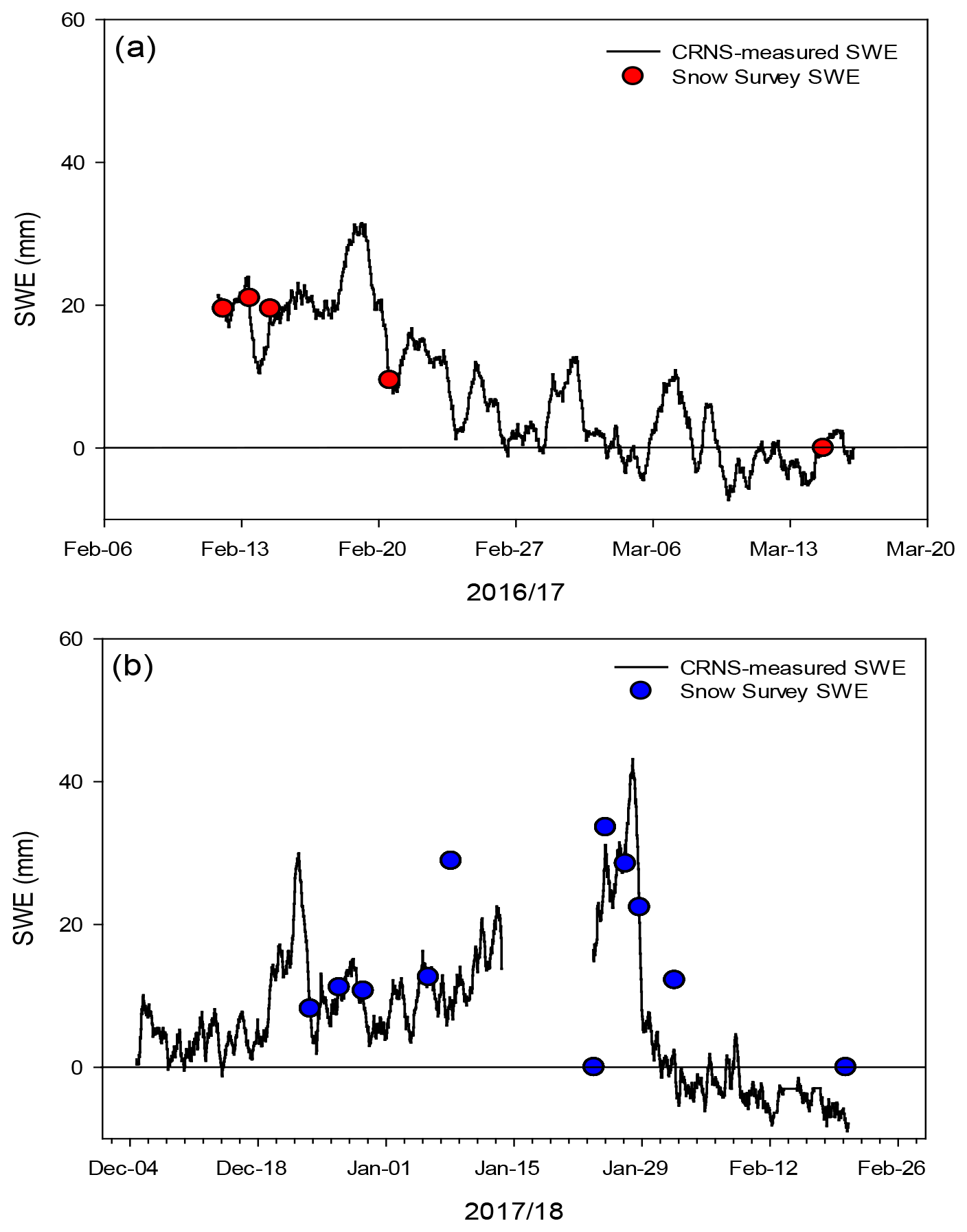
Figure 6Continuous measurement of SWE at the low-SWE Elora site during the (a) 2016/2017 and (b) 2017/2018 winter seasons. When SWE values are negative, the CRNS is recording a lower near-surface water content than its baseline. CRNS SWE values were calculated using Eq. (4).
One example of the advantage of using a CRNS system is shown during 2017/2018 (Fig. 6b) when there was a notable discrepancy on 23 January 2018 between the observed and estimated SWE. The CRNS estimated 16 mm of SWE, while the snow survey conducted on the same day resulted in a SWE of 0 mm. This discrepancy occurred because a warm spell led to rapid snowmelt between 21 and 22 January, immediately followed by a return to below-freezing temperatures. This resulted in the formation of a thick ice layer covering the site, which the snow survey was not able to measure. However, the CRNS was able to record the SWE of this ice layer.
Figure 7 shows a similar time series for SWE at the TVC site. In this example, the SWEs from the five CRNS instruments were estimated using Eq. (4), averaged to represent a single value, and compared to snow survey data across the same transect. The initial snow-precipitation events of the 2016/2017 season occurred in late November 2017 but a month earlier in 2017/2018. During both years, SWE continued to increase for the remainder of the winter. Unlike the Elora site, there were no midwinter melt events, but the small decreases in SWE are likely due to removal of snow from the transect by blowing snow erosion. The maximum average SWE across the transect in 2016/2017 was 370 mm. Peak SWE occurred on 9 May, a few weeks prior to the onset of snowmelt. Small, high-frequency SWE fluctuations during this period are primarily due to the change in the sampling rate of the CRNS. This change occurred when we switched the CRNS system from winter power conservation mode, for which the sampling rate was four 1 h interval recordings per day, to the default sampling rate, which was twenty-four 1 h interval recordings per day. The maximum SWE at TVC in the 2017/2018 season was 369 mm (13 May), and once again, it occurred shortly prior to the initial onset of the spring snowmelt. Since the CRNS system measures total SWE (including liquid water within the snowpack), it does not identify when surface snowmelt begins but instead detects when meltwater begins to leave the base of the snowpack and SWE begins to decline. This ability allows for the direct measurement of snowmelt runoff from the snow cover and is an exceptionally useful parameter for studying snowmelt runoff and for testing the performance of snow models used for modeling snowmelt runoff.

Figure 7Continuous measurement of a snowdrift at TVC in the (a) 2016/2017 and (b) 2017/2018 winter seasons. CRNS-measured SWE was averaged from the five CRNSs, and values were calculated using Eq. (4).
4.3 Snow accumulation and melt at locations across a snow drift
Figure 8 shows snow accumulation and melt at each of the five CRNSs across the TVC drift (Fig. 3). In the winter of 2016/2017 (Fig. 8a), the snow drift began to form in the center of the shrub patch in early December, while significant accumulation did not begin on the southern edge of the patch until a few weeks later. Over the rest of the winter, the snow cover in the center of the shrub patch (CRNS 3 and 4) continued to accumulate rapidly as blowing snow was deposited in the drift, and these sites ended up with the largest SWE at the end of winter. In this case, the center of the patch had 555 mm of SWE at the end of winter in 2016/2017 and 645 mm at the end of winter in 2017/2018. Other parts of the shrub patch also had similar maximum SWE values in comparison to one another from both years (Figs. 8a and b). As described earlier, the noisiness shown in Fig. 8 is due to a change in frequency of the sampling rate.
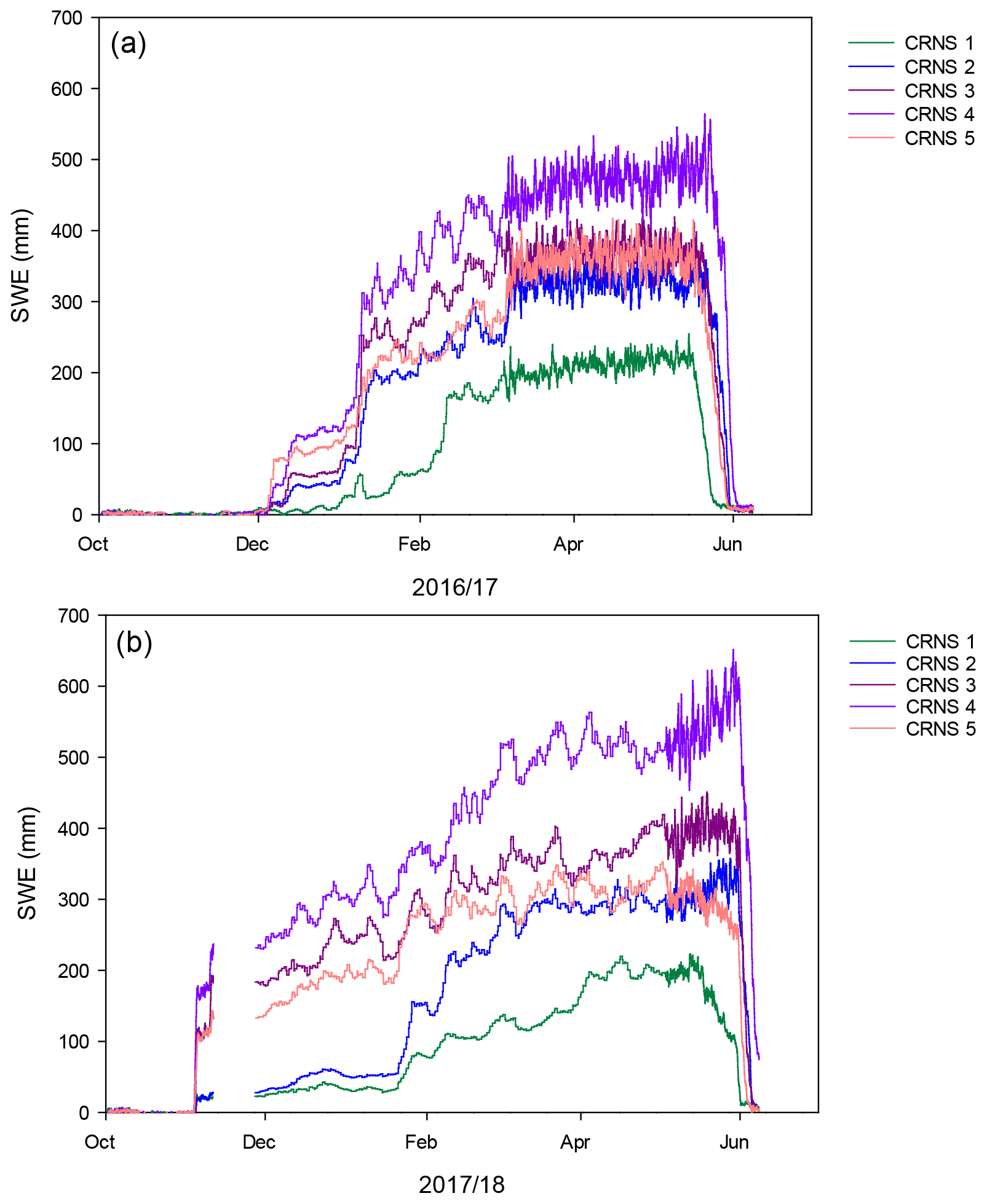
Figure 8Change in SWE at TVC from each CRNS throughout the (a) 2016/2017 and (b) 2017/2018 winter seasons. CRNS 1 and 5 are located at the edges of the shrub patch, and CRNS 2 to 4 are located in the center of the patch.
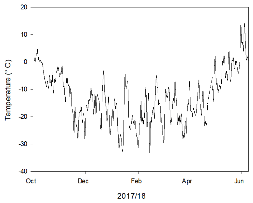
Spring snowmelt begins in mid-May at TVC; however, the early season melt is likely retained within the snowpack as liquid water is refrozen into ice (Wrona, 2016). Early spring snowmelt, primarily from the snowpack surface or near-surface, is known to refreeze during infiltration of deep snowpacks (Pomeroy and Gray, 1995; Marsh and Pomeroy, 1996), and this infiltration refreeze is amplified when temperatures fluctuate between freezing and above freezing – as is common during spring snowmelt. Temperature data from 2017/2018 (Fig. B1) confirm that early spring temperatures tended to fluctuate between freezing and above freezing. Early into the spring season snow-core campaign, we visually noticed the snowpack surface and near-surface melting and, later in the season, noticed distinct variability in the amount of water saturation within the snow cores on different days. After sufficient melt and subsequent snowpack saturation, water is available to infiltrate the soil or runoff laterally (Quinton et al., 2010), and it is likely that at this point the melt began to exit the measurement footprint of the grounded in situ CRNS and led to the rapid decrease in SWE (Fig. 8a).
Loss of SWE begins first at CRNS 1 (16 May) at the edge of the shrub patch where the snow is shallower. As melt progressed, snow mass is removed from each location in the following order: CRNS 5 on 17 May, CRNS 2 and 3 on 20 May, and lastly, CRNS 4 on 23 May. By 7 June, all five CRNSs indicated that the snow overlying them had melted. In both seasons, CRNS 5 accumulated a higher SWE than CRNS 2 (Figs. 8a and b) but began to melt days earlier. At the same time, as CRNS 5 is melting, CRNS 2, 4, and, to a lesser extent, CRNS 3 experienced a slight increase in SWE, likely attributed to a lateral redistribution of snowmelt from the margin of the shrub site (CRNS 5) to the interior of the patch (CRNS 2, 3, 4). Using these changes in SWE from the CRNSs provides continuous detailed snow accumulation and melt across a snowdrift for a complete winter season. This type of unique dataset can be expanded and would be particularly useful for prominent snowdrifts or features. For example, a significant snowdrift in a known watershed at critical locations along several margin points and semi-margin points, as well as in the relative center, would allow for the collection of continuous data regarding the rate of accumulation, melt, and snow transport (e.g., due to blowing snow) with essentially no maintenance and minimal user operation – ideal for certain water resource management applications.
Grounded in situ CRNSs were tested at a temperate low-SWE agricultural field in Elora, Ontario, and high-SWE Arctic tundra site in Trail Valley Creek, Northwest Territories. A strong negative correlation was found between the counts and the manual SWE measurements obtained from snow surveying. The relationship implies that when SWE increases, the moderated neutron counts decrease. An empirical equation for estimating SWE at the Elora site appeared to indicate that low-SWE sites with similar annual soil water storage may provide reasonable SWE accuracy and are well transferable in time. Additionally, the comparison of annual regression trend lines at a single site may be used to reasonably estimate soil water storage. This allows researchers and operators to set up the CRNS, even after the initial snowfall and subsequent soil freeze-up, and capture accurate SWE data so long as it is corrected for soil moisture conditions afterwards. Another significant advantage of utilizing a linear regression approach is that it is considerably more time efficient than fitting the full N0-calibration function but limited to SWE <150 mm.
By applying five CRNS units in a transect, we were able to obtain continuous accumulation and melt data for a single snow feature, including a comparison of accumulation and melt within the snowdrift itself. We were able to determine the exact date of the peak SWE and of the onset, and completion, of snowmelt. The transect data appeared to indicate that blowing snow and lateral redistribution of meltwater through infiltration have a considerable influence on Arctic snowdrifts; however, further research is needed to quantify the impact of each process. Future research is recommended to assess the linear regression analysis vs. the nonlinear formulation to quantify the measurement accuracy discrepancy between the two approaches at low, moderate, and high-SWE sites using grounded in situ CRNS.
A unique advantage of CRNS systems is that ice layers and wet snow from mid-winter melt events do not impact the sensor measurement accuracy, and the CRNS measures all components of the snowpack SWE, including dry snow, ice layers, and wet snow. Using a CRNS for monitoring SWE provides a unique ability to continuously measure SWE, and these systems can be installed in remote locations and in areas where performing regularly scheduled manual measurements is costly and logistically impractical. As such, the CRNS system replaces the need of manually conducting snow surveys and requires virtually zero operational maintenance.
Since it was found that soil water in the top soil profile directly surrounding the CRNS affected the neutron intensity, future research involving a CRNS should examine at what soil depth the CRNS is impacted by soil water content or, alternatively, could be installed so that meltwater infiltration is shallow enough that water does not infiltrate past the base of the sensor. Additionally, we noted that the terrestrial set of parameters appeared to record low-SWE environments exceptionally well; however, the glacier set of calibration parameters appeared to have some flexibility. This seems to indicate that site-specific calibration may not apply only to the conventional parameters, such as the snow-free moderated neutron count (N0), but also to the CRNS fitting parameters. Future research is recommended to investigate the impact of each factory-fitting parameter and to explore the potential of a standard set of factory-fitting parameters for an Arctic landscape. SWE data from the CRNS could be used for validating surface mass balance models, verifying remote sensing approaches, and for better understanding the effects of a changing climate on snowfall, mid-winter thaws, blowing snow, expanding shrubs capturing blowing snow, spatial variability in snow depth and snow water equivalent (SWE), and the rate of spring melt – all of which are poorly known. Future works are recommended to utilize grounded in situ CRNS in a transect for a significant snowdrift by incorporating a CRNS unit at critical locations along several margin and semi-margin points, as well as in the relative center, to allow for the collection of continuous data in vital watersheds for water resource management applications.

Data for this paper will be available at https://doi.org/10.5683/SP3/ODZIXX.
AJ and PM conceived the idea of this work. AJ performed the investigations and analysis, collected the field data, interpreted the data results, and wrote the manuscript. PM is the principal co-author and contributed to the ideas, investigation, and analysis, as well as writing and editing of the manuscript. BW reviewed the manuscript and provided support related to logistics and fieldwork. DD assisted with troubleshooting the CRNS instruments and formulated the instrument factory-fitting parameters.
Some authors are members of the editorial board of The Cryosphere. The peer-review process was guided by an independent editor, and the authors have also no other competing interests to declare.
Publisher’s note: Copernicus Publications remains neutral with regard to jurisdictional claims in published maps and institutional affiliations.
Funding and logistical support for this study was provided by the Canada Research Chairs program, Wilfrid Laurier University, the Natural Science and Engineering Research Council, Polar Knowledge Canada, Arctic Net, and the Polar Continental Shelf Program. This project was completed with approval from the Government of the Northwest Territories and the Aurora Research Institute under Science License no. 16047 and 16237. The authors sincerely thank Matthew Tsui, Barun Majumder, Brampton Dakin, Philip Mann, and Aaron Berg. We sincerely thank our anonymous reviewers and the community reviewer, Alain Royer.
This paper was edited by Melody Sandells and reviewed by two anonymous referees.
Ball, J.: Soil and water relationships, Noble Research Institute, available at: https://www.noble.org/news/publications/ (last access: 15 October 2021), 2001.
Bartol, J.: Listening for cosmic rays, Based upon report number 5 of the scientific report series of the Aurora Research Institute, Aurora College, Inuvik, NWT, Canada, 1999.
Blencowe, J., Moore, S., Young, G., Shearer, R. Hagerstrom, R., Conley W., and Potter, J.: U.S. Soil Department of Agriculture, 462, Washington, DC, USA, 1960.
Bogena, H., Herrmann, F., Jakobi, J., Brogi, C., Ilias, A., Huisman, A., Panagopoulos, A., and Pisinaras V.: Monitoring of snowpack dynamics with cosmic-ray neutron probes: a comparison of four conversion methods, Front. Water, 2, 19, https://doi.org/10.3389/frwa.2020.00019, 2020.
Bush, E. and Lemmen, D.: Canada's changing climate report, Government of Canada, Ottawa, Ontario, 444 pp., 2019.
Chrisman, B. and Zreda, M.: Quantifying mesoscale soil moisture with the cosmic-ray rover, Hydrol. Earth Syst. Sci., 17, 5097–5108, https://doi.org/10.5194/hess-17-5097-2013, 2013.
Deems, J., Painter, T., and Finnegan, D.: Lidar measurement of snow depth: a review, J. Glaciol., 59, 215, https://doi.org/10.3189/2013JoG12J154, 2013.
Delunel, R., Bourles, D., van der Beek, P., Schlunegger, F., Leya, I., Masarik, J., and Paquet, E.: Snow shielding factors for cosmogenic nuclide dating inferred from long-term neutron detector monitoring, Quat. Geochronol., 24, 6–24, 2014.
Derksen, C. and Brown, R.: Spring snow cover extent reductions in the 2008-2012 period exceeding climate model projections, Geophys. Res. Lett., 39, L19504, https://doi.org/10.1029/2012GL053387, 2012.
Derksen, C., Xu, X., Dunbar, S., Colliander, A., Kim, Y., Kimball, J., Black, A., Euskirchen, E., Langlois, A., Loranty, M., Marsh, P., Rautianen, K., Roy, A., Royer, A., and Stephens, J.: Retrieving landscape freeze/thaw state from Soil Moisture Active Passive (SMAP) radar and radiometer measurements, Remote Sens. Environ., 194, 48–62, 2017.
Desilets, D.: Intensity correction factors for a cosmic ray neutron sensor, Hydroinnova Technical Document, 21–01, 1–12, https://doi.org/10.5281/zenodo.4569062, 2021.
Desilets, D., Zreda, M., and Ferré, A.: Nature's neutron probe: Land surface hydrology at an elusive scale with cosmic rays, Water Resour. Res., 46, W11505, https://doi.org/10.1029/2009WR008726, 2010.
Goodison, B., Ferguson, H., and McKay, G.: Measurement and data analysis, in handbook of snow: principles, processes, management, and use, Pergamon press Canada, Toronto, Canada, 191–274, ISBN 978 0 080 25374 9, 1981.
Goodsite, M., Bertelsen, R., Pertoldi-Bianchi, S., Ren, J., Watt, L., and Johannsson, H.: The role of science diplomacy: a historical development and international legal framework of arctic research stations under conditions of climate change, post-cold war geopolitics and globalization/power transition, Journal of Environmental Studies and Sciences, 6, 645–661, 2016.
Gray, D., Erickson, D., and Abbey, F.: Energy studies in an arctic environment, Report No. 74–18, Environmental Social Committee, Northern Pipelines Task Force on Northern Oil Development, Information Canada, Cat. No. R57-10/1974, Ottawa, 60 pp., 1974.
Gray, D., Pomeroy, J., and Granger, R.: Modelling snow transport, snowmelt and meltwater infiltration in open, northern regions, Division of Hydrology, University of Saskatchewan, Saskatoon, Saskatchewan, Canada, 1989.
Gugerli, R., Salzmann, N., Huss, M., and Desilets, D.: Continuous and autonomous snow water equivalent measurements by a cosmic ray sensor on an alpine glacier, The Cryosphere, 13, 3413–3434, https://doi.org/10.5194/tc-13-3413-2019, 2019.
Hori, M., Sugiura, K., Kobayashi, K., Aoki, T., Tanikawa, T., Kuchiki, K., Niwano, M., and Enomoto, H.: A 38-years (1978–2015) northern hemisphere daily snow cover extent product derived using consistent objective criteria from satellite-borne optical sensors, Remote Sens. Environ., 191, 402–418, 2017.
Howat, I. M., de la Peña, S., Desilets, D., and Womack, G.: Autonomous ice sheet surface mass balance measurements from cosmic rays, The Cryosphere, 12, 2099–2108, https://doi.org/10.5194/tc-12-2099-2018, 2018.
Kinar, N. and Pomeroy, J.: Measurement of the physical properties of the snowpack, Rev. Geophys., 53, 481–544, https://doi.org/10.1002/2015RG000481, 2015.
Kirkham, D., Koch, I., Saloranta, T., Litt, M., Stigter, E., Møen, K., Thapa, A., Kjetil, M., and Immerzeel, W.: Near Real-Time Measurement of Snow Water Equivalent in the Nepal Himalayas, Front. Earth Sci., 7, 177, https://doi.org/10.3389/feart.2019.00177, 2019.
Klein, K. L., Steigies, C., Wimmer-Schweingruber, R. F., Kudela, K., Strharsky, I., Langer, R., Usoskin, I., Ibragimov, A., Flückiger, E. O., Bütikofer, R., Eroshenko, E., Belov, A., Yanke, V., Fuller, N., Mavromichalaki, H., Papaioannou, A., Sarlanis, C., Souvatzoglou, G., Plainaki, C., Geron-Tidou, M., Papailiou, M., Mariatos, G., Chilingaryan, A., Hovsepyan, G., Reymers, A., Parisi, M., Kryakunova, O., Tsepakina, I., Nikolayevskiy, N., Dor-Man, L., Pustil’Nik, L., and García-Población, O.: The real-time neutron monitor database, COSPAR Scientific Assembly, Bremen, Germany, https://www.nmdb.eu/nest/ (last access: 1 October 2020), 2010.
Koch, F., Henkel, P., Appel, F., Schmid, L., Bach, H., Lamn, M., Prasch, M., Schweizer, J., and Mauser, W.: Retrieval of snow water equivalent, liquid water content and snow height of dry and wet snow by combining GPS signal attenuation and time delay, Water Resour. Res., 55, 4465–4487, https://doi.org/10.1029/2018WR024431, 2019.
Kodama, M., Nakai, K., Kawasaki, S., and Wada, M.: An application of cosmic-ray neutron measurements to the determination of the snow-water equivalent, J. Hydrol., 41, 85–92, 1979.
Kuwabara, T., Bieber, J.W., Clem, J., Evenson, P., and Pyle, R.: Development of a ground level enhancement system based upon neutron monitors, Space Weather, 4, 1542–7390, https://doi.org/10.1029/2006SW000223, 2006.
Marsh, P. and Pomeroy J. W.: Meltwater fluxes at an arctic forest-tundra site, Hydrol. Process., 10, 1383–1400, 1996.
Marsh, P. and Woo, M.: Snowmelt, glacier melt, and high arctic streamflow regimes, Can. J. Earth Sci., 18, 1380–1384, 1981.
Pan, X., Yang, D., Li, Y., Barr, A., Helgason, W., Hayashi, M., Marsh, P., Pomeroy, J., and Janowicz, R. J.: Bias corrections of precipitation measurements across experimental sites in different ecoclimatic regions of western Canada, The Cryosphere, 10, 2347–2360, https://doi.org/10.5194/tc-10-2347-2016, 2016.
Paquet, E. and Laval, M.: Feedback and prospects for operating the EDF cosmic-radiation snow sensors, Houille Blanche, 2, 113–119, https://doi.org/10.1051/lhb:200602015, 2005
Paquet, E., Laval, M., Basaleaev, M., Belov, A., Eroshenko, E., Kartyshov, V., Struminsky, A., and Yanke, V.: An application of cosmic-ray neutron measurements to the determination of the snow water equivalent, Proceedings of the 30th International Cosmic Ray Conference, Mexico City, Mexico, 1, 761–764, 2008.
Peterson, N. and Brown, J.: Accuracy of snow measurements, in: Proceedings of the 43rd Annual Meeting of the Western Snow Conference, Coronado, California, 1–5, 1975.
Pomeroy, J. and Gray, D.: Snowcover: Accumulation, relocation and management, NHRI Science Report No. 7, 1995.
Quinton, W. and Marsh, P.: Image analysis and water tracing methods for examining runoff pathways, soil properties and residence times in the continuous permafrost zone, IAHS-AISH Publication, 258, 257–264, 1999.
Quinton, W., Hayashi, M., and Chasmer, L.: Permafrost-thaw-induced land-cover change in the Canadian subarctic: implications for water resources, Hydrol. Proc., 25, 152–158, https://doi.org/10.1002/hyp.7894, 2010.
Rees, A., English, M., Derksen, C., Toose, P., and Silis, A.: Observations of late winter Canadian tundra snow cover properties, Hydrol. Process., 28, 3962–3977, https://doi.org/10.1002/hyp.9931, 2014.
Royer, A., Roy, A., Jutras, S., and Langlois, A.: Review article: Performance assessment of electromagnetic wave-based field sensors for SWE monitoring, The Cryosphere Discuss. [preprint], https://doi.org/10.5194/tc-2021-163, in review, 2021.
Schattan, P., Baroni, G., Oswald, S., Schöber, J., Fey, C., Kormann, C., Huttenlau, M., and Achleitner S.: Continuous monitoring of snowpack dynamics in alpine terrain by aboveground neutron sensing, Water Resour. Res., 53, 3615–3634, https://doi.org/10.1002/2016WR020234, 2017.
Schattan, P., Köhli, M., Schrön, M., Baroni, G., and Oswald, S.: Sensing area-average snow water equivalent cosmic-ray neutrons: the influence of fractional snow cover, Water Resour. Res., 55, 10796–10812, 2019.
Schiermeier, Q.: Arctic stations need human touch, Nature, 441, 133, https://doi.org/10.1038/441133a, 2006.
Schrön, M., Köhli, M., Scheiffele, L., Iwema, J., Bogena, H. R., Lv, L., Martini, E., Baroni, G., Rosolem, R., Weimar, J., Mai, J., Cuntz, M., Rebmann, C., Oswald, S. E., Dietrich, P., Schmidt, U., and Zacharias, S.: Improving calibration and validation of cosmic-ray neutron sensors in the light of spatial sensitivity, Hydrol. Earth Syst. Sci., 21, 5009–5030, https://doi.org/10.5194/hess-21-5009-2017, 2017.
Sigouin, M. J. P. and Si, B. C.: Calibration of a non-invasive cosmic-ray probe for wide area snow water equivalent measurement, The Cryosphere, 10, 1181–1190, https://doi.org/10.5194/tc-10-1181-2016, 2016.
Stuefer, S., Kane, D. L., and Liston, G. E.: In situ snow water equivalent observations in the US arctic, Hydrol. Res., 44, 21–34, https://doi.org/10.2166/nh.2012.177, 2013.
Sturm, M., Liston, G. E., Benson, C. S., and Holmgren, J.: Characteristics and Growth of a Snowdrift in Arctic Alaska, U.S.A. Arct. Antarct. Alp. Res., 33, 319, https://doi.org/10.2307/1552239, 2001.
Sturm, M., Taras, B., Liston, G., Derksen, C., Jones, T., and Lea J.: Estimating snow water equivalent using snow depth data and climate classes, J. Hydrometeorol., 11, 1380–1394, 2010.
Tollefson, J.: Major report prompts warnings that the Arctic is unraveling, Nature, ISSN, 0028–0836, https://doi.org/10.1038/nature.2017.21911, 2017.
Turcan, J. and Loijens, J.: Accuracy of snow survey data and errors in snow sampler measurements, Proc. 32nd East. Snow. Conf., 2–11, 1975.
Walker, B., Wilcox, E. J., and Marsh, P.: Accuracy assessment of late winter snow depth mapping for tundra environments using Structure-from-Motion photogrammetry, Arctic Science, 7, 588-604, https://doi.org/10.1139/as-2020-0006, 2020.
Wallbank, J., Cole, S., Moore, R., Anderson, S., and Mellor, E.: Estimating snow water equivalent using cosmic-ray neutron sensors from the COSMOS-UK network, Hydrol. Proc., 35, 0885–6087, https://doi.org/10.1002/hyp.14048, 2021.
Wilcox, E. J., Keim, D., de Jong, T., Walker, B., Sonnentag, O., Sniderhan, A. E., Mann, P., and Marsh, P.: Tundra shrub expansion may amplify permafrost thaw by advancing snowmelt timing, Arctic Science, 5, 202–217, https://doi.org/10.1139/as-2018-0028, 2019.
Woolf, R., Sinclair, L., Brabant, R., Harvey, B., Phlips, B., Hutcheson, A., and Jackson, E.: Measurement of secondary cosmic-ray neutrons near the geomagnetic North Pole, J. Environ. Radioactiv., 198, 189–199, 2019.
Wrona, E.: Evaluation of novel remote sensing techniques for soil moisture monitoring in the Western Canadian Arctic, M. Sc., Thesis, University of Guelph, Canada, available at: http://hdl.handle.net/10214/10050 (last access: 1 September 2021), 2016.
Zreda, M., Shuttleworth, W. J., Zeng, X., Zweck, C., Desilets, D., Franz, T., and Rosolem, R.: COSMOS: the COsmic-ray Soil Moisture Observing System, Hydrol. Earth Syst. Sci., 16, 4079–4099, https://doi.org/10.5194/hess-16-4079-2012, 2012.