the Creative Commons Attribution 4.0 License.
the Creative Commons Attribution 4.0 License.
 | 22 Nov 2021
Two decades of dynamic change and progressive destabilization on the Thwaites Eastern Ice Shelf
Christian T. Wild
Adrian Luckman
Ted A. Scambos
Martin Truffer
Erin C. Pettit
Atsuhiro Muto
Bruce Wallin
Marin Klinger
Tyler Sutterley
Sarah F. Child
Cyrus Hulen
Jan T. M. Lenaerts
Michelle Maclennan
Eric Keenan
Devon Dunmire
The Thwaites Eastern Ice Shelf (TEIS) buttresses the eastern grounded portion of Thwaites Glacier through contact with a pinning point at its seaward limit. Loss of this ice shelf will promote further acceleration of Thwaites Glacier. Understanding the dynamic controls and structural integrity of the TEIS is therefore important to estimating Thwaites' future sea-level contribution. We present a ∼ 20-year record of change on the TEIS that reveals the dynamic controls governing the ice shelf's past behaviour and ongoing evolution. We derived ice velocities from MODIS and Sentinel-1 image data using feature tracking and speckle tracking, respectively, and we combined these records with ITS_LIVE and GOLIVE velocity products from Landsat-7 and Landsat-8. In addition, we estimated surface lowering and basal melt rates using the Reference Elevation Model of Antarctica (REMA) DEM in comparison to ICESat and ICESat-2 altimetry. Early in the record, TEIS flow dynamics were strongly controlled by the neighbouring Thwaites Western Ice Tongue (TWIT). Flow patterns on the TEIS changed following the disintegration of the TWIT around 2008, with a new divergence in ice flow developing around the pinning point at its seaward limit. Simultaneously, the TEIS developed new rifting that extends from the shear zone upstream of the ice rise and increased strain concentration within this shear zone. As these horizontal changes occurred, sustained thinning driven by basal melt reduced ice thickness, particularly near the grounding line and in the shear zone area upstream of the pinning point. This evidence of weakening at a rapid pace suggests that the TEIS is likely to fully destabilize in the next few decades, leading to further acceleration of Thwaites Glacier.
- Article
(11093 KB) - Full-text XML
- Companion paper
- BibTeX
- EndNote


Thwaites Glacier in West Antarctica holds the most important control on global sea-level rise over the next few centuries (Scambos et al., 2017). The broad causes and implications of the destabilization of Thwaites have been understood for decades: increased delivery of warm modified Circumpolar Deep Water (mCDW) to grounding zones triggers retreat of an ice sheet grounded well below sea level (e.g. Holland et al., 2019), leading to dynamic instability and greatly accelerated ice discharge into the ocean (Hughes, 1981; Mercer, 1978, Weertman, 1974). Recent evidence suggests that the predicted irreversible retreat of Thwaites Glacier is already underway (Joughin et al., 2014; Rignot et al., 2014). However, knowing the details of the timing, magnitude, and pace of the collapse of Thwaites are essential for more detailed forecasting of its sea-level contribution.
To understand these changes, we need to define both the oceanic forcing responsible for initiating retreat and the dynamic response that governs the inherent instability of the system. At the interface of this forcing and dynamic response are the floating ice components that form the seaward terminus of Thwaites Glacier. Because this ice interacts directly with ocean water, changes in its velocity and thickness may reveal clues about ocean forcing (e.g. MacGregor et al., 2012; Miles et al., 2020; Pritchard et al., 2012). Ice shelves and ice tongues also actively impact the dynamic stability of the system, as contact with the seafloor and embayment walls transmits backstress to grounded ice and slows ice flow and retreat (e.g. Dupont and Alley, 2005; MacGregor et al., 2012; Reese et al., 2017). Changes in ice-shelf dynamics and surface features may therefore signal fundamental imbalances in the system that can trigger rapid future change.

Figure 1Location map; the Thwaites Eastern Ice Shelf (TEIS) and Thwaites Western Ice Tongue (TWIT) are labelled. We also indicate the “pinning point,” the “shear zone” upstream of the pinning point, and the “shear margin” between the TEIS and the TWIT, which are terms discussed in the text. Three 5 km × 5 km sites of interest are shown, which are referred to in the text as the “grounding zone” (site 1), “mid-shelf” (site 2), and pinning point (site 3) areas. Data from these sites are shown in Figs. 2 and 5. Flowlines based on 2015–2020 velocities, labelled A and B, are represented in Hovmöller diagrams in Figs. 3 and 6. Grounding lines are from approximately 2000 (Rignot et al., 2016), 2004 (Bindschadler et al., 2011), 2011 (Rignot et al., 2016), and 2017 (Milillo et al., 2019). Figure created using the Antarctic Mapping Tools for MATLAB (Greene et al., 2017).
Thwaites Glacier has two floating ice areas: the Thwaites Western Ice Tongue (TWIT) and the Thwaites Eastern Ice Shelf (TEIS; Fig. 1). Most of the ice discharge from Thwaites passes through a fast-flowing channel that feeds the TWIT, which is an unconfined floating ice tongue that has largely disintegrated in recent years. Until the early 2000s, the TWIT was grounded on a subsea ridge near the ice edge (Rignot, 2001), which was likely the site of the main grounding line for this section of the ice shelf decades to centuries ago (Tinto and Bell, 2011). By 2009, the TWIT had largely lost contact with this pinning point (MacGregor et al., 2012; Tinto and Bell, 2011), although some grounding of the TWIT on the subsea ridge may have occurred intermittently for several more years (Miles et al., 2020).
Variability in TWIT velocity and structural integrity has been documented in detail (Miles et al., 2020; Mouginot et al., 2014). The last 20 years included periods of relatively stable velocity, which were accompanied by a strengthening of the shear margin between the TWIT and the TEIS. However, the more recent record has been dominated by periods of instability, with increasing velocities, extremely rapid ice-edge retreat, and a loss of coherence in the TWIT/TEIS shear margin (Miles et al., 2020; Mouginot et al., 2014). As the ice tongue nearly completely detached starting around 2008, the TWIT is unlikely to return to a stable configuration with a strong TWIT/TEIS shear margin.
The large changes observed on the TWIT have also significantly impacted the behaviour of the TEIS (Miles et al., 2020; Mouginot et al., 2014), which maintains a very different configuration than the TWIT. The same ridge that pinned the TWIT to the seafloor in past decades is responsible for a large ice rumple that confines the seaward limit of the TEIS (Tinto and Bell, 2011). As this ice rumple provides significant buttressing to the grounded ice upstream (Fürst et al., 2016; Reese et al., 2017), we will refer to it as a pinning point. This pinning point is at least partially responsible for the slower velocities and more stable calving-front positions of the TEIS as compared to the TWIT. The loss of this buttressing due to disintegration of the TEIS would therefore likely cause a step increase in ice discharge through the eastern portion of the ice stream, leading to ocean circulation changes and a response in the pace of grounding-line retreat.
In this study, we present detailed records from the last 2 decades of dynamic change on the TEIS. Patterns of ice-shelf speed, flow direction, and surface strain rates derived from optical and radar imagery are analysed to understand the dynamic trends and the forcings that control those trends. Data from satellite-derived DEMs and laser altimetry reveal spatial patterns of thinning across the ice shelf, which suggest details of decadal-scale ocean forcing. With the additional context of surface-feature change, our data suggest that the TEIS has exhibited evidence of destabilization over the last 2 decades that is likely to continue to progress in the future.
2.1 Velocity and strain-rate data and methods
We assembled two velocity records for this analysis: a long-term (20-year) record of 2-year composites of velocity maps, temporally centred on summers and derived from MODIS, Landsat-7, and Landsat-8 optical image pairs; and a short-term (5-year) record of seasonal average velocity derived from MODIS, Landsat-8, and Sentinel-1 radar imagery. All velocities were generated by feature or speckle tracking. We also used the calculated velocities to derive flow direction and strain-rate component maps. In addition, we compared the results of our short-term combined record to a higher-resolution record using only Sentinel-1 data.
MODIS-based velocity estimates used in this study were derived using the Python-based image cross-correlation software PyCorr (Fahnestock et al., 2016). MODIS images are available at 250 m spatial resolution through the National Snow and Ice Data Center (NSIDC) Ice Shelf Image Archive (Scambos et al., 1996) from 2000–2019, and these images are the main source of the velocity record presented here from 2000–2013. MODIS correlations were limited to image pairs with a separation of at least 50 d, as the low spatial resolution requires large feature displacements for accurate measurement. This low spatial resolution also means that MODIS correlations are inaccurate above the grounding line, where surface features that move at the ice flow velocity are too small for MODIS to track accurately. In these grounded areas, the features with strong correlation are primarily the surface undulations arising from ice interaction with bedrock, yielding incorrect near-zero speeds. On floating ice, MODIS successfully correlates larger crevasse features, basal crevasses, and rifts, and results match very closely with velocities estimated from other sources. We therefore masked MODIS data above the 2000 MEaSUREs grounding line (Rignot et al., 2016) for data between 2000 and 2004, the 2004 Antarctic Surface Accumulation and Ice Discharge (ASAID) project grounding line (Bindschadler et al., 2011) for data between 2004 and 2011, the 2011 MEaSUREs grounding line (Rignot et al., 2016) for data between 2011 and 2017, and the 2017 interferometric synthetic aperture radar (InSAR) grounding line (Millillo et al., 2019) for data after 2017. We also imposed a speed minimum of 0.4 m d−1 on MODIS, which is more than twice the minimum value observed above the grounding line according to Landsat velocities.
When available during the 2000–2013 time period, we have also utilized velocities derived from Landsat-7 available through the ITS_LIVE global ice velocity project (Gardner et al., 2019). These data are severely limited by the scan-line correction malfunction that caused significant data loss in Landsat-7 images after 2003, and the relatively low radiometric resolution makes successful velocity correlations very limited. We have, however, included all available correlations in our record. In addition, we investigated available images from ASTER, but very few cloud-free images are available during this time period, and most correlations from those images were unsuccessful, so this dataset is not included. We were also unable to include published annual velocity grids derived from synthetic aperture radar (SAR) (Mouginot et al., 2017), because they have a lower spatial resolution than our record and lack significant spatial coverage in this area for most years between 2000 and 2013. Therefore, MODIS-derived velocity data provide most of the measurements in our record before 2013. Many studies (e.g. Haug et al., 2010; Chen et al., 2016; Greene et al., 2018) have demonstrated that MODIS data can be successfully used for feature tracking on Antarctic ice shelves.
Data resolution and availability improved significantly in 2013, when Landsat-8 launched. Every available Landsat-8 image pair is processed with PyCorr and distributed at 300 m resolution as part of the GOLIVE project (Scambos et al., 2016). We used all available correlations for 10 Landsat-8 paths/rows that overlap the TEIS. Because Landsat-8 has a higher spatial and radiometric resolution than MODIS and a higher radiometric resolution than Landsat-7 (15 m pixels and 12 bit digitization), correlations are successful with shorter time separations. In areas with fewer large surface features, the algorithm applied to Landsat-8 image pairs can detect the displacement of persistent sastrugi fields on the ice-shelf surface.
For both MODIS and Landsat-8, PyCorr was used to produce velocity correlations as well as images that describe the correlation strength for each pixel and the difference in correlation strength between successful correlations and neighbouring options. Velocity output images were filtered using thresholds on these parameters, which were individually tuned according to the noise in each composite velocity grid, and higher thresholds were used for MODIS data where spurious correlations were more common. The results were smoothed using a 7 × 7 median filter to remove spurious correlations.
Despite having multiple data sources, data gaps are common early in our 20-year record. We therefore produced each annual image by combining 2 full years of data centred on a summer season. Velocity correlations for each time period were spatially interpolated to a common grid at 500 m resolution. The images were then stacked, and a derived image for each time period was produced by taking the median value of the stack of values at each grid cell. Small data gaps (≲ 5 pixels in any dimension) were filled using bilinear interpolation. The x- and y-component velocity images were then used to calculate flow directions, as well as flow-oriented longitudinal, transverse, and shear strain rates. These strain rates were calculated using a logarithmic formulation and a 5 km length scale, which is approximately consistent with viscous processes (Alley et al., 2018).
We also produced velocity grids with seasonal temporal resolution for the last ∼ 5 years of the record, with winter velocity values provided by radar imagery. Sentinel-1 radar imagery is available starting in late 2014, with more consistent coverage available from September 2016 with the launch of Sentinel-1B. Velocities from Sentinel-1 were derived using feature tracking between 12 d interferometric wide (IW) image pairs from 2014 to September 2016 and 6 and 12 d image pairs between September 2016 and December 2020. We used feature -tracking patch sizes of 416 × 128 pixels (∼ 1 km square on the ground) and sampled every 50 pixel × 10 pixel (∼ 100 m on the ground). Feature tracking uses the Gamma Software and utilizes physical features on the ice (crevasses, icebergs, etc.) as well as speckle patterns where the images are phase-coherent (speckle tracking). We corrected for tides using the CATS2008 tide model (Padman et al., 2002). Sentinel-1 velocity grids were filtered using the signal-to-noise ratio and an area-based noise filter and combined to produce mean quarterly velocity maps. We utilize a record in this study derived only from Sentinel-1 imagery starting in 2014 that provides high-spatial-resolution information despite data gaps. We also produced a smoother but lower-resolution combined 5-year record with MODIS and Landsat-8 correlations. Like our 20-year record, this record was gridded at 500 m and used to calculate strain rates on a 5 km length scale.
Uncertainty in velocity estimates comes from two main sources: errors in geolocation of the satellite imagery and errors in cross-correlation. Cross-correlation errors in PyCorr are expected to be less than 0.1 pixels (Fahnestock et al., 2016), which is 25 m for MODIS imagery and 1.5 m for Landsat-8. MODIS geolocation accuracy is better than 50 m (Wolfe et al., 2002), and Landsat-8 geolocation accuracy is better than 15 m (Fahnestock et al., 2016). MODIS imagery was correlated with no less than 50 d separations between images, with most separations between ∼ 60 and 200 d. This yields a total maximum error estimate for individual image pairs of ∼ 450 m yr−1 on an ice shelf flowing at ∼ 750 m yr−1. Landsat-8 error estimation with a minimum of 16 d separations (most were 16 to 128 d) yields an individual image-pair error of ∼ 400 m yr−1. By a similar analysis, errors in individual Sentinel-1 velocities are estimated to be less than 100 m yr−1. These are maximum error values. More typical geolocation errors are half of the stated maximums, and with ∼ 100 d separations, errors for a single velocity pair are ∼ 90 and 25 m yr−1 for MODIS and Landsat, respectively.
In addition, these error estimates refer to individual image pairs, and our composite products stack as many image pairs as were available during each time period, taking the median value for each pixel. Assuming a normal distribution of error, this significantly increases the accuracy and precision of our velocity estimates. To get an empirical estimate of our measurement uncertainties, we calculated the uncertainty as
where δ is the uncertainty, s is the standard deviation of the pixel stack, t is calculated from the standard t distribution, and n is the number of pixels in the stack. We used standard error propagation principles to estimate the total uncertainty in derived flow directions and strain rate records, which are shown as error bars in Figs. 2 and 5. The signals we discuss in this study fall well outside these error bars.
2.2 Surface elevation data
Surface-elevation change was calculated using a combination of photogrammetry-derived digital elevation models (DEMs) and laser altimetry data. The Reference Elevation Model of Antarctica (REMA; Howat et al., 2019) was created using sub-metre-scale DEM strips derived from GeoEye and Worldview satellite imagery. We used a tile from the 8 m mosaicked product, which includes data from the 2013–2014 summer season in the TEIS area. The DEM strips used to create this product were vertically referenced using CryoSat-2 altimetry data, which were projected using area-averaged thinning rates to the time that each strip was collected. Estimated elevation errors provided with the REMA tile, which take into account DEM strip creation errors and vertical referencing, are on average ± 6 m in this tile. However, the altimetry data used for referencing were not corrected for tides. Tidal amplitude in this region is approximately ± 1 m (Padman et al., 2002). As errors in DEM strip creation and vertical referencing are uncorrelated with tides, our total estimated vertical error associated with the REMA tile is approximately ± 6 m. While this is a significant absolute error, REMA strips have been registered vertically where CryoSat-2 data are available, and nearby strips have then been referenced to each other. We therefore expect the error in REMA to be strongly spatially correlated, particularly within mosaicked tiles, allowing us to analyse spatial patterns with more confidence than absolute changes. We expect to find the largest errors at strip boundaries where blending techniques have been used to match DEM strip edges (Howat et al., 2019).
The ICESat and ICESat-2 data were corrected following Smith et al. (2020) and Paolo et al. (2016). Data corrections were performed using the Python-based Cryosphere Altimetry Processing Toolkit (Captoolkit; https://github.com/fspaolo/captoolkit, last access: 12 July 2021). All ICESat data were downloaded from the GLA12 release 634 data product (Zwally et al., 2014). We applied corrections for the Gaussian-centroid offset, as well as corrections for inter-mission laser bias and signal saturation (Borsa et al., 2014). In addition, we applied filters based on several data quality flags (we retained points with use_flg = 0, sat_corr_flg < 3, att_flg = \ = 0, and num_pk = 1) and retained only points unaffected by clouds (cloud_flg = 0). We converted all measurements to the WGS84 ellipsoid. ICESat-2 data were provided as part of the ATL06 land-ice data release (Smith et al., 2019), which gives surface elevations with respect to the WGS84 ellipsoid. Data were removed if they were flagged by the provided quality summary flag (atl06_quality_summary), and points were removed if they were in segments with high along-track variability or if they listed unrealistic surface heights (which are most likely the result of atmospheric scattering). For both datasets, we removed the ocean tide and ocean-loading corrections applied to the data in the release. We then retided the data with ocean tides derived from the Circum-Antarctic Tidal Simulation (CATS2008; Padman et al., 2008), load tides from the fully global barotropic assimilation model (TPXO9) from Oregon State University developed by (Egbert and Erofeeva, 2002), and accounted for the inverse barometric effect (IBE; Dorandeu and Traon, 1999; Mathers, 2002) using sea-level pressure data from the ERA-5 reanalysis (Bell et al., 2020). ICESat and ICESat-2 points are expected to have an accuracy better than 5 cm with a precision better than 15 cm (Brunt et al., 2019).
As ocean tides, ocean loading, and IBE are generated by ocean processes, we did not apply these corrections to grounded pixels. The TEIS has experienced extensive grounding-line retreat during the past 2 decades. While annual estimates of grounding-line location are unavailable, we were able to obtain three grounding-line products that were used to determine floating areas in this analysis. For the ICESat data, we used the continent-wide ASAID grounding line estimated by Bindschadler et al. (2011). This grounding line was derived using Landsat-7 data from 1999–2003 and ICESat data from 2003–2008. We take the central year, 2004, as an estimated date for this grounding line. For our ICESat-2 data, we used the InSAR-derived 2017 grounding-line location from Millillo et al. (2019), which was the most recent estimate available to us. Neither dataset includes the grounding line for the pinning point at the seaward limit of the TEIS. We therefore used a 2011 grounding line from the MEaSUREs dataset (Rignot et al., 2016) to estimate the grounded area for both DEMs. We combined this grounding-line information with BedMachine ice thickness (Morlighem, 2020; Morlighem et al., 2020) to create an “alpha” map for each time period (Han and Lee, 2014; Wild et al., 2019), which shows whether each pixel is freely floating (a value of 100 %) or fully grounded (a value of 0 %). These maps of tide-deflection ratio were calculated with a two-dimensional elastic finite-element model, as formulated by Walker et al. (2013). Corrections for ocean and load tides and IBE were then scaled according to the percentage indicated in the alpha map before being applied to the ICESat and ICESat-2 data. We assumed that solid Earth displacement due to ocean tidal loading was negligible above the grounding line. Comparisons of data from in situ GPS units deployed since the 2019–2020 season and the CATS2008 tide model, with load tides and IBE included, show an error of ± 17 cm in the TEIS region.
Overall, we estimated the error in the surface elevation change data to be the sum of the errors in the individual measurements divided by the time difference between the measurements, which yields a total average error of approximately ± 1.25 m yr−1 for the surface lowering estimate between REMA and ICESat-2, and ± 0.75 m yr−1 for the estimate between ICESat and REMA. We note broad agreement in the thinning patterns between the ICESat/REMA and REMA/ICESat-2 estimates, which suggests that the actual error is typically below the change signal and smaller than the estimates given here. We expect the largest errors to be found in areas where mosaicked REMA strips join, with more reliable estimates within the boundaries of individual REMA strips.
2.3 Lagrangian estimates of thickness change and basal melt
Measurements of surface lowering and ice-thickness change, along with derived estimates of ice-shelf thinning and basal melt rates, are most easily calculated from altimetry data using an Eulerian framework, which considers measurements in a fixed reference frame relative to the geoid. This approach often yields large positive and negative values that are the result of advection of ice of differing thickness rather than representing true change in the thickness of the ice shelf over time. We therefore used a Lagrangian framework, which calculates change in a reference frame moving with ice flow.
To calculate Lagrangian ice-parcel flow paths, we used our annual velocity composites to migrate the altimetry points from ICESat and ICESat-2 to the locations the ice parcels would have been when the REMA data were collected. Velocity vector components were interpolated in both space (using bilinear interpolation) and time (using linear interpolation) to match the time and location that the altimetry points were collected. The points were then allowed to move according to the interpolated velocity components for a time step of 10 d, at which point interpolation was repeated. This process was continued until the points reached the same time that the REMA pixels were collected. ICESat and ICESat-2 elevation values were smoothed along-track using a moving average over 500 m to match the resolution of the velocity measurements.
We assessed both change in surface elevation and change in ice thickness. Lagrangian surface-elevation change () is valid on both grounded and floating ice, and it was found by subtracting the surface height at the earlier time from the surface height at the later time at migrated altimetry point locations. Ice thickness and basal melt rates were estimated using an assumption of hydrostatic equilibrium. For these calculations, we used the alpha maps described above to remove any ICESat or ICESat-2 points outside of hydrostatic equilibrium before Lagrangian trajectory calculations. Following parcel movement, we removed any points that ended outside of hydrostatic equilibrium using an alpha map based on the MEaSUREs 2011 grounding line (Rignot et al., 2016). ICESat, ICESat-2, and REMA elevations were converted to ice thickness using (Jenkins and Doake, 1991):
where Zs is the surface elevation, ρi is the density of ice (917 kg m−3), ρw is the density of seawater (1026 kg m−3), H is the ice thickness, and ha is equivalent firn-air column thickness. We obtained a spatially variable estimate of ha from BedMachine (Morlighem et al., 2020) and estimated temporal variability in ha using a one-dimensional firn model (SNOWPACK; Keenan et al., 2021) that is adapted for Antarctic climate conditions and forced by the MERRA-2 reanalysis (Gelaro et al., 2017). Using SNOWPACK, we simulated the evolution of a 100 m firn column at 75∘ S, 106.25∘ W from 1 January 1980 to 31 December 2019. The model outputs percent air ( % air) in each firn layer which is multiplied by layer thickness (m) and summed across all layers to obtain ha. Variability over this time period is a maximum of 1 m, which is taken to be the uncertainty in ha.
To calculate basal melt rates, we used solid-ice-equivalent column heights, which were found by subtracting the firn-air column thickness from the total thickness. The Lagrangian thickness change of a parcel () was calculated by differencing the ice thicknesses at migrated altimetry point locations. We then calculated basal melt rate () using mass conservation (Jenkins and Doake, 1991):
The second term on the left-hand side multiplies ice thickness by the sum of and , which are time-averaged longitudinal and transverse strain rates. This term therefore accounts for ice thinning or thickening during parcel movement. The surface mass balance (accounted for in the first term on the right-hand side of Eq. 3) was estimated using MERRA-2 atmospheric reanalysis precipitation minus evaporation and sublimation (Gelaro et al., 2017). Using standard uncertainty propagation equations (Appendix A), we estimate an uncertainty of 7.2 m yr−1 for basal melt rates calculated between ICESat and REMA and 11.5 m yr−1 for basal melt rates calculated between REMA and ICESat-2. Most of the uncertainty comes from the error in the REMA DEM, and as noted in our above discussion of error in surface-height change, we expect the highest uncertainty magnitudes at locations within the tile where REMA strips were feathered.
3.1 Twenty-year velocity and strain-rate records
We analysed the 20-year velocity record at three scales: by calculating changes in small, fixed areas of interest; using Hovmöller diagrams to assess change along flowlines; and through annual composite maps that show patterns over the entire shelf. For our small areas of interest, we chose three square sites covering 25 km2 in regions of the TEIS that behave in different ways (Fig. 1): site 1 crosses the 2011 grounding zone (Rignot et al., 2016), site 2 represents mid-shelf patterns, and site 3 is just upstream of the pinning point that constrains the ice shelf.
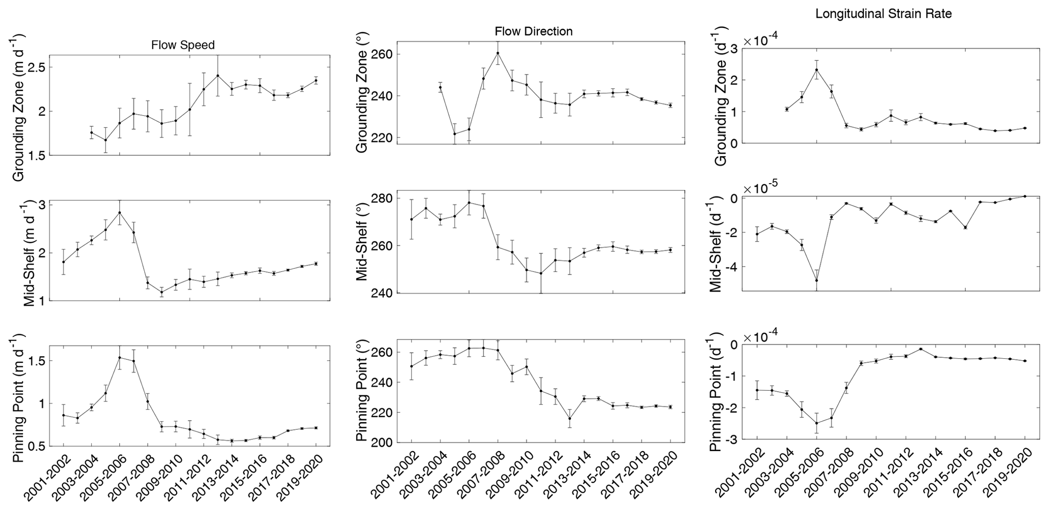
Figure 2Average values of speed, flow direction, and longitudinal strain rate at the three sites of interest (locations shown in Fig. 1) for the 20-year velocity record.
Figure 2 shows average values of ice-flow speed, direction, and longitudinal strain rate at the three sites. The change in ice speed over time yields the most consistent patterns in these different areas of the shelf, with all three showing a peak in speed between 2005 and 2007. Following this peak, the mid-shelf site displays a small but steady increase in speed to the end of the record, while the pinning point site experiences more variability, with an increase in speed only in the last 4 years of the record. The grounding zone site shows a large increase in speed following a brief deceleration around 2008, likely reflecting the transition from grounded to floating ice, when basal friction is released.
Flow directions are presented in grid directions based on the WGS84 Antarctic Polar Stereographic projection (EPSG:3031) used in all figures in this study. Grid north is 0∘, with values increasing clockwise. Following variability early in the record, flow directions at the grounding zone site are relatively stable. The mid-shelf and pinning point sites are stable early in the record, but both sites show an overall decrease in angle over time, with most of the decrease concentrated in the middle of the record, coincident with the large speed decrease seen in these boxes. This means that flow directions at these two sites shifted from grid west (270∘) or just south of grid west to a direction closer to grid south (counterclockwise) over time.
Longitudinal strain rates show greater contrast between the shelf areas. The peak in 2005–2006 at the grounding zone site is coincident in time with the speed increase noted in all three boxes. Patterns of longitudinal strain rate show the opposite trend at this time for the mid-shelf and pinning point sites, when both sites experience anomalously negative (compressional) strain rates. Following these anomalies, longitudinal strain rates in these boxes are approximately stable but with a slight increasing trend at the mid-shelf site. Longitudinal strain rates at that site switch from negative (compressional) to positive (extensional) in the last 2 years of the record, although the difference is very small.
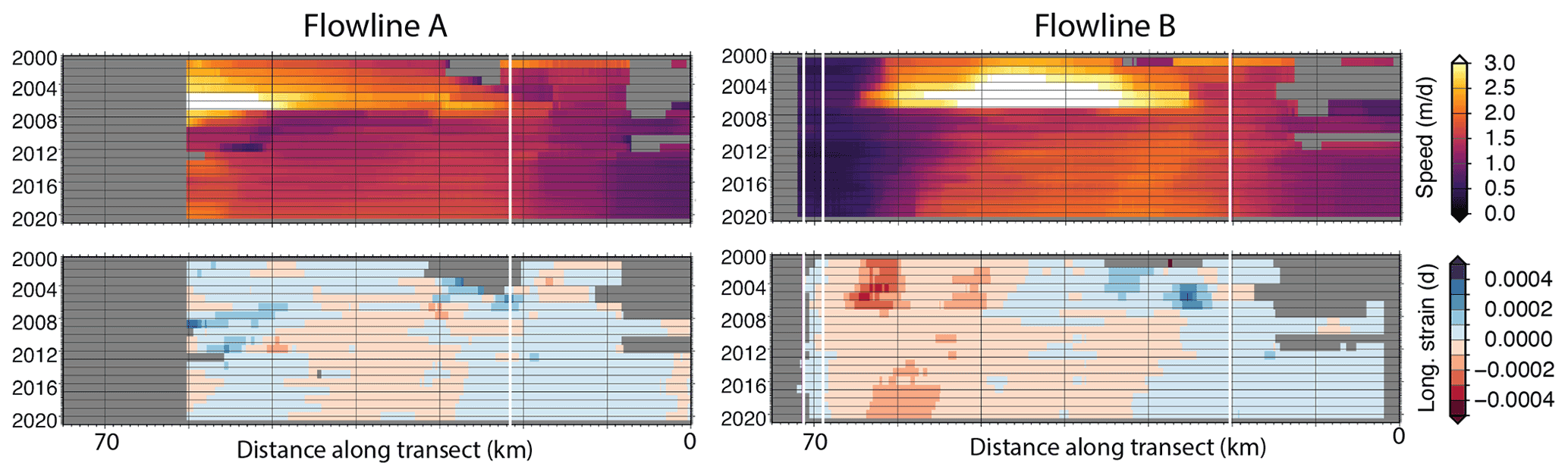
Figure 3Hovmöller diagrams of speed and longitudinal strain rates from our long-term record along Flowlines A and B (Fig. 1). Vertical white lines represent the location of the MEaSUREs 2011 grounding line (Rignot et al., 2016).
To provide some spatial context for the observed patterns in these areas of interest while easily visualizing change throughout the full record, we utilized Hovmöller diagrams along two flowlines of interest (grey solid lines in Fig. 1). These flowlines were generated based on Sentinel-1 data averaged between 2014 and 2020. Flowline A starts above the grounding line and flows through the main calving face of the TEIS towards grid north, while Flowline B starts above the grounding line and crosses the pinning point that confines the TEIS. The MEaSUREs 2011 grounding line (Rignot et al., 2016) is marked using vertical white lines on the Hovmöller diagrams in Fig. 3.
The speed records in Fig. 3 also show the increase in ice speed from the beginning of the record until ∼ 2007 as noted in the sites of interest examined in Fig. 2. This acceleration stretches from the grounding zone all the way to the calving front along Flowline A. The area of increased speed was confined to the region between the grounding zone and the pinning point on Flowline B, but it migrated towards the pinning point over time before the floating ice shelf decelerated drastically in 2007. Both flowlines show fairly small but uniform increases in velocity following the slowdown in 2007, a trend that is consistent along the full length of the flowlines. Similar to the more drastic increase in velocity between 2000 and 2007, this acceleration during the second half of the record migrates towards the pinning point along Flowline B.
Longitudinal strain rates are represented as positive in extension (blue) and negative in compression (red). Strain rates just downstream of the grounding zone and into the middle of the shelf were most extensive during the 2000–2007 acceleration. Extensional strain rates are also found near the calving front along Flowline A throughout the record. Otherwise, longitudinal strain rates are primarily compressional on the TEIS, particularly in the shear zone in front of the seaward pinning point. During the latter part of the record, the zone of compressional strain rates in the pinning point shear zone narrows and migrates towards the pinning point.
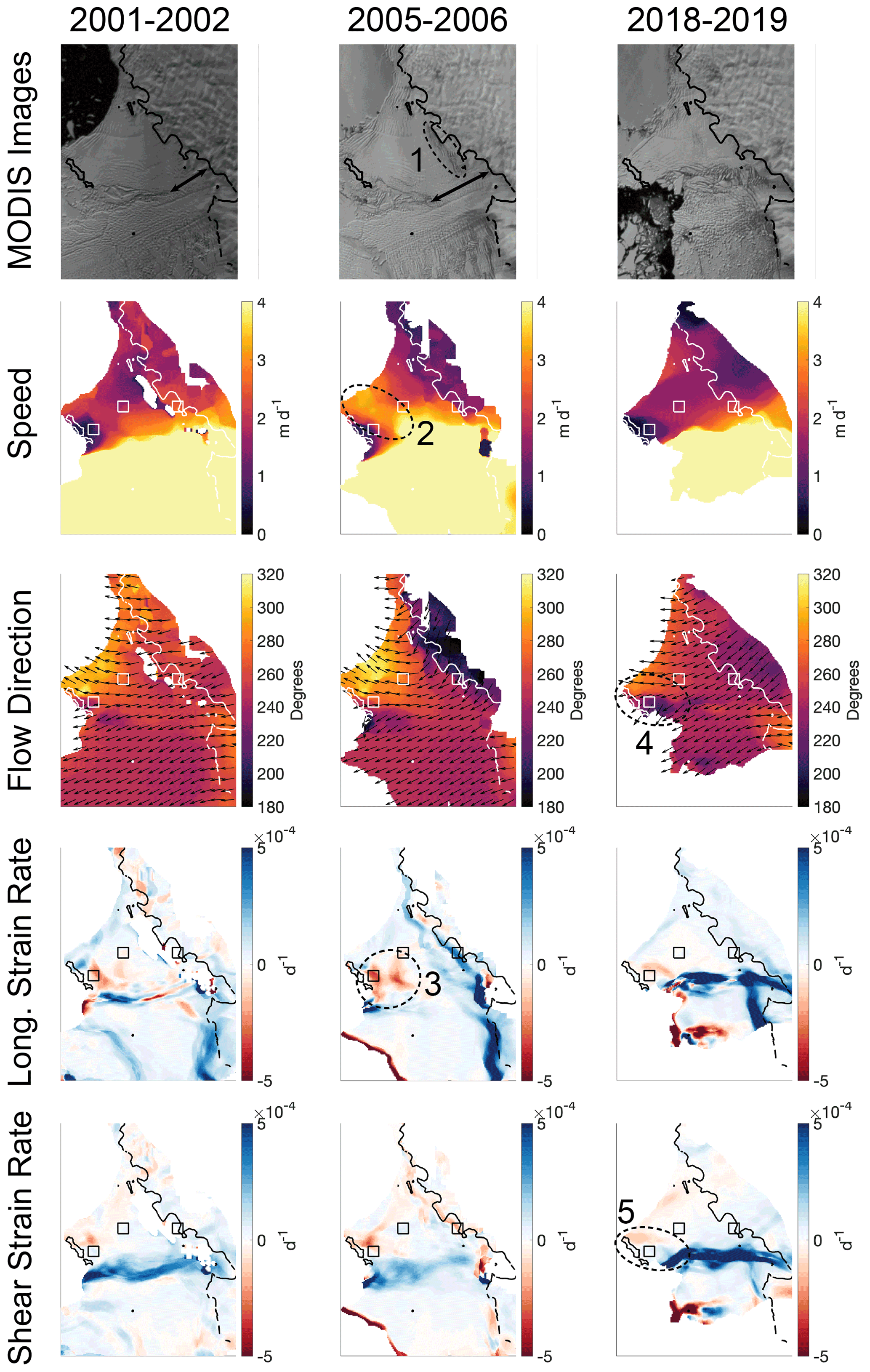
Figure 4Annual maps of TEIS variables. Arrows in the first two MODIS images indicate the length of the shear margin connecting the TEIS and TWIT early in the record. Dashed ovals 1, 2, and 3 highlight the crevasse swarm downstream of the grounding line, mid-shelf speed increase, and mid-shelf compressive strain rates, respectively, that all occurred around 2005–2006. Dashed ovals 4 and 5 highlight the flow direction split around the pining point and the resulting regions of contrasting sense of shear strain that are observed late in the record.
Patterns of change are captured in yet more spatial detail by examining maps of each variable. Videos that show maps of speed, flow direction, and strain-rate components (longitudinal, transverse, and shear) alongside MODIS imagery representative of each season are available at the US Antarctic Program Data Center (Alley et al., 2021). We highlight key frames from these videos in Fig. 4, including panels from early in the record (2001–2002), during the large acceleration event (2005–2006), and late in the record (2018–2019). These spatial patterns, along with the change in our site examples and the Hovmöller diagrams, are discussed in Sect. 4.
3.2 Five-year velocity and strain-rate record
In addition to the 20-year velocity record, we also produced a shorter-term, higher-temporal-resolution velocity record from 2015–2020, which we will refer to as our 5-year combined record. For each variable, we produced four averages per year: spring (September, October, November), summer (December, January, February), fall (March, April, May), and winter (June, July, August). The winter averages are primarily derived from Sentinel-1 radar data, as visible-band images are not available during polar winter, while the summer images combine both Sentinel-1 and visible-band images from Landsat-8 and MODIS.
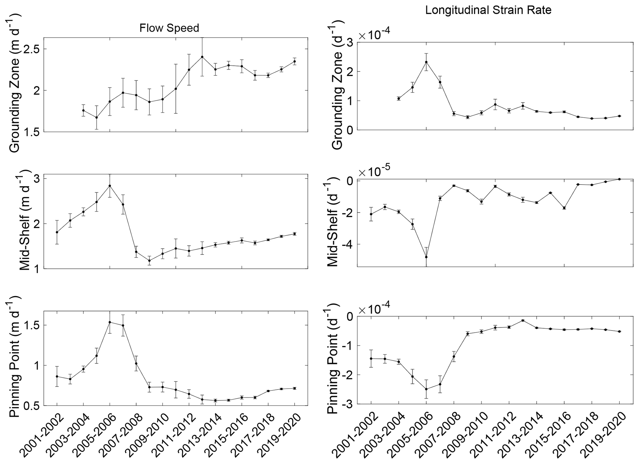
Figure 5Average values of speed, flow direction, and longitudinal strain rate at the three sites of interest (locations shown in Fig. 1) for the 5-year velocity record.
Figure 5 shows speed and longitudinal strain rates from the 5-year combined record averaged within the same study sites identified in Fig. 1. The trends in Fig. 5 are consistent with the long-term record trends shown in Fig. 2 at least in the last 3 years of the record, with increases in speed in all three boxes and more variability in the longitudinal strain rates. Notably, TEIS ice dynamics at these sites show no seasonal cycle that is detectable within the limits of our data and methodology. Variability may be due to external factors such as fast-ice presence that are outside the scope of this study.

Figure 6Hovmöller diagrams of speed and longitudinal strain rates from our 5-year combined record and from Sentinel-1 radar speckle tracking for Flowlines A and B (Fig. 1).
Considerably more detail can be seen in Hovmöller diagrams in Fig. 6, which display data from the same flowlines used in Fig. 3. Figure 6 provides data from our 5-year combined record, as well as from a monthly record based only on Sentinel-1 data. This Sentinel-1 record is at both a higher spatial (100 m) and temporal (monthly) resolution than our combined 5-year record. In addition, strain rates are calculated on a shorter (200 m) length scale rather than on the longer, approximately viscous (5 km) length scale used in our combined record. The Sentinel-1 data are therefore more appropriate for looking at details of change over small spatial length scales, such as in the shear zone upstream of the TEIS pinning point, as they preserve sharp gradients in dynamic properties. However, they are noisier because of the higher spatial resolution and because fewer images are available for averaging than in our 5-year combined record.
The migration of higher speeds towards the pinning point seen in the 20-year record is particularly evident in the Sentinel-1 record. Furthermore, the strongly negative longitudinal strain rates in this shear zone, which appear constant across it in the combined 5-year record, are seen to be concentrated in three distinct bands in the Sentinel-1 record, which we have marked with three black arrows in the bottom-right panel in Fig. 6. Two of these bands converge at the end of the record.
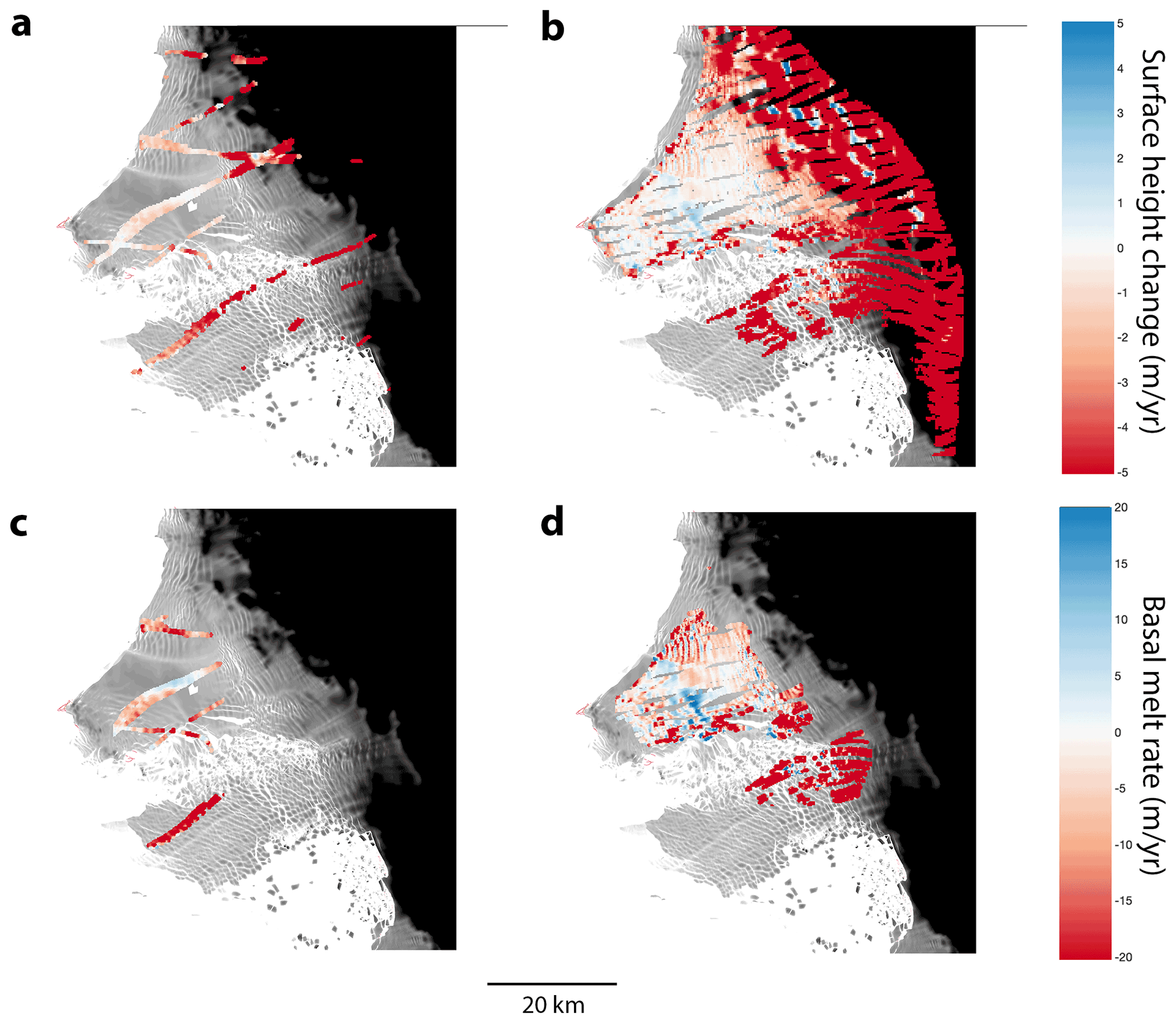
Figure 7Lagrangian surface lowering and basal melt rates. The first row shows surface lowering between ICESat and REMA (a) and between REMA and ICESat-2 (b). The second row shows basal melt rates between ICESat and REMA (c) and between REMA and ICESat-2 (d). Surface-height change and basal melt rates are interpolated to a standard 500 m grid using inverse distance weighting.
3.3 Surface elevation change and basal melt rates
Figure 7 shows surface-height change and basal melt rates calculated based on mass conservation on the TEIS. The left-hand column (Fig. 7a and c) shows change between ICESat (data points collected between 2003–2009) and REMA (DEM strips collected between 2013–2014), and the right-hand column (Fig. 7b and d) shows change between REMA and ICESat-2 (data points collected between 2018–2020). The first row (Fig. 7a and b) gives Lagrangian surface-height change, while the second row (Fig. 7c and d) gives calculated basal melt rates for pixels on the freely floating ice shelf. All points are plotted with ICESat or ICESat-2 points migrated to their locations when the REMA data were collected. Surface-height change and basal melt are calculated as annual averages over the time periods represented by each set of data points, and points are interpolated to a 500 m grid using inverse distance weighting.
The largest rates of surface-height change are found on grounded ice, both due to rapid dynamic thinning in these areas and because surface elevation changes on grounded ice are not hydrostatically compensated. Surface-height change on the floating ice shelf is overall much slower. We note an area in the middle of the TEIS that shows relatively rapid surface lowering in Fig. 7a, in the same location as relatively rapid surface-height increase in Fig. 7b. These same areas display rapid melt in Fig. 7c and rapid freeze in Fig. 7d. This small, anomalous region coincides with a seam between REMA DEM strips, with considerable feathering apparent in the mosaicking. While this may represent a real signal, the opposite signs of the signal in the two time periods suggest that the high rates of change here could also be due to REMA showing incorrectly low surface heights in this area.
Basal melt rates, which were calculated taking into account surface mass balance and vertical strain, generally reflect the same patterns as surface-height changes, suggesting that basal melt is the primary cause of surface-height changes on the floating TEIS. Variability in basal melt is particularly high in the shear zone upstream of the pinning point and in the heavily rifted area downstream of the grounding line in the grid-north quadrant. This variability may reflect inaccurate Lagrangian migration of points; areas with extensive rifting have widely varying ice thicknesses, which would clearly show inaccuracies in tracking of ice parcels. However, we also note that melt rates are typically much higher on near-vertical faces, and these vertical faces migrate laterally as a result, increasing basal melt rate variability in areas with highly variable ice thicknesses (e.g. Dutrieux et al., 2014).

Figure 8Landsat-7 and Landsat-8 time series of the TEIS from 2001–2020. Dashed ovals show the advection of a swarm of crevasses that opened downstream of the grounding line starting around 2005, and arrows show the formation of large rifts penetrating the centre of the TEIS starting around 2016. The rectangle in the 2020 images represents the subset area shown in Fig. 9.
4.1 Influence of the Thwaites Western Ice Tongue
The clearest dynamic control on the TEIS during the first half of the 20-year velocity record presented here is the Thwaites Western Ice Tongue (TWIT). The TWIT is the floating extension of the main trunk of Thwaites Glacier, and has speeds that are typically two to 4 times higher than those found on the TEIS. A prominent shear margin separates the TEIS and TWIT, which has had highly variable coherence throughout the record. Early in the record, a relatively short but strong shear margin was present near the grounding line, as indicated with a black arrow in the 2002 MODIS image in Fig. 4. The extent of this coherent, strong shear margin increased over the next several years, achieving its greatest length around 2006, as shown in the 2006 MODIS image in Fig. 4.
We deduce that this shear margin was strong based on both the lack of large fractures at this time and on the acceleration of the TEIS, supporting the interpretations of other authors (Miles et al., 2020; Mouginot et al., 2014). As shown in Figs. 2–4, the TEIS experienced significant acceleration early in the record, peaking around 2005–2007. The 2001–2002 map of speed in Fig. 4 shows that the highest speeds on TEIS at this time were found near the shear margin. We interpret this to be a result of large shearing stresses and higher TWIT speeds that dragged this part of TEIS forwards. This effect became most pronounced during the 2005–2006 season, when the zone of high speeds spread through the middle of the ice shelf, as marked with dashed oval 2 in the 2005–2006 speed image in Fig. 4. By 2007, large rifts developed across the shear margin (see MODIS images in videos provided in Alley et al., 2021), and by the 2008–2009 season a full separation between the TEIS and TWIT had developed in the shear margin. As it was no longer being dragged forwards by the TWIT, the TEIS decelerated significantly at this point. The TWIT nearly completely detached and disintegrated in the following years.
Acceleration on the TEIS while the shear margin was strong also added a new set of surface features to the TEIS. A swarm of crevasses opened along the grounding line during this increase in velocity, shown within dashed oval 1 in the 2006 MODIS image in Fig. 4, with more forming at the grounding line over the next few years. These crevasses are also visible in the Landsat time series of the TEIS shown in Fig. 8, starting in the 2005 image where we have marked their formation area with a dotted oval. The crevasse swarm can be seen to advect into the main floating ice shelf throughout the rest of the images in Fig. 8; we have indicated this swarm with another dotted oval in the 2020 image.
4.2 The TEIS pinning point and pinning point shear zone
Aside from the influence of the TWIT, the pinning point that confines the TEIS has had the greatest impact on the shelf's spatial patterns of ice-flow speed, direction, and strain rates. This pinning point transmits backstress upstream, as evidenced by the zone of slow velocities consistently found just upstream of the pinning point. That backstress is particularly evident in the 2005–2006 longitudinal strain-rate image in Fig. 4, which shows a large zone of negative (compressional) longitudinal strain rates upstream of the pinning point, which is marked with dashed oval 3. As the TWIT dragged the TEIS forwards at this time, the pinning point provided widespread resistance to this dragging.
Although the backstress transmitted from the pinning point is an overall stabilizing force for the TEIS, the clearest signs of destabilization are now concentrated in this area. As shown in Fig. 2, average flow directions on the shelf have rotated towards grid south (counter-clockwise) during the latter part of the 20-year record. When the TWIT was intact, the presence of the coherent ice tongue largely prevented the ice of the TEIS from outflowing in that direction. With the TWIT removed, TEIS ice flow is now showing strong patterns of divergence around the pinning point, as seen in the 2018–2019 flow direction image in Fig. 4 (marked with dashed oval 4). This directional divide is also clearly identifiable in the shear strain values in the 2018–2019 panel in Fig. 4 (marked with dashed oval 5), which shows a zone of left-lateral shearing that has developed to the grid south of the pinning point and right-lateral shearing to grid north.
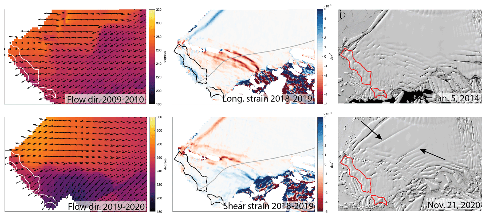
Figure 9Detail of the shear zone upstream of the TEIS pinning point showing the evolution of key features over time. First column: 2-year averages of flow direction, showing a split in flow direction around the pinning point that had not clearly developed by the 2009–2010 image, but had become very distinct by 2019–2020 image. Second column: longitudinal and shear strain rates derived from Sentinel-1 imagery showing distinct bands of high strain rates in the pinning point shear zone. Grey line is Flowline B (Fig. 1). Third column: Landsat-8 images showing the development of large rifts and smaller fractures nucleating in the pinning point shear zone. Red outline in all panels is the grounded pinning point from the 2011 MEaSUREs dataset (Rignot et al., 2016). Subset region is indicated in Fig. 8.
Figure 9 provides a close-up of the TEIS pinning point shear zone. The first column shows the 2009–2010 flow direction field, before the flow divergence was distinct, and the 2019–2020 flow direction field, which shows that the pattern has developed into distinct regions of contrasting flow direction with a boundary that closely coincides with the pinning point shear zone. The second column shows longitudinal and shear strain rates derived from Sentinel-1 data during summer 2018–2019. The top panel in this column shows the distinct bands of concentrated longitudinal strain rates noted in the Hovmöller diagram in Fig. 6. These bands of concentrated strain likely stretch farther towards the main calving front to grid northwest, but that region is subject to consistent data gaps during the record. Because the strain appears to be concentrating along rifts, shown in the Landsat-8 images in the third column of Fig. 9, which extend across most of the shelf in the shear zone, it is reasonable to assume that these concentrated bands of strain also extend across most of the shelf. The 2018–2019 Sentinel-1 shear strain rates in Fig. 9 show strain concentration in the same bands but reveal a contrasting sense of shear consistent with the split flow directions.
The Hovmöller diagrams in Fig. 6 show that the bands of concentrated strain rates migrate towards the pinning point over time, as does the region of higher speeds upstream of the pinning point shear zone. This migration is occurring at approximately the same speed as ice flow, which may indicate that these dynamic changes are advecting with the ice as the TEIS continues to adjust to the loss of the TWIT. However, the migration of concentrated strain and higher velocities towards the pinning point may alternatively or additionally indicate that the TEIS pinning point is ungrounding, removing backstress that has prevented this change in the past. The new flow divergence around the pinning point suggests that thinner ice is being delivered to the pinning point, which could promote ungrounding. Analysis of pinning point evolution is ongoing and will be presented in a separate paper.
Simultaneous with the development of divergence in ice flow around the pinning point, new, relatively small rifts have begun to form within the shear zone, and large, laterally extensive rifts have nucleated from the shear zone and extended into the middle of the shelf. These large rifts first appear in 2016 and are marked in the 2016 Landsat-8 image in Fig. 8, as well as in the 2020 Landsat-8 image in Fig. 9. As these rifts have formed within regions of high shear strain in the pinning point shear zone, they are likely caused at least in part by the new pattern of flow divergence around the pinning point.
In addition, Fig. 7 shows sustained, concentrated areas of relatively high rates of surface lowering and basal melt in the pinning point shear zone. Surface lowering and basal melt rates in this region are highly spatially variable, which may be related to variability in ice thickness and basal slope due to the presence of rifts and basal crevasses. Large differences in ice thickness may exaggerate errors in the Lagrangian migration of points, resulting in false variability in surface-height change and basal melt. However, there is also reason to believe that basal melt rates should be highly variable in fractured basal ice, as cold meltwater insulates relatively horizontal ice from melt while melt rates can be much higher on ice faces that are closer to vertical (e.g. Dutrieux et al., 2014). These values may therefore reflect localized high rates of real basal melt and thinning in this shear zone, which may also have contributed to the formation of large rifts within the shear zone.
4.3 TEIS and ocean forcing
Figure 7 shows that patterns of surface elevation change and patterns of basal melt on the floating ice shelf are very similar. Basal melt was calculated from mass conservation, taking into account surface mass balance and ice divergence (thinning/thickening due to horizontal strain) to explain the observed changes in surface height. Similarity between the patterns of basal melt and surface lowering suggests that surface mass balance and ice divergence contribute little to surface-height changes and that the vertical TEIS changes are driven by ocean forcing.
This is not an especially surprising result, as many studies (e.g. Pritchard et al., 2012) have shown that dynamic changes in the Amundsen Sea are driven by strong basal melt forcing by warm Circumpolar Deep Water (CDW). However, although CDW presence leads to an overall increase in ice-shelf basal melt and thinning, spatial and temporal details may be much more complex. Seroussi et al. (2017) ran a 50-year simulation of basal melt beneath the TEIS, showing that melt rates initially decrease as the ice-shelf base thins out of the reach of CDW, before melt rates increase with continued climate forcing. This separation from CDW on the relatively flat basal topography in the mid-TEIS may be responsible for the relatively low basal melt and thinning rates in this area, and it might even cause the mid-shelf area of freeze indicated by the calculated basal melt results. Although the ice draft is not significantly different than the middle of the shelf, the higher basal melt and thinning rates seen near the grounding line and pinning point shear zone may be due to the presence of steep basal topography prone to faster melt.
Another potential control on thinning in these areas may be directly related to patterns of ocean currents beneath the TEIS. Wåhlin et al. (2021) used CTD (conductivity, temperature, and depth) casts and an autonomous underwater vehicle to measure water properties near and beneath the TEIS during a 2019 cruise. Identified pathways of warm water inflow include previously underestimated branches from the east, roughly following bathymetric troughs beneath the main calving front of the TEIS and significant heat inflow through troughs from the north along the TWIT/TEIS shear margin. These observational data add considerable detail and new information to results produced by Nakayama et al. (2019), who used a high-resolution ocean model to show that increased basal melt rates on the TEIS coincide with faster sub-ice-shelf currents. Modelled (Nakayama et al., 2019) and observed (Wåhlin et al., 2021) warm inflows coincide roughly with the areas where we observe relatively large rates of thinning and bottom melting (Fig. 7), including near the grounding line to the east and in the shear zone upstream of the TEIS pinning point.
These results suggest that direct ocean forcing is a possible explanation for the earlier unpinning and disintegration of the TWIT. Modelled currents and melt rates were found to be faster beneath the TWIT than the TEIS (Nakayama et al., 2019), and the heat transport in one of the deep troughs leading under the TWIT/TEIS shear margin was very high (Wåhlin et al., 2021). Furthermore, Wåhlin et al. (2021) suggest that the ocean heat transport observed to be currently influencing the TEIS pinning point is unsustainably high and may lead to unpinning and destabilization in the style of the TWIT. Assuming that the TEIS pinning point experienced stable melt rates in previous decades, the observed high heat fluxes may be due to an externally forced change in ocean circulation, and/or could relate to a positive feedback where a reduction in ice-shelf draft due to basal melt allows for increased inflow of warm water. So, while the observed TEIS ice flow changes may be responding to ice-dynamic controls from the TWIT and upstream ice, they may also be directly due to ocean circulation changes that have increased heat fluxes and basal melt, thinning and weakening the ice shelf near the crucial TEIS pinning point.
The past 20 years of change on the TEIS were dominated by dynamic interaction with the neighbouring TWIT. Early in the record (∼ 2000–2006), the TEIS experienced large lateral stresses from the more rapidly flowing TWIT, causing the TEIS to accelerate. This was followed by rapid TEIS deceleration as the TWIT/TEIS shear margin weakened and the TWIT decoupled and disintegrated around 2007. The TEIS then developed new, independent flow patterns, including an overall ice velocity increase. The pinning point responsible for maintaining TEIS stability has now become an epicentre of destabilization. During the last several years of the record, ice flow has strongly diverged around the pinning point and strain rates have concentrated in narrow bands in the shear zone upstream. Simultaneously, significant fracturing has nucleated within the region of high strain rates and several rifts have penetrated much of the TEIS's central region.
Sparse measurements of surface lowering rates are available between ∼ 2003 and 2014 from ICESat and REMA, with much more detail available between ∼ 2014 and 2020 from REMA and ICESat-2. These data show generally low thinning and basal melt rates in the central TEIS, with much more variable and overall higher basal melt rates near the grounding line and in the shear zone upstream of the pinning point. The presence of relatively high thinning rates is particularly important in the pinning point shear zone, where basal melt may be partially responsible for weakening that has led to new rift formation.
Both the vertical and horizontal changes observed on the TEIS over the last 20 years indicate progressive weakening and destabilization of the floating ice shelf. There is no indication that these trends will reverse in the future. Increased forcing by CDW is likely to continue (e.g. Holland et al., 2019), and upstream acceleration and thinning of Thwaites Glacier means that ice advected onto the shelf may be more damaged (e.g. MacGregor et al., 2012). The patterns of dynamic instability that we have observed indicate that weakening will enhance over time (see also Joughin et al., 2014; Rignot et al., 2014). Based on this analysis, the future of the TEIS looks much like what we have already seen on the TWIT: a total or near-total loss of the floating ice shelf, removing the buttressing connection with the pinning point and resulting in acceleration of grounded ice. We suggest that final disintegration of the TEIS will occur in one of three possible ways:
The surface crevasse swarm that nucleated at the grounding zone around 2005 will continue to advect, reaching the central region of the shelf that is now penetrated by large rifts. These damaged areas will join in 10–20 years and may destabilize the TEIS throughout its central region. The impact of this event will depend on whether new, large rifts continue to nucleate from the pinning point shear zone, and the evolution of the crevasse swarm (further extension or healing) as it continues to advect. The condition of the crevasse swarm will depend largely on mid-shelf longitudinal strain rates, which are primarily compressional but are trending towards neutral or extensional.
The ice shelf may decouple from the pinning point due to large-scale failure in the pinning point shear zone. Based on the rapid development of rifting within the shear zone in the last ∼ 5 years, this could plausibly occur on a timescale of years to decades. The pace of this failure is likely to be set by the basal melt rate and the continued concentration of stress along large rifts extending across the pinning point shear zone. We note, however, that break-up of other ice shelves has been highly non-linear and that a sufficiently thin and weak shelf can break up very rapidly.
Continued ocean-forced thinning of the ice shelf and advection of thinner ice onto the pinning point will result in partial or complete unpinning of the ice shelf and loss of integrity. The extensive flow changes and migration of high velocities towards the pinning point over the last decade suggest that this process is underway and could destabilize the shelf in 1 to 2 decades.
To estimate the error in our calculations of basal melt rates, we use standard equations of error propagation. First, we find the error associated with ice thickness. We rearrange Eq. (2) from the main text to solve for H and then propagate the error:
Error in first term (Zs) on the top of the fraction is σ1REMA = 6 m for the REMA mosaic and σ1ICES = 0.2 m for ICESat and ICESat-2. Error in ha is = 1 m, which takes into account the time variability in firn-air content as described in the text. The error in the second term can then be expressed as follows:
We use error propagation for addition and subtraction for the top of the fraction in Eq. (A1):
where σH_top = 6.1 m for REMA and 0.91 m for ICESat/ICESat-2. Then we divide by the constant value on the bottom in Eq. (A1) to get the total error in H for REMA and for ICESat/ICESat-2: σH_REMA = 57 m and σH_ICES = 8.6 m.
Now we find the error in basal melt rate by propagating the error in ice thickness and other terms through Eq. (3) from the main text (repeated here for reference):
To find the error in the first term, we start with error propagation for addition and subtraction, then divide by Dt:
This yields an error estimate of σDHDT = 11.5 m yr−1 for REMA to ICESat-2 and σDHDT = 7.2 m yr−1 for ICESat to REMA. Error in second term is treated as a constant multiplied by added uncorrelated errors:
Error in is estimated to be 0.1 m of ice equivalent per year. Altogether, therefore, the error in basal melt rate is calculated as
This yields an error estimate of = 11.5 m yr−1 for REMA to ICESat-2 and = 7.2 m yr−1 for ICESat to REMA.
Data sources are cited in the text. Derived velocity and strain-rate records are available through the US Antarctic Program Data Center (Alley et al., 2021, https://doi.org/10.15784/601478).
KEA led data analysis and writing. CTW produced alpha maps and assisted in analysis of altimetry and REMA data. AL analysed all Sentinel-1 data and provided figures for the article. CTW, TAS, MT, ECP, and AM assisted in data analysis and article planning. BW and MK provided data and expertise in MODIS imagery and PyCorr processing. TS and CH assisted in processing of ICESat-2 data. SFC assisted in analysis of the REMA DEM in relation to ICESat and ICESat-2 data. JTML, MM, EK, and DD provided data processing for firn-air thickness and surface mass balance used in basal melt rate calculations. All authors participated in the writing and revision of the article.
The authors declare that they have no conflict of interest.
Publisher's note: Copernicus Publications remains neutral with regard to jurisdictional claims in published maps and institutional affiliations.
This work is from the TARSAN project, a component of the International Thwaites Glacier Collaboration (ITGC). Logistics were provided by NSF, U.S. Antarctic Program, and NERC, British Antarctic Survey. Sentinel-1 data were provided by the Copernicus Program of the European Commission. We thank Fernando Paolo, Luc Girod, and Richard Alley for advice on data preparation methods, as well as Anna Wåhlin for her comments on this article.
This research has been supported by the National Science Foundation, Directorate for Geosciences (grant no. 1929991), and the Natural Environment Research Council, British Antarctic Survey (grant no. NE/S006419/1).
This paper was edited by Nicolas Jourdain and reviewed by three anonymous referees.
Alley, K. E., Scambos, T. A., Anderson, R. S., Rajaram, H., Pope, A., and Haran, T. M.: Continent-wide estimates of Antarctic strain rates from Landsat 8-derived velocity grids, J. Glaciol., 64, 321–332, https://doi.org/10.1017/jog.2018.23, 2018.
Alley, K. E., Wild, C. T., Scambos, T. A., Muto, A., Pettit, E.,Truffer, M., Wallin, B., and Klinger, M.: Two-year velocity and strain-rate averages from the Thwaites Eastern Ice Shelf, 2001–2020 U.S. Antarctic Program (USAP) Data Center [data set], https://doi.org/10.15784/601478, 2021.
Bell, B., Hersbach, H., Berrisford, P., Dahlgren, P., Horányi, A., Sabater, J. M., Nicolas, J., Radu, R., Schepers, D., Simmons, A., Soci, C., and Thépaut, J.-N.: ERA5 hourly data on single levels from 1950 to 1978 (preliminary version), Copernicus Climate Change Service (C3S) Climate Data Store (CDS), available at: https://cds.climate.copernicus.eu/cdsapp#!/dataset/reanalysis-era5-single-levels?tab=overview (last access: 9 November 2021), 2020.
Bindschadler, R., Choi, H., Wichlacz, A., Bingham, R., Bohlander, J., Brunt, K., Corr, H., Drews, R., Fricker, H., Hall, M., Hindmarsh, R., Kohler, J., Padman, L., Rack, W., Rotschky, G., Urbini, S., Vornberger, P., and Young, N.: Getting around Antarctic: new high-resolution mappings of the grounded and freely-floating boundaries of the Antarctic ice sheet created for the International Polar Year, The Cryosphere, 5, 569–588, https://doi.org/10.5194/tc-5-569-2011, 2011.
Borsa, A. A., Moholdt, G., Fricker, H. A., and Brunt, K. M.: A range correction for ICESat and its potential impact on ice-sheet mass balance studies, The Cryosphere, 8, 345–357, https://doi.org/10.5194/tc-8-345-2014, 2014.
Brunt, K. M., Neumann, T. A., and Smith, B. E.: Assessment of ICESat-2 Ice Sheet Surface Heights, Based on Comparisons Over the Interior of the Antarctic Ice Sheet, Geophys. Res. Lett., 46, 13072–13078, https://doi.org/10.1029/2019gl084886, 2019.
Chen, J., Ke, C., Zhou, X., Shao, Z., and Li, L.: Surface velocity estimations of ice shelves in the northern Antarctic Peninsula derived from MODIS data, J. Geogr. Sci., 26, 243–256, 2016.
Dorandeu, J. and Traon, P. Y. L.: Effects of Global Mean Atmospheric Pressure Variations on Mean Sea Level Changes from TOPEX/Poseidon, J. Atmos. Ocean. Tech., 16, 1279–1283, https://doi.org/10.1175/1520-0426(1999)016<1279:EOGMAP>2.0.CO;2, 1999.
Dupont, T. K. and Alley, R. B.: Assessment of the importance of ice-shelf buttressing to ice-sheet flow, Geophys. Res. Lett., 32, L04503, https://doi.org/10.1029/2004gl022024, 2005.
Dutrieux, P., Stewart, C., Jenkins, A., Nicholls, K. W., Corr, H. F. J., Rignot, E., and Steffen, K.: Basal terraces on melting ice shelves, Geophys. Res. Lett., 41, 5506–5513, https://doi.org/10.1002/2014gl060618, 2014.
Egbert, G. D. and Erofeeva, S. Y.: Efficient Inverse Modeling of Barotropic Ocean Tides, J. Atmos. Ocean. Tech., 19, 183–204, https://doi.org/10.1175/1520-0426(2002)019<0183:eimobo>2.0.co;2, 2002.
Fahnestock, M., Scambos, T., Moon, T., Gardner, A., Haran, T., and Klinger, M.: Rapid large-area mapping of ice flow using Landsat 8, Remote Sens. Environ., 185, 84–94, https://doi.org/10.1016/j.rse.2015.11.023, 2016.
Fürst, J. J., Durand, G., Gilet-Chaulet, F., Tavard, L., Rankl, M., Braun, M., and Gagliardini, O.: The safety band of Antarctic ice shelves, Nature, 6, 479–482, https://doi.org/10.1038/NCLIMATE2912, 2016.
Gardner, A. S., Fahnestock, M. A., and Scambos, T. A.: ITS_LIVE Regional Glacier and Ice Sheet Surface Velocities, National Snow and Ice Data Center [data set], CO, https://doi.org/10.5067/6II6VW8LLWJ7, 2019.
Gelaro, R., McCarty, W., Suárez, M. J., Todling, R., Molod, A., Takacs, L., Randles, C. A., Darmenov, A., Bosilovich, M. G., Reichle, R., Wargan, K., Coy, L., Cullather, R., Draper, C., Akella, S., Buchard, V., Conaty, A., da Silva, A. M., Gu, W., Kim, G.-K., Koster, R., Lucchesi, R., Merkova, D., Nielsen, J. E., Partyka, G., Pawson, S., Putman, W., Rienecker, M., Schubert, S. D., Sienkiewicz, M., and Zhao, B.: The Modern-Era Retrospective Analysis for Research Applications, Version 2 (MERRA-2), J. Climate, 30, 5419–5454, https://doi.org/10.1175/JCLI-D-16-0758.1, 2017.
Greene, C. A., Gwyther, D. E., and Blankenship, D. D.: Antarctic Mapping Tools for Matlab, Comput. Geosci., 104, 151–157, https://doi.org/10.1016/j.cageo.2016.08.003, 2017.
Greene, C. A., Young, D. A., Gwyther, D. E., Galton-Fenzi, B. K., and Blankenship, D. D.: Seasonal dynamics of Totten Ice Shelf controlled by sea ice buttressing, The Cryosphere, 12, 2869–2882, https://doi.org/10.5194/tc-12-2869-2018, 2018.
Han, H. and Lee, H.: Tide deflection of Campbell Glacier Tongue, Antarctica, analyzed by double-differential SAR interferometry and finite element method, Remote Sens. Environ., 141, 201–213, https://doi.org/10.1016/j.rse.2013.11.002, 2014.
Haug, T., Kääb, A., and Skvarca, P.: Monitoring ice shelf velocities from repeat MODIS and Landsat data – a method study on the Larsen C ice shelf, Antarctic Peninsula, and 10 other ice shelves around Antarctica, The Cryosphere, 4, 161–178, https://doi.org/10.5194/tc-4-161-2010, 2010.
Holland, P. R., Bracegirdle, T. J., Dutrieux, P., Jenkins, A., and Steig, E. J.: West Antarctic ice loss influenced by internal climate variability and anthropogenic forcing, Nat. Geosci., 12, 718–724, https://doi.org/10.1038/s41561-019-0420-9, 2019.
Howat, I. M., Porter, C., Smith, B. E., Noh, M.-J., and Morin, P.: The Reference Elevation Model of Antarctica, The Cryosphere, 13, 665–674, https://doi.org/10.5194/tc-13-665-2019, 2019.
Hughes, T. J.: The weak underbelly of the West Antarctic ice sheet, J. Glaciol., 27, 518–525, https://doi.org/10.3189/s002214300001159x, 1981.
Jenkins, A. and Doake, C. S. M.: Ice-ocean interaction on Ronne Ice Shelf, Antarctica, J. Geophys. Res., 96, 791–813, https://doi.org/10.1029/90jc01952, 1991.
Joughin, I., Smith, B. E., and Medley, B.: Marine Ice Sheet Collapse Potentially Under Way for the Thwaites Glacier Basin, West Antarctica, Science, 344, 735–738, https://doi.org/10.1126/science.1249055, 2014.
Keenan, E., Wever, N., Dattler, M., Lenaerts, J. T. M., Medley, B., Kuipers Munneke, P., and Reijmer, C.: Physics-based SNOWPACK model improves representation of near-surface Antarctic snow and firn density, The Cryosphere, 15, 1065–1085, https://doi.org/10.5194/tc-15-1065-2021, 2021.
MacGregor, J. A., Catania, G. A., Markowski, M. S., and Andrews, A. G.: Widespread rifting and retreat of ice-shelf margins in the eastern Amundsen Sea Embayment between 1972 and 2011, J. Glaciol., 58, 458–466, https://doi.org/10.3189/2012jog11j262, 2012.
Mathers, E. L.: Vistas for Geodesy in the New Millennium, IAG 2001 Scientific Assembly, Budapest, Hungary, 2–7 September 2001, Iag Symp, 523–528, https://doi.org/10.1007/978-3-662-04709-5_88, 2002.
Mercer, J. H.: West Antarctic ice sheet and CO2 greenhouse effect: a threat of disaster, Nature, 271, 321–325, https://doi.org/10.1038/271321a0, 1978.
Miles, B. W. J., Stokes, C. R., Jenkins, A., Jordan, J. R., Jamieson, S. S. R., and Gudmundsson, G. H.: Intermittent structural weakening and acceleration of the Thwaites Glacier Tongue between 2000 and 2018, J. Glaciol., 66, 485–495, https://doi.org/10.1017/jog.2020.20, 2020.
Milillo, P., Rignot, E., Rizzoli, P., Scheuchl, B., Mouginot, J., Bueso-Bello, J., and Prats-Iraola, P.: Heterogeneous retreat and ice melt of Thwaites Glacier, West Antarctica, Science Advances, 5, eaau3433, https://doi.org/10.1126/sciadv.aau3433, 2019.
Morlighem, M.: MEaSUREs BedMachine Antarctica, Version 2, NASA National Snow and Ice Data Center Distributed Active Archive Center, Boulder [data set], CO, https://doi.org/10.5067/E1QL9HFQ7A8M, 2020.
Morlighem, M., Rignot, E., Binder, T., Blankenship, D., Drews, R., Eagles, G., Eisen, O., Ferraccioli, F., Forsberg, R., Fretwell, P., Goel, V., Greenbaum, J. S., Gudmundsson, H., Guo, J., Helm, V., Hofstede, C., Howat, I., Humbert, A., Jokat, W., Karlsson, N. B., Lee, W. S., Matsuoka, K., Millan, R., Mouginot, J., Paden, J., Pattyn, F., Roberts, J., Rosier, S., Ruppel, A., Seroussi, H., Smith, E. C., Steinhage, D., Sun, B., van den Broeke, M. R., van Ommen, T. D., van Wessem, M., and Young, D. A.: Deep glacial troughs and stabilizing ridges unveiled beneath the margins of the Antarctic ice sheet, Nat. Geosci., 13, 132–137, https://doi.org/10.1038/s41561-019-0510-8, 2020.
Mouginot, J., Rignot, E., and Scheuchl, B.: Sustained increase in ice discharge from the Amundsen Sea Embayment, West Antarctica, from 1973 to 2013, Geophys. Res. Lett., 41, 1576–1584, https://doi.org/10.1002/2013gl059069, 2014.
Mouginot, J., Scheuchl, B., and Rignot, E.: MEaSUREs Annual Antarctic Ice Velocity Maps 2005-2017, Version 1. 2005–2013, NASA National Snow and Ice Data Center Distributed Active Archive Center [data set], CO, https://doi.org/10.5067/9T4EPQXTJYW9, 2017.
Nakayama, Y., Manucharyan, G., Zhang, H., Dutrieux, P., Torres, H. S., Klein, P., Seroussi, H., Schodlok, M., Rignot, E., and Menemenlis, D.: Pathways of ocean heat towards Pine Island and Thwaites grounding lines, Sci. Rep.-UK, 9, 16649, https://doi.org/10.1038/s41598-019-53190-6, 2019.
Padman, L., Fricker, H. A., Coleman, R., Howard, S., and Erofeeva, L.: A new tide model for the Antarctic ice shelves and seas, Ann. Glaciol., 34, 247–254, https://doi.org/10.3189/172756402781817752, 2002.
Padman, L., Erofeeva, S. Y., and Fricker, H. A.: Improving Antarctic tide models by assimilation of ICESat laser altimetry over ice shelves, Geophys. Res. Lett., 35, https://doi.org/10.1029/2008gl035592, 2008.
Paolo, F. S., Fricker, H. A., and Padman, L.: Constructing improved decadal records of Antarctic ice shelf height change from multiple satellite radar altimeters, Remote Sens. Environ., 177, 192–205, https://doi.org/10.1016/j.rse.2016.01.026, 2016.
Pritchard, H. D., Ligtenberg, S. R. M., Fricker, H. A., Vaughan, D. G., van den Broeke, M. R., and Padman, L.: Antarctic ice-sheet loss driven by basal melting of ice shelves, Nature, 484, 502–505, https://doi.org/10.1038/nature10968, 2012.
Reese, R., Gudmundsson, G. H., Levermann, A., and Winkelmann, R.: The far reach of ice-shelf thinning in Antarctica, Nat. Clim. Change, 8, 53–57, https://doi.org/10.1038/s41558-017-0020-x, 2017.
Rignot, E.: Evidence for rapid retreat and mass loss of Thwaites Glacier, West Antarctica, J. Glaciol., 47, 213–222, https://doi.org/10.3189/172756501781832340, 2001.
Rignot, E., Mouginot, J., Morlighem, M., Seroussi, H., and Scheuchl, B.: Widespread, rapid grounding line retreat of Pine Island, Thwaites, Smith, and Kohler glaciers, West Antarctica, from 1992 to 2011, Geophys. Res. Lett., 41, 3502–3509, https://doi.org/10.1002/2014gl060140, 2014.
Rignot, E., Mouginot, J., and Scheuchl, B.: MEaSUREs Antarctic Grounding Line from Differential Satellite Radar Interferometry, Version 2, NASA National Snow and Ice Data Center Distributed Active Archive Center [data set], CO, https://doi.org/10.5067/IKBWW4RYHF1Q, 2016.
Scambos, T., Fahnestock, M., Gardner, A., and Klinger, M.: Global Land Ice Velocity Extraction from Landsat 8 (GoLIVE), Version 1, NSID: National Snow and Ice Data Center, CO, https://doi.org/10.7265/N5ZP442B, 2016.
Scambos, T. A., Bohlander, J., and Raup, B.: Images of Antarctic Ice Shelves, National Snow and Ice Data Center [data set], CO, https://doi.org/10.7265/N5NC5Z4N, 1996.
Scambos, T. A., Bell, R. E., Alley, R. B., Anandakrishnan, S., Bromwich, D. H., Brunt, K., Christianson, K., Creyts, T., Das, S. B., DeConto, R., Dutrieux, P., Fricker, H. A., Holland, D., MacGregor, J., Medley, B., Nicolas, J. P., Pollard, D., Siegfried, M. R., Smith, A. M., Steig, E. J., Trusel, L. D., Vaughan, D. G., and Yager, P. L.: How much, how fast? A science review and outlook for research on the instability of Antarctica's Thwaites Glacier in the 21st century, Glob. Planet. Change, 153, 16–34, https://doi.org/10.1016/j.gloplacha.2017.04.008, 2017.
Seroussi, H., Nakayama, Y., Larour, E., Menemenlis, D., Morlighem, M., Rignot, E., and Khazendar, A.: Continued retreat of Thwaites Glacier, West Antarctica, controlled by bed topography and ocean circulation, Geophys. Res. Lett., 44, 6191–6199, https://doi.org/10.1002/2017gl072910, 2017.
Smith, B., Fricker, H. A., Gardner, A., Siegfried, M. R., Adusumilli, S., Csathó, B. M., Holschuh, N., Nilsson, J., Paolo, F. S., and the ICESat-2 Science Team: ATLAS/ICESat-2 L3A Land Ice Height, version 1, National Snow and Ice Data Center [data set], CO, https://doi.org/10.5067/atlas/atl06.001, 2019.
Smith, B., Fricker, H. A., Gardner, A. S., Medley, B., Nilsson, J., Paolo, F. S., Holschuh, N., Adusumilli, S., Brunt, K., Csatho, B., Harbeck, K., Markus, T., Neumann, T., Siegfried, M. R., and Zwally, H. J.: Pervasive ice sheet mass loss reflects competing ocean and atmosphere processes, Science, 368, 1239–1242, https://doi.org/10.1126/science.aaz5845, 2020.
Tinto, K. J. and Bell, R. E.: Progressive unpinning of Thwaites Glacier from newly identified offshore ridge: Constraints from aerogravity, Geophys. Res. Lett., 38, L20503, https://doi.org/10.1029/2011gl049026, 2011.
Wåhlin A. K., Graham, A., Hogan, K. A., Queste, B. Y., Boehme, L., Larter, R., Pettit, E., Wellner, J., and Heywood, K. J.: Pathways and modification of warm water flowing beneath Thwaites ice shelf, West Antarctica, Science Advances, 7, eabd7254, https://doi.org/10.1126/sciadv.abd7254, 2021.
Walker, R. T., Parizek, B. R., Alley, R. B., Anandakrishnan, S., Riverman, K. L., and Christianson, K.: Ice-shelf tidal flexure and subglacial pressure variations, Earth Planet. Sc. Lett., 361, 422–428, https://doi.org/10.1016/j.epsl.2012.11.008, 2013.
Weertman, J.: Stability of the Junction of an Ice Sheet and an Ice Shelf, J. Glaciol., 13, 3–11, https://doi.org/10.1017/s0022143000023327, 1974.
Wild, C. T., Marsh, O. J., and Rack, W.: Differential interferometric synthetic aperture radar for tide modelling in Antarctic ice-shelf grounding zones, The Cryosphere, 13, 3171–3191, https://doi.org/10.5194/tc-13-3171-2019, 2019.
Wolfe, R. E., Nishihama, M., Fleig, A. J., Kuyper, J. A., Roy, D. P., Storey, J. C., and Patt, F. S.: Achieving sub-pixel geolocation accuracy in support of MODIS land science, Remote Sens. Environ., 83, 31–49, https://doi.org/10.1016/s0034-4257(02)00085-8, 2002.
Zwally, H. J., Schutz, R., Bentley, C., Bufton, J., Herring, T., Minster, J., Spinhirne, J., and Thomas, R.: GLAS/ICESat L2 Antarctic and Greenland Ice Sheet Altimetry Data, version 34, National Snow and Ice Data Center [data set], CO, https://doi.org/10.5067/ICESAT/GLAS/DATA225, 2014.