the Creative Commons Attribution 4.0 License.
the Creative Commons Attribution 4.0 License.
 | 09 Nov 2021
The contribution of melt ponds to enhanced Arctic sea-ice melt during the Last Interglacial
Rachel Diamond
Louise C. Sime
David Schroeder
Maria-Vittoria Guarino
The Hadley Centre Global Environment Model version 3 (HadGEM3) is the first coupled climate model to simulate an ice-free Arctic during the Last Interglacial (LIG), 127 000 years ago. This simulation appears to yield accurate Arctic surface temperatures during the summer season. Here, we investigate the causes and impacts of this extreme simulated ice loss. We find that the summer ice melt was predominantly driven by thermodynamic processes: atmospheric and ocean circulation changes did not significantly contribute to the ice loss. We demonstrate these thermodynamic processes were significantly impacted by melt ponds, which formed on average 8 d earlier during the LIG than during the pre-industrial control (PI) simulation. This relatively small difference significantly changed the LIG surface energy balance and impacted the albedo feedback. Compared to the PI simulation: in mid-June, of the absorbed flux at the surface over ice-covered cells (sea-ice concentration > 0.15), ponds accounted for 45 %–50 %, open water 35 %–45 %, and bare ice and snow 5 %–10 %. We show that the simulated ice loss led to large Arctic sea surface salinity and temperature changes. The sea surface temperature and salinity signals we identify here provide a means to verify, in marine observations, if and when an ice-free Arctic occurred during the LIG. Strong LIG correlations between spring melt pond and summer ice area indicate that, as Arctic ice continues to thin in future, the spring melt pond area will likely become an increasingly reliable predictor of the September sea-ice area. Finally, we note that models with explicitly modelled melt ponds seem to simulate particularly low LIG sea-ice area. These results show that models with explicit (as opposed to parameterised) melt ponds can simulate very different sea-ice behaviour under forcings other than the present day. This is of concern for future projections of sea-ice loss.
- Article
(3368 KB) - Full-text XML
-
Supplement
(1282 KB) - BibTeX
- EndNote


Interglacials are periods of globally higher temperatures which occur between cold glacial periods (Sime et al., 2009; Otto-Bliesner et al., 2013; Fischer et al., 2018). Glacial–interglacial cycles are largely driven by changes in the Earth’s orbit which affect incoming radiation. The Eemian period, here called the Last Interglacial or LIG, occurred 130 000–116 000 years ago. At high latitudes orbital forcing led to summertime top-of-atmosphere short-wave (TOA SW) radiation 60–75 Wm−2 greater for the LIG, compared to the pre-industrial (PI) period (Kageyama et al., 2021; Guarino et al., 2020b). This drove differences between the LIG and PI surface energy balance. Whilst the significance of these PI to LIG surface energy balance differences vary between climate models (Lunt et al., 2013; Otto-Bliesner et al., 2013), proxy records of the LIG indicate that mean Arctic summer land temperature was +4–5 K higher than the PI (CAPE members, 2006).
Prior to 2020, most climate models simulated LIG temperatures which were too cool compared with LIG temperature data (Otto-Bliesner et al., 2013; IPCC, 2013). Recently, Guarino et al. (2020b) found that the loss of Arctic sea ice in the summer likely drove these warm Arctic temperatures. As discussed below, Guarino et al. (2020b) suggested that melt ponds may have been a significant driver of ice loss and that previous climate models, with a less comprehensive representation of melt ponds, may not have simulated the loss of enough Arctic sea ice during the LIG. Kageyama et al. (2021) explored the ocean-core-based proxy records of LIG Arctic sea-ice change. They found that sea-ice changes are more difficult to determine than temperature changes, with some conflicting interpretations of proxy data from the available records and imprecision in dating materials from cores in the high Arctic. This makes it difficult to determine the mechanisms or distribution of sea-ice loss during the LIG from these preserved biological data.
In terms of understanding mechanisms that drove Arctic sea-ice change during the LIG, three main factors are known to affect summer sea-ice behaviour: albedo feedbacks (Curry et al., 1995), cloud cover feedbacks (Kay and Gettelman, 2009), and ocean heat transport changes (Årthun et al., 2019; Auclair and Tremblay, 2018). As well as these, changes to sea-ice distribution caused by changes to wind patterns and ocean circulation may also affect summer sea-ice extent (Kageyama et al., 2021; Deser and Teng, 2008; Wang et al., 2009). Albedo feedbacks are strongly influenced by melt ponds, systems of pools that form from meltwater and begin to collect on the Arctic ice surface in spring. Pond-covered ice has a lower albedo, at 0.1–0.5, than bare ice, at 0.6–0.65, or snow, at 0.84–0.87 (Perovich et al., 2002b; Eicken et al., 2004; Perovich and Tucker, 1997). Pond-covered ice thus absorbs a higher fraction of incident solar radiation and transmits a greater fraction of incident radiation to the ice and ocean below. This difference accelerates the melting of the ice beneath ponds, with melt rates of pond-covered ice up to 2–3 times the melt rate of bare ice (Fetterer and Untersteiner, 1998). Over the last decades, melt ponds have played a key role in reducing the surface albedo (Eicken et al., 2004; Maslanik et al., 2007; Perovich et al., 2007); throughout melt season, nearly 60 % of the summer sea-ice area may be covered by ponds (Fetterer and Untersteiner, 1998; Eicken et al., 2004).
In spite of their importance, melt ponds have only rather recently been explicitly included in Coupled Model Intercomparison Project (CMIP) models. In CMIP6 models, the most common approach is to implicitly parameterise melt ponds by reducing the ice/snow albedo when surface ice temperatures approach 0 ∘C (e.g. Collins et al., 2006; Curry et al., 2001). This tuning has been relatively successful for reproducing realistic melt rates for the present day (Collins et al., 2006; Curry et al., 2001). However, pond formation is affected by sea-ice processes throughout melt season (e.g. evolving topography and snow cover), which this tuning does not represent (Kwok et al., 2009). Therefore, in recent years, there has been increasing interest in incorporating more detailed melt pond models into global climate models (GCMs). The Hadley Centre Global Environment Model version 3 (HadGEM3) includes one of the most comprehensive, to date, melt pond schemes in its sea-ice component CICE5.1 (Hunke et al., 2015, detailed in Sect. 2), a result of a series of developments and improvements (Taylor and Feltham, 2004; Lüthje et al., 2006; Skyllingstad et al., 2009; Scott and Feltham, 2010; Flocco et al., 2012).
The Coupled Model Intercomparison Project Phase 6 (CMIP6) Palaeoclimate Model Intercomparison Project Phase 4 (PMIP4) or CMIP6-PMIP4 LIG experimental protocol prescribes differences between the LIG and PI in orbital parameters, as well as differences in trace greenhouse gas concentrations (Otto-Bliesner et al., 2017). This standardised climate modelling protocol enables the community to use models to explore these mechanisms using a multi-model approach.
A total of 16 models ran the CMIP6-PMIP4 LIG simulation. All 16 models showed a substantial reduction in LIG Arctic sea ice compared to the PI (Kageyama et al., 2021). They yielded a minimum Arctic sea-ice area which ranged between 0.2 and 5.7 million square kilometres. Whilst inter-model differences were variously attributed to differences in the albedo feedback, ocean circulation and heat transport, atmospheric circulation, and cloud cover, these aspects have not yet been fully analysed for all the models which ran the simulation (Guarino et al., 2020b; Kageyama et al., 2021; Otto-Bliesner et al., 2021).
Of these 16 models, Guarino et al. (2020b) showed that the model HadGEM3 gave a good match with proxy temperatures (related to its complete simulated loss of summer sea ice): the average LIG temperature anomaly in HadGEM3, for all locations with observations, was +4.9 ± 1.2 K compared with the observational mean of +4.5 ± 1.7 K. Guarino et al. (2020b) indicated that the HadGEM3-simulated summer LIG sea-ice loss was highly influenced by albedo changes and suggested this was due to HadGEM3's detailed representation of sea ice, and specifically melt pond, physics. This model also had a good match with all, except one, marine core sea-ice data points (Kageyama et al., 2021). This, alongside the complete summer sea-ice loss, makes this model of interest for aiding our understanding of sea-ice loss mechanisms, particularly those related to melt ponds, both for the LIG and for the future (Guarino et al., 2020b).
Here, we analyse this first simulation of an ice-free Arctic during the LIG using HadGEM3 (Guarino et al., 2020b), with explicit melt pond dynamics (CICE 5.1): we examine in detail how melt ponds contributed to Arctic sea-ice loss during the LIG, particularly the enhanced LIG summer sea-ice loss. In this more in-depth follow-on study to Guarino et al. (2020b), we analyse potential thermodynamic and dynamic contributors and provide multi-model context that was not available to Guarino et al. (2020b). We investigate possible ice loss drivers, quantifying the impact of thermodynamic or dynamic processes for the enhanced loss. We then investigate thermodynamic processes in detail and study what drove LIG surface albedo changes and in particular the impact of melt ponds on the LIG–PI albedo difference. Finally, we study the predictability of summer sea-ice loss from the spring melt pond area and compare results between the two simulated periods. This addresses key gaps in our understanding of how melt ponds impact sea-ice behaviour in warm climates and, in particular, answers the question of how HadGEM3's melt pond scheme led to the simulated ice-free LIG Arctic.
2.1 The HadGEM3 model
All the simulations analysed in this study use the low-resolution version of the latest UK physical climate model, HadGEM3-GC31-LL, hereafter HadGEM3 (Williams et al., 2018). HadGEM3 is a fully coupled climate model that uses the Unified Model (UM) (Walters et al., 2017) for the representation of the atmosphere, the Joint UK Land Environment Simulator (JULES) for the representation of land surface processes (Walters et al., 2017), and the NEMO3.6 (Madec et al., 2015) and the CICE5.1 (Hunke et al., 2015) models for the representation of the ocean and the sea ice, respectively.
In its low-resolution version (N96-ORCA1), HadGEM3 utilises a horizontal grid spacing of approximately 135 km on a regular latitude–longitude grid for the atmosphere. For the ocean, an orthogonal curvilinear grid with a grid spacing of approximately 1∘ is used. Note that the grid spacing for the ocean model decreases down to 0.33∘ between 15∘ N and 15∘ S of the Equator, as described by Kuhlbrodt et al. (2018). For the vertical discretisation, the UM atmospheric model utilises 85 pressure levels (terrain-following hybrid height coordinates), while the NEMO ocean model uses 75 depth levels (rescaled-height coordinates).
The modifications and set-up of the applied sea-ice model CICE 5.1 (hereafter “CICE”) are described in Ridley et al. (2018b). The standard elastic–viscous–plastic rheology (EVP) has been applied for ice dynamics with default CICE remapping advection algorithm and ridging schemes (Hunke et al., 2015). Ice thermodynamics are based on Bitz and Lipscomb (1999) with four ice and one snow layer. A semi-implicit coupling scheme between atmosphere and sea ice has been introduced to ensure the stability of the solver (West et al., 2016). The evolution of the sea ice is separately calculated for five ice thickness categories within each grid cell. For our study it is important to mention that the albedo calculation is based on the scheme used in the CCSM3 model (Hunke et al., 2015) but includes surface melt ponds by applying the explicit topographic melt pond model of Flocco et al. (2012) and Flocco et al. (2010). Meltwater, formed as a result of snow melt, ice melt, and precipitation, runs downhill under the influence of gravity and collects on sea ice starting at the lowest surface height applying the sub-grid-scale ice thickness distribution. The evolution of pond fraction and depth as well as the formation of ice lids is calculated. The albedo of ponds of depth > 20 cm is 0.27 (Ridley et al., 2018b), significantly smaller than the albedo of ice and snow, which varies through the year in the range 0.5–0.9 and is calculated as described in Hunke et al. (2015). Above 70∘ N, during the months March–July, over the geographic regions we analyse, the albedo of open water is 0.07 ± 0.03 (Ridley et al., 2018b). In other sea-ice models without an explicit pond scheme, the ice albedo is reduced when the surface temperature approaches freezing temperature (see e.g. Hunke et al., 2015) to indirectly account for the impact of melt ponds. This adjustment has been removed here to not double count for the impact of ponds on albedo. For full details on model configuration, performance, and improved physics compared to older model versions, see Williams et al. (2018).
2.2 Simulations
The pre-industrial (PI) simulation used in this study was prepared and run by the UK Met Office as part of the sixth Coupled Model Intercomparison Project, CMIP6 (Eyring et al., 2016). This simulation uses invariant solar, greenhouse gas (GHG), ozone, tropospheric aerosol, volcanic, and land-use forcing for the year 1850; see Menary et al. (2018) for details. The climate system took about 615 model years of spin-up to attain a steady state. These years are not used in our analysis. Of the subsequent 500 model years of production run (Menary et al., 2018), the first 200 are used here in our analysis.
The LIG simulation analysed in this study was first presented by Guarino et al. (2020b); it constitutes the UK's PMIP4 LIG contribution, as part of the wider CMIP6 project. The LIG experiment fully complies with the standard PMIP4 experimental protocol for Last Interglacial climate simulations, as described by Otto-Bliesner et al. (2017). In more detail, this simulation is a time slice of the Earth's climate 127 000 years ago (i.e. 127 ka). The Last Interglacial climate was forced using 127 ka constant astronomical parameters based on Berger and Loutre (1991) and constant atmospheric trace GHG concentrations derived from ice core records (see Otto-Bliesner et al., 2017, Table 1 for full details and values used). All other boundary conditions including ice sheets, topography, vegetation, aerosol, volcanic activity, and solar constant are identical to the PI simulation.
The LIG simulation was initialised from the end of the 615 years of PI spin-up. A further 350 model years of LIG spin-up were required for the atmosphere and the (upper-) ocean to reach quasi-equilibrium. See Williams et al. (2020) for details on how the LIG spin-up was evaluated and what metrics were used to assess the atmospheric and oceanic equilibria. After having attained quasi-equilibrium, the simulation was continued for a further 200 years of production run. This length of simulation has been shown to be long enough to capture model internal variability (Guarino et al., 2020a). The first 35 years of LIG spin-up and all 200 years of the LIG production run are used in our analysis.
2.3 Analysis
For a given ice-covered cell (defined as a cell with sea-ice concentration > 0.15), the area of the cell at a sub-grid scale of (i) bare ice and snow, (ii) melt ponds on ice, and (iii) ocean that is exposed to the atmosphere and not covered by ice (hereafter the open-water area) may be computed as follows. The area of the cell covered by ice and snow and (ii) are returned as model output variables. (iii) is then computed as the grid-cell area not covered by ice and snow, and (i) is the ice area not covered by ponds.
The mean surface albedo over a grid cell is computed as 1 − (absorbed surface short-wave flux/downwelling surface short-wave flux), where absorbed and downwelling short-wave flux are model output variables. Unless otherwise indicated in the figure caption, figures showing the daily climatology of a variable are calculated using only ice-covered grid cells above 70∘ N, and the 200-year mean for each day is shown with the error as plus or minus twice the standard deviation (reflecting the inter-annual variability). Maps showing the Northern Hemisphere for each month from April–September are computed using the 200-year time average from monthly model output.
3.1 Enhanced sea-ice loss during the LIG
Here, we examine the HADGEM3-simulated LIG sea ice and upper ocean, in order to identify factors that contributed to LIG summer sea-ice loss. We first compare LIG and PI sea-ice area, as well as sea surface temperatures and salinities. We then consider the LIG production run and spin-up to determine the primary drivers of LIG ice loss.
Figure 1 compares the annual cycle of the Arctic sea-ice area between the PI and LIG period from the HadGEM3 simulations. The LIG winter ice area was slightly lower than the PI, with the smallest difference in area at 0.61 ± 0.56 million square kilometres in early April (Fig. 1). Compared to the PI, an enhanced rate of LIG sea-ice melt from early May until late June led to a consistently ice-free LIG Arctic from early August until early October, as shown in Fig. 1. Maps of monthly sea-ice concentration are shown in Figs. S1 and S2. The minimum LIG ice area in September was 0.09 ± 0.11 million square kilometres, while the PI minimum ice area was 5.54 ± 0.98 million square kilometres. Long-term mean ice thickness during the LIG was also thinner than during the PI in all months, as seen in Fig. S3.
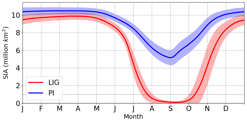
Figure 1Annual cycle of Arctic sea-ice area (SIA). The 200-year mean calculated from daily model output from 70–90∘ N for the LIG (red) and PI (blue) simulations is shown.
The earlier sea-ice retreat resulted in a warmer and less salty ocean surface during July, August, and September during the LIG (Figs. 2 and 3). The differences reached more than 5 ∘C (LIG–PI SST anomaly) and around 1–2 ppt for temperature and salinity respectively. The interaction of ocean surface conditions and sea-ice extent in the model simulations potentially allow sea surface temperature (SST) observations from proxy records to be used as a signature of ice conditions during the LIG. In particular it may be informative for the marine core community to search for large summer SST differences from the PI, of >4 ∘ C, at latitudes near the expected LIG ice edge (e.g. 70∘ N; east of Greenland) and smaller summer SST differences from the PI, of > 2 ∘C, in the central Arctic/Beaufort sea. This could help identify an sea-ice-free summer LIG Arctic in marine observations. However, we note that a partially-ice-covered summer Arctic, with thin LIG sea ice, might yield a similar signature to this but with lower magnitude temperature anomalies everywhere, as very thin summer ice cover has a small insulating effect (Serreze and Barry, 2011). Thus it is additionally useful to consider sea surface salinity (SSS) changes (Fig. 3). These have a clearer signature than SST. While the salinity patterns were similar in May for both simulations, the stronger melt during the LIG caused the region with LIG winter ice cover to become significantly fresher than the PI, by around 1–2 ppt in June and July. Additionally, a difference of 0.5–1.5 ppt was retained at least from March–September. Beyond helping identify the observational signature of a sea-ice-free Arctic, we aim to understand the following questions: what caused the large differences in summer sea ice in this model? Particularly, why did the spring melt increase so significantly in spite of the lower atmospheric CO2 concentration in the LIG? Processes with a significant impact on summer sea ice include thermodynamic processes such as ice–albedo feedbacks, ocean heat transport, and cloud cover feedbacks. Ice–albedo feedbacks may be significantly impacted by the presence of melt ponds, as discussed in Sect. 1. The preconditioning of winter sea ice may also lead to a reduced sea-ice extent the following summer (Parkinson and Comiso, 2013; Williams et al., 2016). In addition, summer sea-ice extent may be affected by changes to sea-ice distribution caused by changes to wind patterns and ocean circulation (Kageyama et al., 2021; Deser and Teng, 2008; Wang et al., 2009) further discussed in Sect. 3.1.1. It is currently unknown which process was most significant for the enhanced LIG sea-ice loss. We first look at the spin-up simulation for the LIG, with a particular focus on the first year of the spin-up (Figs. 4 and 5). Fig. 4 shows that the winter Arctic sea ice retained a similar area to the PI control period over the first 15 years of the spin-up period, beyond which it decreased only slightly (< 1 million square kilometres) from the PI control. However, an ice-free summer state was reached after only 4 years (Guarino et al., 2020b); we find August sea-ice area halved during the first year of the spin-up run from nearly 6 million to around 3 million square kilometres. Differences between PI and LIG developed rapidly during this first summer, within a few months of the January switch from PI to LIG forcings: this suggests that winter preconditioning did not play the dominant role in the enhanced melting of sea ice during the LIG spin-up. Similarly, this rapid loss of sea ice within the first few spin-up years cannot be explained by a change to ocean heat transport, which is often linked to reduced sea ice (Holland et al., 2006; Steele et al., 2010): upper ocean heat transport takes decades to equilibrate in numerical models after a significant perturbation, and deeper ocean heat transport takes centuries to millennia (Kantha and Clayson, 2000). Therefore, as can be seen from Fig. 4, changes to ocean heat transport could not have been the first-order driver of the rapid LIG sea-ice loss observed. Other factors that were present by the summer of LIG spin-up year 1 must be key to the enhanced melt throughout the simulated LIG period. In order to deduce the importance of two of the remaining processes, ice–albedo and cloud cover feedbacks, we consider the surface energy budget (Fig. 5). This is because the Arctic Ocean's surface heat balance is closely linked to its ice mass balance (Uttal et al., 2002; Untersteiner, 1961): at the surface, short-wave (SW) flux in particular is known to play a dominant role in summer sea-ice melt and is linked to ice–albedo feedbacks (Maykut and Perovich, 1987); longwave flux is related to the longwave cloud radiative forcing and cloud cover feedbacks (Gupta et al., 1992; Niemelä et al., 2001). Summer positive TOA radiation (Kageyama et al., 2021) led to a positive net absorbed SW flux anomaly, of up to 75 Wm−2 in June, that contributed nearly all of the net absorbed surface heat flux anomaly (Fig. 5a). Unlike changes related to preconditioning and ocean heat transport, this net SW flux anomaly was already present in the first year of LIG spin-up run, reaching 55 Wm−2 in June (Fig. 5b). This immediate response, coupled with the immediate halving of August sea-ice area, suggests the absorbed short-wave radiation played a key role in summer ice loss and thus that ice–albedo feedbacks may also have been important. We note also that the longwave anomaly accounted for < 5 Wm−2 of the total surface heat flux anomaly in Fig. 5b, so longwave forcings and feedbacks related to cloud cover were likely not dominant contributors to the enhanced LIG sea-ice loss, as confirmed by Guarino et al. (2020b). Other differences between the LIG and PI surface heat budget contributed < 20 Wm−2 monthly to the surface energy budget (Fig. 5). This suggests that thermodynamic processes that led to the enhanced LIG summer sea-ice melt must predominantly have resulted from this surface SW anomaly.
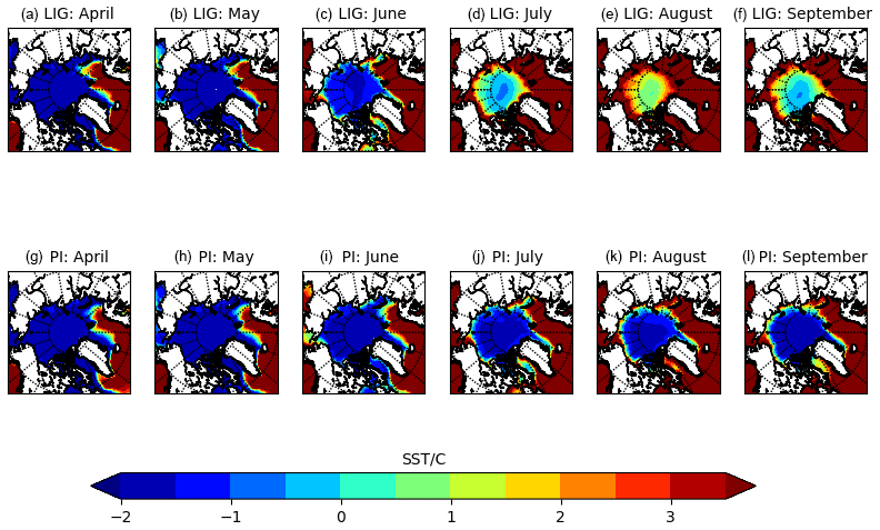
Figure 2Mean sea surface temperature (∘C) for the LIG and PI. The 200-year mean over the Northern Hemisphere for each month from April–September is shown, computed as the time average from monthly model output.
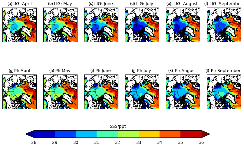
Figure 3Mean sea surface salinity (in parts per thousand, ppt) for the LIG and PI. The 200-year mean over the Northern Hemisphere for each month from April–September is shown, computed as the time average from monthly model output.
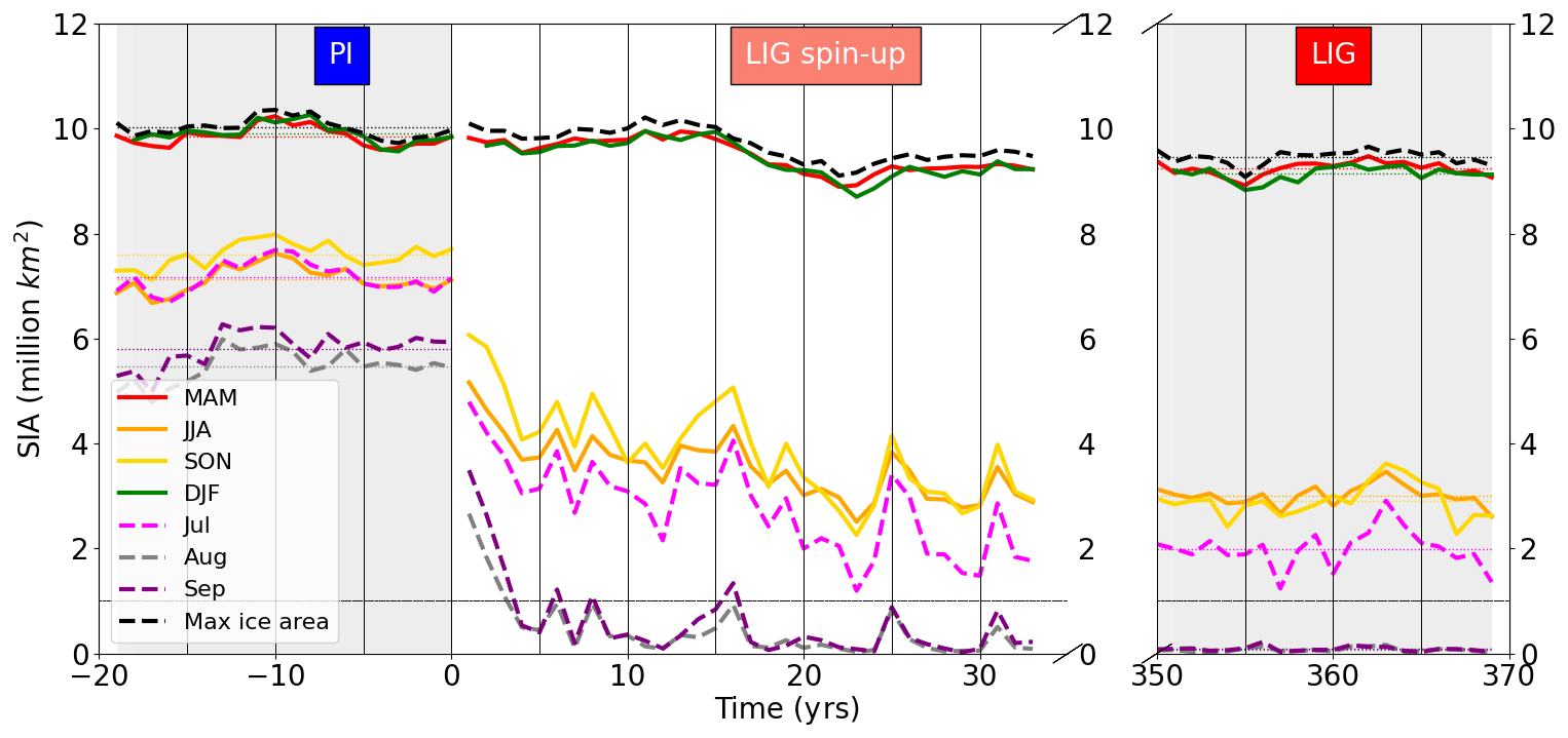
Figure 4The loss of Arctic sea-ice during the LIG spin-up. Comparison of seasonal Arctic sea-ice area (SIA) between simulated LIG and PI and first 35 years of LIG spin-up period, over the region 70–90∘ N, computed from monthly model output using ice-covered grid cells only. The black dashed line corresponds to maximum SIA reached any month during the year. A new ice-free state in August and September was reached within the first 5 years of the LIG spin-up.
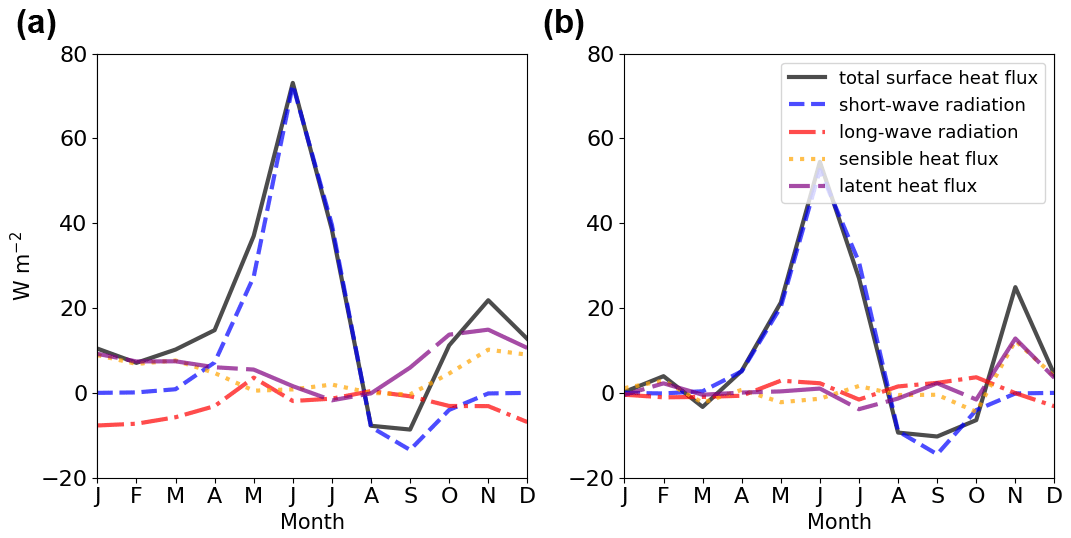
Figure 5Anomalies (LIG–PI) of the components of the surface energy budget from (a) the LIG simulation (adapted from Guarino et al., 2020b) and (b) the first year of LIG spin-up. For the LIG, PI, and the first year of the LIG spin-up period, the spatial average was computed from monthly data over the region from 70–90∘ N for the simulated short-wave radiation, long-wave radiation, sensible heat flux, and latent heat flux. For the LIG and PI periods, the 200-year mean was used. The total surface heat flux anomaly (black) is the sum of these four heat budget anomalies.
Therefore, by elimination, the dominant contributors to the enhanced LIG summer sea-ice loss were (i) thermodynamic processes, driven by this surface SW anomaly and likely related to ice–albedo feedbacks, and/or (ii) changes to the summer ice distribution. In the next section, we investigate the relative importance of these processes.

Figure 6Maps of mean simulated ice volume tendency (metres per month) due to thermodynamics for the LIG and PI. The 200-year mean over the Northern Hemisphere for each month from April–September is shown, computed as the time average from monthly model output.
3.1.1 Thermodynamic versus dynamic processes
Sea-ice increase and loss are driven by a combination of “thermodynamic processes”, which involve ice–atmosphere and ice–ocean heat fluxes, and “dynamic processes”, which involve changes to the local ice volume due to convergent or divergent ice motion (Li et al., 2014) caused by wind or ocean stress (Goosse and Fichefet, 1999). The key driver of ice motion is the wind stress forcing (Köberle and Gerdes, 2003): present-day interannual variability in Arctic summer sea-ice extent is linked to changes to sea-ice distribution caused by wind pattern variability due, for example, to large-scale atmospheric variability (Deser and Teng, 2008; Wang et al., 2009). In order to determine to what extent the enhanced LIG sea-ice loss was caused by these dynamic processes or by thermodynamic processes related to the SW anomaly shown in Fig. 5, we examine the ice volume tendencies due to thermodynamics and due to dynamics (both of which are primary model output variables). These are shown respectively in Figs. 6 and S4. The largest difference occurred in June, with 70 to 110 cm per month of ice melt during the LIG, in contrast to the 10 to 30 cm per month of ice melt in the PI simulation (Fig. 6). The thickness changes caused by dynamic processes (Fig. S4) were smaller. While a divergent ice drift reduced ice thickness during most months in the PI simulation, this was not the case during the LIG period. However, the differences in magnitude between the two periods were generally less than 10 cm per month. This demonstrates that, during spring and summer, changes in thermodynamic rather than changes in dynamic processes were the first-order driver causing increased ice melt for the LIG simulation. Thus, the SW anomaly shown in Fig. 5 was key to the enhanced LIG ice loss. Therefore, we investigate in the next section the source of this net absorbed SW anomaly at the surface.
3.1.2 Melt ponds and albedo feedback
At the ice surface, 20 %–30 % (Perovich et al., 2002a) of downwelling SW radiation is directly absorbed. Absorbed radiation may be transmitted through the ice to the ocean, which warms, leading to processes including further sea-ice melt (Perovich et al., 2002a). The ratio between downwelling and absorbed SW radiation is determined by the surface albedo. Sea ice has a high albedo and thus tends to predominantly insulate the ocean below it by reflecting most of the downwelling SW radiation. This can be seen from the similar spring SST under the PI and LIG Arctic sea ice (Fig. 2). Therefore, the LIG–PI TOA anomaly mentioned in Sect. 1 led to a downwelling surface SW flux anomaly, which in turn led to the anomaly of absorbed surface SW flux that is shown in Fig. 5. This absorbed anomaly may have been amplified (or reduced) by ice–albedo feedbacks that differed between the PI and LIG (Fig. 5). In this section, we investigate downwelling surface SW radiation and its amplification by ice–albedo feedbacks.
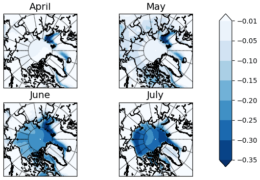
Figure 7The LIG–PI albedo difference. For both LIG and PI, the albedo for each grid cell was computed from monthly model output variables absorbed and downwelling short-wave flux. The LIG–PI anomaly is computed from the 200-year time averages for the PI and LIG.
We first consider the LIG–PI anomaly of the surface albedo in the Arctic Ocean. As can be seen from Figs. 7 and S5, this anomaly was small in April but grew throughout summer. The 5 % difference above 70∘ N in April grew, in July, to an average of −20 % and up to −35 % in some regions. Formation of melt ponds (which have lower albedos than sea ice) contributes to the albedo feedback effect (Perovich et al., 2002a; Hunke et al., 2015), so we evaluate the magnitude of the changes of pond evolution. As melt onset was not available as a model output variable, we use the mean first day each grid cell had a pond fraction greater than 1 % as a proxy for this. The geographical pattern of the first day of melt pond formation was similar for both periods, with ponds forming first at low latitudes and gradually spreading to higher latitudes (Fig. 8). Pond formation began on average 7.8 d earlier during the LIG compared to the PI. The difference between the two periods increases with latitude. Ponds south of 70∘ N began to form only 0–5 d earlier during the LIG than the PI. Ponds began to form at higher latitudes 15–20 d earlier during the LIG (Fig. 8c). As well as forming earlier in the LIG compared to the PI simulation, ponds also covered a greater area fraction of the ice-covered grid cells throughout the spring. For both periods, the long-term mean of the pond fraction of the grid cell for each month was greater for the LIG than the PI from May–June but smaller for the LIG than PI from July (Fig. 9). This is because melt ponds covered a larger area of the ice for the LIG than the PI in spring to early summer, but very little ice remained for the LIG simulation from July onwards, so there was less sea ice available for ponds to cover. Figure 10 shows the climatology of pond formation. At the end of April, the rate of pond formation was greater during the LIG than the PI; this initial increase is shown in more detail in Fig. S6. From early May, the total Arctic pond area increased exponentially with a rate of ∼ 0.14 d−1, until late May when the rate of pond formation began to decelerate; maximum pond area was reached in mid-June (Guarino et al., 2020b), which we compute as 2.67 ± 0.37 million square kilometres. For the PI, from early May, pond area increased exponentially with rate constant ∼ 0.09 d−1, until early June when the rate of pond formation decelerated until the maximum pond area was reached at 2.54 ± 0.45 million square kilometres in mid-July. A consistently higher fraction of the LIG sea ice was pond-covered throughout the spring, with a peak value of 45.3 ± 3.7 % (in early July) compared to peak value of 34.4 ± 5.1 % for the PI (in late July – not shown).
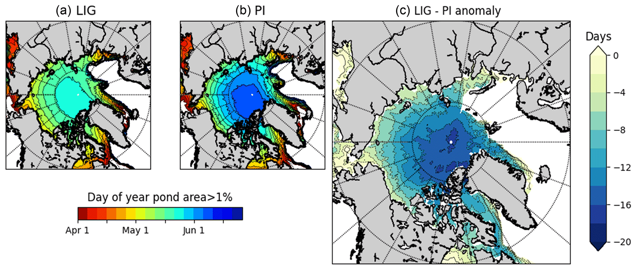
Figure 8First day of melt pond formation as proxy for melt onset. The mean day of the year the grid-cell melt pond fraction grew above 0.01 for (a) LIG, (b) PI, and (c) the LIG–PI anomaly. All figures show the 200-year mean from daily model output. Only grid cells still ice-covered when melt ponds began to form are shown.
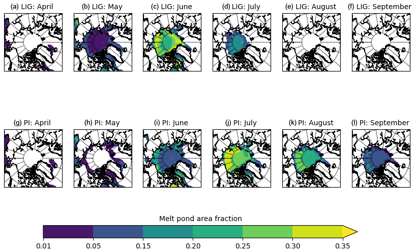
Figure 9Melt pond fraction. Monthly simulated melt pond fraction of the grid cell for LIG and PI. The 200-year mean over the Northern Hemisphere for each month from April–September is shown, computed as the time average from monthly model output.
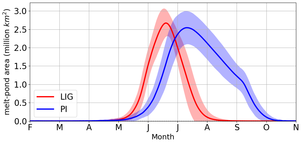
Figure 10Annual cycle of Arctic melt pond area. The 200-year mean was computed from the daily model output variables grid-cell sea-ice area and melt pond area over the region from 70–90∘ N. The shaded area is plus or minus twice the standard deviation. Only ice-covered grid cells were used.
In order to (i) compare downwelling SW radiation between the two time periods, (ii) quantify the importance of the albedo difference (Fig. 7), and (iii) characterise to what extent melt pond formation (Fig. 9) caused this albedo difference, we compare the downwelling with the absorbed SW radiation over ice-covered grid cells. To directly compare the same ice-covered geographical region between the PI and LIG simulations, for any given day of the year, all quantities are computed using only cells that were ice-covered on this day of the year in both simulations. The absorbed SW radiation was further broken down into the fraction absorbed by open water, by melt ponds, and by bare ice and snow, using their respective area fractions of the grid cell and estimating their respective albedos, as follows. For every grid cell for every day of model data, the mean surface albedo was calculated as described in Sect. 2.3. An open-water and pond albedo respectively of 0.07 and 0.27, alongside the area fraction of these two components for each cell (see Sect. 2.3), allowed the proportion of SW flux absorbed by each of these two components to be computed. The remainder of SW flux absorbed was attributed to exposed ice and snow. The change in surface albedo (due to changes in coverage of bare ice, snow, ponds, and open water) can be compared between the LIG and PI. For both time periods, north of the Equator, from January to June, the TOA downwelling SW flux increased. This increased the surface downwelling SW flux, which led to an increase in the absorbed SW flux. Figure 11a shows these changes in surface SW flux for the LIG: over ice-covered cells, an increase in downwelling flux from 96.8 ± 11.6 Wm−2 on 1 April to 312 ± 27 Wm−2 on 15 June led to the absorbed flux at the surface increasing from 24.0 ± 4.1 to 188 ± 27.4 Wm−2. Thus, from 1 April to 15 June, the LIG surface albedo decreased by 35 % (from 75 % to 40 %) over ice-covered regions. Similar computations for the PI (Fig. 11b) yield an albedo decrease of only 15 %. Thus, albedo changes were more significant for the LIG. In May, the gradient of the downwelling SW flux decreased, but the gradient of the absorbed SW flux increased, particularly for the LIG. This increasing rate of ice melt (see also Fig. 1), despite the slowing rate of change of downwelling solar radiation, implies that albedo feedbacks played an especially strong role in SW absorption through May during the LIG.
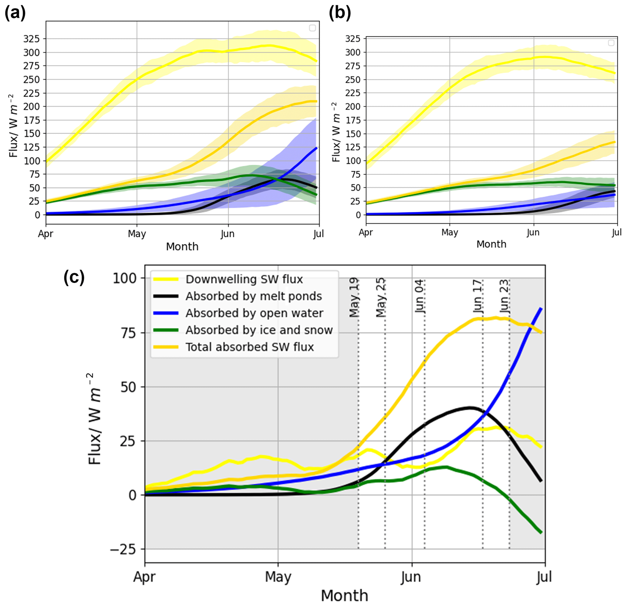
Figure 11Incident surface short-wave (SW) flux absorbed by each surface type. Calculated on ice-covered grid cells. (a) The LIG simulation (b) the PI simulation (c) anomaly of the LIG from the PI simulation. Figures show quantities calculated from the mean daily downwelling (yellow) and total absorbed (gold) SW flux at the surface, as well as the approximate breakdown of SW flux absorbed by open water (blue), exposed ice and snow (green), and melt ponds (black), all computed from daily model output from the first 50 years from each of the PI and LIG simulations. Further details in Sect. 3.1.2
Using Fig. 11c, we compare downwelling SW radiation between LIG and PI and use this to quantify to what extent albedo changes (related to albedo feedbacks) modified the surface absorbed SW anomaly shown in Fig. 5. Due to the TOA LIG–PI SW anomaly outlined in Sect. 1, the anomaly of the surface downwelling SW flux increased from 3.18 Wm−2 on 1 April to 29.9 Wm−2 on 15 June. This increased the anomaly of the absorbed SW radiation at the surface from 2.36 to 80.8 Wm−2, as seen from Fig. 11c. From Fig. 11c, it can be seen that the surface absorbed anomaly was 2.0 times the downwelling anomaly by 24 May, with a maximum of 4.61 times the downwelling anomaly on 4 June: the difference in surface albedo between the LIG and PI caused the difference in downwelling radiation to be amplified 4-fold. As the LIG–PI albedo difference increased so significantly from April through June, we have shown that the surface absorbed SW anomaly in Fig. 5a was caused by the TOA SW anomaly, very likely significantly amplified by stronger LIG than PI albedo feedbacks (as first suggested in Guarino et al. (2020b)).
Thus, for both time periods, from spring to summer: the radiative forcing triggered the albedo feedback, and the increase in the radiative forcing continued to strengthen this feedback into the summer. However, for the LIG, the stronger radiative forcing amplified the albedo feedback more significantly, so that a much greater fraction of the downwelling SW radiation was absorbed in the Arctic. This significantly changed the Arctic heat budget and ultimately resulted in a complete loss of Arctic sea ice by August.
Ice–albedo feedbacks result from changes in ice cover and pond formation. To determine to what extent melt pond formation (Fig. 9) impacted the albedo difference shown in Fig. 7 and caused the surface absorbed SW anomaly, we consider the LIG–PI anomaly of the SW radiation absorbed by each surface type. From Fig. 11c, it can be seen that the melt pond anomaly was comparable to the open-water anomaly from May to June and much greater than the ice and snow anomaly. In particular, from 19 May up until 23 June, just as the LIG–PI anomaly of the downwelling surface SW flux reached its peak, the magnitude of the melt pond anomaly was at least 0.5 times the open-water anomaly (and at least 1.4 times the ice anomaly). The melt pond anomaly from 25 May (at 15 Wm−2) to 17 June (at 38 Wm−2) was greater than both the open water anomaly and the ice and snow anomaly. Therefore, the role of melt ponds in decreasing the LIG albedo, thus amplifying the surface absorbed SW flux anomaly, was particularly significant as the surface downwelling SW flux anomaly grew through May and peaked in June. This demonstrates the significant impact of melt ponds on the surface energy balance and, by extension, their key role in enhancing LIG summer sea-ice loss.
3.2 Melt ponds and sea-ice predictability
Today's diminishing Arctic sea ice has led to a new focus on seasonal forecasting of Arctic sea-ice conditions and especially predicting the minimum sea-ice area each year (Williams et al., 2016). Spring melt ponds are a good predictor for summer sea-ice conditions (Schröder et al., 2014). It is of interest to see how the predictability of spring melt pond area and August–October sea-ice area varied between the PI and LIG, since this may yield insight into how predictability may change in future under conditions of reduced Arctic sea ice. Predictability is investigated here by considering interannual variability within each of the LIG and PI periods. The interannual variability in the radiative forcing at the surface was much smaller than the difference in the radiative forcing between the PI and LIG. Thus, investigating the relation between spring melt pond area and August–October sea-ice area within each of these two periods gives insight into the impact of melt ponds on the summer sea-ice area for similar TOA radiative forcing and winter ice conditions each year.
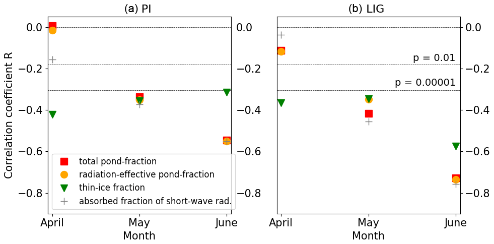
Figure 12Correlation between the spring melt pond fraction (MPF) of sea-ice area (SIA) and autumn SIA for (a) PI and (b) LIG. For both panels (a) and (b), 200 years of monthly model data were used over the region 70–90∘ N. Pearson's correlation coefficient R was calculated between mean August–October SIA and, in each of April, May, and June of the same year, (1) the mean pond fraction of sea-ice area (red), (2) the radiation-effective pond fraction (gold), (3) the mean thin-ice fraction of ice area (green), and (4) the mean fraction of incident short-wave radiation absorbed (grey). A statistically significant correlation is defined as correlation with p< 0.05; dotted lines delimit regions of very high statistical significance with p< 0.01 and p< 0.00001.
For the 200 years of simulation output for both LIG and PI, Pearson’s correlation coefficient was calculated between the mean August to October sea-ice area and each of the following four variables in each of April, May and June:
-
the mean monthly melt pond fraction;
-
the radiation-effective pond fraction, denoting the fraction of grid-cell area covered by ponds that are not covered by an ice lid and thus are expected to affect the surface albedo (Hunke et al., 2015);
-
the thin-ice fraction, defined as fraction of ice-covered grid cells with ice thickness <1.4 m, as the ice state in spring is known to affect the summer sea-ice area (Schröder et al., 2014);
-
the fraction of downwelling short-wave radiation absorbed, as this fraction over ice-covered cells accounts for albedo changes from open water as well as ponds in these cells.
Results are shown in Fig. 12. We note that, for both time periods, the April through June thin-ice fraction was a statistically significant () predictor of summer ice area, as might be expected (Schröder et al., 2014). However, of more interest here is the significance of the pond-related correlations through the spring. Whilst not significant in April for either period, by May, there was a significant negative correlation between melt pond formation and summer sea-ice area of −0.34 for the PI and −0.42 for the LIG. This is only a slightly weaker correlation than that of the absorbed short-wave fraction of −0.37 for the PI and −0.46 for the LIG (Fig. 12). By June both of these correlations were much stronger than the thin-ice fraction correlation: the melt pond correlation was −0.55 for the PI and −0.73 for the LIG, and the short-wave correlation was −0.55 for the PI and −0.76 for the LIG. These strong correlations show that spring melt pond formation alone was nearly as reliable a predictor of September ice cover as the presence of any water (including both ponds and open water) over ice-covered grid cells.
Compared to the PI, the LIG spring sea-ice area above 70∘ N was on the order of a million square kilometres lower, and the mean sea-ice thickness is about 1 m less. Therefore, the correlations shown in Fig. 12 imply that May–June pond-related quantities can be used to make more reliable seasonal predictions of summer sea ice for thinner (LIG) than thicker (PI) sea ice, as thinner ice is more sensitive to pond formation and albedo changes. This is of importance for future seasonal predictions: as the climate warms and Arctic sea ice continues to thin, the spring melt pond area is likely to become an increasingly reliable predictor of September sea-ice area.
3.3 Discussion
Despite their significant impact on sea-ice melt, melt ponds have only recently been explicitly included in global climate models (e.g. Collins et al., 2006; Curry et al., 2001). Prior to this, models without an explicit pond scheme had the ice albedo reduced when conditions approached near-melting (Hunke et al., 2015). Until now, it has not been clear whether this melt pond parameterisation approach adequately accounts for the impact of ponds during warmer-than-present-day conditions (Kwok et al., 2009).
Guarino et al. (2020b) found that HadGEM3 simulated an ice-free summer LIG Arctic and suggested this was linked to HadGEM3's realistic representation of melt pond physics. Here, we have quantified the importance of melt ponds during the LIG in depth, showing that greater melt pond formation, earlier in the year, directly led to the large surface energy budget difference between LIG and PI that was first highlighted in Guarino et al. (2020b). We have demonstrated the impact of melt ponds on thermodynamic processes during the LIG and their role in determining LIG spring albedo over ice-covered regions, leading to albedo feedbacks and ultimately the extreme ice loss first presented in Guarino et al. (2020b). Additionally, our analysis of the HadGEM3 PMIP4 LIG spin-up simulation years, showing that changes to longwave radiation and ocean heat transport were not primary drivers of the observed enhanced LIG ice loss, was supported by Guarino et al. (2020b), who used the LIG production run to show negligible differences in these factors between the simulated LIG and PI.
Of the CMIP6 models that have simulated the LIG according to CMIP6-PMIP4 experimental protocol, the two to include an explicit melt pond scheme are the two with the lowest minimum monthly SIA: HadGEM3, 0.2 million square kilometres, and CESM2, 1.2 million square kilometres (Kageyama et al., 2021). The only other model that simulated a minimum LIG SIA less than 2.0 million square kilometres was NESM3, at 1.3 million square kilometres. NESM3 has an unrealistic sea-ice representation for the PI period, with amplitude of the seasonal cycle and winter sea ice significantly overestimated (Kageyama et al., 2021); thus, we disregard this model in our analysis. For the remaining models which use parameterised rather than explicitly modelled ponds, the mean LIG minimum SIA was 3.5 ± 1.2 million square kilometres. Since only 16 models have run this simulation, it is not possible to say that implementing an explicit melt pond scheme will tend to result in lower simulated LIG summer ice area; other aspects of the model simulation set-up may also be significant in the simulation of Arctic sea ice. For example, the IPSL-CM6L model simulates some compensating ocean circulation and cloud cover changes that contribute to preserving LIG summer sea ice (Kageyama et al., 2021). However, despite these caveats, it is striking that the only two models to include explicitly modelled melt ponds also simulated minimum LIG SIA at least 2.3 million square kilometres less than (i.e. 1.9 standard deviations from) the mean of the models which use parameterised ponds, whilst simulating a realistic PI SIA annual cycle, as well as maximum LIG SIA similar to (i.e. 0.5 standard deviations from) the mean of the models which use parameterised ponds.
In terms of understanding mechanisms driving possible Arctic sea-ice change during the LIG, Guarino et al. (2020b) indicated that albedo changes were highly influential. Here we have provided a more in-depth follow-on study which analysed the potential thermodynamic and dynamic contributors and provided multi-model context that was not available to Guarino et al. (2020b). This shows that melt pond formation has a crucial impact on sea ice in warm climates, potentially making the difference between ice-covered and ice-free summer conditions. Specifically, we have answered the question of how HadGEM3's melt pond scheme contributed to the simulated ice loss in the Arctic during the LIG.
We have identified the key thermodynamic processes that led to the ice-free summer LIG Arctic as albedo feedbacks triggered by the radiative forcing. The TOA SW positive downwelling LIG–PI radiation anomaly in the spring and summer was halved by the time it reached the surface (Guarino et al., 2020b; Kageyama et al., 2021). However, we showed that the greater albedo feedback in the LIG compared to the PI (with LIG–PI surface albedo anomaly of < 5 % in April, growing to 30 %–35 % by July) amplified this small surface anomaly by the summer by a factor of 4. This meant up to 80 Wm−2 more short-wave radiation was absorbed at the surface, leading to significant differences between the LIG and PI surface heat budgets, and explaining the greatly enhanced LIG sea-ice melt compared to the PI. We further demonstrated that ponds played a key role in reducing the albedo and strengthening the feedback process: through May and June, the downwelling surface SW flux anomaly peaked, and over ice-covered cells, melt ponds and open water accounted for a similar proportion of the surface absorbed anomaly. Therefore, melt ponds contributed significantly to the simulated loss of summer sea ice.
Our analysis of ice volume tendencies demonstrated that the difference in HadGEM3-simulated LIG and PI summer ice melt rates was predominantly driven by thermodynamic processes. This is interesting since atmospheric and ocean circulation changes often contribute to ice loss (Li et al., 2014; Köberle and Gerdes, 2003; Kageyama et al., 2021; Goosse and Fichefet, 1999); however this was not the case here. We found that for both the PI and LIG, dynamic processes, driven by wind and ocean stress, led to less than 10 cm per month of Arctic ice volume change through the spring and summer months. By contrast, thermodynamic processes resulted in the most ice volume change for both simulations and accounted for the enhanced LIG ice loss. Three to 5 times more LIG sea ice was lost than during the PI by June in most Arctic regions: 70–110 cm per month of LIG sea ice was lost due to thermodynamic processes, compared to 10–30 cm per month during the PI.
Given today's new focus on seasonal forecasting of Arctic sea-ice conditions, and especially predicting the minimum sea-ice area each year (Williams et al., 2016), we also investigated whether melt ponds are a good predictor for summer sea-ice conditions (Schröder et al., 2014). Strong correlations between the May–June melt pond area and the August–October sea-ice fraction showed that explicitly modelling melt ponds significantly impacts the summer sea-ice area. Much stronger correlations were found for the LIG, which had thinner ice that was thus more sensitive to melt pond formation than the PI. This is of concern for future seasonal sea-ice predictions: as Arctic ice continues to thin, the spring melt pond area each year may be an increasingly important and reliable indicator of the September sea-ice area.
In conclusion, whilst both models with both parameterised and explicitly modelled melt ponds are relatively successful in representing present-day sea-ice behaviour (Collins et al., 2006; Curry et al., 2001; Flocco et al., 2012), we have found that they likely simulate significantly different sea-ice behaviour under forcings other than the present day. Multi-model context, alongside our new analysis above, suggests that a better representation of the contribution of melt ponds to enhanced Arctic sea-ice melt during the Last Interglacial is important. The relatively close match of HadGEM3 surface air temperatures to those derived from proxy records (Guarino et al., 2020b) and expected match of CESM2 (see figures in Otto-Bliesner et al., 2021) suggest that explicitly modelled pond formation for the LIG period does appear to be crucial to simulate realistic areas of summer sea-ice and Arctic temperature changes in current CMIP models. This is highly relevant to future projections of sea-ice loss, particularly when predicting the Arctic amplification of anthropogenic forcing; this requires accurate representation of albedo feedback mechanisms (Smith et al., 2019; Stuecker et al., 2018). Thus, our study of HadGEM3 supports the idea that an explicit, realistic melt pond scheme is required for both past and future sea-ice and climate projections.
The HadGEM3 model outputs prepared for CMIP6, including the simulated PI, are in the ESGF archive: https://doi.org/10.22033/ESGF/CMIP6.419 (Ridley et al., 2018a). Processed and additional HadGEM3 model outputs used in this study are available at http://gws-access.jasmin.ac.uk/public/pmip4/HADGEM3_LIG_PI/PUBLIC_DATA (Diamond and Guarino, 2021). The authors declare that all other data are available in the paper and its Supplement.
The supplement related to this article is available online at: https://doi.org/10.5194/tc-15-5099-2021-supplement.
RD conducted all analysis. LCS, DS, and MGV oversaw the direction and formulation of the research. MVG carried out the HadGEM3 simulations and supported the analysis of both simulations. DS guided the interpretation of all simulation results. All authors read the manuscript and provided comments. RD wrote the bulk of the manuscript with support from LCS and all other authors.
The authors declare that they have no conflict of interest.
Publisher’s note: Copernicus Publications remains neutral with regard to jurisdictional claims in published maps and institutional affiliations.
Rachel Diamond and Maria-Vittoria Guarino acknowledge support from NERC research grant NE/P013279/1. Louise C. Sime acknowledges support through NE/P013279/1, NE/P009271/1, and EU-TiPES. The project has received funding from the European Union’s Horizon 2020 research and innovation programme under grant agreement no. 820970. David Schroeder acknowledges support from the NERC-UKESM programme. This work used the ARCHER UK National Supercomputing Service (http://www.archer.ac.uk, last access: 16 February 2019) and the JASMIN data analysis platform (http://jasmin.ac.uk/, last access: 20 September 2021).
This research has been supported by the Natural Environment Research Council (grant nos. NE/P013279/1 and NE/P009271/1) and the Horizon 2020 research and innovation programme (TiPES, grant no. 820970).
This paper was edited by Thomas Mölg and reviewed by two anonymous referees.
Årthun, M., Eldevik, T., and Smedsrud, L. H.: The role of Atlantic heat transport in future Arctic winter sea ice loss, J. Climate, 32, 3327–3341, 2019. a
Auclair, G. and Tremblay, L. B.: The role of ocean heat transport in rapid sea ice declines in the Community Earth System Model Large Ensemble, J. Geophys. Res.-Oceans, 123, 8941–8957, 2018. a
Berger, A. and Loutre, M.-F.: Insolation values for the climate of the last 10 million years, Quaternary Sci. Rev., 10, 297–317, 1991. a
Bitz, C. M. and Lipscomb, W. H.: An energy-conserving thermodynamic model of sea ice, J. Geophys. Res.-Oceans, 104, 15669–15677, 1999. a
CAPE members: Last Interglacial Arctic warmth confirms polar amplification of climate change, Quaternary Sci. Rev., 25, 1383–1400, 2006. a
Collins, W. D., Bitz, C. M., Blackmon, M. L., Bonan, G. B., Bretherton, C. S., Carton, J. A., Chang, P., Doney, S. C., Hack, J. J., Henderson, T. B., Kiehl, J. T., Large, W. G., McKenna, D. S., Santer, B. D., and Smith, R. D.: The community climate system model version 3 (CCSM3), J. Climate, 19, 2122–2143, 2006. a, b, c, d
Curry, J., Schramm, J., Perovich, D., and Pinto, J.: Applications of SHEBA/FIRE data to evaluation of snow/ice albedo parameterizations, J. Geophys. Res.-Atmos., 106, 15345–15355, 2001. a, b, c, d
Curry, J. A., Schramm, J. L., and Ebert, E. E.: Sea ice-albedo climate feedback mechanism, J. Climate, 8, 240–247, 1995. a
Deser, C. and Teng, H.: Evolution of Arctic sea ice concentration trends and the role of atmospheric circulation forcing, 1979–2007, Geophys. Res. Lett., 35, L02504, https://doi.org/10.1029/2007GL032023, 2008. a, b, c
Diamond, R. and Guarino, M. V.: HadGEM3-GC3.1-LL lig127k and piControl processed outputs, [data set], available at: http://gws-access.jasmin.ac.uk/public/pmip4/HADGEM3_LIG_PI/PUBLIC_DATA/ last access: 20 September 2021. a
Eicken, H., Grenfell, T., Perovich, D., Richter-Menge, J., and Frey, K.: Hydraulic controls of summer Arctic pack ice albedo, J. Geophys. Res.-Oceans, 109, C08007, https://doi.org/10.1029/2003JC001989, 2004. a, b, c
Eyring, V., Bony, S., Meehl, G. A., Senior, C. A., Stevens, B., Stouffer, R. J., and Taylor, K. E.: Overview of the Coupled Model Intercomparison Project Phase 6 (CMIP6) experimental design and organization, Geosci. Model Dev., 9, 1937–1958, https://doi.org/10.5194/gmd-9-1937-2016, 2016. a
Fetterer, F. and Untersteiner, N.: Observations of melt ponds on Arctic sea ice, J. Geophys. Res.-Oceans, 103, 24821–24835, 1998. a, b
Fischer, H., Meissner, K. J., Mix, A. C., Abram, N. J., Austermann, J., Brovkin, V., Capron, E., Colombaroli, D., Daniau, A. L., Dyez, K. A., Felis, T., Finkelstein, S. A., Jaccard, S. L., McClymont, E. L., Rovere, A., Sutter, J., Wolff, E. W., Affolter, S., Bakker, P., Ballesteros-Cánovas, J. A., Barbante, C., Caley, T., Carlson, A. E., Churakova, O., Cortese, G., Cumming, B. F., Davis, B. A. S., De Vernal, A., Emile-Geay, J., Fritz, S. C., Gierz, P., Gottschalk, J., Holloway, M. D., Joos, F., Kucera, M., Loutre, M. F., Lunt, D. J., Marcisz, K., Marlon, J. R., Martinez, P., Masson-Delmotte, V., Nehrbass-Ahles, C., Otto-Bliesner, B. L., Raible, C. C., Risebrobakken, B., Sánchez Goñi, M. F., Saleem Arrigo, J., Sarnthein, M., Sjolte, J., and Valdes, P. J.: Palaeoclimate constraints on the impact of 2 C anthropogenic warming and beyond, Nat. Geosci., 11, 474–485, https://doi.org/10.1038/s41561-018-0146-0, 2018. a
Flocco, D., Feltham, D. L., and Turner, A. K.: Incorporation of a physically based melt pond scheme into the sea ice component of a climate model, J. Geophys. Res.-Oceans, 115, C08012, https://doi.org/10.1029/2009JC005568, 2010. a
Flocco, D., Schroeder, D., Feltham, D. L., and Hunke, E. C.: Impact of melt ponds on Arctic sea ice simulations from 1990 to 2007, J. Geophys. Res.-Oceans, 117, C09032, https://doi.org/10.1029/2012JC008195, 2012. a, b, c
Goosse, H. and Fichefet, T.: Importance of ice-ocean interactions for the global ocean circulation: A model study, J. Geophys. Res.-Oceans, 104, 23337–23355, 1999. a, b
Guarino, M.-V., Sime, L. C., Schroeder, D., Lister, G. M. S., and Hatcher, R.: Machine dependence and reproducibility for coupled climate simulations: the HadGEM3-GC3.1 CMIP Preindustrial simulation, Geosci. Model Dev., 13, 139–154, https://doi.org/10.5194/gmd-13-139-2020, 2020a. a
Guarino, M.-V., Sime, L. C., Schröeder, D., Malmierca-Vallet, I., Rosenblum, E., Ringer, M., Ridley, J., Feltham, D., Bitz, C., Steig, E. J., Wolff, E., Stroeve, J., and Sellar, A.: Sea-ice-free Arctic during the Last Interglacial supports fast future loss, Nature Climate Change, 1–5, 2020b. a, b, c, d, e, f, g, h, i, j, k, l, m, n, o, p, q, r, s, t, u, v, w, x
Gupta, S. K., Darnell, W. L., and Wilber, A. C.: A parameterization for longwave surface radiation from satellite data: Recent improvements, J. Appl. Meteorol., 31, 1361–1367, 1992. a
Holland, M. M., Bitz, C. M., and Tremblay, B.: Future abrupt reductions in the summer Arctic sea ice, Geophys. Res. Lett., 33, L23503, https://doi.org/10.1029/2006GL028024, 2006. a
Hunke, E. C., Lipscomb, W. H., Turner, A. K., Jeffery, N., and Elliott, S.: CICE: the Los Alamos Sea Ice Model Documentation and Software User’s Manual Version 5.1 LA-CC-06-012, T-3 Fluid Dynamics Group, Los Alamos National Laboratory, p. 116, 2015. a, b, c, d, e, f, g, h, i
IPCC: Climate Change 2013: The Physical Science Basis. Contribution of Working Group I to the Fifth Assessment Report of the Intergovernmental Panel on Climate Change, edited by: Stocker, T. F., Qin, D., Plattner, G., Tignor, M., Allen, S. K., Boschung, J., Nauels, A., Xia, Y., Bex, V., and Midgley, P. M., Tech. Rep. 5, Intergovernmental Panel on Climate Change, Cambridge, United Kingdom and New York, NY, USA, https://doi.org/10.1017/CBO9781107415324, 2013. a
Kageyama, M., Sime, L. C., Sicard, M., Guarino, M.-V., de Vernal, A., Stein, R., Schroeder, D., Malmierca-Vallet, I., Abe-Ouchi, A., Bitz, C., Braconnot, P., Brady, E. C., Cao, J., Chamberlain, M. A., Feltham, D., Guo, C., LeGrande, A. N., Lohmann, G., Meissner, K. J., Menviel, L., Morozova, P., Nisancioglu, K. H., Otto-Bliesner, B. L., O'ishi, R., Ramos Buarque, S., Salas y Melia, D., Sherriff-Tadano, S., Stroeve, J., Shi, X., Sun, B., Tomas, R. A., Volodin, E., Yeung, N. K. H., Zhang, Q., Zhang, Z., Zheng, W., and Ziehn, T.: A multi-model CMIP6-PMIP4 study of Arctic sea ice at 127 ka: sea ice data compilation and model differences, Clim. Past, 17, 37–62, https://doi.org/10.5194/cp-17-37-2021, 2021. a, b, c, d, e, f, g, h, i, j, k, l, m
Kantha, L. H. and Clayson, C. A.: Numerical Models of Oceans and Oceanic Processes, vol. 66, Academic Press, San Diego, 2000. a
Kay, J. E. and Gettelman, A.: Cloud influence on and response to seasonal Arctic sea ice loss, J. Geophys. Res.-Atmos., 114, D18204, https://doi.org/10.1029/2009JD011773, 2009. a
Köberle, C. and Gerdes, R.: Mechanisms determining the variability of Arctic sea ice conditions and export, J. Climate, 16, 2843–2858, 2003. a, b
Kuhlbrodt, T., Jones, C. G., Sellar, A., Storkey, D., Blockley, E., Stringer, M., Hill, R., Graham, T., Ridley, J., Blaker, A., Calvert, D., Copsey, D., Ellis, R., Hewitt, H., Hyder, P., Ineson, S., Mulcahy, J., Siahaan, A., and Walton, J.: The Low-Resolution Version of HadGEM3 GC3. 1: Development and Evaluation for Global Climate, J. Adv. Model. Earth Sy., 10, 2865–2888, 2018. a
Kwok, R., Cunningham, G., Wensnahan, M., Rigor, I., Zwally, H., and Yi, D.: Thinning and volume loss of the Arctic Ocean sea ice cover: 2003–2008, J. Geophys. Res.-Oceans, 114, C07005, https://doi.org/10.1029/2009JC005312, 2009. a, b
Li, L., Miller, A. J., McClean, J. L., Eisenman, I., and Hendershott, M. C.: Processes driving sea ice variability in the Bering Sea in an eddying ocean/sea ice model: anomalies from the mean seasonal cycle, Ocean Dynam., 64, 1693–1717, 2014. a, b
Lunt, D. J., Abe-Ouchi, A., Bakker, P., Berger, A., Braconnot, P., Charbit, S., Fischer, N., Herold, N., Jungclaus, J. H., Khon, V. C., Krebs-Kanzow, U., Langebroek, P. M., Lohmann, G., Nisancioglu, K. H., Otto-Bliesner, B. L., Park, W., Pfeiffer, M., Phipps, S. J., Prange, M., Rachmayani, R., Renssen, H., Rosenbloom, N., Schneider, B., Stone, E. J., Takahashi, K., Wei, W., Yin, Q., and Zhang, Z. S.: A multi-model assessment of last interglacial temperatures, Clim. Past, 9, 699–717, https://doi.org/10.5194/cp-9-699-2013, 2013. a
Lüthje, M., Feltham, D., Taylor, P., and Worster, M.: Modeling the summertime evolution of sea-ice melt ponds, J. Geophys. Res.-Oceans, 111, C02001, https://doi.org/10.1029/2004JC002818, 2006. a
Madec, G. and NEMO System Team: NEMO ocean engine, Scientific Notes of Climate Modelling Center, 27, ISSN 1288-1619, Institut Pierre-Simon Laplace (IPSL), Paris, 2015. a
Maslanik, J., Drobot, S., Fowler, C., Emery, W., and Barry, R.: On the Arctic climate paradox and the continuing role of atmospheric circulation in affecting sea ice conditions, Geophys. Res. Lett., 34, L03711, https://doi.org/10.1029/2006GL028269, 2007. a
Maykut, G. A. and Perovich, D. K.: The role of shortwave radiation in the summer decay of a sea ice cover, J. Geophys. Res.-Oceans, 92, 7032–7044, 1987. a
Menary, M. B., Kuhlbrodt, T., Ridley, J., Andrews, M. B., Dimdore-Miles, O. B., Deshayes, J., Eade, R., Gray, L., Ineson, S., Mignot, J., Roberts, C. D., Robson, J., Wood, R. A., and Xavier, P.: Preindustrial Control Simulations With HadGEM3-GC3. 1 for CMIP6, J. Adv. Model. Earth Sy., 10, 3049–3075, https://doi.org/10.1029/2018MS001495, 2018. a, b
Niemelä, S., Räisänen, P., and Savijärvi, H.: Comparison of surface radiative flux parameterizations: Part I: Longwave radiation, Atmos. Res., 58, 1–18, 2001. a
Otto-Bliesner, B. L., Rosenbloom, N., Stone, E. J., McKay, N. P., Lunt, D. J., Brady, E. C., and Overpeck, J. T.: How warm was the last interglacial? New model–data comparisons, Philos. T. R. Soc. A, 371, 20130097, https://doi.org/10.1098/rsta.2013.0097, 2013. a, b, c
Otto-Bliesner, B. L., Braconnot, P., Harrison, S. P., Lunt, D. J., Abe-Ouchi, A., Albani, S., Bartlein, P. J., Capron, E., Carlson, A. E., Dutton, A., Fischer, H., Goelzer, H., Govin, A., Haywood, A., Joos, F., LeGrande, A. N., Lipscomb, W. H., Lohmann, G., Mahowald, N., Nehrbass-Ahles, C., Pausata, F. S. R., Peterschmitt, J.-Y., Phipps, S. J., Renssen, H., and Zhang, Q.: The PMIP4 contribution to CMIP6 – Part 2: Two interglacials, scientific objective and experimental design for Holocene and Last Interglacial simulations, Geosci. Model Dev., 10, 3979–4003, https://doi.org/10.5194/gmd-10-3979-2017, 2017. a, b, c
Otto-Bliesner, B. L., Brady, E. C., Zhao, A., Brierley, C. M., Axford, Y., Capron, E., Govin, A., Hoffman, J. S., Isaacs, E., Kageyama, M., Scussolini, P., Tzedakis, P. C., Williams, C. J. R., Wolff, E., Abe-Ouchi, A., Braconnot, P., Ramos Buarque, S., Cao, J., de Vernal, A., Guarino, M. V., Guo, C., LeGrande, A. N., Lohmann, G., Meissner, K. J., Menviel, L., Morozova, P. A., Nisancioglu, K. H., O'ishi, R., Salas y Mélia, D., Shi, X., Sicard, M., Sime, L., Stepanek, C., Tomas, R., Volodin, E., Yeung, N. K. H., Zhang, Q., Zhang, Z., and Zheng, W.: Large-scale features of Last Interglacial climate: results from evaluating the lig127k simulations for the Coupled Model Intercomparison Project (CMIP6)–Paleoclimate Modeling Intercomparison Project (PMIP4), Clim. Past, 17, 63–94, https://doi.org/10.5194/cp-17-63-2021, 2021. a, b
Parkinson, C. L. and Comiso, J. C.: On the 2012 record low Arctic sea ice cover: Combined impact of preconditioning and an August storm, Geophys. Res. Lett., 40, 1356–1361, 2013. a
Perovich, D., Grenfell, T., Light, B., and Hobbs, P.: Seasonal evolution of the albedo of multiyear Arctic sea ice, J. Geophys. Res.-Oceans, 107, 8044, https://doi.org/10.1029/2000JC000438, 2002a. a, b, c
Perovich, D., Tucker III, W., and Ligett, K.: Aerial observations of the evolution of ice surface conditions during summer, J. Geophys. Res.-Oceans, 107, 8048, https://doi.org/10.1029/2000JC000449, 2002b. a
Perovich, D. K. and Tucker, W. B.: Arctic sea-ice conditions and the distribution of solar radiation during summer, Ann. Glaciol., 25, 445–450, 1997. a
Perovich, D. K., Light, B., Eicken, H., Jones, K. F., Runciman, K., and Nghiem, S. V.: Increasing solar heating of the Arctic Ocean and adjacent seas, 1979–2005: Attribution and role in the ice-albedo feedback, Geophys. Res. Lett., 34, L19505, https://doi.org/10.1029/2007GL031480, 2007. a
Ridley, J., Menary, M., Kuhlbrodt, T., Andrews, M., and Andrews, T.: MOHC HadGEM3-GC31-LL model output prepared for CMIP6 CMIP, Earth System Grid Federation [data set] https://doi.org/10.22033/ESGF/CMIP6.419, 2018a. a
Ridley, J. K., Blockley, E. W., Keen, A. B., Rae, J. G. L., West, A. E., and Schroeder, D.: The sea ice model component of HadGEM3-GC3.1, Geosci. Model Dev., 11, 713–723, https://doi.org/10.5194/gmd-11-713-2018, 2018b. a, b, c
Schröder, D., Feltham, D. L., Flocco, D., and Tsamados, M.: September Arctic sea-ice minimum predicted by spring melt-pond fraction, Nat. Clim. Change, 4, 353–357, 2014. a, b, c, d
Scott, F. and Feltham, D.: A model of the three-dimensional evolution of Arctic melt ponds on first-year and multiyear sea ice, J. Geophys. Res.-Oceans, 115, C12064, https://doi.org/10.1029/2010JC006156, 2010. a
Serreze, M. C. and Barry, R. G.: Processes and impacts of Arctic amplification: A research synthesis, Global and planetary change, 77, 85–96, 2011. a
Sime, L., Wolff, E., Oliver, K., and Tindall, J.: Evidence for warmer interglacials in East Antarctic ice cores, Nature, 462, 342–345, 2009. a
Skyllingstad, E. D., Paulson, C. A., and Perovich, D. K.: Simulation of melt pond evolution on level ice, J. Geophys. Res.-Oceans, 114, C12019, https://doi.org/10.1029/2009JC005363, 2009. a
Smith, D. M., Screen, J. A., Deser, C., Cohen, J., Fyfe, J. C., García-Serrano, J., Jung, T., Kattsov, V., Matei, D., Msadek, R., Peings, Y., Sigmond, M., Ukita, J., Yoon, J.-H., and Zhang, X.: The Polar Amplification Model Intercomparison Project (PAMIP) contribution to CMIP6: investigating the causes and consequences of polar amplification, Geosci. Model Dev., 12, 1139–1164, https://doi.org/10.5194/gmd-12-1139-2019, 2019. a
Steele, M., Zhang, J., and Ermold, W.: Mechanisms of summertime upper Arctic Ocean warming and the effect on sea ice melt, J. Geophys. Res.-Oceans, 115, C11004, https://doi.org/10.1029/2009JC005849, 2010. a
Stuecker, M. F., Bitz, C. M., Armour, K. C., Proistosescu, C., Kang, S. M., Xie, S.-P., Kim, D., McGregor, S., Zhang, W., Zhao, S., Cai, W., Dong, Y., and Jin, F.: Polar amplification dominated by local forcing and feedbacks, Nat. Clim. Change, 8, 1076–1081, 2018. a
Taylor, P. and Feltham, D.: A model of melt pond evolution on sea ice, J. Geophys. Res.-Oceans, 109, C12007, https://doi.org/10.1029/2004JC002361, 2004. a
Untersteiner, N.: On the mass and heat budget of Arctic sea ice, Arch. Meteor. Geophy. A, 12, 151–182, 1961. a
Uttal, T., Curry, J. A., McPhee, M. G., Perovich, D. K., Moritz, R. E., Maslanik, J. A., Guest, P. S., Stern, H. L., Moore, J. A., Turenne, R., Heiberg, A., Serreze, M. C., Wylie, D. P., Persson, O. G., Paulson, C. A., Halle, C., Morison, J. H., Wheeler, P. A., Makshtas, A., Welch, H., Shupe, M. D., Intrieri, J. M., Stamnes, K., Lindsey, R. W., Pinkel, R., Scott Pegau, W., Stanton, T. P., and Grenfeld, T. C.: Surface heat budget of the Arctic Ocean, B. Am. Meteorol. Soc., 83, 255–276, 2002. a
Walters, D., Boutle, I., Brooks, M., Melvin, T., Stratton, R., Vosper, S., Wells, H., Williams, K., Wood, N., Allen, T., Bushell, A., Copsey, D., Earnshaw, P., Edwards, J., Gross, M., Hardiman, S., Harris, C., Heming, J., Klingaman, N., Levine, R., Manners, J., Martin, G., Milton, S., Mittermaier, M., Morcrette, C., Riddick, T., Roberts, M., Sanchez, C., Selwood, P., Stirling, A., Smith, C., Suri, D., Tennant, W., Vidale, P. L., Wilkinson, J., Willett, M., Woolnough, S., and Xavier, P.: The Met Office Unified Model Global Atmosphere 6.0/6.1 and JULES Global Land 6.0/6.1 configurations, Geosci. Model Dev., 10, 1487–1520, https://doi.org/10.5194/gmd-10-1487-2017, 2017. a, b
Wang, J., Zhang, J., Watanabe, E., Ikeda, M., Mizobata, K., Walsh, J. E., Bai, X., and Wu, B.: Is the Dipole Anomaly a major driver to record lows in Arctic summer sea ice extent?, Geophys. Res. Lett., 36, L05706, https://doi.org/10.1029/2008GL036706, 2009. a, b, c
West, A. E., McLaren, A. J., Hewitt, H. T., and Best, M. J.: The location of the thermodynamic atmosphere–ice interface in fully coupled models – a case study using JULES and CICE, Geosci. Model Dev., 9, 1125–1141, https://doi.org/10.5194/gmd-9-1125-2016, 2016. a
Williams, C. J. R., Guarino, M.-V., Capron, E., Malmierca-Vallet, I., Singarayer, J. S., Sime, L. C., Lunt, D. J., and Valdes, P. J.: CMIP6/PMIP4 simulations of the mid-Holocene and Last Interglacial using HadGEM3: comparison to the pre-industrial era, previous model versions and proxy data, Clim. Past, 16, 1429–1450, https://doi.org/10.5194/cp-16-1429-2020, 2020. a
Williams, J., Tremblay, B., Newton, R., and Allard, R.: Dynamic preconditioning of the minimum September sea-ice extent, J. Climate, 29, 5879–5891, 2016. a, b, c
Williams, K., Copsey, D., Blockley, E., Bodas-Salcedo, A., Calvert, D., Comer, R., Davis, P., Graham, T., Hewitt, H., Hill, R., Hyder, P., Ineson, S., Johns, T. C., Keen, A. B., Lee, R. W., Megann, A., Milton, S. F., Rae, J. G. L., Roberts, M. J., Scaife, A. A., Schlemann, R., Storkey, D., Thorpe, L., Watterson, I. G., Walters, D. N., West, A., Wood, R. A., Woollings, T., and Xavier, P. K.: The Met Office global coupled model 3.0 and 3.1 (GC3. 0 and GC3. 1) configurations, J. Adv. Model. Earth Sy., 10, 357–380, 2018. a, b