Image classification of marine-terminating outlet glaciers in Greenland using deep learning methods

A wealth of research has focused on elucidating the key controls on mass loss from the Greenland and Antarctic ice sheets in response to climate forcing, specifically in relation to the drivers of marine-terminating outlet glacier change. The manual methods traditionally used to monitor change in satellite imagery of marine-terminating outlet glaciers are time-consuming and can be subjective, especially where mélange exists at the terminus. Recent advances in deep learning applied to image processing have created a new frontier in the field of automated delineation of glacier calving fronts. However, there remains a paucity of research on the use of deep learning for pixel-level semantic image classification of outlet glacier environments. Here, we apply and test a two-phase deep learning approach based on a well-established convolutional neural network (CNN) for automated classification of Sentinel-2 satellite imagery. The novel workflow, termed CNN-Supervised Classification (CSC) is adapted to produce multi-class outputs for unseen test imagery of glacial environments containing marine-terminating outlet glaciers in Greenland. Different CNN input parameters and training techniques are tested, with overall F1 scores for resulting classifications reaching up to 94 % for in-sample test data (Helheim Glacier) and 96 % for out-of-sample test data (Jakobshavn Isbrae and Store Glacier), establishing a state of the art in classification of marine-terminating glaciers in Greenland. Predicted calving fronts derived using optimal CSC input parameters have a mean deviation of 56.17 m (5.6 px) and median deviation of 24.7 m (2.5 px) from manually digitised fronts. This demonstrates the transferability and robustness of the deep learning workflow despite complex and seasonally variable imagery. Future research could focus on the integration of deep learning classification workflows with free cloud-based platforms, to efficiently classify imagery and produce datasets for a range of glacial applications without the need for substantial prior experience in coding or deep learning.

1 Introduction

Quantifying glacier change from remote sensing data is essential to improve our understanding of the impacts that climate change has on glaciers (Vaughan et al., 2013; Hill et al., 2017). In many glaciated areas, well-established semi-automated techniques such as image band ratio methods are used to extract glacier outlines for this purpose and to create glacier inventories (Paul et al., 2016). These methods are widely used in studies of mountain glaciers and ice caps (e.g. Bolch et al., 2010; Frey et al., 2012; Rastner et al., 2012; Guo et al., 2015; Stokes et al., 2018). However, they are less effective for mapping more complex glaciated landscapes such as marine-terminating outlet glaciers, which often contain spectrally similar surfaces like mélange (a mixture of sea ice and icebergs) near their calving fronts (Amundson et al., 2020).

As a result, manual digitisation remains the most common technique used to delineate marine-terminating glaciers (e.g. Miles et al., 2016, 2018; Carr et al., 2017; Wood et al., 2018; Brough et al., 2019; Cook et al., 2019; King et al., 2020). Nonetheless, the labour-intense nature of manual digitisation can result in datasets with spatial or temporal limitations (Seale et al., 2011). With this in mind, the importance of processes occurring at marine-terminating outlet glaciers on a range of spatio-temporal scales (Amundson et al., 2010; Juan et al., 2010; Chauché et al., 2014; Carroll et al., 2016; Bunce et al., 2018; Catania et al., 2018, 2020; King et al., 2018; Bevan et al., 2019; Sutherland et al., 2019; Tuckett et al., 2019) highlights the growing need for a more efficient method to quantify outlet glacier change, especially in an era of increasingly available satellite data.

To confront this challenge, several specialised automated techniques reliant on traditional image processing and computer vision tools (i.e. semantic segmentation and edge detection) have been developed to extract ice fronts in Greenland and Antarctica (Sohn and Jezek, 1999; Liu and Jezek, 2004; Seale et al., 2011; Krieger and Floricioiu, 2017; Yu et al., 2019). Semantic segmentation, a term interchangeable with pixel-level semantic classification, divides an image into its constituent parts based on groups of pixels of a given class and assigns each pixel a semantic label (Liu et al., 2019). It remains a core concept underlying more recent advancements which use deep learning approaches to classify imagery for more efficient automated calving front detection (Baumhoer et al., 2019; Mohajerani et al., 2019; Zhang et al., 2019; Cheng et al., 2021).

Deep learning is a type of machine learning in which a computer learns complex patterns from raw data by building a hierarchy of simpler patterns (Goodfellow et al., 2016). Convolutional neural networks (CNNs) are deep learning models specifically designed to process multiple 2D arrays of data such as multiple image bands (LeCun et al., 2015). They differ from conventional classification algorithms based solely on the spectral properties of individual pixels by detecting the contextual information in images such as shape and texture, in the same way a human operator would. This is beneficial for classification of complex environments with little contrast between spectrally similar surfaces (e.g. glacier ice/ice shelves, snow, mélange, and water containing icebergs) where traditional statistical classification techniques (e.g. maximum likelihood) produce more noisy classifications (Li et al., 2014). Previous studies which apply deep learning to detect the calving fronts of marine-terminating glaciers used a type of CNN called a fully convolutional neural network (FCN) (Ronneberger et al., 2015) and various post-processing techniques to extract the boundaries between (1) ice and ocean in Antarctica (Baumhoer et al., 2019) and (2) marine-terminating outlet glaciers and mélange/water in Greenland (Mohajerani et al., 2019; Zhang et al., 2019; Cheng et al., 2021). Calving fronts detected using these methods deviate by 38 to 108 m (<2 to 6 px) from manual delineations, providing an accurate automated alternative to manual digitisation.

These approaches have so far relied on a binary classification of input images. For example, Baumhoer et al. (2019) used only two classes (land ice and ocean). Similarly, Zhang et al. (2019) classified images into ice mélange regions and non-ice-mélange regions (the latter including both glacier ice and bedrock). While these methods are valuable for extracting glacier and ice shelf fronts to quantify fluctuations over time, they perhaps overlook the ability of deep learning methods to create highly accurate image classification outputs which contain more than two classes (i.e. not just ice and no-ice areas). Aside from calving front delineation, a method which produces multi-class image classifications could provide an efficient way to further elucidate processes and interactions controlling outlet glacier behaviour at high temporal resolution (e.g. calving events, the buttressing effects of mélange, subglacial plumes, and supra-glacial lakes). Moreover, deep learning has been used successfully in other disciplines to classify entire landscapes or image scenes to a high level of accuracy (Sharma et al., 2017; Carbonneau et al., 2020a). In glaciology, CNNs have been used to map debris-covered land-terminating glaciers (Xie et al., 2020), rock glaciers (Robson et al., 2020), supraglacial lakes (Yuan et al., 2020), and snow cover (Nijhawan et al., 2019). Despite this, multi-class image classification of entire marine-terminating outlet glacier environments has not yet been tested using deep learning.

Thus, the aim of this paper is to adapt a two-phase deep learning method which was originally developed to classify airborne imagery in fluvial settings (Carbonneau et al., 2020a) and test it on satellite imagery of marine-terminating outlet glaciers in Greenland. We first modify and train a well-established CNN using labelled image tiles from 13 seasonally variable images of Helheim Glacier, southeast Greenland. The two-phase deep learning approach is then applied to produce pixel-level classifications, from which calving front outlines are detected and error is estimated from manually delineated validation labels. We assess the sensitivity of the classification workflow to different image band combinations, training techniques, and model parameters for fine-tuning and transferability. Our objective is to establish and evaluate a workflow for multi-class image classification for glacial landscapes in Greenland which can be accessed and used rapidly without having specialised knowledge of deep learning or the need for time-consuming generation of substantial new training data. Furthermore, we aspire to exceed the current state of the art for pixel-level image classification of marine-terminating outlet glacier landscapes. The methods developed here are trained and tested on glaciers in Greenland with a pre-defined set of seven image classes.

2 Methods

2.1 Overview of CNN-Supervised Classification

The classification workflow used here is termed CNN-Supervised Classification (CSC) and was originally developed and tested on airborne imagery (<10 cm resolution) to produce pixel-level land cover classifications of fluvial scenes (Carbonneau et al., 2020a). CSC is a two-phase workflow based on convolutional architectures which concatenates a CNN to a multilayer perceptron (MLP) or compact CNN (cCNN). The two-phase approach was designed to simulate traditional supervised classification techniques (Carbonneau et al., 2020a). In effect, a pre-trained CNN is used in the first phase of CSC to produce locally specific training labels for each individual input image, replacing manual collection of training data which is typically required for traditional machine learning classifiers (Carbonneau et al., 2020a). The phase one CNN therefore accounts for image heterogeneity and incorporates the specific illumination conditions and seasonal characteristics of each unseen image by detecting local predictive features like brightness, texture, and geometry (e.g. crevasses) in relation to class. Thus, the predictions of the phase one CNN provide bespoke training labels for pixel-level image classification in phase two.

The pre-trained CNN applied in phase one of CSC falls into the category of supervised learning (Goodfellow et al., 2016) and is trained with a sample of image tiles which have been manually labelled according to class (training dataset). Each tile used to train the phase one CNN represents a sample of pure class (i.e. one class covers over 95 % of the tile area), allowing the CNN to learn predictive features and subsequently make class predictions for a tiled input image not previously seen in training (test dataset). During phase one of CSC, unseen test images are tiled and encoded in the form of 4D tensors which contain several separate tiles (dimensions: tiles, x dimension, y dimension, image bands). The pre-trained phase one CNN predicts a class for each input tile, and the tiles are subsequently re-assembled in the shape of the original input image (Fig. 1). As shown in Fig. 1, this produces a one band class raster made up of tiles, each of which is denoted by a single integer representing its predicted class. In phase two, the phase-one-predicted class raster and input image features are used to train a second model specific to the unseen input image. The predictions of this second model result in a final pixel-level image classification (Fig. 1).

Figure 1 Conceptual diagram of the CNN-Supervised Classification workflow showing the production of a tiled class raster in phase one. Phase one predictions are then used as image-specific training labels for the phase two model which produces a final pixel-level classification.

Since the phase one CNN predictions take the form of a tiled class raster, it is expected that individual tiles may straddle more than one class and result in inaccurate class boundaries. As a result, this will generate some error in the phase one predictions and therefore phase two training labels. Nonetheless, deep learning approaches have been found to tolerate noise in training labels (Rolnick et al., 2018). This is because the training process minimises overall error rather than memorising noise, meaning models can still learn a trend even if some labels are wrong. Likewise, the phase two models used in CSC are robust to noise and have been shown to overcome these errors with resulting pixel-level classifications following class boundaries much more accurately (Carbonneau et al., 2020a).

2.2 Study areas

2.2.1 Training area: Helheim Glacier, SE Greenland

An area spanning $\sim \mathrm{69}\times \mathrm{37}$ km (6875×3721 px) which includes Helheim Glacier (Fig. 2a), a major outlet of the southeastern Greenland Ice Sheet (GrIS), was chosen to adapt CSC for classification of marine-terminating outlet glacier landscapes and train the phase one CNN. Helheim is one of the five largest outlet glaciers of the GrIS by ice discharge (Howat et al., 2011; Enderlin et al., 2014) and has flow speeds of 5–11 km a⁻¹ (Bevan et al., 2012). The glacier has a 48 140 km² drainage basin (Rignot and Kanagaratnam, 2006) equivalent to ∼4 % of the ice sheet's total area (Straneo et al., 2016), from which several tributaries converge into a ∼6 km wide terminus. As shown in Fig. 2a, there is an extensive area of ice mélange adjacent to the terminus where it enters Sermilik Fjord and is influenced by ocean currents (Straneo et al., 2016). Inspection of available satellite imagery from 2019 revealed that the area of mélange varied seasonally with monthly variations in extension and composition as previously observed (Andresen et al., 2012, 2013).

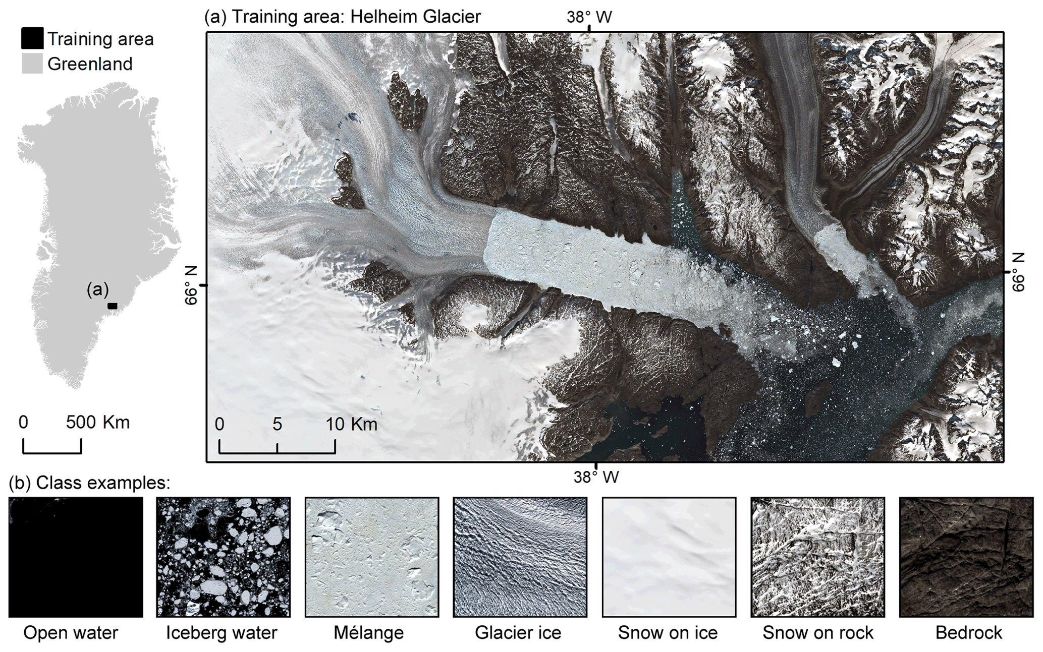
Figure 2 (a) Location of the area from which phase one CNN training data were extracted, showing Helheim Glacier (66.4^∘ N, 38.8^∘ W) and the surrounding landscape. Sentinel-2 image acquired on 15 June 2019. (b) Example image samples for each of the seven semantic classes used to train the phase one CNN. The outline of Greenland is from Gerrish (2020), and all Sentinel-2 imagery in this figure has been made available courtesy of the European Union Copernicus programme.

The glacier, fjord, and surrounding landscape provide an ideal training area for the deep learning workflow because they contain a number of diverse elements that vary over short spatial and temporal scales and are typical of other complex outlet glacier settings in Greenland. These characteristics include (1) seasonal variations in glacier calving front position; (2) weekly to monthly changes in the extent and composition of mélange; (3) sea ice in varying stages of formation; (4) varying volumes and sizes of icebergs in fjord waters; (5) seasonal variations in the degree of surface meltwater on the glacier and ice mélange; (6) short-lived, meltwater-fed glacial plumes which result in polynyas adjacent to the terminus; and (7) seasonal variations in snow cover on both bedrock and ice. The resulting spectral variations over multiple satellite images, in addition to potential differences resulting from changes in illumination and weather, pose a considerable challenge to image classification. However, capturing these characteristics at the scale of an entire outlet glacier image scene is important for a more efficient and integrated understanding of how numerous glacial processes interact. Examination of imagery showing the seasonal change of the glacial landscape throughout 2019 resulted in the establishment of seven semantic classes, including (1) open water, (2) iceberg water, (3) mélange, (4) glacier ice, (5) snow on ice, (6) snow on rock, and (7) bare bedrock (see class examples in Fig. 2b and detailed criteria for each in Table S1). Training and validation data for the phase one CNN applied in CSC was collected from the Helheim study area shown in Fig. 2 and labelled according to these seven classes.

2.2.2 Test areas: Helheim, Jakobshavn, and Store glaciers

The ability of a model to accurately predict the class of pixels in an unseen test image is called generalisation (Goodfellow et al., 2016) and determines the transferability of the model. To test the transferability of the CSC workflow adapted for marine-terminating glacial landscapes in Greenland, we applied CSC to a test dataset composed of seasonally variable imagery from in-sample and out-of-sample study sites (Fig. 3). CSC was never tested on any image that was used in training. Rather, the in-sample test dataset is compiled of images from the same glacier used in training but acquired on different dates to training data. The in-sample test site includes Helheim Glacier (Helheim) and has a slightly smaller area ($\sim \mathrm{47}\times \mathrm{40}$ km, or 4711×3986 px) compared to the training site (Fig. 3a).

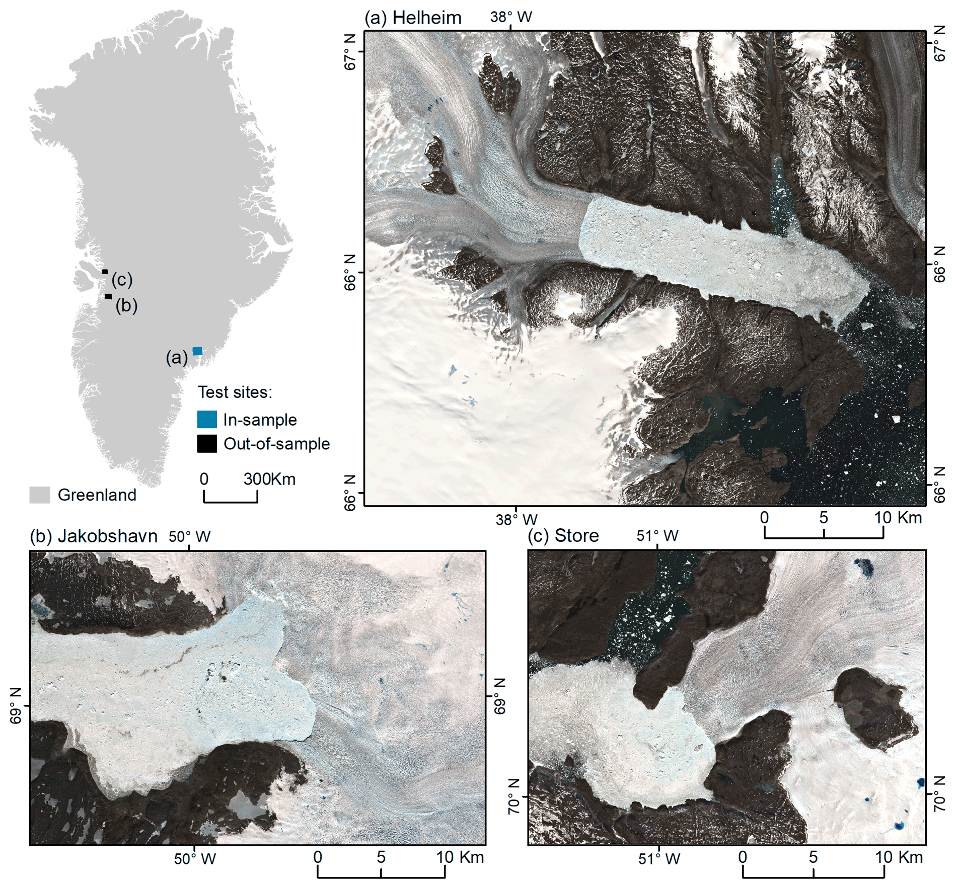
Figure 3 Test areas used to quantify the transferability of the CSC workflow. (a) The in-sample test area including Helheim Glacier. Example image acquired on 18 June 2019. (b) The out-of-sample test areas of Jakobshavn Isbrae (example image acquired on 21 May 2020) and (c) Store Glacier (example image acquired on 28 June 2020). The outline of Greenland is from Gerrish (2020), and all Sentinel-2 imagery in this figure has been made available courtesy of the European Union Copernicus programme.

The out-of-sample test areas contain Jakobshavn Isbrae (Jakobshavn) and Store Glacier (Store) in central west (CW) Greenland, and they represent outlet glacier landscapes never seen during training (Fig. 3b and c). The Jakobshavn site spans $\sim \mathrm{36}\times \mathrm{23}$ km (3566×2265 px) while the Store site spans $\sim \mathrm{28}\times \mathrm{21}$ km (2797×2089 px). Both out-of-sample test sites have notably different characteristics compared to the Helheim site, specifically in terms of glacier, calving front, and fjord shape, providing an adequate test of spatial transferability. Jakobshavn is the largest (by discharge) and fastest-flowing outlet of the GrIS (Mouginot et al., 2019). The glacier discharges 45 % of the CW GrIS (Mouginot et al., 2019) and has been undergoing terminus retreat, thinning, and acceleration over the past few decades (Howat et al., 2007; Joughin et al., 2008). As a result, the terminus of Jakobshavn is composed of two distinct branches which are no longer laterally constrained by fjord walls in the same manner as Helheim. Store Glacier is responsible for 32 % of discharge from the CW GrIS (Mouginot et al., 2019), but has remained relatively stable over the last few decades (Catania et al., 2018). The calving front of Store is laterally constrained by the walls of Ikerasak Fjord (Fig. 3c), and both Jakobshavn and Store glaciers have different flow directions in comparison to Helheim. The seven classes identified from the training area were also present in the out-of-sample test sites, including mélange which continuously occupied the fjord at Jakobshavn and was sporadically present in front of Store Glacier throughout the range of test imagery acquired in 2020 (Fig. 3).

2.3 Imagery

To train and test the CSC workflow, Sentinel-2 image bands 4, 3, 2, and 8 (red, green, and blue (RGB) and near infrared (NIR)) were used at 10 m spatial resolution. RGB bands are commonly selected for image classification with deep learning architectures, making existing CNNs easily transferable for the purpose of this study. Additionally, snow and ice have high reflectance in the NIR band, which is often used in remote sensing of glacial environments, for example to identify glacier outlines using band ratios (e.g. Alifu et al., 2015). Initial testing revealed that the combination of RGB and NIR bands (collectively referred to as RGBNIR) improved classification results compared to using RGB bands alone (see Sect. 2.6). Thus, four-band RGBNIR images of the study sites were used as CSC inputs.

Cloud cover and insufficient solar illumination present challenges when using optical satellite imagery such as Sentinel-2 data, meaning data availability for the study sites was limited to cloud-free imagery from February to October. Despite these limitations, sufficient data were available to train and test CSC on seasonal timescales. Therefore, to best encompass the seasonally variable landscape characteristics and collect sufficient training data to represent intra-class variation, 13 cloud-free Sentinel-2 images of the Helheim training area, taken between February and October 2019, were acquired for phase one CNN training (Table S2 in the Supplement). Similarly, a seasonally variable test dataset composed of nine in-sample images from 2019 with different dates to training data and 18 out-of-sample images from February to October 2020 were acquired (Table S2 in Supplement). Level-2A products were downloaded from Copernicus Open Access Hub (available at https://scihub.copernicus.eu/dhus/#/home, last access: 20 July 2020), and RGBNIR images were created, cropped to the study sites, and saved in GeoTIFF format. Additionally, a whole unseen Sentinel-2 tile (10 980×10 980 px) acquired on 13 September 2019 which included the entire landscape surrounding Helheim Glacier was used to test CSC over a larger spatial scale (i.e. more than a single glacier).

2.4 CSC model architectures and training

2.4.1 Phase 1: model architecture

For the base architecture of the pre-trained CNN used in phase one of CSC, we adapted a well-established CNN called VGG16 (Simonyan and Zisserman, 2015) which achieved state-of-the-art performance in the ImageNet Large Scale Visual Recognition Challenge (ILSVRC) 2014. The architecture used consists of five stacks of 13 2D convolutional layers which have 3×3 pixel filters (Fig. 4). The filter spatially convolves over the input image to create a feature map, using the filter weights. The dimensions of the output filters increase from 64 in the first stack of convolutional layers to 512 in the last (Fig. 4). All the convolutional layers use rectified linear unit (ReLU) activation and are interspersed with five max-pooling layers. The convolutional and pooling stacks are followed by three fully connected (dense) layers (i.e. a normal fine-tuned neural network) without shared weights, typical of CNN architectures. This section allows the features learned by the CNN to be allocated to a class by a final Softmax layer with the same number of units as classes. The Softmax layer, often used in multi-class models, determines the probability that an image tile is a member of each output class. It converts the outputs of the previous CNN layer to a probability distribution so the class with the highest probability of membership becomes the final class label for the respective image tile. The dense layers use L² regularisation to reduce over-training (Goodfellow et al., 2016; Carbonneau et al., 2020a).

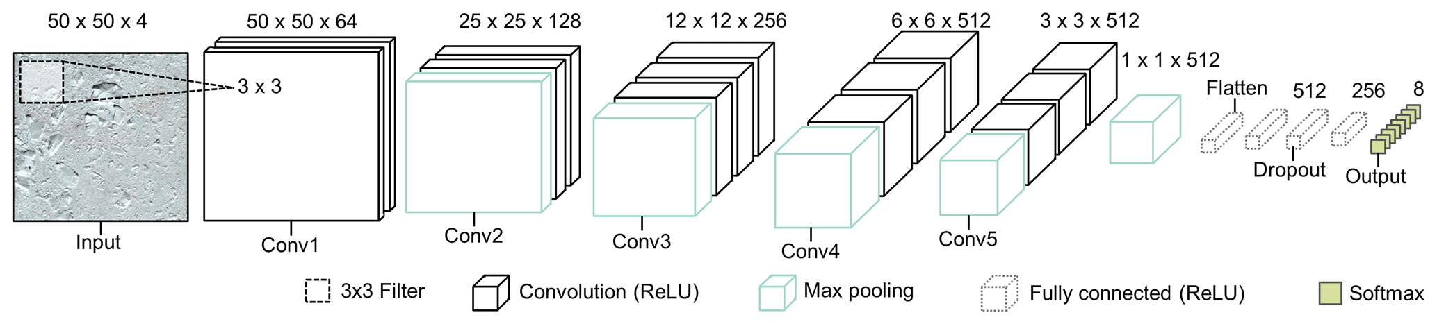
Figure 4 Architecture of phase one CNN, adapted from the original VGG16 model architecture (Simonyan and Zisserman, 2015). Diagram shows an example with a 50×50 px RGBNIR input image tile. There are five stacks of 2D convolutional layers (labelled “Conv#”) which extract features from input tiles using a 3×3 filter. The convolutional stacks are followed by a fully connected neural network and Softmax activation for phase one class prediction. The Sentinel-2 image in this figure is courtesy of the European Union Copernicus programme.

The input image tile size for the first convolutional layer in the original VGG16 model architecture was fixed as a $\mathrm{224}\times \mathrm{224}\times \mathrm{3}$ RGB image. However, here we tested the impact of tile size to determine the optimal scale for detecting features within the glacial landscape using 10 m resolution imagery. Tile sizes of 50×50, 75×75, and 100×100 px were tested, and architectures were adjusted accordingly (Fig. 4). Overall, optimal results in both phases of CSC were achieved using tile sizes of 50×50 px (see Sect. 2.6). Finally, since the input RGBNIR imagery has four bands, the number of input channels was adapted (i.e. from RGB in the original VGG architecture to RGBNIR in the adapted architecture).

2.4.2 Phase 1: model training

To train the phase one CNN, we employed early stopping to control hyperparameters and inhibit overfitting which occurs when a model is unable to generalise between training and validation data (Goodfellow et al., 2016). To do this, we designed a custom callback that trains the network until the validation data (20 % set aside with a train–validate–split) reach a desired target accuracy threshold. These targets ranged from 92.5 % to 99 % and determined the number of epochs the CNN was trained for. We used categorical cross entropy as the loss function and Adam gradient-based optimisation (Kingma and Ba, 2017) with a learning rate of $\mathrm{10}\times {\mathrm{10}}^{-\mathrm{4}}$ and batch sizes of 30.

When applying CSC to multiple sites, we came to a similar conclusion to Carbonneau et al. (2020a), who found that model transferability was improved when the phase one CNN was trained with data from more than one site. We therefore deployed a joint fine-tuning training procedure where a CNN initially trained only on data from Helheim was trained further with a small set of extra tiles (5000 samples per class) using only two images (one from winter and one from summer) for all three glaciers. This fine tuning was done at a low learning rate of $\mathrm{10}\times {\mathrm{10}}^{-\mathrm{5}}$ and smaller batch sizes of 10 in comparison to initial CNN training (which used a learning rate of $\mathrm{10}\times {\mathrm{10}}^{-\mathrm{4}}$ and batch size of 30). The rationale for this is that if a glacier is identified for monitoring, the addition of two available scenes to produce data used to fine-tune an existing CNN is not an onerous task and can deliver significant improvements to the final results. For clarity, we will refer to CNN training without this extra level of fine-tuning as “single” training and CNN training with this added fine-tuning as “joint” training. This resulted in an additional glacier-specific CNN with joint training for each of the three test areas.

2.4.3 Phase 1: training data production

A dataset of 210 000 training samples with 30 000 image tiles per class was used to train and validate the phase one CNN. To create the training tiles, the RGBNIR images extracted from 13 Sentinel-2 acquisitions were manually labelled according to the seven semantic classes using QGIS 3.4 digitising tools. Vector polygons labelled by class number were rasterised to produce a per-pixel class raster the same size as the training area. Both the input image and class raster were then tiled using a script which extracted tiles with high overlap using a stride of 20 px (Fig. 5). Each tile was extracted and assigned a class label based on the manually delineated class raster, and any tiles occupied by less than 95 % pure class were rejected, removing tiles containing mixed classes. Once extracted, each image tile was augmented by three successive rotations of 90^∘ (Fig. 5). Data augmentation is a common step for bolstering training datasets in deep learning and usually entails slightly altering existing data to increase the number of training samples (Chollet, 2017). Tile rotation also allows the model to learn classes which may appear at different orientations in unseen images, for example accounting for different glacier flow directions, providing the potential for increased transferability. Following augmentation, tiles were normalised by a constant value of 8192 to convert raw Sentinel-2 data to 16-bit floating point data. This was because a GPU with a Turing architecture was used in CNN training, enabling the use of the TensorFlow mixed precision training method for which the input is 16-bit floating point data.

Figure 5 Conceptual diagram of the tiling process used to create training and validation data. A specified tile size and stride were used to extract tiles from the class raster and training image. Image tiles were filtered, augmented, and saved to individual class folders using an $\mathrm{80}\mathit{\%}/\mathrm{20}\mathit{\%}$ split for training and validation data.

The tiles were randomly allocated to training and validation folders with an 80 %$/$20 % training–validation split for phase one CNN training. Overall, this resulted in a dataset upwards of 1 million tiles with a large imbalance that ranged from 50 000 tiles in class one to 900 000 tiles in class four. However, class imbalance can have negative impacts on model performance (Johnson and Khoshgoftaar, 2019), so 30 000 tiles were randomly subsampled from each class, thus drastically reducing the tile population and resulting in a balanced training dataset. The final number of 30 000 tiles per class was chosen after trial and error revealed that the CNN could be trained with all tiles loaded in an available RAM space of 64 GB with a 32 GB paging file. For the joint fine tuning of phase one CNNs, a small dataset of 5000 samples per class was extracted from a single winter image and a single summer image for each of the three glaciers.

2.4.4 Phase 2: model architectures and training

To classify airborne imagery of fluvial scenes at pixel level using the CSC workflow, Carbonneau et al. (2020a) applied a pixel-based approach using an MLP in the second phase of the workflow, achieving high levels of accuracy (90 %–99 %). We propose that applying pixel-based techniques to coarser-resolution imagery such as Sentinel-2 data may be less effective compared to applying the workflow to high-resolution imagery. Furthermore, particularly in landscapes containing marine-terminating glaciers, many distinct classes may be covered in snow or ice and therefore be very spectrally similar (i.e. all classes are white), and where this is the case a pixel-based MLP would predictably struggle to differentiate between classes. So, in addition to testing a pixel-based MLP, we adopted a patch-based approach which uses a small window of pixels to determine the class of a central pixel, as in Sharma et al. (2017). This approach is based on the idea that a pixel in remotely sensed imagery is spatially dependent and likely to be similar to those around it (Berberoglu et al., 2000). The use of a region instead of a single pixel allows for the construction of a small CNN (dubbed “compact CNN” or cCNN: Samarth et al., 2019) with fewer convolutional layers that assigns a class to the central pixel according to the properties of the region (Carbonneau et al., 2020b). It therefore combines spatial and spectral information. Sharma et al. (2017) use a patch size of 5×5 px for patch-based classification of medium-resolution Landsat 8 imagery. We tested both pixel- and patch-based approaches using an MLP and cCNN in the second phase of the workflow (the architectures and application of which are detailed in the following subsections “Multilayer Perceptron” and “Compact Convolutional Neural Network”). Specifically, five patch sizes of 1×1 (pixel-based), 3×3, 5×5, 7×7, and 15×15 px were tested. This revealed that larger patch sizes of 5×5 to 15×15 px delivered optimal classification results (see Sect. 2.6).

Multilayer perceptron

For the pixel-based classification in phase two, we used an MLP (Fig. 6a). An MLP is a typical deep learning model (also commonly known as an artificial neural network) which consists of three (or more) interconnected layers (Rumelhart et al., 1986; Berberoglu et al., 2000). The MLP has five layers consisting of four fully connected (dense) layers and one batch normalisation layer (Fig. 6a). The first dense layer has 64 output filters and is followed by a batch normalisation layer which helps to reduce overfitting by adjusting the activations in the network to add noise. This is followed by two more dense layers with 32 and 16 filters, respectively. Each dense layer uses L² regularisation and ReLU activation except the output layer. The final output layer in the network has Softmax activation and eight output filters for class prediction. We used categorical cross entropy as the loss function and Adam gradient-based optimisation (Kingma and Ba, 2017) with a learning rate of $\mathrm{10}\times {\mathrm{10}}^{-\mathrm{3}}$.

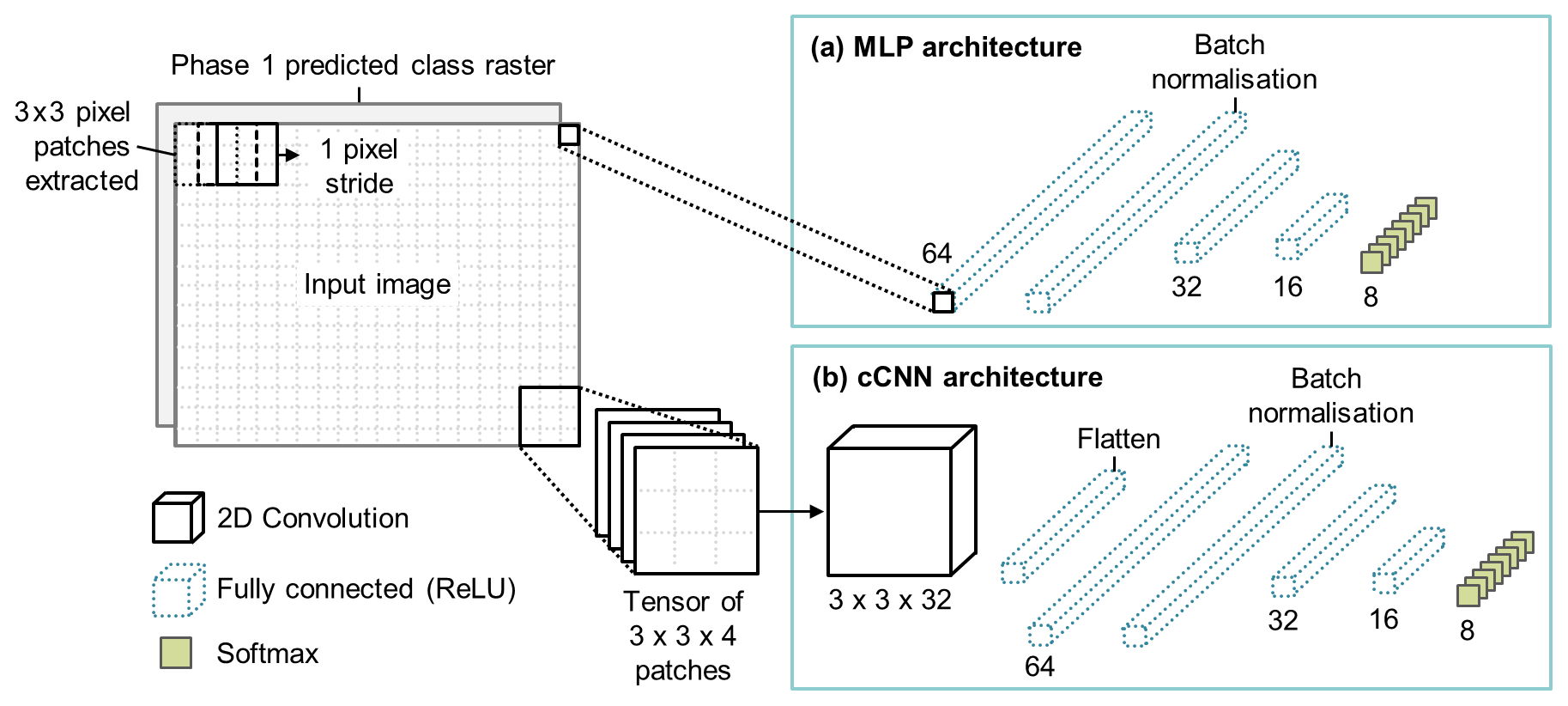
Figure 6 (a) Architecture of phase two multilayer perceptron used for pixel-based classification. (b) Architecture of the cCNN used in phase two for patch-based pixel-level classification. Patches are extracted from the input image with a stride of one pixel, assigned a class label according to the class raster produced in phase one, and compiled into 4D tensors which are then fed into the cCNN. An example of a 3×3 patch is shown in this diagram which uses an architecture with a single 2D convolutional layer with 32 3×3 filters. The convolutional layer feeds into a fully connected network like that of the MLP for class prediction.

The MLP was trained using conventional early stopping with a patience parameter and a minimum improvement threshold. The minimum improvement was set as 0.5 %. Training did not stabilise for at least 20 epochs, so the patience was set to 20. This means that if training does not improve the validation accuracy by 0.5 % after a period of 20 epochs, the training will stop. Since the MLP is pixel-based, the number of parameters was smaller compared to the patch-based model, with 3192 trainable parameters for RGBNIR imagery.

Compact convolutional neural network

For the patch-based classification in phase two, we used a cCNN architecture (Fig. 6b). This model architecture is referred to as a compact CNN (see Samarth et al., 2019) because it contains fewer convolutional layers in comparison to conventional CNNs. The cCNN learns the class of a central pixel in a patch as a function of its neighbourhood. So, for each pixel in the input image, a small image tile is extracted with square dimensions of the patch size (e.g. 3×3, 5×5, 7×7, or 15×15 px). The central pixel from the phase-one-predicted class raster is used as the associated class label. As with the phase one CNN, there are four input channels to match the number of bands, and the patches are fed into the cCNN in the form of 4D tensors (dimensions: patches, x dimension, y dimension, image bands).

The architecture of the cCNN is composed of a deepening series of convolution layers which change depending on the patch size. In effect, we use as many 3×3 filters as can be accommodated by the patch size without the recourse to padding. Therefore, for 3×3 image patches, we use a single 2D convolution layer since the convolution of a 3×3 image with a 3×3 kernel returns a single scalar value. An example of the cCNN architecture for a 3×3 px patch is shown in Fig. 6b. For the 5×5 image patch, we use two 2D convolution layers. The first convolution of the 5×5 image with a 3×3 kernel leaves a 3×3 image which is rendered to a scalar after a second 3×3 convolution. For the 7×7 image patch size, we use three 2D convolution layers. Finally, for the 15×15 patch size we use seven 2D convolution layers. In all cases, each convolution layer uses 32 filters and therefore passes 32 equivalent channels to the following layer, with the exception of the final layer which passes a set of 32 scalar predictors. These scalars are flattened and fed into a dense top which emulates the MLP architecture (Fig. 6a) and terminates in the usual Softmax layer for class prediction (Fig. 6b).

As with the MLP, conventional early stopping was used to train the cCNN with a patience parameter and a minimum improvement threshold. The minimum improvement was set as 0.5 %. For patch sizes of 3×3 we used a patience of 15, and for patches of 7×7 and 15×15 we used a patience of 10. The number of trainable of parameters reached up to 231 582 for RGBNIR imagery with a patch size of 15×15 px.

2.5 CNN-Supervised Classification performance

The performance of CSC was tested in two ways to allow comparison to previous deep learning methods. Firstly, classification accuracy was measured using manually collected validation labels. Secondly, a calving front detection method was implemented, and error was quantified using manually digitised calving front data for all test images.

Model performance is often measured by classification accuracy (the number of correct predictions divided by the total number of predictions). However, some models require more robust measures of accuracy which also account for confusion between predicted classes (Goodfellow et al., 2016; Carbonneau et al., 2020a). We therefore used an F1 score as the primary performance metric. The F1 score is defined as the harmonic mean between precision (p) and recall (r):

$$\begin{array}{}\text{(1)}& F\mathrm{1}={\displaystyle \frac{\mathrm{2}pr}{p+r}},\end{array}$$

where precision finds the proportion of positive predictions that are actually correct by dividing the number of true positives by the sum of both true (correct) positives and false (incorrect) positives. Recall finds the proportion of positive predictions that were identified correctly by dividing the number of true positives by the sum of true positives and false negatives (misidentified positives). Thus, the inclusion of recall provides a metric which represents confusion between class predictions (Carbonneau et al., 2020a). F1 scores range from 0 to 1, with 1 being equivalent to 100 % accuracy. Carbonneau et al. (2020a) used classification results from 862 images to compare F1 and accuracy. They found that they are closely correlated (accuracy $=\mathrm{1.03}F\mathrm{1}+\mathrm{4.1}$ % with an R² of 0.96), with F1 and accuracy converging at 100 %.

The validation labels used to calculate F1 scores were digitised manually using QGIS 3.4 digitising tools. Due to the manual nature of the data collection, this resulted in some unlabelled areas where classes were particularly difficult to define. This often occurred at class boundaries or where very small areas of different classes were mixed (at the scale of a few pixels). For example, in areas where the snow on rock class transitioned to bare bedrock, the structure of the underlying rock would often result in snow-covered areas spanning just a few pixels. In cases like this, digitising small patches of snow at pixel scale would be very time-consuming, and as a result some areas of the images remained unlabelled. Despite this, we aimed to cover as much of each test image with validation labels as possible.

F1 scores were calculated based on the concatenation of all the predictions for all available test images within the given parameters of tile size, patch size, number of bands, CSC phase, type of training (single or joint), glacier, and type of test data (in-sample or out-of-sample). Given that the calculation of F1 scores for gigapixel samples can be very computationally intensive, each F1 score presented here was estimated from a sample of 10 million pixels of the available data.

In addition to classification performance, we implemented a calving front detection method based on morphological geodesic active contours (see Fig. S1). The method is based on the definition of a calving front as the contact between “ocean” pixels (open water, iceberg water, or mélange) and glacier ice pixels. Since the final classification output from CSC is at pixel level, this allowed for calving front detection at the native spatial resolution of Sentinel-2 imagery (10 m). Error was quantified for each predicted calving front by measuring the Euclidean distance between each predicted calving front pixel and the closest pixel in manually digitised calving fronts. From this, the mean, median, and mode errors were quantified for each predicted calving front. Calculating the median and mode values allows the elimination of outliers in calving front predictions (Baumhoer et al., 2019). Calving fronts were digitised in QGIS 3.4 and rasterised to form a single pixel-wide line.

2.6 Optimal performance parameters

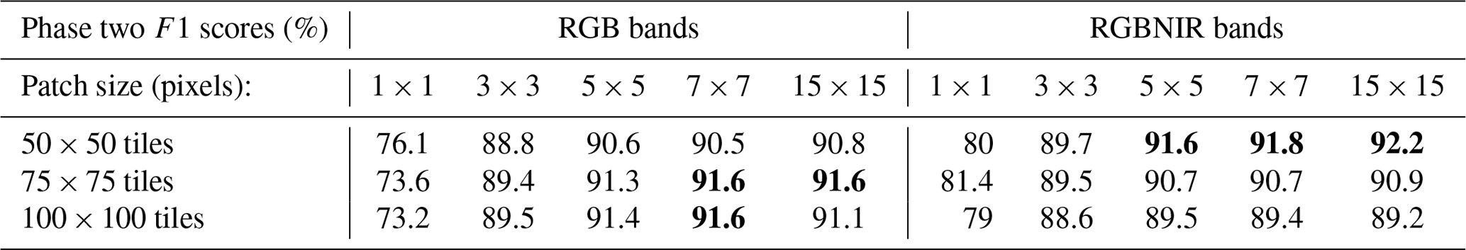
Table S3 shows that the highest classification performance in phase one was achieved using 50×50 px tiles from images composed of all four RGBNIR bands. For models trained with RGB bands, performance was highest with 100×100 px tiles, suggesting that the greater proportion of spatial information stored in larger tiles was beneficial when using only three bands. This finding extended to phase two results, and the additional testing of patch- vs. pixel- based techniques revealed that optimum classification performance was achieved using larger patch sizes from 5×5 to 15×15 px (Table 1) with F1 scores varying by only 0.6 % for classifications produced with 50×50 RGBNIR tiles.

Table 1 F1 scores for all test data combined (single training). The highest values are highlighted in bold. RGBNIR bands, 50×50 tiles, and the patch-based approach, specifically patches of 5×5 to 15×15 px, produced optimum classification results.

Similarly, an evaluation of calving front error for CSC results revealed that a patch size of 5×5 px produced the most accurate calving fronts, followed closely by patches of 7×7, 3×3, and 15×15 px (Fig. 7). Figure 7 shows the full error distribution for predicted calving front pixels detected from classifications produced with RGBNIR bands and 50×50 tiles. Overall, this suggests that optimum parameters for classification and calving front accuracy combined are 50×50 px RGBNIR tiles with a phase two patch size of 5×5 px. Using these parameters resulted in a mean calving front error of 56.17 m (equivalent to 5.6 px) for the test dataset as a whole (with individual mean errors of 58.81 m for Helheim, 70.6 m for Jakobshavn, and 39.1 m for Store). Additionally, median error was 24.7 m (equivalent to 2.5 px) for all test data (30 m for Helheim and Jakobshavn and 14.1 m for Store), and modal error was 10 m (equivalent to 1 px) for all glaciers, suggesting that mean values are increased by extremes.

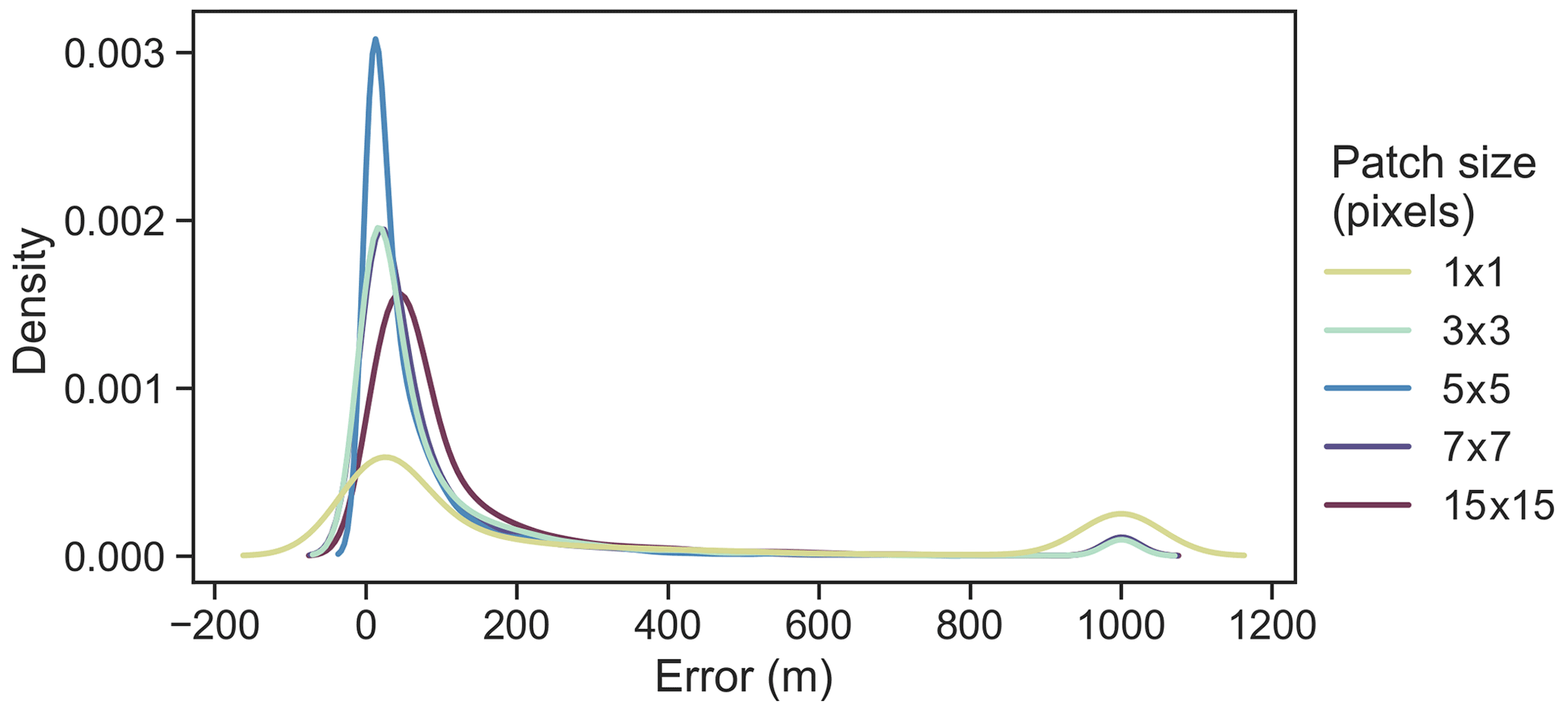
Figure 7 A kernel density estimate (KDE) plot of the full error distribution for all calving front predictions derived from all test sites using classifications produced with optimal parameters. Error values above 1000 m are grouped into a single bin to reduce tail length and show a second peak which represents catastrophic errors in calving front prediction. Note that low calving front errors occur most with 5×5 patches, followed by 7×7 and 3×3 patches, with the highest error occurring for the pixel-based approach.

In comparison, manually digitised calving fronts usually have an error of around 2 to 4 px. For example, Carr et al. (2017) calculated a mean calving front error of 27.1 m using repeat digitisations. In this work, small classification errors of a few pixels (often caused by shadows at the front) can lead to errors in the range of 5 to 10 px. The smaller-scale information provided in a 5×5 pixel patch is clearly optimal in comparison to overall classification accuracy, which achieves good results with patch sizes from 5×5 to 15×15 px. Furthermore, we note a small tail of data where large errors occurred (Fig. 7). The secondary peak in Fig. 7 represents calving front errors of 1000 m and above which shows where calving front predictions were catastrophically erroneous. This was caused by one of the 27 test images severely failing to detect the calving front (despite a high F1). The calving front error distribution derived from joint training can be found in Fig. S2.

3 Results

3.1 Classification performance

Figure 8 shows examples of CSC applied to images of the Helheim test site. High F1 scores are maintained despite the noticeable seasonal differences between images, such as changes in illumination, shadow, snow cover, ablation area, and mélange extent (Fig. 8a, c, and e). Corresponding calving front errors range from 10 to 42.4 m. Similarly, Fig. 9 shows examples of CSC applied to imagery of Store Glacier (out-of-sample). The F1 scores shown for the out-of-sample examples in Fig. 9 are slightly lower compared to the in-sample examples (Fig. 8). This is because the out-of-sample site is more prone to misclassification. For example, Fig. 9b shows several areas of glacier ice which have been misclassified as mélange. Additionally, in Fig. 9d there are areas of bedrock which are deeply shadowed, resulting in some misclassifications of bedrock areas as open water. These misclassifications did not increase calving front error, which ranged from 10 to 14.1 m (Fig. 9b, d, f), but lower F1 scores prompted testing of the joint fine-tuning method.

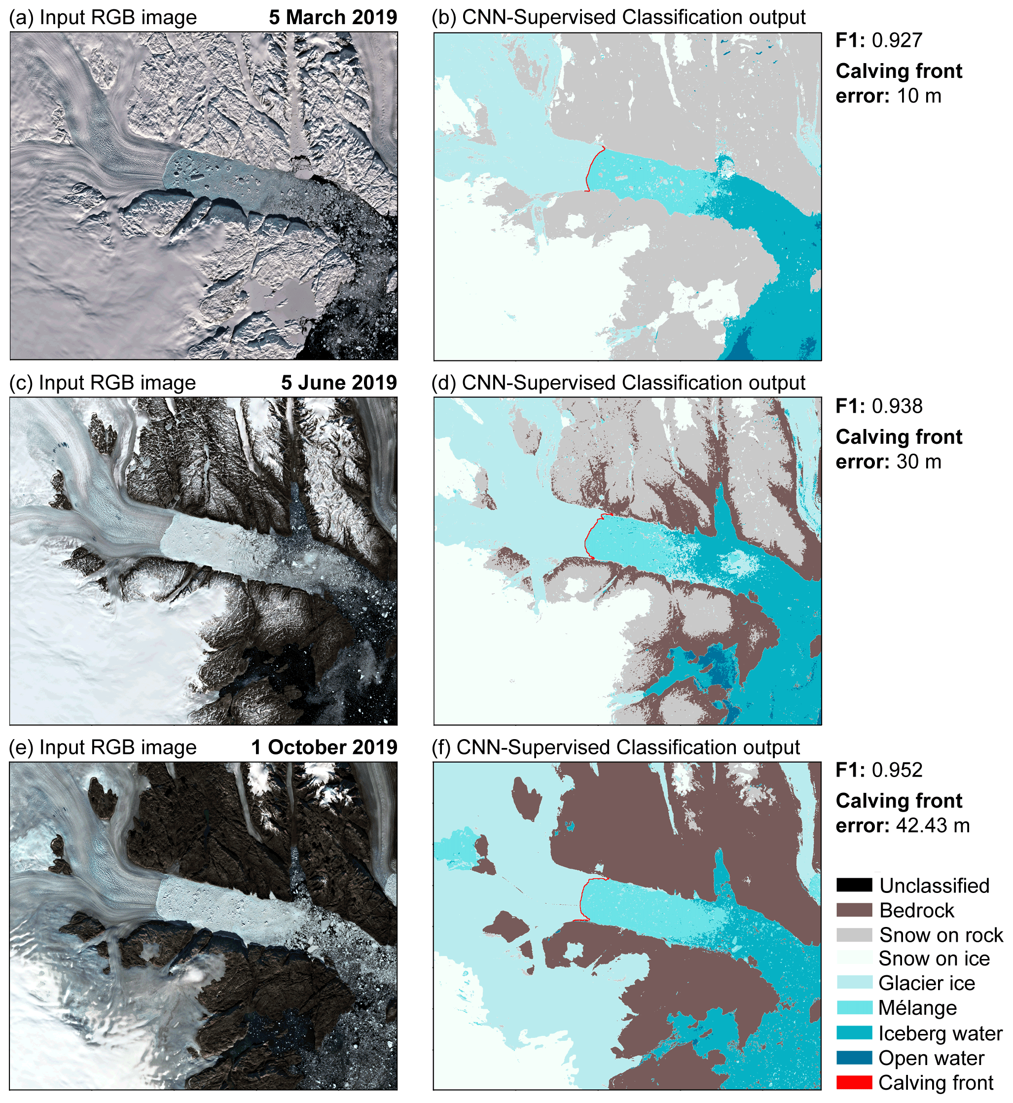
Figure 8 Examples of pixel-level classification outputs for seasonally variable imagery from the in-sample test site showing input images of Helheim in the first column, which were acquired on (a) 5 March 2019, (c) 5 June 2019, and (e) 1 October 2019 and the associated CSC outputs shown in (b), (d), and (f). Classifications produced using optimal parameters with F1 scores and calving front error shown next to each classification. All Sentinel-2 imagery in this figure is courtesy of the European Union Copernicus programme.

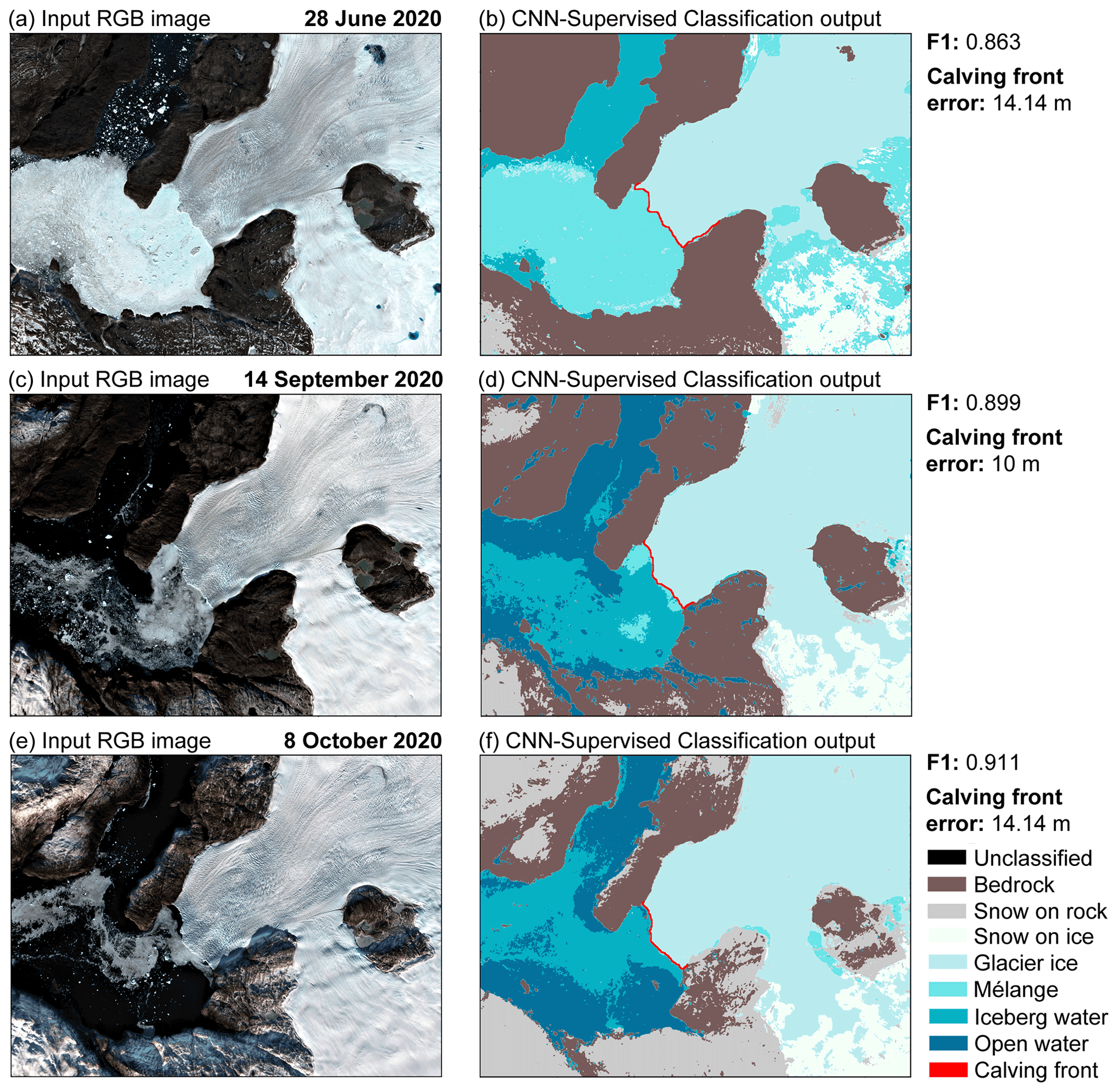
Figure 9 Examples of pixel-level classification outputs for seasonally variable imagery from the out-of-sample test site showing input images of Store in the first column, which were acquired on (a) 23 June 2020, (c) 14 September 2020, and (e) 8 October 2020 with the associated CSC outputs shown in (b), (d), and (f). Classifications produced using optimal parameters with F1 scores and calving front error shown next to each classification. All Sentinel-2 imagery in this figure is courtesy of the European Union Copernicus programme.

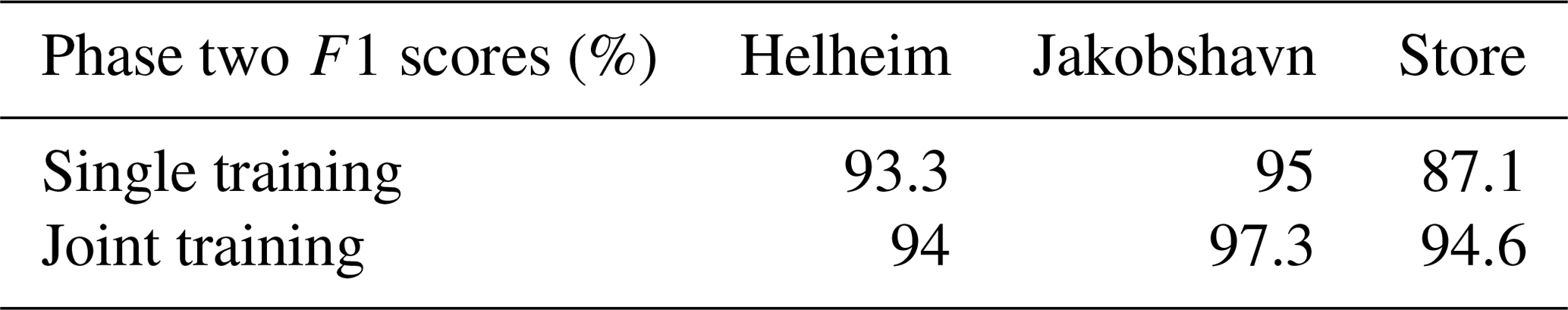
The joint training method improved classification performance (Table 2). Results were only marginally improved for the in-sample study site, which was to be expected since phase one models were already trained on data from Helheim. A comparison of classification outputs from single and joint training for an image of Store Glacier can be found in Fig. S3, which shows that the addition of joint fine-tuning rectified areas of misclassification seen in results which used single training, with the overall F1 score increasing from 84.7 % (single training) to 97.5 % (joint training). Figures S4 and S5 also show examples of joint training classifications. These examples suggest that digitising two additional images for the purposes of fine-tuning an existing pre-trained CNN for glacier-specific classification is worth the improvements in classification accuracy.

Table 2 Optimum F1 scores for classifications produced with single and joint training (50×50 RGBNIR tiles). Note the joint approach improves classification F1 scores, with the biggest improvement for out-of-sample sites.

Confusion matrices which show the relationship between CSC class predictions and validation data for each test glacier are shown in Fig. S6. In summary, Fig. S6 shows good agreement between predicted and actual classes for all glaciers, with the exception of the open water class for Helheim and Jakobshavn where confusion occurs between the iceberg water and bedrock classes. Open water is the smallest class for both sites, with open water often covering only small areas in each individual image. There is still class confusion in joint results (Fig. S7); however better overall F1 scores suggest that improvements are made in class prediction despite a different pattern of inter-class confusion. Overall, these examples show the ability of CSC to classify in- and out-of-sample imagery of marine-terminating glacial landscapes in Greenland with different seasonal characteristics.

Moreover, the size of input imagery to the CSC workflow is not limited to a specified set of dimensions. Since collection of validation labels for each test image required manual digitisation, the test sites were restricted to ∼20 to 50 km to allow collection of seasonal data for individual glacial landscapes. Despite this, CSC can also be applied to entire Sentinel-2 tiles. The outputs of the CSC workflow applied to an entire Sentinel-2 image are shown in Fig. S8. The overall F1 score of this classification was 92 %. This suggests that CSC has good classification performance at the level of individual glaciers as well as whole glacial landscapes.

3.2 Time series of Helheim Glacier

A time series produced using CSC results showing calving front position and changes in mélange area at Helheim throughout 2019 can be seen in Fig. 10. Figure 10a and c show fluctuation in calving front position between March and October 2019 with an overall pattern of retreat. Two predicted calving fronts which had an error of over 4.2 px were removed from the time series, and frontal position change was quantified using the rectilinear box method to account for cross-glacier variation (Lea et al., 2014). Figure 10b and c illustrate the variation in mélange area for all nine in-sample test images. Taken together, these results show the robustness of CSC and usefulness of multi-class outputs for holistic analysis of marine-terminating glacial environments.

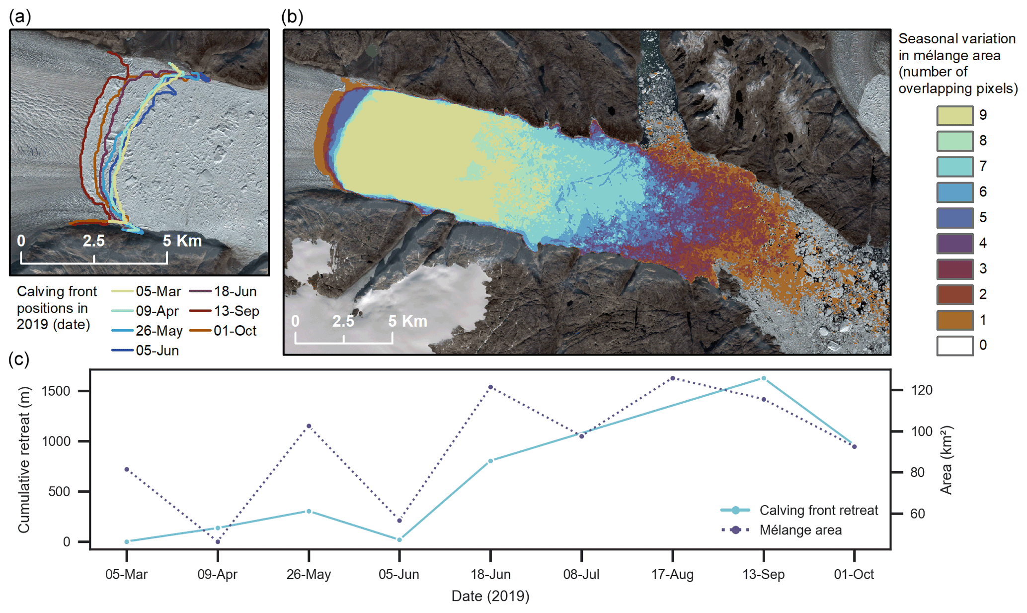
Figure 10 (a) Time series of Helheim calving front positions produced from CSC outputs of the 2019 test data. (b) Frequency of CSC-predicted mélange pixels from the Helheim test dataset showing the seasonal variation in mélange extent. (c) Cumulative retreat of the calving front relative to 5 March 2019 and mélange area for each test image. All background Sentinel-2 imagery in this figure has been made available courtesy of the European Union Copernicus programme.

4 Discussion

4.1 Comparison to previous work

Our results build on the work of deep-learning-based classification methods for ice front delineation (Baumhoer et al., 2019; Mohajerani et al., 2019; Zhang et al., 2019; Cheng et al., 2021), with several key innovations and variations of note. Firstly, the CSC workflow produces multi-class outputs using seven semantic classes rather than the binary outputs of previous methods. This fulfils the aim to provide meaningful information which could be used for a variety of applications at the scale of entire outlet glacier landscapes. In terms of classification accuracy, CSC produces marginally better F1 scores in comparison to previous methods applied to marine-terminating glacial environments. Previous studies which focus on outlet glaciers of the GrIS do not provide F1 scores for their classification outputs. However, Baumhoer et al. (2019) apply their method to Antarctic marine-terminating environments and produce overall F1 scores of 89.5 % for training areas (in-sample) and 90.5 % for test areas (out-of-sample). In comparison, CSC produces F1 scores of up to 93.3 % for in-sample test imagery and 91 % for out-of-sample test imagery when using a phase one CNN trained only with data from Helheim Glacier. By applying joint CNN training to fine-tune the phase one CNN to each test glacier, F1 scores increased to 94 % for in-sample test data and 96 % for out-of-sample test data. It is worth noting that the characteristics of Antarctic outlet glacier environments can vary substantially from Greenlandic outlet glacier environments, potentially presenting different classification challenges. As such, this is a tentative comparison, especially given that CSC outputs contain seven classes at the scale of the whole landscape, rather than just two classes focused at the ice front.

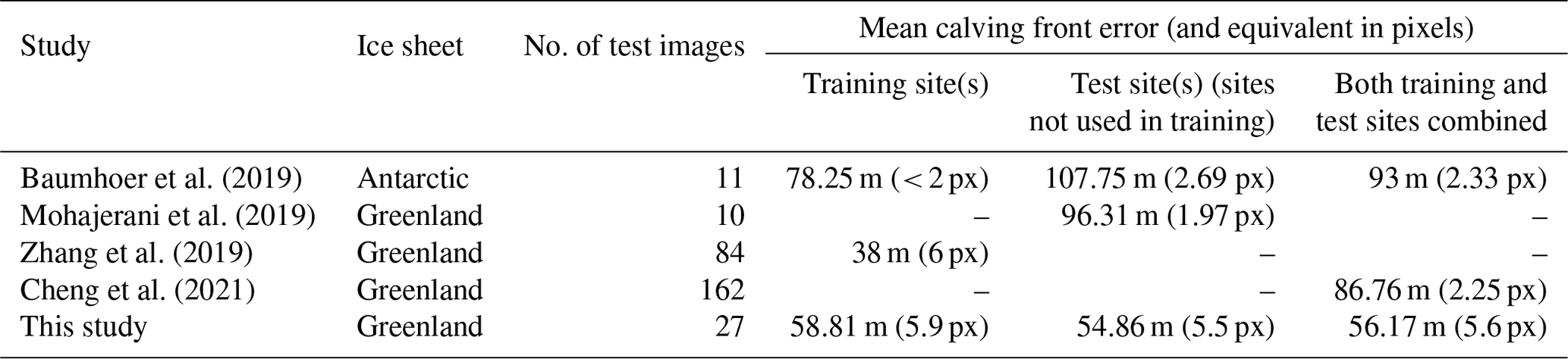
Additionally, since previous deep learning studies which produce binary classifications for Greenlandic outlet glaciers do not provide F1 scores, for further comparison we integrated a calving front detection method into the CSC workflow. Table 3 shows the mean calving front errors produced in this study and each of the previous studies. Mean calving front errors for test imagery from both training sites (in-sample) and test sites (out-of-sample) are provided; however not all studies specified these values. In terms of the number of metres that predicted fronts deviate from manual digitisations, the predictions of CSC are comparable to those of previous studies. However, in terms of the equivalent number of pixels, CSC predictions deviate from manual digitisations by a few more pixels compared to previous studies (apart from Zhang et al., 2019), indicating that if a given application solely requires accurate calving front localisation of a known glacier, the method presented here is not necessarily the optimal choice.

Table 3 Mean calving front errors from previous deep learning methods designed specifically to detect ice fronts in comparison to the mean calving front errors produced by CSC in this study.

The second major difference between CSC and previous methods is the deep learning architecture. All previous deep learning classification methods for delineating ice fronts (Baumhoer et al., 2019; Mohajerani et al., 2019; Zhang et al., 2019; Cheng et al., 2021) use FCN/U-Net architectures (Ronneberger et al., 2015). Hoeser et al. (2020) reviewed image segmentation and object detection in remote sensing, and whilst they do conclude that FCN/U-Net architectures are dominant, they still find about 30 % of published work uses patch-based approaches which are akin to the second phase of the CSC method presented here. This suggests that FCN architectures need not be considered the de facto algorithm for glacial landscape classification. Moreover, the advantage of CSC over one-stage patch-based methods using FCNs is that the initial phase one CNN provides transferability and delivers bespoke training labels for the pixel-level patch-based operator (as described in Sect. 2.1). We discuss the other major implications of the architectural differences between our work and FCNs in the following sections.

4.1.1 Data pre-processing and computational loads

CSC has certain practical advantages over FCNs in terms of data processing and computational loads. Firstly, the CSC method has low pre-processing requirements. In effect, Sentinel-2 images were cropped to produce large images containing whole marine-terminating glacier landscapes, yet still within a workable size for detailed digitisation of validation labels. The only other pre-processing step required is normalisation by a constant factor of 8192 to convert raw Sentinel-2 data to 16-bit floating point data. Once this is done, CSC has a low computational load. Training the initial VGG16 model can be done in under 1 h using an I7 processor at 5.1 GHz and an Nvidia RTX 2060 GPU. When CSC is subsequently applied to a sample image of $\sim \mathrm{3000}\times \mathrm{3000}$ px using optimal phase one parameters and a phase two patch size of 7×7 px, classification requires 4 min. We also coded a low-memory-usage pathway in the main script that classifies a large image row by row with a threshold to define “large” set by the user. Using this, Sentinel-2 images can be classified at native resolution (10 980×10 980 px each) in 12 min with a peak RAM consumption of 11 GB. This makes CSC suitable for use in free cloud-based solutions such as Google Colaboratory, providing the potential to build on existing cloud-based tools for glacial mapping (e.g. Lea, 2018). Moreover, given the simplicity of data pre-processing steps required for CSC, the workflow has good accessibility and can be implemented easily by new users.

In contrast, for several of the previous studies which implement FCN architectures, a larger number of pre-processing steps are required, including but not limited to rotation for consistent glacier flow direction, edge enhancement, and pseudo-HDR toning (Mohajerani et al., 2019; Zhang et al., 2019; Cheng et al., 2021). Similarly, FCN architectures can be very demanding in terms of computer RAM and GPU RAM, especially when large images are used as inputs. When we tested this by implementing the popular FCN8 based on VGG16 which has ∼130 million trainable parameters, we found that the largest dyadic image size that could be processed was 512×512 px. This general problem has been resolved in different ways in the Earth observation (EO)-facing literature. Baumhoer et al. (2019) used 40 m Sentinel-1 synthetic aperture radar (SAR) data and a DEM at 90 m resolution as their base. Using a smaller FCN with ∼7.8 million parameters, they used image tiles of 780×780 px with four channels (HH, HV, DEM, HH/HV polarisations) on a GTX 1080 GPU (8 GB vs. 6 GB for the RTX2060). However, it is important to note that with 40 m data, 780 px still cover 31.2 km. If this were Sentinel-2 optical data, with a resolution of 10 m, the sample tiles would only cover 7.8 km. In contrast, the calving front of Jakobshavn has a width of ∼11 km. To get around this sort of issue using FCNs, downsampling is used. For example, Mohajerani et al. (2019) used an advanced pre-processing routine that involved a re-orientation and then a resampling of the scene to 200×300 px. This resampling resulted in imagery with varied resolutions across glaciers used in training and test data. In the end, the FCN they used only had 240×152 px in a single post-processed channel which was tested at a single site (Helheim Glacier) with a resampled spatial resolution of 49 m (from Landsat data with $\mathrm{15}/\mathrm{30}$ m resolution). In contrast, the spatial resolution of the input images and resulting classification outputs using CSC always remains native to raw Sentinel-2 data (i.e. 10 m).

4.1.2 Training data volume

In terms of the number of training samples used for deep learning models, Goodfellow et al. (2016) note that, as a general rule, each class should contain at least 5000 samples to reach satisfactory performance, but models can reach and exceed human-level performance when trained on at least 10 million samples. Considering this, the number of labelled samples produced by manually labelled training images and data augmentation in the datasets used here (210 000 tiles) makes them relatively small. However, in comparison to pre-trained models such as VGG16 which were trained on the ImageNet database using over 1000 classes, our adapted VGG16 architecture only uses seven classes and therefore can be trained sufficiently with “only” a few hundred thousand samples. This suggests that relatively few images are needed to produce highly accurate image classifications using our workflow, reducing the time required for initial creation of manually labelled training data. Furthermore, the number of satellite acquisitions used to produce the training data for the phase one CNN in CSC is smaller than that used to train models in previous FCN-based studies. Given that our optimal phase one CNN training sample is 50×50 px, a very large number of samples can be extracted from a full Sentinel-2 tile of 10 980×10 980 px. In our initial training of the phase one CNN, we used sub-images of 6875×3721 px extracted from 13 Sentinel-2 acquisitions. In the joint-fine-tuning step, we added data from six Sentinel-2 acquisitions (one winter and one summer for each of the three glaciers). So, in total, this work used data from 13 to 19 Sentinel-2 acquisitions. Comparatively, Baumhoer et al. (2019) used 38 Sentinel-1 satellite acquisitions, Zhang et al. (2019) used 75 TerraSAR-X acquisitions, Mohajerani et al. (2019) used 123 Landsat 5–8 acquisitions, and Cheng et al. (2021) used 1872 images (1541 from Landsat and 232 from Sentinel-1). So, overall, we argue that our results were obtained with fewer training data than those from comparator FCN-facing works.

4.1.3 Size of input imagery

The size of input imagery also represents an area where CSC has advantages over FCNs. In FCN architectures, the instance that must be classified must be well framed in the input image. Often in the case of higher-resolution images where such framing would lead to image sizes in excess of 1000×1000 px, downsampling must be used unless extremely powerfully GPUs are available. Similarly, the pre-processing methods used in FCN-based papers start with a user actually knowing where the feature of interest is and cropping the image accordingly. For example, Mohajerani et al. (2019) crops imagery to within a 300 m buffer area of a pre-defined calving front and further crops training images to 150×240 px for FCN training inputs. In the resulting images, the calving front must be kept within the frame. This type of pre-processing is not required in CSC. Instead, CSC can process entire tiles of Sentinel-2 data at native resolutions without the need for downsampling, selection, and cropping of a known target area, or extensive pre-processing (see Fig. S8). In order to produce digitised validation labels for a test dataset spanning seasonally variable imagery, our test areas were cropped to $\mathrm{2000}/\mathrm{3000}$ px (digitisation of entire Sentinel-2 tiles to near pixel levels of detail for seasonally variable test imagery would be a more onerous task), but the CSC method is not sensitive to where the crop boundaries fall, and it performs well even when an image boundary cuts a glacier in half. It also works well when the user does not have previous knowledge of the location of a feature of interest. Admittedly, in the case of glaciers, this is arguably less important because we already have high-quality glacier inventories. However, in terms of the wider scope of image classification in EO, there are many cases where a human user cannot be expected to know a priori the location of all features/class instances of interest in order to carry out the level of pre-processing required by FCN architectures. In these cases, the lower levels of pre-processing required by CSC are advantageous and have allowed us to produce classifications for full Sentinel-2 tiles (Fig. S8) that are absent from other works based on FCNs and U-Nets.

4.1.4 Local textures vs. object shapes

Finally, from a theoretical perspective, FCN architectures can be strongly dependent on object shapes and less dependent on inner textures. In the final stages of the encoder part of an FCN architecture, the simplified shape of the object will contribute to the weights learned in training (as will inter-class relations). This means that an FCN must be trained to recognise specific shapes. As a result, an FCN trained only on data from Helheim could not be expected to perform well at the task of classifying Jakobshavn. There are no published examples where an FCN has been trained on a single glacier and displays transferability to very different glaciers. For example, Mohajerani et al. (2019) train their FCN on three glaciers (Jakobshavn, Sverdrup, and Kangerlussuaq) and only test it on Helheim Glacier. Similarly, the FCN used by Zhang et al. (2019) is only trained and tested on Jakobshavn, providing no test of spatial transferability. Instead, multiple sites must be included in FCN training in order to reach good transferability (e.g. Cheng et al., 2021). Contrastingly, in this study, even before the application of joint fine-tuning, the phase one VGG16 CNN solely trained on data from Helheim successfully classified large areas of Jakobshavn, leading to very high performance with final phase two results with F1 scores in excess of 95 %. This is because CSC is driven by spectral and textural properties within the object, whilst the downsampling often required in an FCN pipeline can remove local textures. FCNs compensate for this by making use of inter-class relations, which CSC does not consider. However, on the terrestrial surface, there is a strong correlation between the ontology of a semantic class and both colour and textural properties. This explains why a statistical learning algorithm such as maximum likelihood has been used with reasonable success by the EO community for nearly half a century (Lillesand and Kiefer, 1994). Furthermore, the learning of shapes, a strong point of FCN, is not so relevant in EO since many semantic classes have either variable shapes or no shapes at all. Good examples are forests/vegetation, water body shapes (including supraglacial lakes), rocky outcrop shapes, and sediment patches in rivers.

Overall, the empirical results presented here show that CSC has delivered a state-of-the-art performance for novel multi-class pixel-level classification of marine-terminating glacial landscapes in Greenland. In summary, when compared to FCN architectures, CSC has lower training data volume requirements and simpler pre-processing steps. Moreover, the workflow produces marginally better F1 scores but marginally poorer calving front detections (in terms of pixel dimensions). On balance, we argue that this shows that there is still a place in EO for patch-based classification methods such as CSC.

4.2 CSC performance and wider application

The results reported here demonstrate that the CSC workflow adapted for landscapes containing marine-terminating outlet glaciers in Greenland produces state-of-the-art pixel-level classifications for seasonally variable imagery. After testing the performance of different band combinations, tile sizes, and patch sizes on seasonally variable test imagery, we find that classifications reach F1 scores of up to 93.3 % for in-sample test imagery and 91 % for out-of-sample test imagery when using a phase one CNN trained only with data from Helheim Glacier and the overall optimal classification parameters. With the addition of joint fine-tuning, F1 scores increased to 94 % for in-sample test data and 96 % for out-of-sample test data. In terms of calving front accuracy, a mean error of 56.17 m (5.6 px) and median error of 24.7 m (2.5 px) were achieved from classifications produced with overall optimum parameters. Taken together, this suggests that the accurate multi-class outputs of CSC are capable of producing datasets with sufficient levels of accuracy, for example to monitor calving front change at a high temporal resolution. Indeed, the method could be developed to generate extensive time series data of calving front changes with 10 s of measurements per year for multiple glaciers and over several years, which is a key advantage over time-consuming manual digitisation.

Given that CSC can identify multiple semantic classes, this also provides scope for analysis in other research areas, beyond calving front monitoring. Changes in other class boundaries could be monitored, for instance to detect changes in snowline/equilibrium line position and quantify ablation area change (Noël et al., 2019). Similarly, the multi-class outputs could be used to quantify seasonal changes in the area of a specific class, for example to monitor changes in the area of mélange (Foga et al., 2014; Cassotto et al., 2015) as shown in Fig. 10. Moreover, while CSC operates at the scale of overall land cover classes, outputs could potentially be used to isolate a specific target class for detection of smaller-scale features, for example to detect change in the evolution of supraglacial lakes (Hochreuther et al., 2021) and subglacial meltwater plumes (How et al., 2017; Everett et al., 2018), as well as iceberg tracking (Barbat et al., 2021). Finally, the outputs of the CSC script retain the geospatial information of the input data, meaning classification and calving front outputs can be easily manipulated in GIS software.

4.3 Technical considerations for future work

The joint fine-tuning method significantly improved classification F1 scores with the addition of training data from only two glacier-specific images. Considering the improvements to classification performance for out-of-sample sites, we suggest that the manual labour required to collect 5000 additional samples per class derived from only two images is not substantial and may be worthwhile if a glacier is identified for monitoring. Further work may also benefit from more diverse training data for the phase one CNN rather than training from a single glacier. Similarly, CSC did not produce very accurate classifications for images with extremely low illumination angles. This is most likely because images with very low illumination angles occurred most frequently at the beginning or end of the image availability season and made up a smaller proportion of phase one training data. To improve the ability of CSC to classify imagery with deep shadow and extremely low illumination angles, the proportion of phase one CNN training data containing these qualities could be increased. Despite this, the application of CSC using single CNN training still produced an F1 score of up to 91 % for out-of-sample test data, providing sufficient classification quality to detect calving fronts with a mean error of 54.86 m (5.5 px) and a median error of 22.1 m (2.2 px).

CSC performance was optimal when using RGBNIR bands rather than RGB bands alone. Testing the use of additional image bands to increase spectral data may be advantageous in future work. For example, Xie et al. (2020) used a CNN trained with 17 input bands derived from Landsat 8 imagery and DEM data and found that using more bands produced higher accuracy for mapping debris-covered mountain glaciers. However, this may not necessarily be the case with marine-terminating outlet glaciers, and using additional input channels is likely to increase processing time, which should also be taken into account when considering that accurate results can be achieved using only RGBNIR bands.

We proposed that adopting a patch-based technique which includes contextual information surrounding a pixel would aid classification of complex and seasonally variable outlet glacier landscapes, as it has in other applications (Sharma et al., 2017), and we found that the phase two patch-based method significantly outperformed the pixel-based method. This also validates similar findings that patch-based CNNs outperform standard pixel-based neural networks and CNNs (Sharma et al., 2017). For calving front detection, a patch size of 5×5 px was optimal, suggesting that the smaller-scale contextual information contained within a 5×5 px patch is beneficial for classification at the glacier front where small areas of shadow can impact front prediction at the scale of a few pixels. Overall, for marine-terminating glacier classification, we suggest that the patch-based technique be used instead of pixel-based methods.

5 Conclusions

We develop and evaluate a workflow for novel multi-class image classification of seasonally variable marine-terminating outlet glacier scenes using deep learning. The development of deep learning methods for automated classification of outlet glaciers is an important step towards monitoring processes at high temporal and spatial resolution (e.g. changes in frontal position, mélange extent, and calving events) over several years. While still in its infancy in glacial settings, image classification using deep learning provides clear potential to reduce the labour-intensive nature of manual methods and facilitate automated analysis in an era of the burgeoning availability of satellite imagery. Our two-phase workflow, termed CNN-Supervised Classification, is adapted for classification of medium-resolution Sentinel-2 imagery of outlet glaciers in Greenland. In phase one, the application of a well-established, pre-trained CNN called VGG16 replicates the way a human operator would interpret an image, rapidly producing training labels for a second image-specific model in phase two. Application of the phase two model produces pixel-level classifications according to seven semantic classes characteristic of complex outlet glacier settings in Greenland.

Alongside an evaluation of input parameters and training methods on model performance, we apply and test the workflow on 27 seasonally variable unseen images. The test dataset is composed of nine images from the training area of Helheim Glacier (in-sample) and 18 images from Jakobshavn and Store glaciers which represent landscapes not previously seen during training (out-of-sample). Resulting pixel-level classifications produce high F1 scores for both in- and out-of-sample imagery. Similarly, the calving front detection method built into the CSC workflow predicts fronts with a mean error of 56.17 m (5.6 px) and median error of 24.7 m (2.5 px). Overall, this demonstrates that the CSC workflow has good spatial and temporal transferability to unseen marine-terminating glaciers in Greenland. Moreover, the method can be used to classify entire landscapes and produce secondary datasets (such as calving front data) with a good level of accuracy. The simplicity of data pre-processing and the low computational costs of CSC make it a useful tool which can be accessed and used without having specialised knowledge of deep learning or the need for time-consuming generation of substantial new training data. From a wider perspective, the results of this study strengthen the foothold of deep learning in the realm of automated processing of freely available medium-resolution satellite imagery, especially building on the growing body of research using deep learning in glaciology (Baumhoer et al., 2019; Mohajerani et al., 2019; Zhang et al., 2019; Xie et al., 2020; Cheng et al., 2021).