Modal sensitivity of rock glaciers to elastic changes from spectral seismic noise monitoring and modeling

Among mountainous permafrost landforms, rock glaciers are mostly abundant in periglacial areas, as tongue-shaped heterogeneous bodies. Passive seismic monitoring systems have the potential to provide continuous recordings sensitive to hydro-mechanical parameters of the subsurface. Two active rock glaciers located in the Alps (Gugla, Switzerland, and Laurichard, France) have been instrumented with seismic networks. Here, we analyze the spectral content of ambient noise to study the modal sensitivity of rock glaciers, which is directly linked to the system's elastic properties. For both sites, we succeed in tracking and monitoring resonance frequencies of specific vibrating modes of the rock glaciers over several years. These frequencies show a seasonal pattern characterized by higher frequencies at the end of winters and lower frequencies in warm periods. We interpret these variations as the effect of the seasonal freeze–thawing cycle on elastic properties of the medium. To assess this assumption, we model both rock glaciers in summer, using seismic velocities constrained by active seismic acquisitions, while bedrock depth is constrained by ground-penetrating radar surveys. The variations in elastic properties occurring in winter due to freezing were taken into account thanks to a three-phase Biot–Gassmann poroelastic model, where the rock glacier is considered a mixture of a solid porous matrix and pores filled by water or ice. Assuming rock glaciers to be vibrating structures, we numerically compute the modal response of such mechanical models by a finite-element method. The resulting modeled resonance frequencies fit well the measured ones over seasons, reinforcing the validity of our poroelastic approach. This seismic monitoring allows then a better understanding of the location, intensity and timing of freeze–thawing cycles affecting rock glaciers.

1 Introduction

Among periglacial landforms, rock glaciers are tongue-shaped permafrost bodies. They are composed of a mixture of boulders, rocks, ice lenses, fine frozen materials and liquid water, in various proportions (Barsch, 1996; Haeberli et al., 2006). Gravitational and climatic processes combined with creeping mechanisms lead these glaciers to become active, exhibiting surface displacements ranging from centimeters per year to several meters per year (Haeberli et al., 2010). In the context of permafrost degradation associated with climate warming, destabilization processes coupled to an increase in available materials are increasingly observed in a large range of Alpine regions (Bodin et al., 2016; Delaloye et al., 2012; Marcer et al., 2019b; Scotti et al., 2017), thus increasing the risk of torrential flows (Kummert et al., 2018; Marcer et al., 2019a). Therefore, monitoring of active rock glaciers has become a crucial issue to understand physical processes that determine rock glacier dynamics, through thermal, mechanical and hydrological forcing (Kenner et al., 2019; Kenner and Magnusson, 2017; Wirz et al., 2016), and consequently to better predict extreme events threatening human activities. Indeed, linking internal mechanisms at work to environmental factors remains poorly constrained (Buchli et al., 2018) and lacks quantitative models constructed from high-resolution observations.

In view of this, rock glacier monitoring is a highly challenging field that has developed over the last few decades through several methods (Haeberli et al., 2010). Investigating internal deformation remains very costly and limited in temporal and spatial scales with geophysical methods and/or borehole investigations (Arenson et al., 2016). The kinematics of the topographical surface are more accessible by remote sensing methods (with terrestrial photogrammetry or laser scanning and aerial or spatial imagery), together with in situ measurements (differential GPS, total station) (Bodin et al., 2018; Haeberli et al., 2006; Kaufmann et al., 2019; Strozzi et al., 2020). However, knowledge of the medium geometry and composition along with its internal processes that drive rock glacier dynamics requires more investigations at depth (Springman et al., 2013). Boreholes provide useful data (temperature, composition, deformation along depth) but remain cost-intensive and limited to one single point of observation. By measuring physical properties sensitive to hydro-mechanical parameters of the medium, a wide range of geophysical methods provides interesting tools to characterize and monitor rock glaciers at a larger scale (e.g., Duvillard et al., 2018; Kneisel et al., 2008; Maurer and Hauck, 2007). However, the need for high-resolution temporal monitoring reduces the choice of geophysical methods.

Passive seismic monitoring systems have the potential to overcome these difficulties on debris slopes (Weber et al., 2018a, b) and in glaciated (Mordret et al., 2016; Preiswerk and Walter, 2018) and permafrost (James et al., 2019; Köhler and Weidle, 2019; Kula et al., 2018) environments. The potential of such a method has also recently been illustrated on the Gugla rock glacier (Guillemot et al., 2020). Indeed, seismological networks provide continuous recordings of both seismic ambient noise and microseismicity. The former allows us to estimate tiny seismic wave velocity changes associated with hydro-mechanical variations through the ambient noise correlation method, while the latter monitors and locates in time and space the seismic signals generated by rockfalls or by internal cracking and deformation. With these techniques, the seasonal freeze–thawing cycles have been monitored on the Gugla rock glacier over 4 years (Guillemot et al., 2020), by quantitatively measuring the increase in rigidity within the surface layers (active and permafrost layers) during wintertime. Seismic velocity drops have also been observed during melting periods, indicating thawing and water infiltration processes occurring within the rock glacier.

The goal of this study is to extend the freeze–thawing cycle observations previously obtained on a single site from seismic noise correlation (Guillemot et al., 2020) to modal monitoring of two rock glaciers and evaluate similarities and differences between these two methods. Assuming a rock glacier to be a vibrating system, the resonance frequencies that naturally dominate and their corresponding modal shapes should provide information about mechanical parameters of this system. Hence these frequencies and modal parameters are directly linked to elastic properties of the system, which evolve according to its rigidity and its density (Roux et al., 2014). For decades, such modal analysis and monitoring of structures have been performed using seismic ambient noise, especially for existing buildings (Guéguen et al., 2017; Michel et al., 2010) and rock slope instabilities (Burjánek et al., 2010; Lévy et al., 2010). Both numerical simulations and laboratory experiments have already been performed with ambient seismic noise sources to confirm the potential of such non-invasive monitoring of modal parameters changes in a structure, such as a building (Roux et al., 2014). Furthermore, time-lapse monitoring using the horizontal-to-vertical spectral ratio (HSVR) method has already been applied to polar permafrost areas, showing a detectable influence of seasonal variability in the active layer on the spectral content of recordings (Köhler and Weidle, 2019; Kula et al., 2018). Here, we propose to evaluate the potential of this methodology on two rock glaciers located in the Alps (Laurichard in France and Gugla in Switzerland), at elevations where climatic forcing dominates the variations in their internal structures and consequently their dynamics. We focus on the spectral content of continuous seismic data (noise and earthquakes) to track and monitor resonance frequencies. Our goal is to detect vibrating modes of the rock glacier and the time variability in their resonance frequencies, which gives hints about how to better quantify and locate the changes in rigidity resulting from freeze–thawing effects on surface layers. These observations are numerically modeled using a finite-element method, moving towards a mechanical modeling of such rock glaciers.

After presenting the two studied rock glaciers and their instrumentation, we present the methodology to perform a spectral analysis from seismic data, as well as the resulting resonance frequency variations observed at both sites. In the second part, we detail the mechanical modeling of those rock glaciers, based on a finite-element method and constrained by several geophysical investigations, which allows us to compute synthetic resonance frequencies and to understand their sensitivity. Finally, we compare observed and modeled modal studies, in order to converge to a consistent view of those rock glaciers and their freeze–thawing cycles.

2 Study sites

2.1 The Laurichard rock glacier

2.1.1 Context

As presented in previous studies (Bodin et al., 2018, 2009; Francou and Reynaud, 1992), the Laurichard catchment in France was chosen as a test site for different geomorphological studies conducted for several decades. This large thalweg is part of the Combeynot massif, which is a crystalline subsection of the Écrins massif located to the south of Col du Lautaret. This area constitutes a climatic transition between the northern and southern French Alps. Several rock glaciers are observed in this area in different states of deformation, from relict to active ones. Among them, the Laurichard rock glacier is the most studied active rock glacier in the French Alps (Bodin et al., 2018; Francou and Reynaud, 1992; Fig. 1a). It appears as an 800 m long and 100–200 m wide tongue-shaped landform of large boulders, flowing downstream between the rooting zone (2650 m a.s.l.) and the front zone (2450 m a.s.l.). It is fed by the gravitational rock activity that originates on the surrounding slopes, composed of highly fractured granitic rock walls providing large boulders (10⁻²–10¹ m diameter). It shows rather simple and evident features of active rock glacier morphology (Bodin et al., 2018): transversal ridges and furrows, steeper lateral talus and rock activity at the front, and unstable rock mass on the surface. These geomorphological hints typically reveal creeping movement of the whole debris mass, with the presence of ice mainly responsible for these rock glacier dynamics.

Figure 1 (a, c) Aerial views of the two sites (from © Google Maps and © Google Earth). (b) Global topographic map of the western part of the Alpine belt, centered around the French and Swiss Alps. (d) Digital elevation model of the Laurichard rock glacier and location of the miniature temperature data loggers (MTDs) that monitor ground thermal regime at the subsurface, the seismometers, and the geophysical surveys – ground-penetrating radar (GPR, red and blue points) and seismic refraction profile (yellow points). The mean annual surface velocity fields (over the period 2012–2017) is revealed by the background color. The six continuous seismometers are marked by large circles (C00 to C05). The dashed red line depicts the C00–C05 profile used for the bedrock depth estimation (see Fig. 5). (e) Digital elevation model of the Gugla rock glacier (front in red line) and location of instrumentation, the seismic refraction profile and geomorphologic features. The mean annual surface velocity measured between 2014 and 2015 by photogrammetry (CREALP, 2016) is also shown on this map.

The kinematic behavior of the Laurichard rock glacier has been studied for several decades: large blocks have regularly been marked since 1984 (Francou and Reynaud, 1992) together with other remote sensing techniques or geodetic measurements (total station, lidar and GPS). The long-term survey permits us to measure surface velocity with different temporal and spatial scales, reaching a very high resolution (below 1 d and 1 m (Marsy et al., 2018)). The general spatial velocity pattern shows a main central flow line along the maximal slope. At the frontal zone, it appears that the right orographic side is the most active part of the rock glacier. The mean annual surface velocity of the site is measured at approximately 1 m/yr, with a progressive increase between 2005 and 2015, probably in reaction to the observed increase in mean annual air temperature during this period (Bodin et al., 2018). This latter acceleration has been observed synchronously on other monitored rock glaciers in the Alps (Delaloye et al., 2008; Kellerer-Pirklbauer et al., 2018) and most probably results from the warming of the permafrost (Kääb et al., 2007).

2.1.2 Available data and knowledge

The thermal regime of the rock glacier has been monitored since 2003 thanks to miniature temperature data loggers (MTDs) that record the temperature of the subsurface (below 2–10 cm of debris) every hour at five different locations (one being located outside the rock glacier; see Fig. 1a). These time series of ground surface temperature highlight alternating snow cover and melting periods over the whole data period (see Appendix A). Geophysical investigations have been performed several times since 2004, especially with electrical resistivity tomography (ERT) surveys providing a first estimation of the internal structure (ice content and thickness) subject to permafrost degradation (Bodin et al., 2009).

The topography of the rock glacier has also been regularly surveyed for 2 decades using high-resolution digital elevation models (DEMs) computed from terrestrial and remote sensing methods (Bodin et al., 2018). In this study, a DEM at a 10 m resolution derived from the IGN (French National Institute of Geographic and Forest Information) BD ALTI product was used. Additionally, a DEM of the bed over which the rock glacier is flowing was interpolated from manually drawn contour lines based on a surface DEM. These contour lines of the bed extend the contour lines of the terrain surrounding the rock glacier below its surface, using local constraints from existing geophysical data (Bodin et al., 2009). For this operation, we assume that the rather simple overall morphology of the Laurichard rock glacier (a single relatively narrow tongue) and its overimposed position above surrounding terrain (bedrock and other debris slopes, called “bedrock” below) allow us to estimate the lateral thickness variability in the rock glacier. This DEM of the bedrock is coherent with bedrock depth derived from ground-penetrating radar (GPR) acquisitions conducted in 2019 and thus will be used to constrain Laurichard rock glacier geometry (see Sect. 4.2.1).

2.1.3 Passive seismic monitoring

Since December 2017, an array of six seismometers (named C00 to C05) has been on the lower part of the Laurichard rock glacier (Fig. 1d). The seismometers are located approximately 50 m apart, covering the whole area of the rock glacier front. They (Mark Products L4C, one vertical component, eigenfrequency 1 Hz) are coupled with the top of relatively large, stable and flat boulders and sheltered by a plastic tube to shield from any influence of rain, wind and snow. They are connected together to one digitizer (Nanometrics Centaur, sampling rate 200 Hz) with wires insulated by sheathing to protect from weather and rockfalls. This passive seismological network records continuously ambient noise together with microseismicity.

Because of a rough field context (climatic conditions and surface instability, subjecting sensors to tilting) and despite our frequent site visits for sensors releveling, the longest periods of usable data have been recorded from only two seismometers: C00 (located 100 m upstream of the front, on the right side of the rock glacier) and C05 (located near the front, on the left side). Therefore we decided here to present results from only these two locations, separated by approximately 80 m. In the following part, we used these passive seismic recordings to model the dynamic response of the site, through their spectral analysis. Other sensors, though discontinuously active and not presented here, yield the same observations and conclusions when in operation.

2.2 The Gugla rock glacier

Located in the Valais Alps (Switzerland), the Gugla rock glacier (also called Gugla-Breithorn or Gugla-Bielzug) is part of a large number of active rock glaciers that have been regularly investigated over the last decade in this geographic area (Delaloye et al., 2012; Merz et al., 2016; Wirz et al., 2016; Buchli et al., 2018). Ranging from 2550 to 2800 m a.s.l., its tongue-shaped morphology covers about 130 m in width and 600 m in length and is up to 40 m thick in its downstream part. Since 2010, surface velocities have been measured at about 5 m/yr at the front, with a peak in the southern part culminating, in 2013, in a velocity of more than 15 m/yr. This increase in velocity has also propagated to the rooting zone (from 0.6 m/yr in 2008 to 2 m/yr in 2018, as evidenced by geodetic measurements). Debris detachments from the rock glacier front supply one or more torrential flows yearly triggered from an area located immediately downslope of the rock glacier front, regularly reaching the main valley downstream with dense human facilities. Hence, the risk of runout onto the village of Herbriggen and railways and roads nearby remains high after intense snowmelt or following long-lasting or repeated rainfall, involving volumes from 500 to more than 5000 m³ per event (Kummert and Delaloye, 2018).

In addition to meteorological stations and GPS monitoring systems, a seismological network has been there since October 2015, covering the lower part of the rock glacier (Guillemot et al., 2020). It is composed of five seismic sensors (labeled C1 to C5, Sercel L-22 geophones with an eigenfrequency of 2 Hz), including two of them (C2 and C4) located on the glacier's longitudinal axis, whereas the others are placed on the two stable sides (Fig. 1e).

In addition, eight boreholes were made and one geophysical campaign was performed for seismic refraction profiles on the rock glacier in 2014 (Geo2X, 2014; CREALP, 2016, 2015) in order to better constrain the internal structure of the subsurface (thickness and composition of the layers, seismic velocity). Through two thermistor chains that have continuously recorded temperature at depth (up to 19.5 m) between 2014 and 2017, the active layer thickness has been located at 4.5 m (±20 %) (CREALP, 2016). Finally, three webcams provide hourly images showing different viewpoints of the rock glacier front (Kummert et al., 2018).

3 Spectral analysis of seismic data

3.1 Methods

Continuous seismic monitoring requires autonomous operating systems composed of an array of seismometers that permanently record particle vibrations on the ground related to microseismicity and noise. Microseismicity is increasingly used for precisely locating the seismic signals induced by mass movements, avalanches and rockfalls (Spillmann et al., 2007; Amitrano et al., 2010; Helmstetter and Garambois, 2010; Lacroix and Helmstetter, 2011). Ambient seismic noise is widely used to investigate the medium between several sensors and to monitor subsurface property variations (for a review, see Snieder and Larose, 2013; Larose et al., 2015).

Experimental results combined with numerical modeling have shown that resonance frequencies of a structure can be derived from the spectral analysis of ambient seismic noise recorded on-site (Lévy et al., 2010; Michel et al., 2010). Different applications have been successfully proposed: as a monitoring method for a prone-to-fall rock column (Lévy et al., 2010) or as a way of tracking the evolution of dynamic parameters of existing structures. Indeed, ambient vibrations provide information about the modal parameters of a structure, defined as resonance frequencies, modal shapes and damping ratios (Michel et al., 2008). These features can be deduced from the frequency content of seismic recordings, which depends not only on source and propagation properties but also on structural, geometrical and elastic properties of the structure (Roux et al., 2014). Through stacking source and trajectories over time and space, seismic noise allows for the illuminated frequency spectrum to be considered large and stable enough to overcome these respective effects, particularly when monitoring is considered. The power spectrum density (PSD) is simply defined by computing the intensity of the fast Fourier transform (FFT) of the seismic record φ_a(t): PSD $\left(\mathit{\omega }\right)={\left|\mathrm{FFT}\left({\mathit{\phi }}_a\left(t\right)\right)\right|}^{\mathrm{2}}$, where ω is the angular frequency. In resonant structures like sedimentary basins, rock columns, mountain slopes and buildings, high peaks in the PSD could correspond to specific vibration modal shapes of the structure (Larose et al., 2015). The corresponding frequencies, identified as resonance ones, mainly depend on geometrical (characteristic length, cross section, shape), structural (boundary conditions) and mechanical (density, Young's modulus) features defining the structure.

As an example, one can approximate a (soft) sedimentary cover overlying a (hard) bedrock using a 2D semi-infinite half-space covered by a soft layer of density ρ, thickness h, average shear-wave velocity V_s and shear modulus μ. Such simple mechanical modeling leads to the well-known analytic solution of the first resonance frequency f₀ corresponding to the fundamental mode (Parolai, 2002): $f_{\mathrm{0}}=\frac{V_{\mathrm{s}}}{\mathrm{4}h}=\sqrt{\mathit{\mu }/\mathit{\rho }}/\mathrm{4}h$. The estimation of bed geometry properties from spectral analysis of seismic noise has already been studied on Alpine glaciers (Preiswerk et al., 2019). Extending this approach to a more heterogeneous rock glacier shows that in the absence of geometrical changes (no significant destabilization), resonance frequency variations can be related to the evolution of the rock glacier's rigidity, through Young's modulus, and of its density. In this study, our goal is to track the temporal evolution of resonance frequencies of a rock glacier, considering it to be a vibrating structure, in order to understand their physical causes and then to monitor any variation in mechanical properties.

To compute the PSD, we pre-processed hourly raw seismic traces from vertical-component seismometers, with (i) instrumental response deconvolution, demeaning and detrending and (ii) clipping (high-amplitude removal by setting a maximum threshold equal to 4 times the standard deviation). Then we computed PSD using Welch's estimate (Solomon, 1991) between 1 and 50 Hz (with Tukey windowing, 10 % overlapping and 4096 points for discrete Fourier transform and then hourly averaging and normalization by the hourly maximum). We then obtained hourly normalized spectrograms, containing the relative weight of each frequency. We selected automatically significant and sharp peaks of the spectrum by using different threshold values for local maxima picking (minimum of peak frequency at 10 Hz, minimum of inter-peak distance at 4 Hz, maximum width of 8 Hz, minimum peak height at 0.2 and minimum prominence at 0.3 for normalized spectra). We selected only frequency peaks above 10 Hz in order to prevent any source effects, since specific peaks of the rock glacier are assumed to be above this limit (see Fig. 2).

Figure 2 Seismic recordings of ambient noise (vertical ground velocity in m/s, after > 1 Hz filtering and instrumental deconvolution) recorded by sensors C00 (a) and C05 (b) on Laurichard rock glacier, and by OGSA station at Col du Lautaret (c), 5 April 2019 at 18:00 UTC. (d) The normalized PSD of the respective signals. Black circles highlight the maxima of these spectrograms that have been picked by using our method (details in the text) for sensors on Laurichard rock glacier. The black arrow shows the stable peak at 23 Hz, interpreted as anthropogenic, measured by all sensors (but not clear for C05 sensor due to normalization).

For the Laurichard site, we used seismic traces of another station located in a stable area at Col du Lautaret (see Fig. 1a), named OGSA (RESIF, 1995). Since OGSA is considered a reference station, we could compare spectral contents with the reference one, to evaluate the specific frequency peaks of the Laurichard rock glacier (see Figs. 2 and B1 in Appendix B). In this way, we ensured that those frequencies picked are related to the modal signature of the rock glacier. Since no sensor was settled out of the rock glacier in the Gugla site, we have not applied this method for this site.

We also applied the same method for earthquake signals, but the results appear less clear than those from ambient noise (but are shown and discussed in Appendix B).

3.2 Resonance frequency monitoring of Laurichard rock glacier

The spectrograms of power spectral density (PSD), normalized every hour between 1 and 50 Hz, are shown for the two seismometers C00 and C05 in Fig. 3. Several peaks of PSD appear and vary over time.

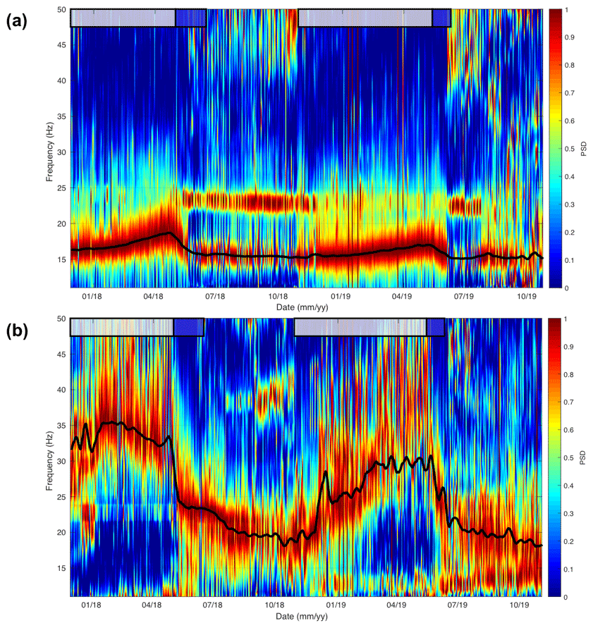
Figure 3 Normalized power spectra density (PSD) from hourly spectrograms of the passive seismic recordings of Laurichard site, from (a) C00 seismometer and (b) C05 seismometer. The bold black line denotes the moving-window average of hourly spectrogram maxima. Snow cover and melting periods are depicted by grey and blue boxes, respectively.

Among potential sources affecting the spectral content of seismic records, we aimed to select only natural resonance modes of the rock glacier structure. For example, we observed a very stable narrow peak of PSD at 23 Hz for both seismometers. This mode lights up mainly during summertime and in the daytime, although it remains visible during winter and in the nighttime but with significantly lower amplitude. Since this frequency peak is fully stable over time, we interpret its origin as either hydrological or anthropogenic. It may be generated by groundwater flow within the rock glacier (Roeoesli et al., 2016), by a pressure pipe located 400 m downstream or from road traffic coupled with a tunnel near Col du Lautaret (see Fig. 1). This frequency peak is also visible on spectrograms of station OGSA (see black arrow in Fig. 2d) located at Col du Lautaret at a stable site, suggesting a potential anthropogenic source. The spectral content of these recordings exhibits the same peak at 23–24 Hz (see red curve in Fig. 2d), implying it is not directly related to the rock glacier resonance. Thus this frequency peak is hereafter excluded from the analysis.

The spectral content of seismic recordings can be affected by temporal variations in ambient seismic noise sources. For the two sites, these sources are assumed to originate from stable human activities located in the nearby valley and from weathering, but they could also be partly related to hydrological processes via melting water in springtime and summertime. This source variability has to be addressed, in order to eliminate any spurious interpretation of actual changes in elastic properties. We then compare raw and normalized spectrograms of the reference station OGSA over 1 year (see Fig. C1 in Appendix C) to track any variation in the spectrum content which would prevent further comparison of frequency peaks observed on the rock glacier over time. No significant temporal changes in PSD appears within the illuminated spectrum of this stable station located near the Laurichard rock glacier. Another obvious fact to highlight is that frequencies which were picked from ambient noise are also often visible when earthquake signals are considered (see Appendix B). These two observations strengthen the direct link between these frequency peaks and rock glacier resonance.

Other spurious effects of artificial or non-specific sources affecting PSD are known: atmospheric effects (local structure or vegetation coupled with wind; Johnson et al., 2019), loss of sensor coupling or water filling of the shelter of the sensor during melt out (Carmichael, 2019). However, these sources are not present at the Laurichard rock glacier: for all sites the seismometers are well coupled on flat and stable boulders, ensuring a good rock-to-sensor coupling. Each of them is sheltered by a plastic tube covered by a waterproof tarp, in order to prevent any influence of rain, wind and snow. During site visits, no water in the settlement was observed.

For the C00 seismometer, we observe a main peak of PSD between 15 and 20 Hz interpreted as the fundamental mode of the nearby area of the rock glacier (Fig. 3a). The temporal evolution of this mode shows a seasonal cycle, characterized by higher frequencies during winters and lower frequencies during summers. A sudden drop of frequency occurs at the time when melting processes occur (blue boxes in Fig. 3). Comparing the two winter periods, the maximum frequency is lower in 2019 (about 17 Hz) than in 2018 (about 19 Hz), while it remains constant at approximately 15 Hz for the two recorded summers.

For sensor C05, we can follow the same peak that is considered the fundamental mode of the corresponding area, with a similar seasonal cycle (Fig. 3b). Again, the fundamental frequency increases during winter and drops during melting periods and summertime. Compared to the C00 case, the amplitude of this seasonal variation is much higher: even though the frequency value in summer is similar (about 15 Hz), the winter one reaches a higher value (about 30 Hz). The maximum value is also higher in 2018 (35 Hz) than in 2019 (30 Hz).

3.3 Resonance frequency monitoring of Gugla rock glacier

We applied the same spectral analysis for the Gugla site. From the hourly normalized PSD of seismic noise recorded on the rock glacier (sensor C2), we observed two resonance frequencies evolving with time (Fig. 4). At relatively high frequencies, a second mode is well measured, because the mean noise level is higher in Gugla than in Laurichard, where only the fundamental mode is observed.

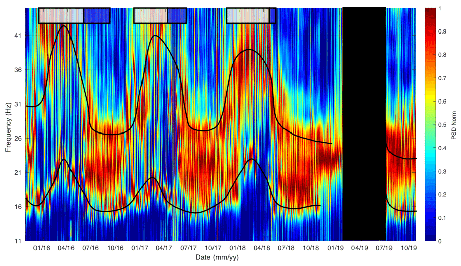
Figure 4 Normalized power spectral density (PSD) from hourly spectrograms of the ambient noise recordings of Gugla rock glacier, from C2 seismometer. Note the two bold black lines that roughly highlight the two spectral modes picked, for visibility purposes. Snow cover and melting periods are depicted by grey and blue boxes, respectively. No-data period is marked by a black box.

As for the Laurichard site, these frequencies present seasonal oscillations: they increase progressively to peak at cold winter periods, whereas they drop when melting processes occur in springtime and summertime (blue boxes in Fig. 4). The fundamental mode varies from 15 Hz in summertime to approximately 21 Hz in wintertime, whereas the second mode oscillates from 27 to 40 Hz.

Again, the resonance frequency of the fundamental mode shows an inter-annual variability: in winter 2017 the maximum value is lower (about 20 Hz) than the peaks of the two other winters (about 24 Hz).

4 Mechanical modeling

4.1 Methodology

Using a finite-element method, we model rock glaciers as vibrating structures embedded in the bedrock. We then study the sensitivity of the modal response of this model to ambient seismic noise as a function of its elastic properties.

Elastic features can be determined as a function of compressional V_p and shear V_s seismic wave velocities, together with the density ρ. Therefore we evaluate seismic velocities along depth thanks to active seismic investigations complemented by ground-penetrating radar (GPR) surveys in order to obtain a 1D $\left[V_{\mathrm{p}}\left(z\right),V_{\mathrm{s}}\left(z\right),\mathit{\rho }\left(z\right)\right]$ profile describing the medium near the seismometer of interest. This first model is considered a reference model since it has been built during unfrozen summer periods. In addition, we consider the effect of freezing–thawing processes on the elastic model using a poroelastic approach that enables us to quantitatively evaluate elastic parameter changes due to the freezing. Modal analysis is then performed with COMSOL software¹, in order to compute synthetic resonance frequencies that can be compared with the observed ones.

4.2 Reference model from geophysical investigations

For a few decades, numerous experiments have been devoted to the geophysical characterization of rock glaciers (Maurer and Hauck, 2007; Kneisel et al., 2008; Haeberli et al., 2010) in order to constrain site modeling and better understand subsurface physical processes involved in their deformation. Among available geophysical methods, seismic refraction tomography (SRT), ground-penetrating radar (GPR) and electrical resistivity tomography (ERT) have provided promising results. In Alpine permafrost regions, the high heterogeneity of the subsurface together with cost-intensive and risky field conditions makes geophysics challenging. However, combining the geophysical methods listed above gives useful information with respect to imaging and modeling the subsurface.

4.2.1 Laurichard rock glacier model

Ground-penetrating radar survey

We performed a ground-penetrating radar (GPR) campaign at the end of June 2019 to better assess the geometry and the internal structure of the Laurichard rock glacier. It is composed of (i) a common-offset longitudinal profile starting in the middle of the rock glacier and stopping near the front, following the main flow line, and (ii) a common-offset transversal profile crossing over the rock glacier width, approximately following the C01–C04 seismometer line discussed later (Fig. 1a). The method and resulting figures are shown in Appendix D.

Both GPR images show relatively continuous reflectivity within the rock glacier, particularly along the longitudinal direction (Fig. D1c), indicating a stratification of the deposits. A low-frequency antenna (25 MHz) certainly naturally homogenized the heterogeneity of rock glaciers, as witnessed by the quasi-absence of diffraction. The thickness of the glacier varies weakly along the longitudinal direction, ranging from 28 m upstream to 10 m downstream. More abrupt variations are detected in the transverse direction (Fig. D1d), from a few meters to 20 m at the center and the eastern part. It must be noted that the first few meters of the rock glacier cannot be resolved, due to the antenna configuration with a large source–receiver offset and the large wavelength (about 4.8 m).

As a conclusion, the bedrock interface depth is well constrained by GPR results, combining longitudinal and transversal profiles. In the lower part of the rock glacier near the front, the bedrock is estimated at an approximately 10 m depth. But the transversal profile also reveals heterogeneities over the seismic array. In the western part (C05) the rock glacier seems thinner than in the eastern part (C00), according to the bedrock depth estimation based on contour line interpolation on both sides of the rock glacier. By the digital elevation model (DEM) difference between surface and bedrock, we then more precisely estimated the interface depth (14 m for C00 and 8 m for C05; see Fig. 5b).

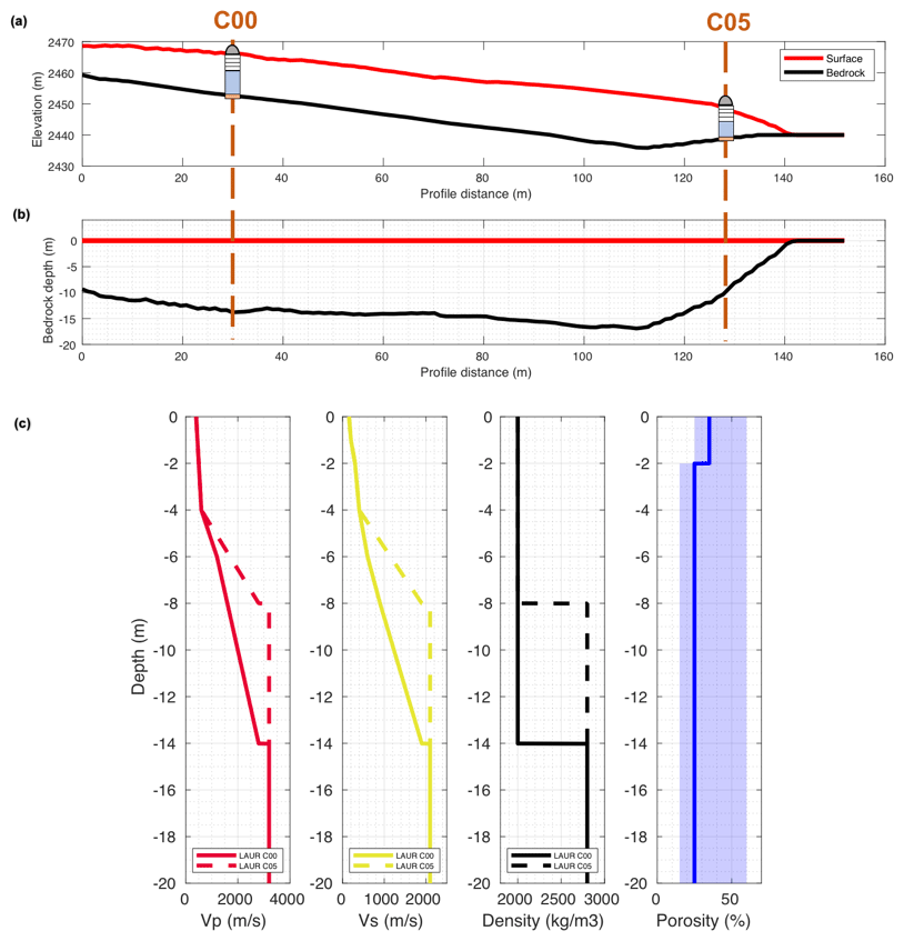
Figure 5 (a) Cross section of the Laurichard rock glacier digital elevation models (DEMs) of the surface and of the bed (taken for the bedrock) along the C05–C00 line. (b) The same profile, with the DEM of the surface as the reference. The vertical axis is then the bedrock depth starting from the surface. For both figures the location of the seismometers is indicated. (c) Seismic velocity models of the Laurichard rock glacier (continuous line for the C00 case, dashed line for the C05 case), based on geophysical investigations (seismic refraction) and the bedrock depth estimation, determined from DEM difference. The only difference between the two cases is the bedrock depth and consequently the seismic velocity gradient of the permafrost layer. In the two right panels the density and the medium porosity profile are shown (solid blue line), with low and high limits of the porosity used in the subsequent mechanical modeling.

Seismic tomography

A seismic refraction–tomography survey was performed in July 2019. This experiment consisted of active seismic recordings with controlled sources, in order to determine the P-wave velocity distribution along a 2D line. The profile is roughly located along the C1–C4 line, near the center of the seismic array (Fig. 1a). The method and resulting figure are shown in Appendix D and Fig. D2. The result shows 2D variations with some degree of layering in the velocity distribution. The interface between the rock glacier and the bedrock might be marked by the large interface separating a material with velocities lower than 2000 m/s with a layer showing a large velocity of about 3000 m/s (Fig. D2). Its thickness varies from 10 to 20 m, which is consistent with GPR results (Fig. D1c, d). To overcome the smoothing effect of seismic tomography, data have also been processed using seismic refraction with two opposite large-offset shots. This approach highlights a layered structure of the medium, with different slopes and particularly an interface located at around a depth of 4 m, which probably separates the active layer from the permafrost one. Therefore, we can assume an active layer from the surface to a 4 m depth, corresponding to the maximal depth where the medium is totally thawed in summertime.

Multichannel analysis of surface waves (MASW)

In order to better understand the seismic wavefield and constrain the S-wave velocity distribution at the site, we analyzed the surface Rayleigh waves, which dominate the vertical seismic records used in the tomography. The method and resulting figure are shown in Appendix D and Fig. D3.

The V_s profiles displayed in Fig. D3b show a large variability, but the best-fitting models all converge towards an interface located at a 5 m depth with a superficial velocity of 155 m/s followed by a linear increase in velocity reaching 750 m/s at a depth of 7 m. The best model also shows another deeper interface, at a 15 m depth, which could be the bedrock interface, despite the low resolution at this depth.

From all these geophysical surveys, a tentative 1D seismic velocity model was built for each seismometer (C00 and C05), as the reference unfrozen model. Its values have been well constrained by seismic refraction, whereas bedrock interface depth has been constrained by GPR results, together with interpolated DEM differences (Fig. 5).

4.2.2 Gugla rock glacier model

To establish a reference model of the Gugla rock glacier, we use seismic velocities that have already been constrained by a seismic refraction survey (Fig. 1b) performed in July 2017 during a summer and dry period (Fig. 6). All values for V_p and V_s profiles have already been presented in a previous study (Guillemot et al., 2020). We also assume a density profile that progressively increases, from ρ=2000 kg/m³ at the surface to ρ=2800 kg/m³ at the bedrock.

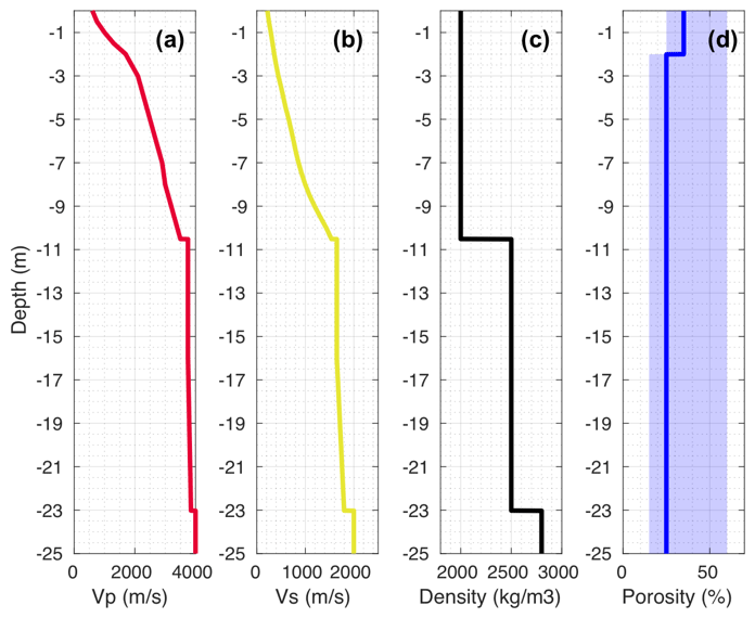
Figure 6 Seismic velocity models of the Gugla rock glacier, based on geophysical investigations (seismic refraction) and from borehole data, with P-wave velocity (a) and S-wave velocity (b) profiles. The density (c) and the medium porosity (d, solid blue line) profiles are also shown, with low and high limits of the porosity used in the subsequent mechanical modeling.

Moreover, we estimate the bedrock at a 23 m depth, in accordance with observations provided by boreholes located near the seismometer of interest (borehole F2; CREALP, 2015).

4.3 Freezing modeling from poroelastic approach

4.3.1 Methods and results

In order to mimic the freeze–thawing effect on resonance frequencies, the associated variations in elastic properties of the material have to be constrained by seismic velocity changes. A winter model is required for comparison to the summer one. For the transition from summer to winter, an increase in P- and S-wave velocities during winter is expected, in accordance with laboratory and numerical experiments (Timur, 1968; Carcione and Seriani, 1998; Carcione et al., 2010). Indeed, both bulk and shear moduli of the effective medium increase during freezing, generating a global stiffening of the upper part of the rock glacier subject to the seasonal thermal forcing.

In order to quantify the evolution of these elastic parameters with freezing, we use a poroelastic approach assuming a three-phase model: a rock glacier is considered a porous material composed of pores embedded into a granular rocky matrix. We then address the sensitivity of elastic parameters to the proportion of liquid water and ice filling the pores, for several porosity values. Since the wavelength of seismic waves is much greater than the size of the pores, this homogenization approach holds. As did Carcione and Seriani (1998), we use a Biot–Gassmann-type three-phase model that considers two solid matrices (rock and ice) and a fluid one (liquid water). Since the contribution of the air proportion within the pore is negligible on the shear modulus, which mostly determines the fundamental vibrating mode, we omit the air phase for the sake of simplicity.

We apply the following methodology for the three cases (Gugla C2, Laurichard C00 and Laurichard C05). Several parameters are required to completely describe the poroelastic state of a rock glacier: bulk and shear moduli of the respective pure phases, the averaged density, the porosity, and the water saturation.

For the summer state of the rock glacier, we evaluate these parameters indirectly. The density ρ is fixed at realistic values (ρ=1800 kg/m³ for the first 2 m; ρ=2000 kg/m³ for the deeper part of the rock glacier; and ρ=2650 kg/m³ for the bedrock; Hausmann et al., 2012), as well as the porosity profile (see references in Sect. 4.3.2). The water saturation s is assumed to be s=0 for the first 2 m, and s=0.2 when deeper, consistent with visual observations and qualitative features obtained from boreholes in summer (CREALP, 2016). Respective bulk and shear moduli of the pure phases (ice and water) are fixed from the example of Berea sandstone (Carcione and Seriani, 1998, Table 2). The bulk and shear moduli of the dry solid matrix have been obtained from the inversion of velocities using a Biot–Gassmann poroelastic model with two phases (solid matrix and water). For this inversion step, we use water saturation, porosity and seismic velocity profiles (V_p, V_s) deduced from seismic refraction geophysics performed in summer (see Fig. 5c for Laurichard and Fig. 6 for Gugla). The outputs of this inversion step are the elastic moduli of the solid matrix, assumed constant over seasons, and a description of the elastic behavior of the rock glacier with neither water saturation nor seasonal freezing. The profiles of all the parameters of this summer model are shown in Fig. 7b–e in red lines.

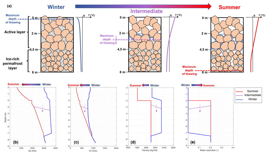
Figure 7 (a) Schematic cross section of the Gugla rock glacier in winter (left), in summer (right) and during the transition between them (intermediate state of thawing, middle), as well as a schematic temperature profile associated with each of them, showing the main assumptions of the freezing modeling methodology by a poroelastic approach described in the text. The porous medium is composed of a rock matrix (in orange) and pores filled by water (in blue) or ice (in grey). With respect to the maximum depth of thawing varying from the surface to the ZAA depth, the evolution of parameters used by the model is shown as follows: P-wave velocity (b), S-wave velocity (c), the averaged density (d) and the water saturation (d). The values in summer are obtained from geophysics and boreholes, whereas the values corresponding to a frozen state (pores fully filled by ice, no more liquid water) are obtained by the three-phase poroelastic model.

For the winter state of the rock glacier, we keep unchanged the porosity and elastic parameters of the three phases (water, ice and solid matrix), but we assume the pores are fully filled by ice (water saturation equals zero) from the surface to the maximum depth where seasonal freezing acts, also called the zero annual amplitude (ZAA) depth. ZAA is estimated to be approximately 8 m in depth from thermal investigations in Gugla (CREALP, 2016) and is extrapolated as well to Laurichard. The averaged density is computed by averaging the density of each phase, weighted by its respective volumetric ratio.

The seismic velocity profiles (V_p, V_s) for a totally frozen state are then computed by applying the three-phase poroelastic model. For this step, the input parameters are the porosity and the density, together with bulk and shear moduli of each phase (water, ice and solid matrix). These elastic parameters are homogenized according to Carcione and Seriani (1998), and then equations of wave propagation are solved in order to obtain fast P-wave and S-wave velocities as modeled by Leclaire et al. (1994). Results of the evolution of these velocities with respect to the ice ∕ water ratio filling the pores are shown in Fig. 8 for the example of Laurichard (sensor C00). Hence we deduce the values for a frozen state of the rock glacier with pores totally filled by ice between the surface and ZAA. We acknowledge that this is a strong assumption for the winter state and that other models may also explain our observations. The profiles of all the parameters of this winter model are shown in Fig. 7b–e with blue lines.

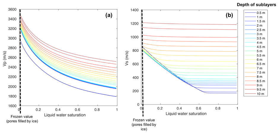
Figure 8 (a) Evolution of P-wave velocity V_p with respect to the ratio between water and ice filling the pores, resulting from the Biot–Gassmann-type three-phase poroelastic model, applied to the Laurichard rock glacier (for C00 seismometer). The different curves correspond to the different sublayers, whose depth is indicated in the right panel. The V_p values used to model the winter state are those for liquid water saturation tending towards zero. (b) Same results for S-wave velocity V_s.

With these two models in summer (minimum of freezing) and winter (maximum of freezing), we can also model the transition between them. Although the freezing process (from summer to winter) is poorly constrained, due to liquid water infiltration and complex thermal forcing, the thawing process (from winter to summer) appears easier to model, assuming a temporal evolution of thawing mainly controlled by thermal heat waves propagating from the surface to the ZAA depth. Hence, we build an intermediate state of the rock glacier by introducing another parameter, called “maximum depth of thawing” (see Fig. 7a). This parameter establishes an interface between the unfrozen state (as the summer model) above it and the frozen state (total pore filling by ice) below it. Hence, this maximum depth of thawing evolves from the surface to the ZAA with 1 m increments, reporting as many intermediate models. The profiles of the parameters of an example of an intermediate model are shown in Fig. 7b–e in dashed purple lines.

Finally, we compute the modal response (explained below in Sect. 4.4) of the corresponding vibrating structure of all these models (summer, intermediate and winter), modeling a value of resonance frequency depending of the freezing state of the rock glacier.

4.3.2 Influence of the porosity

Defined as the ratio between pore volume and total volume, the porosity ϕ of the rock glacier is one of the key parameters influencing the mechanical modeling. Our three-phase poroelastic model actually considers the filling of pores by two phases (ice and water), together with interaction between ice and rocky debris matrices that strongly depends on porosity. In the absence of any in situ information, we assume a model of spherical-particle stacking (Rice, 1993), decreasing with depth due to compaction (ϕ=0.35 for sublayers from the surface to a 2 m depth and ϕ=0.25 elsewhere below, for both sites). In order to quantitatively assess the sensitivity of our results to porosity, we also apply the mechanical modeling to other profiles considering extreme values (low limit ϕ=0.2 in the active layer and ϕ=0.15 elsewhere and high limit ϕ=0.6 everywhere for this rock glacier lithology (Arenson and Springman, 2005)). As expected, the higher the porosity values, the higher the influence of the ice pore filling on the elastic parameters and thus the higher the variation in modeled resonance frequencies. In the following results presented below, error bars correspond to the sensitivity to the porosity (low limit for low porosity, high limit for high porosity; see values in transparent shading in Fig. 10).

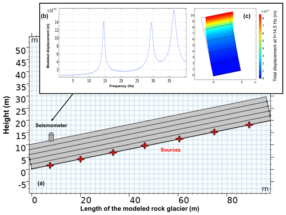
Figure 9 (a) First 2D model of the terminal part of Laurichard rock glacier, with realistic longitudinal dimension (length) and location of synthetic seismic sources and seismometer. (b) Output of the frequency response function (FRF) of this model, as the vertical displacement recorded by the seismometer along frequencies. Peaks of this curve indicate resonance frequencies of modes of the modeled structure with a vertical component. (c) The 2D rock glacier model with reduced longitudinal dimension (5 m) and with symmetrical conditions at boundaries perpendicular to the slope. Since the FRF of this model shows the same peaks as the first one, this reduced model is only used for the modal analysis for the sake of simplicity.

Figure 10 Results of the modal analysis for Gugla (GUGL) and Laurichard (LAUR) rock glaciers. The evolution of the resonance frequency of the respective synthetic modes is plotted, according to the maximal depth of thawing from the surface to the ZAA (8 m depth): left stands for the state of maximal freezing in winter (frozen medium until 8 m depth) and right for the summer (unfrozen medium). The range of measured resonance frequency values is shown by the squares in the corresponding colors (estimated from Figs. 3 and 4 for respective sites). Error bars (in transparent shading) show the influence of porosity on the results: the low (high) limit of error bars shows the results for extremely low (extremely high) porosity profile.

4.4 Modal analysis and frequency response of the rock glacier

We build a mechanical model in COMSOL software based on the finite-element method, in order to numerically compute its resonance frequencies and modal response (see Appendix E for details). The rock glacier is modeled as a 2D rectangular vibrating structure embedded in the bedrock (or a stable bottom layer). The height H of the structure is fixed at the corresponding depth of bedrock (see Fig. 5 for Laurichard and Fig. 6 for Gugla). The model is vertically sub-sampled into 2 m thick sublayers, with elastic parameters interpolated from averaged values of seismic tomography results and with a usual isotropic attenuation factor of 1 % (Bonnefoy-Claudet et al., 2006). Depending on the direction of the model (longitudinal or transversal), the width of the structure varies in accordance with the whole rock glacier size (several tens of meters), permitting an infinity of vibration modes. Based on a polarization analysis from ambient noise between 1 and 50 Hz in the Gugla rock glacier in summer 2016, we observed that the wavefield of rock glaciers is mostly polarized in a parallel to the slope direction. Similar to the fundamental mode of an unstable rock mass (Burjánek et al., 2012) and avalanche glaciers (Preiswerk et al., 2019), the measured polarization is almost linear (ellipticity lower than 0.15) and thus corresponds best to shear modes. We then computed the frequency response function (FRF) (Fu and He, 2001) on the whole length (several hundreds of meters for both cases) of the rock glacier, in order to obtain its resonance frequencies corresponding to vibration modes of the mechanical structure. For this step, we simulated several seismic sources located at the base of the vibrating structure (see red crosses in Fig. 9a), producing harmonic forces from 1 to 50 Hz in all directions. The amplitude of this modeled seismic noise is not frequency-dependent, while it decreases generally with frequency in the field, probably showing the excitation of modes other than the recorded ones (especially in Laurichard). However, after checking that resonance frequencies obtained from the FRF with a high amplitude of vertical displacement (Fig. 9b) would not be modified, we reduced the width of the model to 5 m by applying symmetrical conditions at the boundaries perpendicular to the slope (Fig. 9c), in order to facilitate the following parametric modal analysis.

4.5 Comparison between observed and modeled resonance frequencies

We show the results from the modal analysis in COMSOL software for only the observed modes with a vertical component (first mode for Laurichard, the first two modes for Gugla) in Fig. 10. Nine mechanical models have been tested, corresponding to different steps of thawing with elastic parameters selected as described in Sect. 4.3. Thus, we present modeled resonance frequencies with respect to the maximal depth of thawing, from the surface to an 8 m depth (Fig. 10). As expected, resonance frequencies of these modes match the frequency band of measurements below 50 Hz and generally decrease with thawing. We compare them to the maximum (in winter) and minimum (in summer) values observed at all sites (depicted in squares in Fig. 10, which are values from Fig. 3 for Laurichard and Fig. 4 for Gugla). The modeled resonance frequencies fit well the observed ones, considering error bars related to porosity uncertainties (see Sect. 4.3.2). Regarding the fundamental mode (mode 0), the resonance frequency is of the same order of magnitude (between 15 and 20 Hz) for both sites (i.e., Gugla and Laurichard). Focusing on the two sensor locations in Laurichard, a stronger effect of freezing is observed for C05 than for the C00 model. Hence, the bedrock is shallower under C05 than under C00 (8 and 14 m, respectively), highlighting the role of the height of the local vibrating structure on seasonal amplitudes. In general, these numerical results explain well the seasonal variations in observed resonance frequencies, assuming a thawing process from the surface to an 8 m depth between winter and summer.

5 Discussion

From the results of mechanical simulation on both the Laurichard and the Gugla rock glaciers, we draw several conclusions:

• The vibrating modes of rock glaciers can be tracked from spectrograms of seismic ambient noise. The resonance frequencies from the mechanical modeling fit well the measured ones (between 15 and 20 Hz in summer for both sites) within experimental error bars. This validates our methodology based on rock glacier modeling as a vibrating structure, at least for the first mode.

• Monitoring these resonance frequencies over time allows us to observe seasonal evolution – all the modes show a progressive increase in the resonance frequencies during winter, followed by a sudden drop at the onset of melting periods in spring and lower values during summers.

• According to the poroelastic approach used to model the effect of freezing on seismic velocities, this variation is qualitatively well explained by freeze–thawing processes. Indeed, the annual heat wave propagates into the surface layers of the rock glacier (Cicoira et al., 2019; CREALP, 2016), causing a change in frozen material content within the porous medium and thus a large variation in elastic properties due to this thermo-mechanical forcing. For both sites and sensor locations, this modeled mechanical forcing provides a good estimation of the observed frequencies' seasonal variations, quantitatively. The modeled changes in elastic parameters (bulk and shear moduli increasing through seismic velocities) involved for the Gugla rock glacier (Guillemot et al., 2020) have thus been improved by this complementary method based on a more complete description of poroelasticity, though other models may also explain our observations.

• By tracking resonance frequencies in the long term, we are able to detect an inter-annual variability. Interestingly, the freezing process appears to correlate with an annual minimum of resonance frequency – as an example, in 2019 in Laurichard, the winter resonance frequency was lower than in 2018, indicating a lower rigidity of the medium due to reduced frozen material content. The winter was actually colder in 2018 than in 2019 – from a meteorological station near Col du Lautaret (1 km from Laurichard), the mean air temperature during snow cover T_winter was lower in 2018 ($T_{\mathrm{winter}}\left(\mathrm{2018}\right)=-\mathrm{2.07}$ ^∘C) than in 2019 ($T_{\mathrm{winter}}\left(\mathrm{2019}\right)=-\mathrm{0.50}$ ^∘C). The intensity of freezing is generally estimated from freezing degree days (FDDs), defined as a time cumulative sum of each ground surface temperature below 0 ^∘C recorded during one wintertime. The snow cover period, which insulates the ground from air forcing, was earlier and longer in 2019 than in 2018, and so the internal freezing of the rock glacier was less intense in 2019 (FFD $\left(\mathrm{2019}\right)=-\mathrm{322}$ ^∘C d) than in 2018 FFD $\left(\mathrm{2018}\right)=-\mathrm{451}$ ^∘C d). Similarly for the Gugla site, the winter resonance frequency was significantly lower in 2017 (19 Hz) than in the others years (about 23 Hz). Despite a comparable mean air temperature between 2016 and 2017, the earlier and longer snow cover period in 2017 promoted a lower freezing of the internal layers. We finally conclude that resonance frequency in wintertime indicates well the intensity of freeze–thawing effects on the rock glacier.

• Despite a high level of heterogeneities within rock glaciers, low-frequency GPR results allow us to better constrain the bedrock interface depth. For Laurichard, the mean value was estimated at 10 m (±50 % due to the slope underneath). According to field observations and DEM interpolation, we fixed this value at 14 m for the C00 model and 8 m for the C05 model. This unique difference between the two locations explains very well the observed difference in seasonal resonance frequency amplitude (Fig. 3) – the shallower the bedrock interface, the larger this amplitude. In addition to active seismology allowing us to perform 2D seismic velocity tomographies, low-frequency GPR results provide valuable information about internal structure of the surveyed rock glaciers, reinforcing the benefits of geophysical investigations in combination with passive seismology in rock glaciers.

The relation between ground surface temperature and resonance frequencies is plotted in Fig. 11 (for Laurichard C00 case). It reveals an annually repeated pattern showing a hysteretic behavior. This relation suggests several phases throughout the year (indicated with colors and numbers in Fig. 11b), depending on the state of freezing of the rock glacier: (1) unfrozen phase (late summer and autumn), when temperature is varying above 0 ^∘C while resonance frequency stays at its lowest level; (2) shallow freezing phase (late autumn and early winter), when temperature decreases to below 0 ^∘C (with possible significant drops depending on the presence of snow cover insulating the medium or not), while resonance frequency starts to increase; (3) deep freezing phase (late winter), when temperature is stabilized due to insulation by permanent snow cover, while the freezing front propagates deeper, increasing the resonance frequency; (4) shallow thawing phase (early spring), when temperature reaches 0 ^∘C and stays constant during a zero-curtain period, indicating phase change together with melting water percolating into the active layer and sometimes re-freezing, while resonance frequency drops due to thawing of surface layers; and (5) deep thawing phase (late spring and early summer), when the heat wave propagates deeper in the medium, keeping the decrease in resonance frequency up.

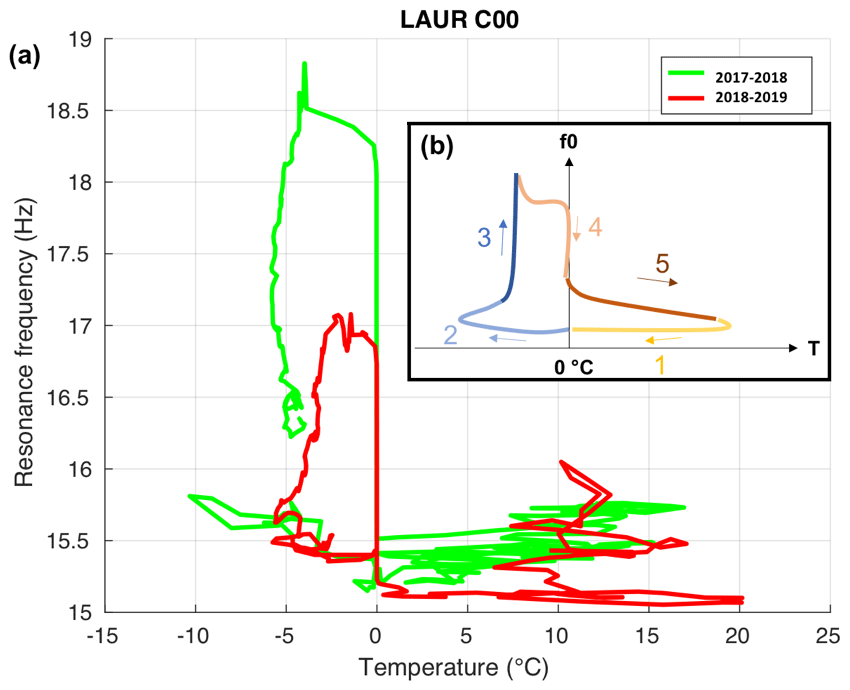
Figure 11 (a) Diagram of daily averaged ground temperature (recorded by miniature temperature data loggers) versus daily averaged resonance frequency of the first mode recorded by C00 seismometer at Laurichard rock glacier. The green line corresponds to data from December 2017 to November 2018, while the red line corresponds to data from December 2018 to October 2019. (b) Schematic generalization of the ground surface temperature dependency of resonance frequency on freezing–thawing cycle, showing an hysteretic loop composed of five phases described in the text.

Figure 12 Example of (normalized) depth sensitivity kernels of the two passive seismic methods for the Laurichard (C00 seismometer) rock glacier model. The red curve corresponds to the modal analysis (resonance frequency of the first vibrating mode). The other curves correspond to the ambient noise correlation (relative change in the Rayleigh wave velocity dV∕V, depending on the frequency, shown by the other colors). At high frequencies (> 14 Hz), dV∕V is most sensitive at shallower depths than the resonance frequency of the first mode, whereas at low frequencies (< 14 Hz), dV∕V is most sensitive at deeper depths than resonance frequency.

In comparison with other passive seismic methods, such as relative seismic velocity variations computed from ambient noise correlation that have already been applied in Gugla (Guillemot et al., 2020), the spectral analysis of seismic noise (presented here) is easier to process. Combined with the modal analysis of a mechanical model of the site, the spectral content accurately records the seasonal freeze–thawing cycle, reinforcing observations from ambient noise correlation (Guillemot et al., 2020). Beyond these similarities, the main difference between these two methods is their depth sensitivity. Frequency resonance focuses on isolated frequencies, whereas ambient noise correlations exploit the whole spectrum, thereby surveying a larger range of depths. To quantify this difference between the two methods, we computed sensitivity kernels for each one. This consists in evaluating the changes (of frequency or dV∕V) after a 50 % increase in seismic velocities V_p and V_s for a 0.5 m thick sublayer along the depth of the modeled rock glacier. All the parameters are those of the summer models (for Gugla in Fig. 6, for Laurichard C00 and Laurichard C05 in Fig. 5c), and kernels have been computed for all these three sites. These results are presented in Fig. 12. (1) For the ambient noise correlation method, we compute the dispersion curves of the Rayleigh waves using the Geopsy package (Wathelet et al., 2004). The theoretical relative velocity changes (dV∕V) are computed by measuring the difference between the modified dispersion curve and the reference one at each frequency. (2) For the modal analysis method, the resonance frequency of the fundamental mode of the vibrating structure modeling the rock glacier is obtained using COMSOL software. For both methods, their kernels have been normalized by their maximum value along the depth, allowing for an estimation of the depth where the sensitivity of the method is the highest. The results are shown in Fig. 12 for the Laurichard C00 sensor, while other sites are not presented but yield similar results. For all sites, modal analysis is most sensitive at a relatively shallow depth (5 m for Gugla, 4 m for Laurichard C00, 3 m for Laurichard C05) in the active layer, whereas ambient noise correlation has a broader sensitivity, including shallower and deeper layers depending on the frequency band (the lower the frequency, the deeper the penetration). Therefore, the modal analysis permits us to easily evaluate the state of freezing of rock glaciers, surveying mostly the depth range between 2 and 8 m, including the active layer (< 5 m), while ambient noise correlation at low frequencies allows the same monitoring over a broader range of depths but requires additional data processing. Furthermore, ambient noise correlation may provide less stable results at high frequencies (up to 14 Hz, for the Gugla study; Guillemot et al., 2020), preventing any interpretation of the chaotic results due to the lack of high-frequency noise in the cross-correlation at a large inter-sensor distance. Hence, the sensitivity of the different methods depends also on the nature of the ambient noise wavefield together with the sensor network setup. According to the site and its instrumentation, the two passive seismic methods may be combined to obtain stable results along the whole depth of the rock glacier. As with many other geophysical techniques, the present study is therefore to be considered one element among other parts of a global monitoring strategy.

6 Conclusions

For two rock glaciers, we monitored the resonance frequencies of vibrating modes over several years thanks to continuous seismic noise measurements. These frequencies show seasonal variations, related to changes in elastic properties of the structure underneath the recording sensor, due to freeze–thawing effects. Assuming vibrating systems, we performed a 2D mechanical modeling of rock glaciers, which fits well the recorded resonance frequencies. By estimating elastic properties derived from active seismic measurements, we have reproduced the observed lowest values in summer, when the active layer is totally thawed. By quantitatively modeling the increase in rigidity due to freezing in wintertime using a poroelastic approach, we have reproduced the observed higher values in winter due to maximum freezing in the active layer. These results highlight the sensitivity of resonance frequency to seasonal freeze–thawing cycles.

The results of this modal analysis have been obtained from a model constrained by geophysical investigations, such as ground-penetrating radar and seismic tomography surveys. This study shows that the two approaches (spectral analysis of seismic data, combined with GPR and seismic refraction) provide a consistent understanding of seasonal variations in rock glacier rigidity, mainly forced by the freezing effect of those porous media.

Among passive seismic methods applied to rock glaciers, the spectral analysis appears to be an easy and effective monitoring tool of the active layer, which is subjected to significant seasonal changes. At greater depths and lower frequencies, the seismic data are preferably processed using a pair of stations by computing ambient noise correlation. This can be useful to complement observations of resonance frequencies, in addition to bringing new insights into other processes occurring at greater depths, such as groundwater or structural changes within rock glaciers. In the long term, seismic vibrations offer the possibility of monitoring the effect of global warming on permafrost degradation.

Appendix A: Time series of ground surface temperature (Laurichard rock glacier)

In Fig. A1 we show the time series of the measured ground surface temperature at several locations on and near the Laurichard rock glacier. These measurements help to date the snow cover periods with a zero-curtain effect, together with freezing periods.

Figure A1 (a) Location of the five miniature temperature data loggers (MTDs) that record the temperature of the subsurface (below 2–10 cm of debris) every hour, shown in (b) over the first 2 years of data, with snow cover (grey boxes, when temperature is below 0 ^∘C) and melting (blue boxes, when zero-curtain effect occurs) periods highlighted.

Appendix B: Frequency picking of earthquake signals

In addition to spectral analysis from ambient noise, PSDs of earthquake signals emerging from noise have also been computed. For both sites, such signals have been sorted out from a catalog of earthquakes (magnitude M>2). For the Laurichard area, we used all earthquakes recorded by the Sismalp catalog (https://sismalp.osug.fr/evenements, last access: 29 January 2021). We thus applied the same processing as for noise (without any clipping) for the 60 s long raw trace containing the signal of earthquakes and finally tracked resonance frequencies of these quakes by maxima picking (Fig. 2). For the Laurichard site, we used seismic traces of another station located in a stable area at Col du Lautaret (see Fig. 1), named OGSA (RESIF, 1995). Since OGSA is considered a reference station, we computed site-to-reference spectral content to evaluate the specific frequency peaks of the Laurichard rock glacier (see Fig. B1). In this way, we ensured that those frequencies picked were related to the modal signature of the rock glacier. Overall, this method of spectral analysis allows for comparing the spectral response of the structure to low (seismic noise) and higher (earthquakes) levels of excitation.

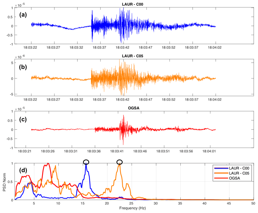
Figure B1 Seismic signals of an earthquake (vertical ground velocity in m/s) recorded by sensors C00 (a) and C05 (b) at Laurichard rock glacier and by OGSA station at Col du Lautaret (c), 29 June 2018 at 18:00 UTC. (d) The normalized PSD of the respective signals. Black circles highlight the maxima of these spectrograms that have been picked by using our method (details in the text). The same method has been used for ambient noise recordings.

The resonance frequencies estimated using earthquake signals (white dots in Fig. B2) appear similar to the ones estimated from noise for the C00 seismometer. However, there are more discrepancies for sensor C05. For this sensor, the peak frequencies determined from seismic signals show more fluctuations than when picking resonance frequencies from the PSD of seismic noise.

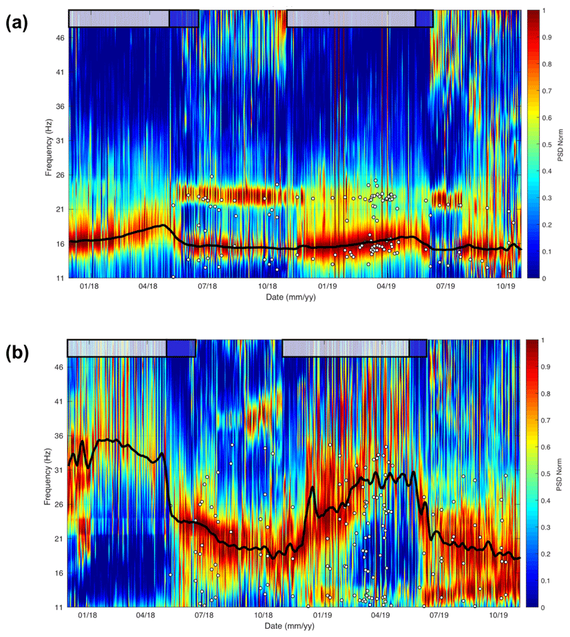
Figure B2 Normalized power spectral density (PSD) from hourly spectrograms of the passive seismic recordings of Laurichard site from (a) C00 seismometer and (b) C05 seismometer. The bold black line denotes the moving-window average of hourly spectrogram maxima. For each recorded earthquake (M>2), the local maxima have been automatically picked (white dots) if they appear significantly on the spectrogram. Snow cover and melting periods are depicted by white and blue boxes, respectively.

Appendix C: Ambient noise source variability over 1 year

In order to address the effects of seasonal changes in seismic sources, we compare raw and normalized spectrograms of seismic recordings acquired both on rock glaciers and on a stable nearby site. Here we present the results for the OGSA station (RESIF, 1995), located at Col du Lautaret (2 km from the Laurichard rock glacier) in 2019 (see Fig. C1). From these raw spectrograms, we observe a seasonal variability in the noise level, suggesting a seasonal variability in the noise sources (higher in summer than in winter, probably due to intensified road traffic and fluvial processes in summer). From the normalized spectrograms, we notice that no significant changes in frequency peaks appear within the illuminated spectrum of interest (10–40 Hz). Since the OGSA station (stable reference) is located close to the Laurichard rock glacier, we assume that ambient noise sources are roughly the same for both sites. Therefore we conclude that seasonal variability in frequency peaks recorded on the rock glacier between 15 and 40 Hz (see Fig. 3) is not much influenced by seismic source changes but rather linked to the specific resonance of the rock glacier structure.

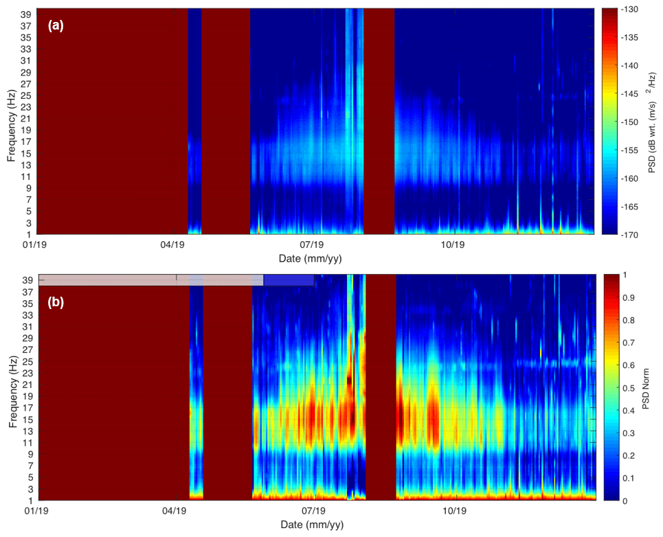
Figure C1 Daily raw (a) and normalized (b) spectrograms of power spectral density (PSD) from OGSA station, located at 2 km from the Laurichard rock glacier, in a stable site, for all of the year 2019.

Appendix D: Geophysical surveys in Laurichard rock glacier

D1 Ground-penetrating radar survey

Preliminary tests have demonstrated the ability of the 25 MHz rough-terrain antennas (RTAs) to follow the continuity of the reflectors throughout the glacier, despite a lower resolution (wavelength about 4.8 m). The 100 MHz antennas actually experienced penetration problems, presumably related to the presence of heterogeneities equivalent in size to the wavelength (about 1.2 m). In addition, a common-middle-point (CMP) survey was performed along the western part of the transverse profile using unshielded bi-static 100 MHz antennas, in order to assess locally the electromagnetic wave velocity distribution within the glacier. Figure D1a shows the CMP data after trace-by-trace amplitude normalization and gain amplification using a dynamic automatic gain control computed in a 100 ns time window. After the direct air and ground waves, numerous events exhibiting a hyperbola shape can be recognized from 40 to 225 ns in the CMP data. These hyperbolas have been analyzed considering a semblance analysis (Fig. D1b), which yields the stacking velocity versus propagation time where a semblance is maximal. The picked maximum of the velocity distribution shows variations ranging from 14 to 11 cm/ns with a mean velocity of 12 cm/ns. As these variations are measured on apparent velocities, the real variations are larger when layers are considered. They can be qualitatively interpreted in terms of an increase in air (velocity of 30 cm/ns) and ice (velocity of 17 cm/ns) content when velocity is large and an increase in water content (velocity of 3.33 cm/ns) when velocity drops. Considering a mean velocity of 12 cm/ns, the 100 MHz CMP analysis penetrates to a depth of 13.5 m and the increase in velocity located close to 110 ns corresponds to a depth of around 6 m.

Figure D1c and d show both common-offset profiles acquired using the 25 MHz antennas after they were processed using (i) time-zero source correction, (ii) normal-moveout correction as source and receivers are separated by an offset of 6.2 m for these antennas, (iii) static corrections for topography, (iv) migration, and (v) time-to-depth conversion. The later processing steps have been performed considering a mean velocity of 12 cm/ns, a value deduced from the CMP analysis (Fig. D1b).

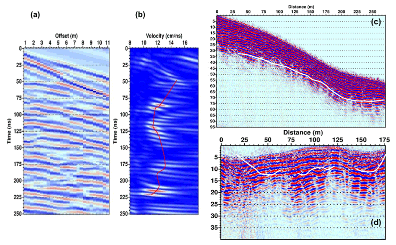
Figure D1 GPR results for Laurichard rock glacier, with (a) common-middle-point GPR data acquired with a 100 MHz unshielded antenna. (b) Velocity analysis displaying the semblance according to apparent velocity and propagation time. The red curve indicates the picked maximum of semblance. (c) Common-offset 25 MHz longitudinal profile. Elevation corrections have been divided by a factor of 2 for visibility purposes. (d) Common-offset 25 MHz transverse profile. For (c) and (d), the vertical / horizontal ratio axis has been scaled by a factor of 2.4 and the bedrock interface is highlighted by a white curve.

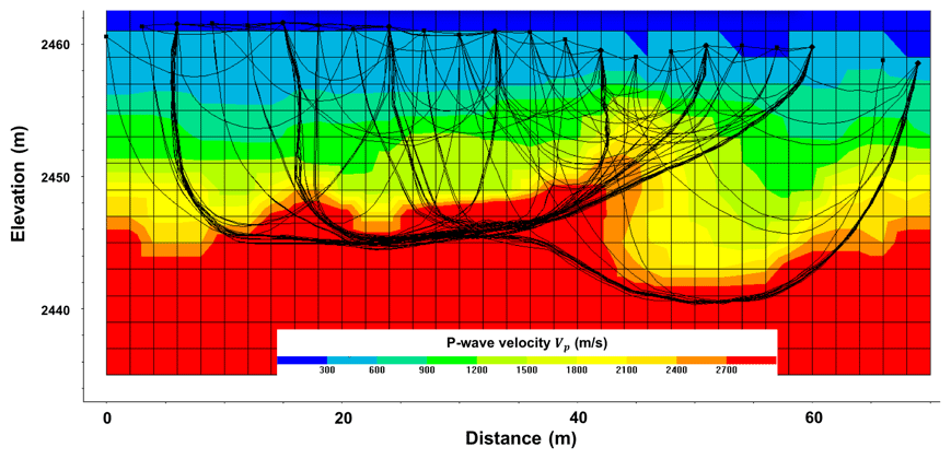
Figure D2 P-wave velocity distribution of Laurichard rock glacier, obtained from seismic tomography data acquired along the transversal profile of seismic refraction (yellow circles in Fig. 1d) in summertime. The different ray paths are shown with black curves. The seismic velocities were used to constrain bedrock depth and P-wave velocity profiles for the mechanical modeling.

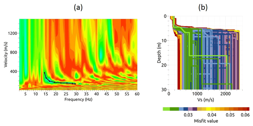
Figure D3 Multichannel analysis of Rayleigh waves propagating within the rock glacier. (a) Semblance velocity–frequency map highlighting several modes, the fundamental dispersion curve being picked as indicated by the black line, and (b) V_s distribution versus depth derived from the inversion of the fundamental dispersion curve. Colors indicate the RMSE (color bar in %) between synthetic and picked fundamental dispersion curves (best-fitting model in green).

D2 Seismic tomography

A seismic refraction–tomography survey was performed in July 2019. This experiment consisted of active seismic recordings with controlled sources, in order to determine the P-wave velocity distribution along a 2D line. The profile composed of 24 geophones (4.5 Hz) deployed every 3 m was roughly located along the C1–C4 line, near the center of the seismic array (Fig. 1a). The first arrival time picking of the eight shots were inverted using a simultaneous iterative reconstruction technique (SIRT; Demanet, 2000) in order to obtain the P-wave velocity distribution along the profile (Fig. D2). From an initial model with a uniform velocity of 3000 m/s (340 m/s in the air), 25 iterations were performed to reconstruct observations (RMSE =8 ms).

D3 Multichannel analysis of surface waves (MASW)

In order to better understand the seismic wavefield and constrain the S-wave velocity distribution at the site, we analyzed the surface Rayleigh waves, which dominate the vertical seismic records used in the tomography. For this, we used a far-offset shot and computed the semblance map of the velocity and frequency of the waves dominating the seismic record (Fig. D3a), obtained using the Geopsy package (Wathelet et al., 2004).

The semblance map shows several continuous modes, while the fundamental dispersion curve was picked from 14 to 30 Hz, as indicated by the black line. The presence of several other modes is due to the presence of strong contrasts within the rock glacier and at the interface between the rock glacier and the bedrock. The dispersion curve was inverted using the Geopsy dinver package (Wathelet et al., 2004), where a global-neighborhood-algorithm optimization method is implemented. The model was parametrized using four layers, the top three searching for linear velocity gradients in each layer. With the available frequency range and the velocity distribution, the resolution at large depths (> 15 m) is rather poor.

Appendix E: Modal analysis using finite-element method

The finite-element method aims to numerically estimate the resonance frequencies of a vibrating structure, by solving Newton's second law for the displacement of the considered degrees of freedom V(t) (Bathe, 2006). Assuming free-equilibrium and no attenuation, the equation is

$$\begin{array}{}\text{(E1)}& \left[\mathbf{M}\right]\left\{\ddot{V}\left(t\right)\right\}+\left[\mathbf{K}\right]\left\{V\left(t\right)\right\}=\left\{\mathrm{0}\right\},\end{array}$$

where [M] is the global mass matrix, [K] is the global stiffness matrix and the dots mean the time derivative. Both [M] and [K] matrices are obtained by correctly assembling the respective element matrices, in accordance with the finite-element method (Bathe, 2006).

As a result, the solutions of Eq. (E1) have to be of the form

$$\begin{array}{}\text{(E2)}& \left\{V\left(t\right)\right\}=\left\{\mathit{\psi }\right\}\sin \left[\mathit{\omega }\left(t-t_{\mathrm{0}}\right)\right],\end{array}$$

where {ψ} refers to a vector of order n, ω is a constant identified to the corresponding pulsation of the vibrating mode {ψ}, and t and t₀ are the time variable and an arbitrary time constant, respectively.

Equations (E1) and (E2) provide the generalized eigenproblem:

$$\begin{array}{}\text{(E3)}& \left[M^{-\mathrm{1}}K\right]\left\{{\mathit{\psi }}_j\right\}={\mathit{\omega }}_j^{\mathrm{2}}\left\{{\mathit{\psi }}_j\right\}.\end{array}$$

By solving this linear system, we can deduce the modal parameters: the n eigenvalues ${\mathit{\omega }}_j^{\mathrm{2}}$ (with $\mathrm{0}\le {\mathit{\omega }}_{\mathrm{1}}^{\mathrm{2}}\le {\mathit{\omega }}_{\mathrm{2}}^{\mathrm{2}}\le \mathrm{\dots }\le {\mathit{\omega }}_n^{\mathrm{2}}$) and the corresponding eigenvectors {ψ_j}. The eigenvector {ψ_j} is called the jth modal shape vector that vibrates at the frequency $f_j={\mathit{\omega }}_j/\left(\mathrm{2}\mathit{\pi }\right)$.