A seasonal algorithm of the snow-covered area fraction for mountainous terrain

The snow cover spatial variability in mountainous terrain changes considerably over the course of a snow season. In this context, fractional snow-covered area (fSCA) is an essential model parameter characterizing how much ground surface in a grid cell is currently covered by snow. We present a seasonal fSCA algorithm using a recent scale-independent fSCA parameterization. For the seasonal implementation, we track snow depth (HS) and snow water equivalent (SWE) and account for several alternating accumulation–ablation phases. Besides tracking HS and SWE, the seasonal fSCA algorithm only requires subgrid terrain parameters from a fine-scale summer digital elevation model. We implemented the new algorithm in a multilayer energy balance snow cover model. To evaluate the spatiotemporal changes in modeled fSCA, we compiled three independent fSCA data sets derived from airborne-acquired fine-scale HS data and from satellite and terrestrial imagery. Overall, modeled daily 1 km fSCA values had normalized root mean square errors of 7 %, 12 % and 21 % for the three data sets, and some seasonal trends were identified. Comparing our algorithm performances to the performances of the CLM5.0 fSCA algorithm implemented in the multilayer snow cover model demonstrated that our full seasonal fSCA algorithm better represented seasonal trends. Overall, the results suggest that our seasonal fSCA algorithm can be applied in other geographic regions by any snow model application.

1 Introduction

In mountainous terrain, the large spatial variability in the snow cover is driven by the interaction of meteorological variables with the underlying topography. Over the course of a winter season, the dominating topographic interactions with wind, precipitation and radiation vary considerably, generating characteristic seasonal dynamics of spatial snow depth variability (e.g., Luce et al., 1999). This spatial variability, or how much of the ground is actually covered by snow, is typically characterized by the fractional snow-covered area (fSCA). The fSCA is a crucial parameter in model applications such as weather forecasts (e.g., Douville et al., 1995; Doms et al., 2011), hydrological modeling (e.g., Luce et al., 1999; Thirel et al., 2013; Magnusson et al., 2014; Griessinger et al., 2016, 2019) and avalanche forecasting (Bellaire and Jamieson, 2013; Horton and Jamieson, 2016; Vionnet et al., 2014), and it is also used for climate scenarios (e.g., Roesch et al., 2001; Mudryk et al., 2020).

The fSCA can be retrieved from various satellite sensor images, including Moderate Resolution Imaging Spectroradiometer (MODIS) or Sentinel-2 (e.g., Hall et al., 1995; Painter et al., 2009; Drusch et al., 2012; Masson et al., 2018; Gascoin et al., 2019). Nevertheless, solutions are required to correct for temporally and spatially inconsistent coverage due to time gaps between satellite revisits, data delivery and the frequent presence of clouds (Parajka and Blöschl, 2006; Gascoin et al., 2015). Though fine-scale spatial snow cover models provide spatial snow depth distributions that could be used to derive coarse-scale fSCA, applying such models to larger regions is generally not feasible. This is in part due to computational cost, a lack of detailed input data and limitations in model structure or parameters. While some of these limitations can be overcome using current snow cover model advances applying data assimilation routines (e.g., Andreadis and Lettenmaier, 2006; Nagler et al., 2008; Thirel et al., 2013; Griessinger et al., 2016; Huang et al., 2017; Baba et al., 2018; Griessinger et al., 2019; Cluzet et al., 2020), the inherent uncertainties in input or assimilation data still remain. Computationally efficient subgrid fSCA parameterizations, accounting for unresolved snow depth variability, are therefore still the method of choice for coarse-scale model systems, such as weather forecast, land surface and earth system models. Furthermore, fSCA parameterizations are essential when assimilating satellite snow-covered area data in model systems (e.g., Zaitchik and Rodell, 2009).

Several compact, closed-form fSCA parameterizations were suggested for coarse-scale model applications (e.g., Douville et al., 1995; Roesch et al., 2001; Yang et al., 1997; Niu and Yang, 2007; Su et al., 2008; Zaitchik and Rodell, 2009; Swenson and Lawrence, 2012). Some parameterizations introduced subgrid terrain parameters (e.g., Douville et al., 1995; Roesch et al., 2001; Swenson and Lawrence, 2012). The heuristic tanh form, suggested by Yang et al. (1997), was later confirmed by integrating theoretical log-normal snow distributions and fitting the resulting parametric depletion curves using the spatial snow depth distribution (σ_HS) in the denominator of fitted fSCA curves (Essery and Pomeroy, 2004). Through advances in remote sensing techniques, fine-scale spatial snow depth (HS) data became more readily available, allowing for the empirical parameterization of σ_HS in complex topography at peak of winter (PoW) or during accumulation (Helbig et al., 2015b; Skaugen and Melvold, 2019). By parameterizing σ_HS using subgrid terrain parameters, Helbig et al. (2015b) expanded the tanh fSCA parameterization of Essery and Pomeroy (2004) to account for topographic influence. Recently, Helbig et al. (2021a) re-evaluated this empirically derived fSCA parameterization with high-resolution spatial HS sets from seven different geographic regions at PoW and made it applicable across spatial scales ≥ 200 m by introducing a scale-dependency in the dominant model descriptors.

Many studies highlighted that the same mean HS in early winter or in late spring can lead to substantially different fSCA (Luce et al., 1999; Niu and Yang, 2007; Magand et al., 2014). This has led to the introduction of hysteresis in some fSCA parameterizations (e.g., Luce et al., 1999; Swenson and Lawrence, 2012). Previously found interannual time-persistent correlations between topographic parameters and snow depth distributions (e.g., Schirmer et al., 2011; Schirmer and Lehning, 2011; Revuelto et al., 2014; López-Moreno et al., 2017) suggest indeed that a time-dependent fSCA implementation might be feasible. However, a seasonal model implementation of a closed form fSCA parameterization also needs to account for alternating snow accumulation and melt events during the season. Especially at lower elevations and increasingly so with climate change, the separation of the depletion curve in only one accumulation period followed by a melting period is no longer applicable (e.g., Egli and Jonas, 2009). A seasonal fSCA implementation in mountainous regions that accounts for these alternating periods is challenging. While some seasonal fSCA implementations of varying complexities were previously proposed (e.g., Niu and Yang, 2007; Su et al., 2008; Egli and Jonas, 2009; Swenson and Lawrence, 2012; Nitta et al., 2014; Magnusson et al., 2014; Riboust et al., 2019), a detailed evaluation of seasonally parameterized fSCA with fSCA derived from high-resolution spatial and temporal HS data or snow products is currently still missing.

Here, we present a seasonal fSCA implementation and evaluate it with high-resolution observation data in various geographic regions throughout Switzerland. The algorithm is based on the fSCA parameterization for complex topography proposed by Helbig et al. (2015b, 2021a). We apply two different empirical parameterizations for the spatial snow depth distribution, from Egli and Jonas (2009) and Helbig et al. (2021a), with seasonal and current HS values to describe the hysteresis. Snow accumulation and melt events during the season are accounted for by tracking the history of HS and snow water equivalent (SWE) values throughout the snow season. We implemented the algorithm in a multilayer energy balance snow cover model (modified JIM, the JULES investigation model by Essery et al., 2013) which we ran with COSMO-1 (operated by MeteoSwiss) reanalysis data, measured HS and RhiresD precipitation data (MeteoSwiss). The seasonal performance of this algorithm was evaluated using fSCA data sets from terrestrial cameras, airborne surveys and satellite imagery. This allowed us to assess modeled fSCA using independent HS data sets with high spatial resolution and snow products with high temporal resolution. We further implemented the Community Land Model (CLM5.0) fSCA algorithm accounting for hysteresis in accumulation and ablation (Lawrence et al., 2018), which is based on the work of Swenson and Lawrence (2012), in the multilayer energy balance snow cover model. Modeled fSCA from the CLM5.0 fSCA algorithm was also assessed with the measured fSCA data sets and the performances compared to those of our seasonal fSCA algorithm.

2 Fractional snow-covered area algorithm

In the following, we introduce the seasonal fSCA algorithm in two parts. First we present the closed-form fSCA parameterization derived by Helbig et al. (2015b). This formulation uses the spatial subgrid variability in snow depth (σ_HS) and snow depth HS of a grid cell. To derive σ_HS, we used two different statistical parameterizations. Second, we describe our seasonal fSCA algorithm, i.e., how we handle the distinctly different paths between σ_HS and HS during accumulation and melt periods, i.e., the hysteresis.

2.1 The fSCA parameterization

The core of our seasonal algorithm is the PoW parameterization of Helbig et al. (2015b) relating fSCA to HS and σ_HS:

$$\begin{array}{}\text{(1)}& \mathrm{fSCA}=\tanh \left(\mathrm{1.3}{\displaystyle \frac{\mathrm{HS}}{{\mathit{\sigma }}_{\mathrm{HS}}}}\right).\end{array}$$

By including both HS and σ_HS, this formulation accounts for the close link between spatial subgrid snow depth variability and topography in fSCA. Although Eq. (1) was derived for PoW, in our seasonal fSCA algorithm we apply it throughout the entire snow season by using two different parameterizations for σ_HS, one accounting for subgrid topography (Helbig et al., 2021a), while the second only depends on HS (Egli and Jonas, 2009).

2.1.1 The σ_HS parameterization accounting for topography

We use the PoW subgrid parameterization for σ_HS in mountainous terrain originally developed by Helbig et al. (2015b) and later extended by Helbig et al. (2021a). This parameterization accounts for the impact of topography on the spatial snow depth distribution at PoW:

$$\begin{array}{}\text{(2)}& {\mathit{\sigma }}_{\mathrm{HS}}^{\text{Helbig}}={\mathrm{HS}}^c{\mathit{\mu }}^d\exp [-(\mathit{\xi }/L{)}^{\mathrm{2}}].\end{array}$$

The parameterization contains two scale-dependent parameters c and d:

$$\begin{array}{}\text{(3)}& \begin{array}{l}c=\mathrm{0.5330}{L}^{\mathrm{0.0389}},\\ d=\mathrm{0.3193}L{}^{\mathrm{0.1034}}.\end{array}\end{array}$$

This σ_HS subgrid parameterization is generally valid for domain sizes (i.e., the coarse grid cell size) L≥ 200 m. Besides domain size L, Eq. (3) requires snow depth HS and subgrid summer terrain parameters μ and ξ. The mean-squared-slope-related parameter $\mathit{\mu }={\left\{\stackrel{\mathrm{‾}}{\left[\right({\partial }_{\text{x}}z{)}^{\mathrm{2}}+\left({\partial }_{\text{y}}z{)}^{\mathrm{2}}\right]}/\mathrm{2}\right\}}^{\mathrm{1}/\mathrm{2}}$ is derived using partial derivatives of subgrid terrain elevations z, i.e., from a summer digital elevation model (DEM). The correlation length $\mathit{\xi }=\sqrt{\mathrm{2}}{\mathit{\sigma }}_z/\mathit{\mu }$ is derived for each L using the standard deviation σ_z of terrain elevations z. The $L/\mathit{\xi }$ ratio in Eq. (3) describes the frequency of topographic features of length scale ξ in a domain L. All terrain parameters are derived on linearly detrended summer DEMs (Helbig et al., 2015b). More details on Eqs. (2) and (3) can be found in Helbig et al. (2015b, 2021a).

2.1.2 The σ_HS parameterization not accounting for topography

The second σ_HS parameterization was developed by Egli and Jonas (2009) by fitting daily spatial HS means and standard deviation of HS from 77 weather stations distributed throughout the Swiss Alps over six consecutive winter seasons during accumulation season. The resulting parameterization uses HS and a constant fit parameter:

$$\begin{array}{}\text{(4)}& {\mathit{\sigma }}_{\mathrm{HS}}^{\text{Egli}}={\mathrm{HS}}^{\mathrm{0.839}}.\end{array}$$

This parameterization does not account for the impact of topography on σ_HS.

2.2 Seasonal fSCA algorithm

To use the above fSCA formulation (Eq. 1) throughout an entire snow season, we track changes in HS with time. This is done to account for the fact that after a snowfall, fSCA can dramatically increase. Once the new snow has settled or started to melt, fSCA values then generally return to similar values as before. We account for this by computing two fSCA values in parallel, namely a seasonal fSCA (fSCA_season) and a new snow fSCA (fSCA_nsnow). The fSCA_season accounts for the entire history of the snow season up to the current time step and thus all processes shaping the spatial snow depth distribution. It is therefore computed using ${\mathit{\sigma }}_{\mathrm{HS}}^{\text{Helbig}}$ (Eq. 3), which accounts for subgrid topography. The fSCA_nsnow only accounts for contributions from recent snowfall. As a snowfall generally covers most of the topography within a grid cell (i.e., all surfaces are initially covered by snow), we use ${\mathit{\sigma }}_{\mathrm{HS}}^{\text{Egli}}$ (Eq. 4), which does not account for subgrid topography.

2.2.1 fSCA_season

To compute fSCA_season, we use extreme HS values at each time step per grid cell (Figure 1a). It is important to note that we identify these extremes using SWE rather than HS as, due to snow settlement, HS values can peak even before a precipitation event has ended. However, as our fSCA algorithm requires HS as input, we search for extreme SWE values in time and use the corresponding HS values. In the following we will not specify this anymore, and we only refer to extreme values of HS. To compute fSCA_season we use ${\mathit{\sigma }}_{\mathrm{HS}}^{\text{Helbig}}$ (Eq. 3) in the fSCA formulation (Eq. 1) as follows:

$$\begin{array}{}\text{(5)}& {\mathrm{fSCA}}_{\text{season}}=\tanh \left(\mathrm{1.3}{\displaystyle \frac{{\mathrm{HS}}_{\text{pseudo-min}}}{{\mathit{\sigma }}_{{\mathrm{HS}}_{\text{max}}}^{\text{Helbig}}}}\right).\end{array}$$

Here, HS_pseudo-min is the current HS value or a recent minimum (pink dots in Figure 1a), and ${\mathit{\sigma }}_{{\mathrm{HS}}_{\text{max}}}^{\text{Helbig}}$ is computed using the current seasonal maximum snow depth HS_max, i.e., the maximum in HS from the start of the season up to the current time step (green dots in Fig. 1a). We call HS_pseudo-min a pseudo-minimum as it is not the absolute seasonal minimum. At each time step, HS_pseudo-min and HS_max are updated to compute fSCA. Note that after the PoW, HS_max and ${\mathit{\sigma }}_{{\mathrm{HS}}_{\text{max}}}^{\text{Helbig}}$ remain constant.

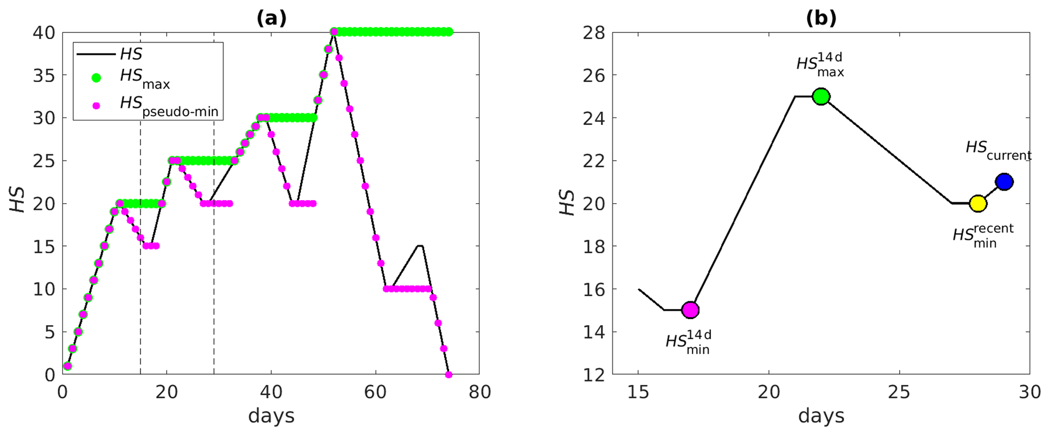
Figure 1 Schematic representation of snow depth HS extreme values used to compute fSCA for a grid cell. (a) To determine fSCA_season, extremes in HS (black line) are tracked over the entire season. When HS decreases, the seasonal maximum snow depth HS_max (green dots) remains constant until a new maximum is reached with subsequent snowfalls. The pseudo-minimum HS_pseudo-min (pink dots) decreases when HS decreases until the next snowfall. It then remains constant until HS either exceeds HS_max or decreases below the previous minimum. (b) To determine fSCA_nsnow, several extremes in HS (black line) are tracked within the last 14 d (dashed black lines in a): the current value HS_current (blue dot), the minimum within the last 14 d HS${}_{\text{min}}^{\text{14\hspace{0.17em}d}}$ (pink dot), the maximum within the last 14 d HS${}_{\text{max}}^{\text{14\hspace{0.17em}d}}$ (green dot) and the minimum prior to the most recent snowfall HS${}_{\text{min}}^{\text{recent}}$ (yellow dot).

For the rare, completely flat grid cells, i.e., a subgrid mean slope angle of zero, Eq. (2) would always result in fSCA =1. In those cases, we therefore use Eq. (4) instead of Eq. (2) to compute fSCA_season.

2.2.2 fSCA_nsnow

To account for possible increases in fSCA after recent snowfalls, we evaluate fSCA (Eq. 1) using ${\mathit{\sigma }}_{\mathrm{HS}}^{\text{Egli}}$ (Eq. 4) computed with differences in snow depth dHS (only positive changes) within the last 14 d (Fig. 1b). We use dHS rather than HS to only account for the contribution of new snow on changes in fSCA, thus as if the new snow fell on bare ground. A time window of 14 d provided reliable fSCA results after intensive testing, but the length of this period may require further investigation once more is known about changes in snow depth distributions in mountainous terrain after snowfall.

Within the 14 d time window, we compute two different fSCA values and then retain the maximum value. First, we evaluate fSCA${}_{\text{nsnow}}^{\text{14\hspace{0.17em}d}}$ using the largest positive change in snow depth within the last 14 d:

$$\begin{array}{}\text{(6)}& {\mathrm{fSCA}}_{\text{nsnow}}^{\text{14\hspace{0.17em}d}}=\tanh \left(\mathrm{1.3}{\displaystyle \frac{\left({\mathrm{HS}}_{\text{current}}-{\mathrm{HS}}_{\text{min}}^{\text{14\hspace{0.17em}d}}\right)}{{\mathit{\sigma }}_{{\mathrm{dHS}}^{\text{14\hspace{0.17em}d}}}^{\text{Egli}}}}\right).\end{array}$$

Here, HS_current is the snow depth at the current time step (blue dot in Figure 1b), HS${}_{\text{min}}^{\text{14\hspace{0.17em}d}}$ is the minimum snow depth in the last 14 d (pink dot in Fig. 1b), and ${\mathit{\sigma }}_{{\mathrm{dHS}}^{\text{14\hspace{0.17em}d}}}^{\text{Egli}}$ is computed using the maximum difference in snow depth dHS${}^{\text{14\hspace{0.17em}d}}={\mathrm{HS}}_{\text{max}}^{\text{14\hspace{0.17em}d}}-{\mathrm{HS}}_{\text{min}}^{\text{14\hspace{0.17em}d}}$ in the last 14 d, with HS${}_{\text{max}}^{\text{14\hspace{0.17em}d}}$ the maximum snow depth in the last 14 d (green dot in Fig. 1b).

Second, we evaluate fSCA${}_{\text{nsnow}}^{\text{recent}}$ using only the most recent change in snow depth within the last 14 d:

$$\begin{array}{}\text{(7)}& {\mathrm{fSCA}}_{\text{nsnow}}^{\text{recent}}=\tanh \left(\mathrm{1.3}{\displaystyle \frac{{\mathrm{dHS}}^{\text{recent}}}{{\mathit{\sigma }}_{{\mathrm{dHS}}^{\text{recent}}}^{\text{Egli}}}}\right).\end{array}$$

Here, dHS${}^{\text{recent}}={\mathrm{HS}}_{\text{current}}-{\mathrm{HS}}_{\text{min}}^{\text{recent}}$ is the change in snow since the most recent snowfall, where HS${}_{\text{min}}^{\text{recent}}$ is the minimum snow depth prior to the snowfall (yellow dot in Fig. 1b). The fSCA${}_{\text{nsnow}}^{\text{recent}}$ avoids spatial discontinuities: without this implementation, grid cells with HS > 0 m prior to a recent snowfall may have a lower fSCA value than grid cells where the same amount of new snow has fallen on the bare ground.

Finally, the maximum of fSCA${}_{\text{nsnow}}^{\text{14\hspace{0.17em}d}}$ and fSCA${}_{\text{nsnow}}^{\text{recent}}$ gives fSCA_nsnow for the current time step and a grid cell.

2.2.3 Seasonal algorithm

Over the course of the snow season, we derive fSCA_nsnow and fSCA_season for each time step and grid cell (Fig. 2). The final fSCA was then obtained by taking the maximum of both values. This full seasonal fSCA algorithm, i.e., including the tracking of HS and SWE, was implemented in a distributed snow cover model. The code is publicly available on the WSL/SLF GitLab repository (see Code availability section). The data sets used to evaluate the performance of this algorithm are described in the next section.

Figure 2 Illustration of modeled fSCA${}_{\text{nsnow}}^{\text{recent}}$, fSCA${}_{\text{nsnow}}^{\text{14\hspace{0.17em}d}}$ and fSCA_season for one grid cell over a season. The fSCA is the maximum for each time step from fSCA${}_{\text{nsnow}}=max$(fSCA${}_{\text{nsnow}}^{\text{recent}}$, fSCA${}_{\text{nsnow}}^{\text{14\hspace{0.17em}d}}$) and fSCA_season. All terms are described in Sect. 2.2.

3 Data

3.1 Modeled fSCA and HS maps

We model the snow cover evolution using the JULES investigation model (JIM). JIM is a multi-model framework of physically based energy-balance models solving the mass and energy balance for a maximum of three snow layers (Essery, 2013). While the multi-model framework JIM offers 1701 combinations of various process parameterizations, Magnusson et al. (2015) selected a specific combination that performed best for snowmelt modeling for Switzerland. The latter model combination is used to predict daily snow mass and snowpack runoff for the operational snow hydrology service (OSHD) at WSL Institute of Snow and Avalanche Research SLF. We ran JIM_OSHD at 1 km resolution with hourly meteorological data from the COSMO-1 model (operated by MeteoSwiss) for Switzerland. We used a reanalysis product of daily observed precipitation (RhiresD) from MeteoSwiss, as well as COSMO-1 data. Daily HS measurements from manual observers, as well as from a dense network of automatic weather stations (AWSs), were used to correct precipitation data via optimal interpolation (OI) (Magnusson et al., 2014), which is a computationally efficient data assimilation approach. Using OI in JIM_OSHD, Griessinger et al. (2019) obtained improved discharge simulations in 25 catchments over 4 hydrological years.

To describe the subgrid snow cover evolution in mountainous terrain, our seasonal fSCA algorithm was implemented in JIM_OSHD. As daily values, we used model output generated at 06:00 (UTC). In the following, modeled fSCA and HS maps refer to daily fSCA and HS from JIM_OSHD model output.

Lawrence et al. (2018)Lawrence et al. (2018)

Table 1 Details of the different fSCA algorithms that are compared to the full fSCA algorithm in JIM_OSHD.

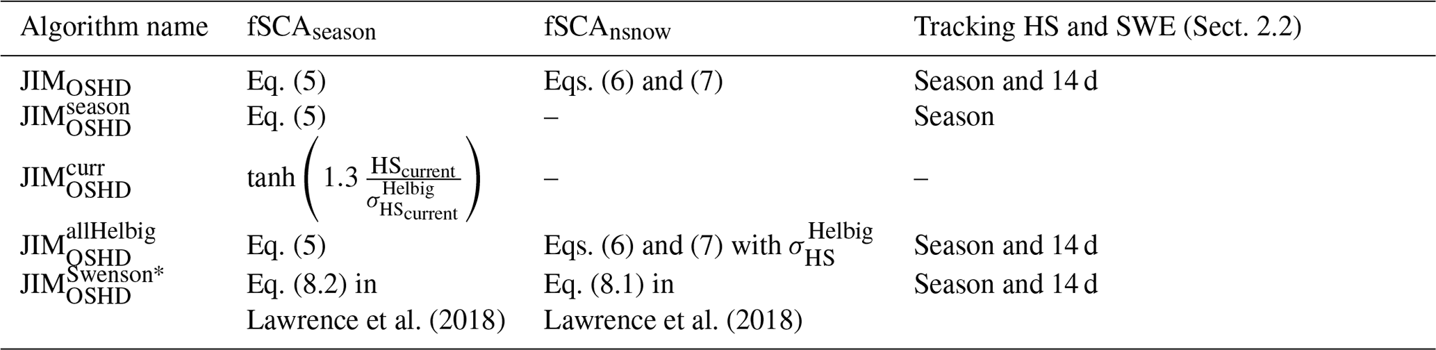
We also computed the snow cover evolution using JIM_OSHD with various simplifications in the seasonal fSCA algorithm, as well as with the fSCA parameterizations implemented in CLM5.0 (Lawrence et al., 2018), which are based on Swenson and Lawrence (2012) (see Table 1 for more details). This latter fSCA algorithm also accounts for hysteresis in accumulation and ablation by using two different fSCA parameterizations and by tracking the seasonal maximum SWE. While subgrid topography is accounted for in the fSCA parameterization during ablation via σ_z, topography is not accounted for during snowfall events. The algorithm of Swenson and Lawrence (2012) was derived by linking daily satellite-retrieved fSCA to snow data. We implemented this algorithm in JIM using our snow tracking algorithm, i.e., the corresponding HS values such as HS_pseudo-min (see Sect. 2.2). This was done to solely evaluate the differences in the fSCA parameterizations. In total, we performed four additional snow cover simulations: JIM${}_{\text{OSHD}}^{\text{season}}$, JIM${}_{\text{OSHD}}^{\text{curr}}$, JIM${}_{\text{OSHD}}^{\text{allHelbig}}$ and JIM${}_{\text{OSHD}}^{\text{Swenson*}}$ (see Table 1).

3.2 Evaluation data

3.2.1 ADS fine-scale HS maps

We used fine-scale spatial HS maps gathered by airborne digital scanning (ADS) with an optoelectronic line scanner on an airplane. Data were acquired over the Wannengrat and Dischma area near Davos in the eastern Swiss Alps during winter and summer (Bühler et al., 2015). We used ADS-derived HS maps at three points in time during one winter season, namely during accumulation on 26 January (acc), at approximate peak of winter on 9 March (PoW) and during ablation season on 20 April 2016 (abl) (Marty et al., 2019). We used a summer DEM from ADS to derive the snow-free terrain parameters.

Each ADS data set covers about 150 km² at 2 m spatial resolution. Compared to TLS-derived (terrestrial laser scan) HS data, the 2 m ADS-derived HS maps had a root mean square error (RMSE) of 33 cm and a normalized median absolute deviation (NMAD) of 24 cm (Bühler et al., 2015).

3.2.2 ALS fine-scale HS maps

We used fine-scale spatial HS maps gathered by airborne laser scanning (ALS). The ALS campaign was a Swiss partner mission of the Airborne Snow Observatory (ASO) (Painter et al., 2016). Lidar setup and processing standards were similar to those in the ASO campaigns in California. Data were acquired over the Dischma area near Davos in the eastern Swiss Alps (see Fig. 3a in Helbig et al., 2021a). We used ALS-derived HS maps at three points in time during one winter season, namely at the approximate peak of winter on 20 March (PoW) and during the early and late ablation season on 31 March and 17 May 2017 (abl), respectively. We used a summer DEM from ALS from 29 August 2017 to derive the snow-free terrain parameters.

Each ALS data set covered about 260 km². The original 3 m resolution was aggregated to 5 m horizontal resolution. Comparing the ALS-derived HS data to manual snow probing within forest but outside canopy (i.e., not below a tree), Mazzotti et al. (2019) reported a RMSE of 13 cm and a bias of −5 cm for 20 March 2017.

3.2.3 Terrestrial camera images

We used camera images from terrestrial time-lapse photography in the visible band. The camera (Nikon Coolpix 5900 from 2016 to 2018, Canon EOS 400D from 2019 to 2020) was installed at the SLF/WSL in Davos Dorf in the eastern Swiss Alps (van Herwijnen and Schweizer, 2011; van Herwijnen et al., 2013). Photographs were taken of the Dorfberg in Davos, which is a large southeast-facing slope with a mean slope angle of about 30^∘ (see Fig. 1 in Helbig et al., 2015a). To obtain fSCA values from the camera images, we followed the workflow described by Portenier et al. (2020). We used the algorithm of Salvatori et al. (2011) to classify pixels in the images as snow or snow-free. Though images are taken at regular intervals (between 2 and 15 min, depending on the year), we used the image at noon to derive fSCA for that day. We evaluated images from five winter seasons (2016, 2017, 2018, 2019 and 2020) every time from 1 November to 30 June.

The resulting snow/no-snow map of the camera images had a horizontal resolution of 2 m. The field of view (FOV) overlaps with four 1×1 km JIM_OSHD grid cells with projected visible fractions between 9 % to 40 % in each grid cell. The camera FOV covers about 0.76 km².

3.2.4 Sentinel-2 snow products

We used fine-scale snow-covered area maps obtained from the Theia snow collection (Gascoin et al., 2019). The satellite snow products were generated from Sentinel-2 L2A and L2B images. We used Sentinel-2 snow-covered area maps over one winter season from 20 December 2017 to 31 August 2018 for Switzerland. We further used Sentinel-2 snow maps over the Dischma area near Davos close to or on the date of the three ALS scans (18 and 28 March and 17 May 2017) and over the Dorfberg area in Davos Dorf from 1 November 2017 to 30 June 2018.

The horizontal resolution of the snow product is 20 m. While the spatial coverage of the Sentinel-2 snow-covered area maps in Switzerland varies every time step, Sentinel-2 may cover several thousand square kilometers. A validation of the Theia snow product with snow depth from AWSs, through a comparison to snow maps with higher spatial resolution, as well as by visual inspection, indicated that snow is well detected, although there is a tendency to underdetect snow (Gascoin et al., 2019). The main difficulty of satellite snow products is to avoid false snow detection within clouds. Furthermore, snow omission errors may occur on steep, shaded slopes when the solar elevation is typically below 20^∘.

Figure 3 Probability density functions after preprocessing for all valid 1 km (a) fSCA, (b) snow depth and (c) elevation per measurement data set. All densities were normalized with the maximum in each data set. Colors represent the different measurement platforms as detailed in Sect. 3.2.

3.3 Derivation of 1 km fSCA evaluation data

For pre-processing, we masked out forest, rivers, glaciers or buildings in all fine-scale measurement data sets. Optical snow products that were obscured by clouds were also omitted. In all fine-scale HS data sets, we neglected HS values that were lower than 0 or above 15 m. We used a HS threshold of 0 m to decide whether or not a 2 or 5 m grid cell was snow-covered. This threshold could not be better adjusted due to a lack of independent observations.

We then aggregated all fine-scale snow data, as well as the snow products from optical imagery, in squared domain sizes L in regular grids of 1 km aligned with the OSHD model domain. For the spatial averages, we required at least 70 % valid data for the fine-scale snow data and at least 50 % valid for the satellite-derived fSCA data in each 1 km grid cell. We excluded 1 km grid cells with spatial mean slope angles larger than 60^∘ and spatial mean measured or modeled HS < 5 cm. We further neglected 1 km grid cells with forest fractions larger than 10 %, derived from 25 m forest cover data. Overall, this led to a variable number of 1 km valid grid cells for the different data sets (Table 2). For the fine-scale snow data sets, this number ranged from 69 to 157 with a total of 668 valid 1 km grid cells. After cloud and forest removal, on average, every second day we had some valid Sentinel-2 data in Switzerland (153 valid days from the 255 calendar days). For the time period from 20 December 2017 to 31 August 2018, this resulted in 216 896 valid 1 km grid cells from a total of 2 274 991 valid OSHD grid cells in Switzerland, i.e., about 9.5 %.

Table 2 Details of the valid 1 km fSCA evaluation data sets after pre-processing as described in Sect. 3.3.

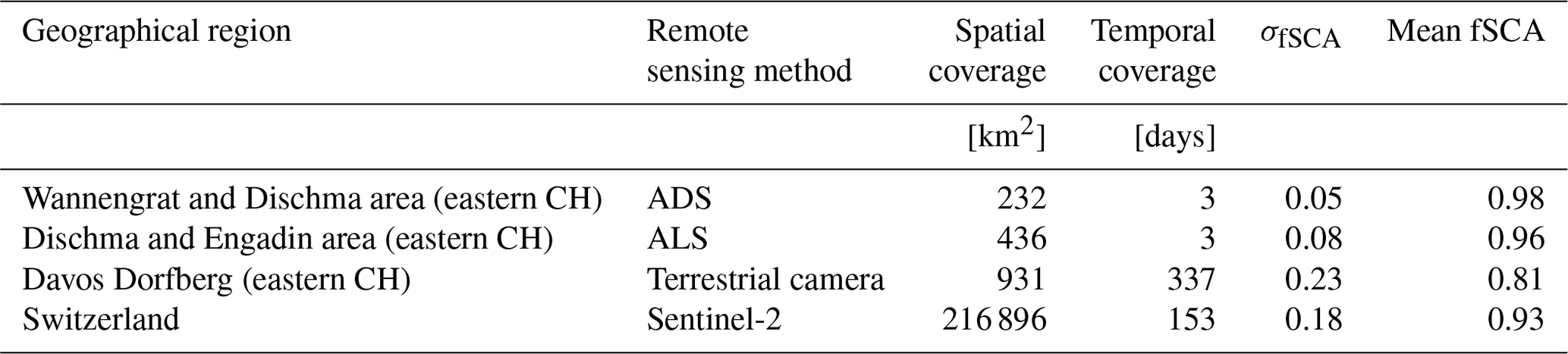
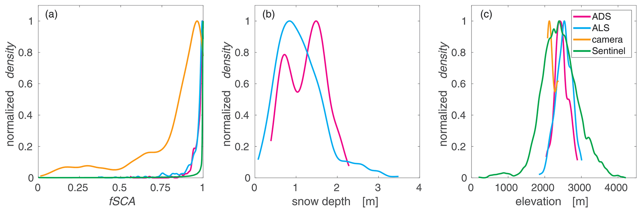
These valid 1 km grid cells covered terrain elevations from 174 to 4278 m, subgrid mean slope angles from 0 to 60^∘ and all terrain aspects. We used three of the four grid cells covered by the FOV of the terrestrial camera since one grid cell had a forest fraction larger than 10 %. On average, every fourth day we had valid camera data (337 valid days from the 1212 calendar days). Valid camera-derived fSCA for five seasons and the three grid cells covered by the FOV resulted in 931 valid 1 km grid cells from a total of 3018 valid OSHD grid cells, i.e., 31 %. The three grid cells have terrain elevations of 2077, 2168 and 2367 m and slope angles of 27, 34 and 39^∘. The diversity in each of the evaluation data sets after pre-processing is indicated in Table 2 and is also shown for valid 1 km domains by means of the probability density function (pdf) for fSCA, HS and terrain elevation z in Fig. 3.

Table 3 Performance measures for modeled fSCA with (I) fSCA derived from all fine-scale HS maps (combined ADS- and ALS-derived fSCA) and (II) Sentinel-derived fSCA (only available for ALS dates). Additionally, performance measures are shown for ALS-derived fSCA with Sentinel-derived fSCA (III) and for modeled fSCA using JIM${}_{\text{OSHD}}^{\text{Swenson*}}$ (IV). Given statistics are NRMSE, RMSE and MPE. For all differences we computed measured minus modeled values respectively Sentinel-derived fSCA minus ALS-derived fSCA for III. The different points in time of the season are specified in Sect. 3.2.

3.4 Performance measures

To evaluate the performance of modeled fSCA compared to the measurements, we used three measures: the root mean square error (RMSE), the normalized root mean square error (NRMSE; normalized by the mean of the measurements) and the mean percentage error (MPE; defined as measured minus modeled, normalized with the mean of the measurements).

4 Results

We present the evaluation of our seasonal fSCA algorithm in three sections: evaluation with fSCA derived from fine-scale HS maps near Davos, evaluation with fSCA from time-lapse photography in Davos Dorf and evaluation with fSCA from Sentinel-2 snow products over Switzerland. We further present some additional comparisons with Sentinel-2 snow products in the first two sections when Sentinel-2 data were available in the Davos area (see Sect. 3.2.4).

4.1 Evaluation with fSCA from fine-scale HS maps

Modeled fSCA compared well with fSCA derived from all six fine-scale HS data sets. Overall, we obtained a NRMSE of 7 %, a RMSE of 0.07 and a MPE of 0.7 % (Table 3). The best performance was for the two dates at the approximate PoW (NRMSE of 2 %, a RMSE of 0.02 and a MPE of 0.3 %), while the performance was somewhat lower during the ablation and accumulation periods.

To investigate the influence of elevation, we binned the data in 200 m elevation bands for the ADS and ALS data sets separately (Figs. 4 and 5). For ADS data, elevation-dependent modeled fSCA values were comparable to the measurements at PoW and early ablation, while the differences during accumulation were more pronounced (compare red and black dots in Fig. 4). There was also no consistent elevation trend, as during accumulation differences between modeled and measured fSCA increased with elevation, while during early ablation the opposite was true. For the ALS data, measurements were only available at PoW and during ablation. Overall, modeled fSCA values were again in line with the measurements (compare red and black dots in Fig. 5). The largest difference was observed for the lowest-elevation bin (0.15 at PoW at 1800 m; Fig. 5a), and for the late ablation data, modeled fSCA was consistently lower than ALS-derived fSCA, in particular for the lower-elevation bins (Fig. 5c).

Valid Sentinel-2 data were only available on dates close to the ALS measurements (green dots in Fig. 5), not to the ADS measurement dates. Overall, modeled and Sentinel-derived fSCA values were in good agreement for the three ALS dates (II in Table 3), there was no clear elevation dependence (compare green and red dots in Fig. 5), and differences were at most 0.05 (for elevations between 2300 and 2500 m in Fig. 5c). The Sentinel-derived fSCA values can also be compared to those from the ALS scans. In this case, the performance measures were somewhat lower (compare II and III in Table 3), and Sentinel-derived fSCA values were especially lower than the ALS data in late ablation (compare green and black dots in Fig. 5c).

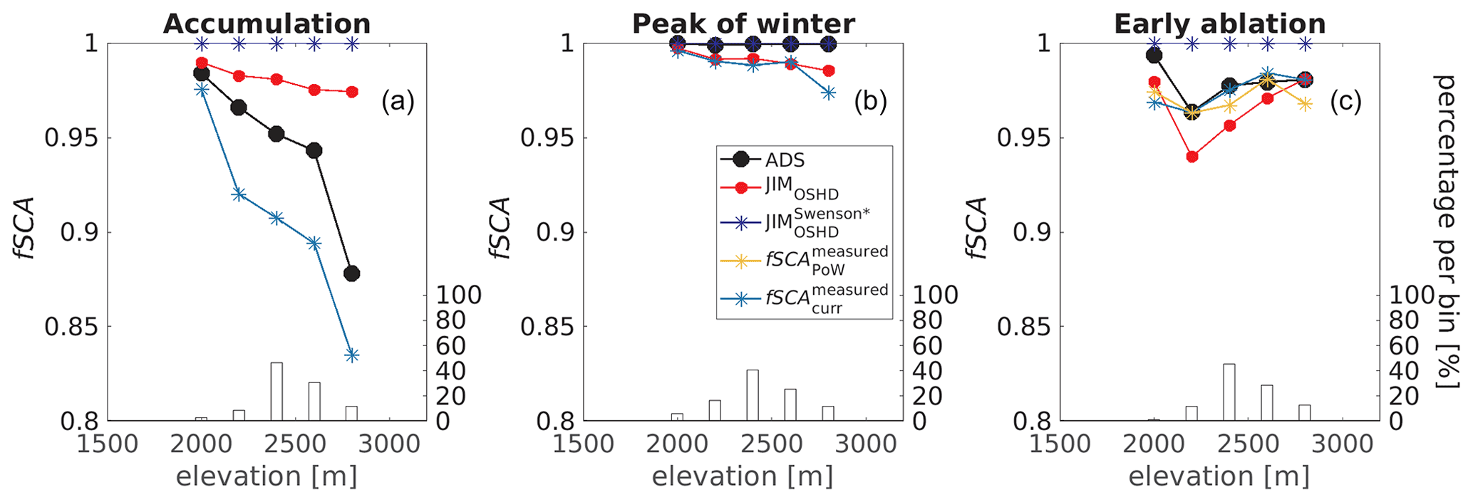
Figure 4 Modeled and ADS-derived fSCA in 200 m elevation bins for three dates: (a) during accumulation, (b) at approximate peak of winter (PoW) and (c) during ablation. Two benchmarks based on Eq. (1) are shown where applicable: fSCA${}_{\text{PoW}}^{\text{measured}}$ (orange stars) uses HS form from the current ADS scan and σ_HS from the ADS scan at PoW, while fSCA${}_{\text{curr}}^{\text{measured}}$ (light blue stars) uses HS and σ_HS from the current ADS scan. The bars show the valid data percentage per bin.

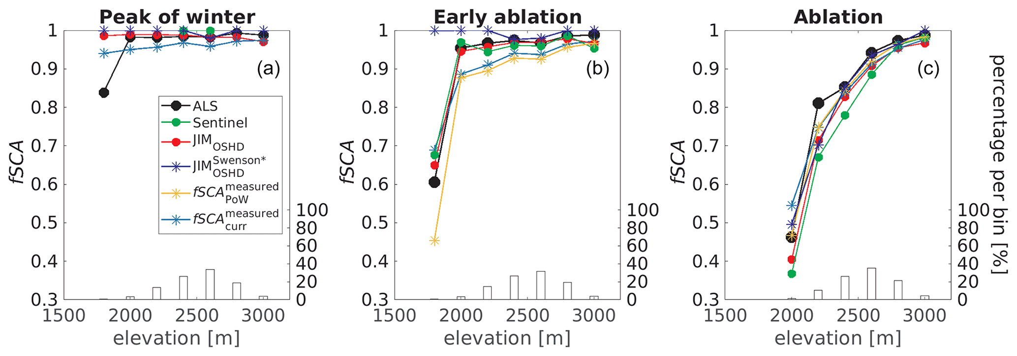
Figure 5 Modeled and ALS-derived, as well as Sentinel-derived, fSCA in 200 m elevation bins for three dates: (a) at approximate PoW, (b) during early ablation and (c) during late ablation. The same two benchmarks based on Eq. (1) as in Fig. 4 are also shown where applicable. Sentinel-derived fSCA (green dots) was available 2 d before the PoW scan, 3 d before the early ablation scan and on the same day as the late ablation scan. The bars show the valid data percentage per bin.

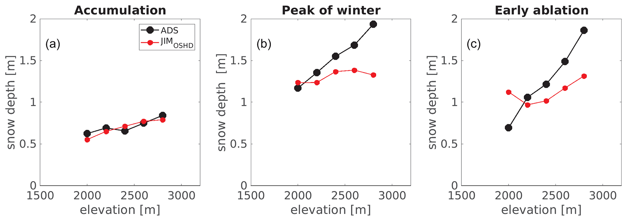
Figure 6 Modeled and ADS-derived HS in 200 m elevation bins for three dates: (a) during accumulation, (b) at approximate PoW and (c) during ablation.

Figure 7 Modeled and ALS-derived HS in 200 m elevation bins for three dates: (a) at approximate PoW, (b) during early ablation and (c) during ablation.

Our seasonal fSCA algorithm is implemented in a complex operational snow cover model framework (Sect. 3.1). Uncertainties related to input or model structure therefore impact modeled HS and fSCA values. To investigate the influence of these uncertainties more closely, we also derived two benchmark fSCA models based on Eq. (1) using measured rather than modeled HS data. The first benchmark fSCA${}_{\text{curr}}^{\text{measured}}$ (light blue stars in Figs. 4 and 5) uses measured HS and σ_HS from the current scan. The second benchmark fSCA${}_{\text{PoW}}^{\text{measured}}$ (orange stars in Figs. 4 and 5) combines current HS measurements with σ_HS values measured at PoW. At PoW, fSCA${}_{\text{PoW}}^{\text{measured}}$ and fSCA${}_{\text{curr}}^{\text{measured}}$ are the same, and fSCA${}_{\text{PoW}}^{\text{measured}}$ can only be derived at or after PoW. Results obtained with both benchmark models were similar except for the lowest-elevation bin in the ALS data set (Fig. 5b and c). Overall, the values of fSCA${}_{\text{curr}}^{\text{measured}}$ were somewhat closer to the measured fSCA values (e.g., Figs. 4c or 5b). Both benchmark models were closest to the measured fSCA values during the ablation season (Figs. 4c and 5c), and overall the agreement was better for higher-elevation bins. Our seasonal fSCA implementation (red dots in Figs. 4 and 5) was also similar to both benchmark models. The largest differences were during the accumulation period (Fig. 4a).

As a final benchmark, we also compared our seasonal fSCA implementation with the parameterizations implemented in CLM5.0 (see Table 1). Modeled fSCA using JIM_OSHD performed better than that modeled with JIM${}_{\text{OSHD}}^{\text{Swenson*}}$ (compare I and IV in Table 3). During most of the season, fSCA values from JIM${}_{\text{OSHD}}^{\text{Swenson*}}$ were close to 1 and showed little elevation dependence (blue stars in Figs. 4 and 5). The only exception was during the late-ablation season, when fSCA values from JIM_OSHD and from JIM${}_{\text{OSHD}}^{\text{Swenson*}}$ were very similar (red dots and dark blue stars in Fig. 5c).

To investigate the origin of the discrepancies between modeled and observed fSCA values more closely, we compared modeled and measured HS in 200 m elevation bins for the ADS and ALS data sets separately (Figs. 6 and 7). For both data sets, modeled HS was substantially lower than measured HS at higher elevations. The only exception was for the accumulation date, when modeled and measured HS values were in good agreement for all elevations (Fig. 6a). For all dates and data sets, the NRMSE between modeled and measured HS was 12 %, and the MPE was 14 %. Note that seasonal variations in ALS HS across all elevations were generally much lower than those in the ADS HS data. This was in part because the time intervals between the three ALS scans (20 March, 31 March and 17 May 2017) were shorter than for the ADS scans (26 January, 9 March and 20 April 2016), and there were also some snowfall events during the ALS ablation period (spring 2017).

4.2 Evaluation with fSCA from camera images

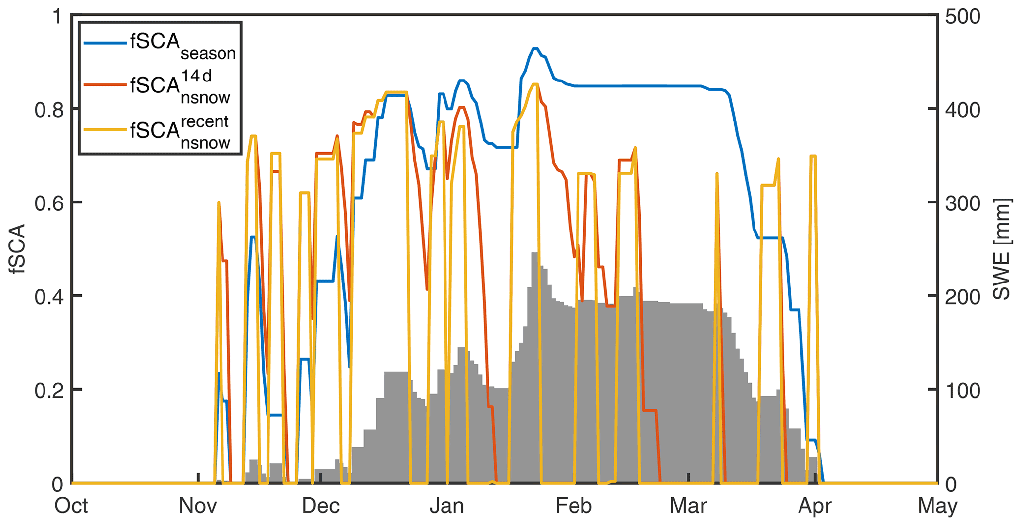
The high temporal resolution of camera-derived fSCA allowed us to evaluate the seasonal model performance. The seasonal trend in modeled fSCA using JIM_OSHD was generally in line with that from camera-derived fSCA (compare red and black dots in Fig. 8). For the grid cell at 2168 m, however, the agreement was somewhat poorer as there was a delay in the modeled start of the ablation season, and modeled fSCA values were too high during accumulation (Fig. 8b, e).

For all winter seasons (2016 to 2020) and for the three grid cells, we obtained a NRMSE of 21 %, a RMSE of 0.17 and a MPE of −7 % (I in Table 4). Note that the inter-annual performance varied substantially, as did the performance among the three grid cells. For instance, for all three grid cells, the overall best performance was for the season 2018 (NRMSE =14 %, RMSE =0.11, MPE $=-\mathrm{4}$ %), while the worst performance was for the season 2019 (NRMSE =25 %, RMSE =0.2, MPE $=-\mathrm{12}$ %).

For winter season 2018, we used Sentinel-derived fSCA to evaluate modeled and camera-derived fSCA values. While overall the agreement between modeled and Sentinel-derived fSCA was good (NRMSE 2 % and MPE of 1 %), the agreement between camera- and Sentinel-derived fSCA was poorer (NRMSE = 12 %, MPE = 5 %). The latter performance values were, however, comparable to the agreement between modeled and camera-derived fSCA for days with valid Sentinel-derived data (NRMSE =12 %, MPE $=-\mathrm{4}$ %).

The camera-derived fSCA was also used to evaluate the relevance of applying our full seasonal fSCA algorithm as opposed to simplifications and JIM${}_{\text{OSHD}}^{\text{Swenson*}}$ (see Table 1 for details). While overall fSCA from JIM${}_{\text{OSHD}}^{\text{season}}$ and JIM_OSHD agreed well, there were substantial differences after snowfall events on partly snow-free ground (compare orange stars and red dots in Fig. 8). Specifically, after such a snowfall event, modeled fSCA using JIM_OSHD generally increased, while JIM${}_{\text{OSHD}}^{\text{season}}$ remained constant. Using JIM${}_{\text{OSHD}}^{\text{curr}}$, modeled fSCA values were less in line with those from JIM_OSHD (compare light blue stars and red dots in Fig. 8). While discrepancies were again large after snowfall events, they were also pronounced during the ablation periods. In general, with JIM${}_{\text{OSHD}}^{\text{curr}}$ the ablation season started later and was followed by a much steeper melt-out period. Using JIM${}_{\text{OSHD}}^{\text{curr}}$ can result in a substantially shorter snow season compared to JIM_OSHD, with a maximum difference of 21 d at 2168 m in the season 2017. Overall, compared to camera-derived fSCA, both simplified models performed less well than JIM_OSHD (Table 4). The performance using JIM${}_{\text{OSHD}}^{\text{allHelbig}}$ was very similar to fSCA from JIM_OSHD; i.e., applying ${\mathit{\sigma }}_{\mathrm{HS}}^{\text{Helbig}}$ instead of ${\mathit{\sigma }}_{\mathrm{HS}}^{\text{Egli}}$ for fSCA_nsnow did not substantially affect model performance. On the contrary, fSCA from JIM${}_{\text{OSHD}}^{\text{Swenson*}}$ had the worst overall performances when compared to camera-derived fSCA (VII in Table 4). Similar to JIM${}_{\text{OSHD}}^{\text{curr}}$, using JIM${}_{\text{OSHD}}^{\text{Swenson*}}$ considerably delayed the ablation season, followed by a much steeper melt out. The snow season was substantially shortened again by at most 32 d in the 2017 season at 2077 m. Modeled fSCA using JIM${}_{\text{OSHD}}^{\text{Swenson*}}$ also largely overestimates fSCA during the accumulation period (blue dots in Fig. 8). Overall, using JIM${}_{\text{OSHD}}^{\text{Swenson*}}$ led to much steeper increases and decreases in fSCA, i.e., an almost binary seasonal fSCA trend that was not in line with camera-derived fSCA.

Table 4 Performance measures for (I) modeled fSCA using JIM_OSHD and camera-retrieved fSCA for the winter seasons 2016 to 2020, (II) modeled fSCA using JIM_OSHD and Sentinel-derived fSCA for the three grid cells for the winter season 2018, (III) camera-derived fSCA with Sentinel-derived fSCA for the three grid cells, and (IV to VII) all JIM-modeled fSCA versions (for details see Table 1), namely for JIM${}_{\text{OSHD}}^{\text{season}}$, JIM${}_{\text{OSHD}}^{\text{curr}}$, JIM${}_{\text{OSHD}}^{\text{allHelbig}}$ and JIM${}_{\text{OSHD}}^{\text{Swenson*}}$, with camera-derived fSCA.

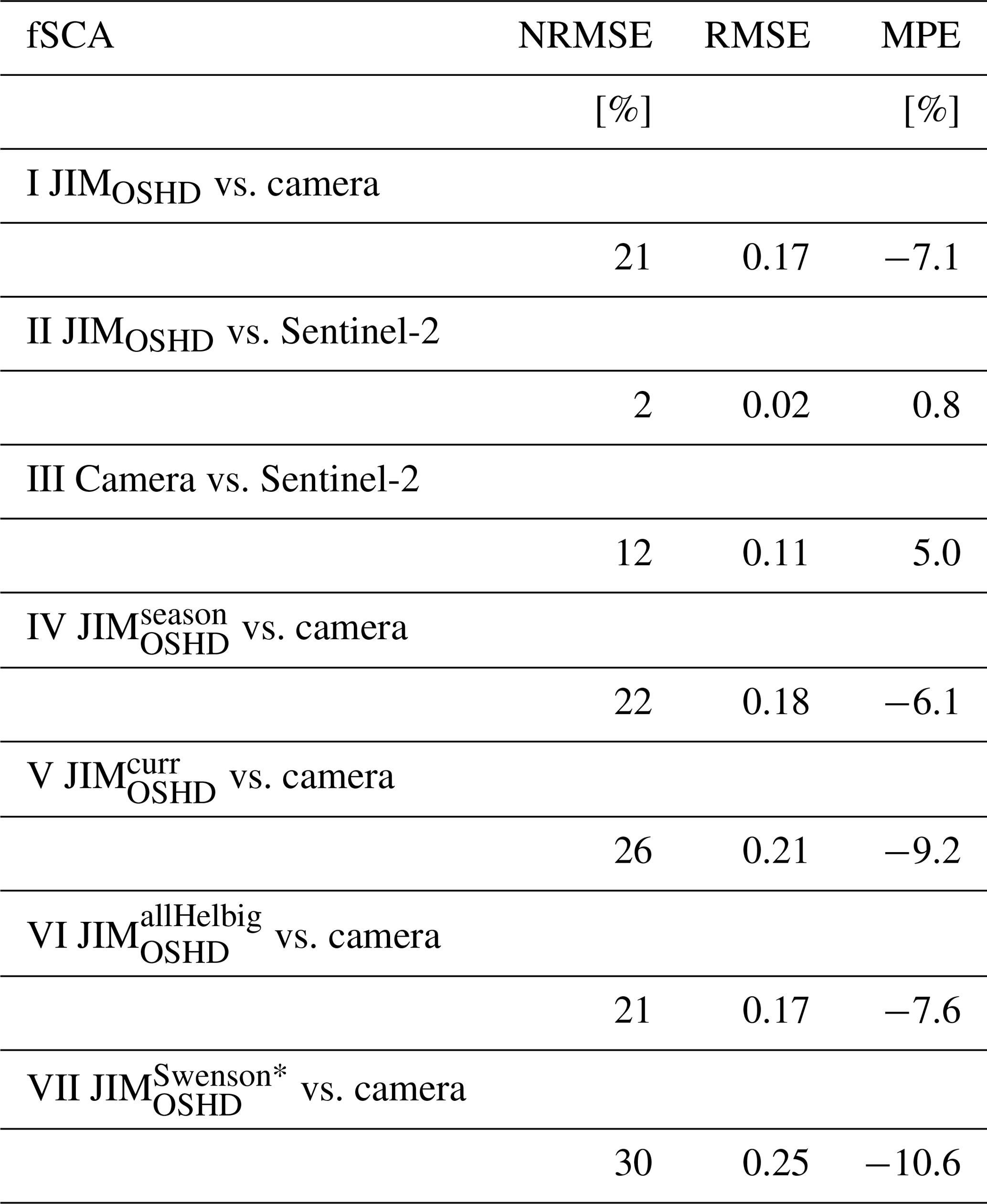
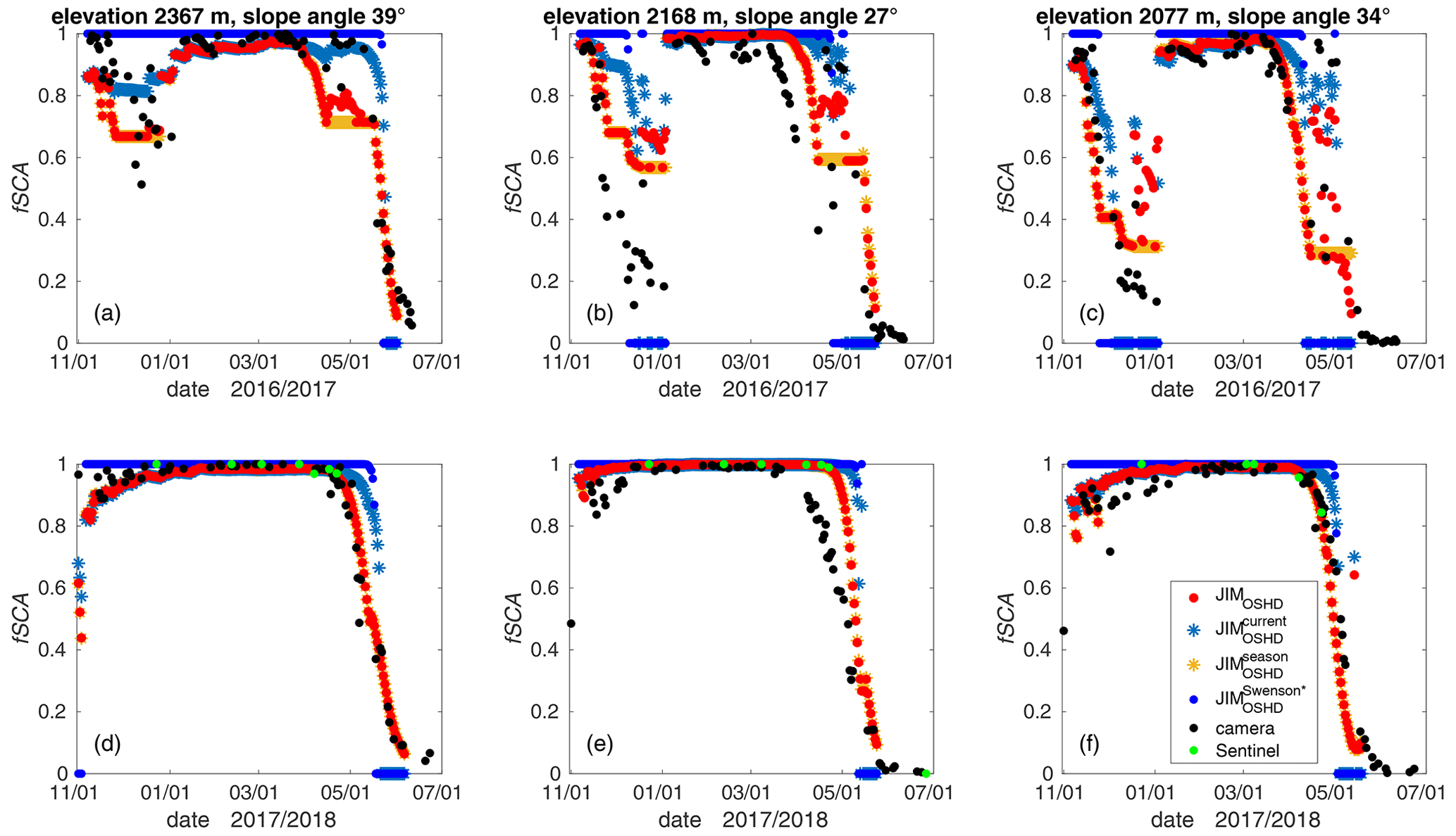
Figure 8 Modeled and camera- and Sentinel-derived fSCA for the three 1 km grid cells within the field of view of the camera for two seasons: (a–c) winter 2017 and (d–f) winter 2018.

4.3 Evaluation with fSCA from Sentinel-2 snow products

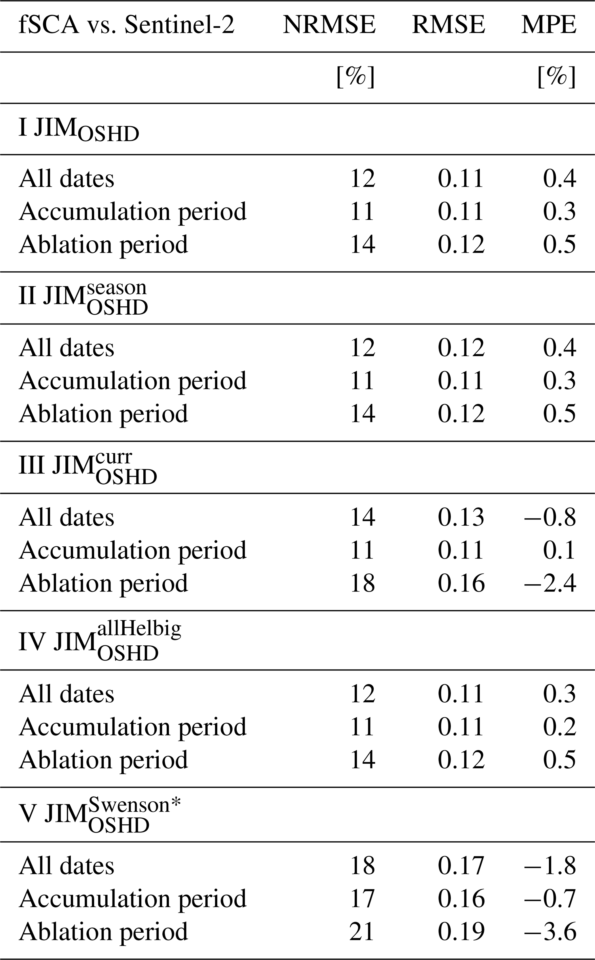
Overall, modeled fSCA using JIM_OSHD compared well with Sentinel-derived fSCA throughout the season (I in Table 5). To investigate the elevation-dependent differences between modeled and Sentinel-derived fSCA in more detail, we binned the data in 250 m elevation bands for each day throughout the entire season (Fig. 9). To estimate the end of the accumulation (1 April 2018) and ablation season (30 June 2018), we used the spatial mean HS (solid black line at bottom of Fig. 9). Overall, differences in performance between the accumulation and the ablation period were small (I in Table 5). However, there were marked differences with elevation throughout the season. Up to the end of the accumulation period, the largest differences between modeled and Sentinel-derived fSCA were at elevations lower than 1500 m, whereas at elevations above around 3000 m, the agreement was good (Fig. 9a). During the ablation period, most of the snow at lower elevations was gone, and modeled fSCA was generally larger than Sentinel-derived fSCA at higher elevations (>2500 m), in particular towards the end of the ablation season. During the summer (30 June to 30 August 2018), i.e., after the end of the ablation season, modeled fSCA was larger than Sentinel-derived fSCA at the highest elevations (>3500 m), whereas between the snow line and these highest elevations, modeled fSCA was generally lower.

Given the high temporal resolution of the Sentinel-derived fSCA data set, we again evaluated the fSCA algorithm simplifications and JIM${}_{\text{OSHD}}^{\text{Swenson*}}$ (see Table 1). Compared to our seasonal implementation, the overall performance values of the fSCA algorithm simplifications were similar except for JIM${}_{\text{OSHD}}^{\text{curr}}$ and JIM${}_{\text{OSHD}}^{\text{Swenson*}}$ (Table 5). Modeled fSCA values with JIM${}_{\text{OSHD}}^{\text{curr}}$ and JIM${}_{\text{OSHD}}^{\text{Swenson*}}$ were generally larger than Sentinel-derived fSCA, resulting in larger MPE values with the largest ones for JIM${}_{\text{OSHD}}^{\text{Swenson*}}$ (compare I, III and V in Table 5). This is also clearly reflected in the elevation-dependent differences between fSCA using JIM${}_{\text{OSHD}}^{\text{Swenson*}}$ and Sentinel-derived fSCA throughout the season (Fig. 9b).

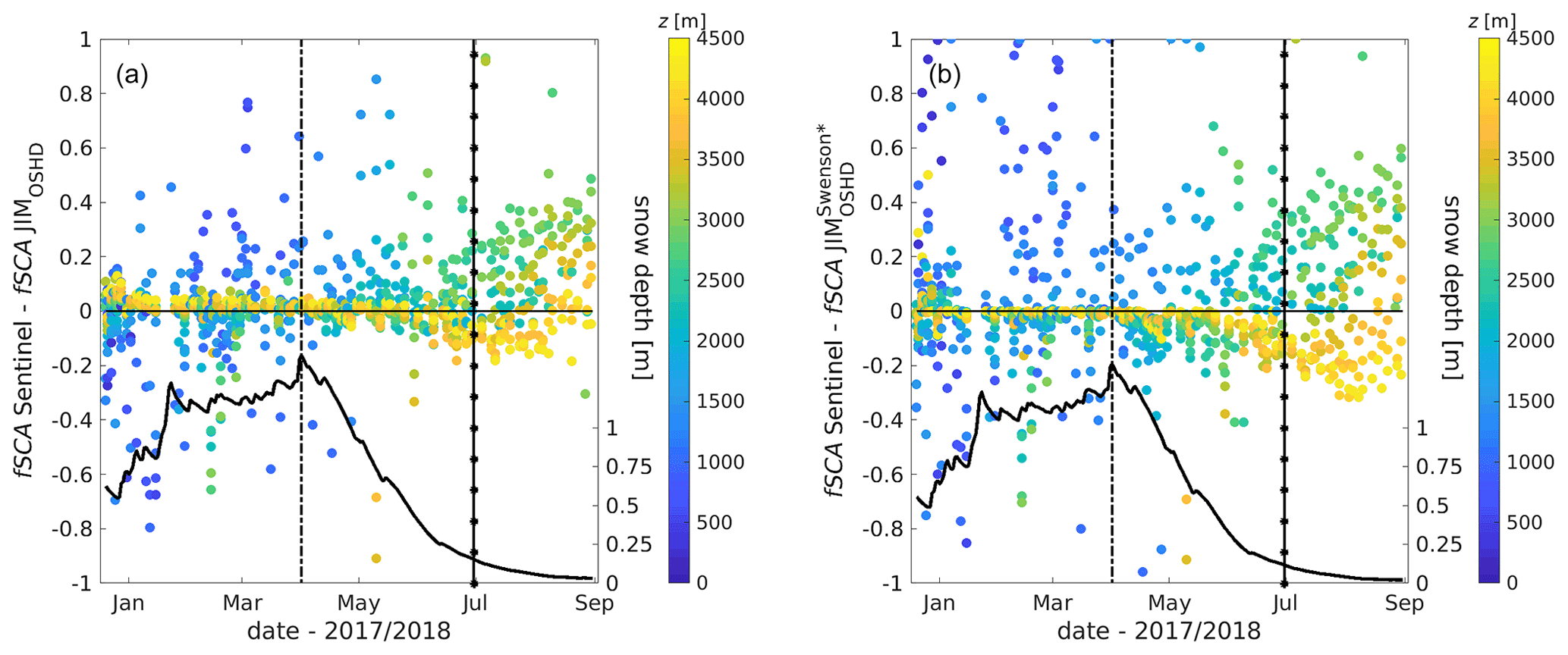
Figure 9 Difference between Sentinel-derived and modeled fSCA for Switzerland as a function of date and elevation z (in 250 m elevation bins) for available satellite dates for (a) JIM_OSHD and (b) JIM${}_{\text{OSHD}}^{\text{Swenson*}}$. Daily spatial mean snow depth HS is also shown (solid black line). The vertical lines indicate the dates for the end of accumulation (dashed) and ablation (line with stars) seasons.

Table 5 Performance measures (I) for modeled fSCA using JIM_OSHD and Sentinel-retrieved fSCA for the winter season 2018 for all valid 1 km grid cells of Switzerland and for all dates (20 December 2017 to 30 June 2018), for the accumulation period (20 December to 1 April), and for the ablation period (1 April to 30 June), as well as (II to V) for all JIM-modeled fSCA versions (for details, see Table 1), namely for JIM_OSHD, JIM${}_{\text{OSHD}}^{\text{season}}$, JIM${}_{\text{OSHD}}^{\text{curr}}$, JIM${}_{\text{OSHD}}^{\text{allHelbig}}$ and JIM${}_{\text{OSHD}}^{\text{Swenson*}}$.

5 Discussion

5.1 Fractional snow-covered area fSCA algorithm

Our seasonal fSCA algorithm is based on the closed-form fSCA parameterization of Helbig et al. (2015a) (Eq. 1) and combines two statistical parameterizations for σ_HS, together with a tracking method, to account for changes in maximum snow depth and precipitation events. The algorithm is modular, meaning that individual parts can easily be complemented or replaced with new parameterizations, e.g., for fSCA_nsnow. Overall, our algorithm only requires subgrid cell summer terrain parameters, which are a slope-related parameter and the terrain correlation length, and tracking snow information.

We evaluated the performance of our seasonal fSCA implementation in Switzerland. We could not explicitly evaluate the performance for completely flat grid cells, i.e., grid cells with a subgrid mean slope angle of zero. After removing rivers/lakes, we only had five 1 km grid cells for Switzerland with a subgrid mean slope angle of zero, i.e., 0.01 % of all grid cells. For these grid cells, using ${\mathit{\sigma }}_{\mathrm{HS}}^{\text{Helbig}}$ (Eq. 2) always results in a fSCA of 1. As a first approach, we therefore proposed to use ${\mathit{\sigma }}_{\mathrm{HS}}^{\text{Egli}}$ (Eq. 4). Although we see no reason why our fSCA algorithm could not be used in other geographic region, it remains unclear at this point if our seasonal fSCA implementation can also be used in flat regions.

We used ${\mathit{\sigma }}_{\mathrm{HS}}^{\text{Egli}}$ (Eq. 4), which does not account for subgrid topography, to derive fSCA_nsnow. We did this to account for uniform blanketing after a snowfall, i.e., to account for possible increases in fSCA after a recent snowfall. When substituting ${\mathit{\sigma }}_{\mathrm{dHS}}^{\text{Egli}}$ with ${\mathit{\sigma }}_{\mathrm{dHS}}^{\text{Helbig}}$ in Eqs. (6) and (7) (JIM${}_{\text{OSHD}}^{\text{allHelbig}}$; see Table 1), the overall performance was very similar (Tables 4 and 5). Thus, while applying ${\mathit{\sigma }}_{\mathrm{dHS}}^{\text{Egli}}$ might not describe the true spatial new snow distribution in mountainous terrain, the formulation is simple and is therefore used here as a first approach. Based on the modular algorithm setup, different closed-form fSCA parameterizations can be applied in our seasonal algorithm, e.g., for a flat grid cell or for fSCA_nsnow (for some empirical examples, see Essery and Pomeroy, 2004).

5.2 Evaluation

5.2.1 Evaluation with fSCA from fine-scale HS maps

The evaluation of the seasonal fSCA algorithm with fSCA from fine-scale HS maps showed that overall the model performed well, especially at PoW (I in Table 3). Modeled fSCA using JIM${}_{\text{OSHD}}^{\text{Swenson*}}$, on the other hand, generally overestimated fSCA (MPE< 0). This algorithm intercomparison shows that the seasonal fSCA evolution is better captured by JIM_OSHD most likely because the JIM${}_{\text{OSHD}}^{\text{Swenson*}}$ model does not sufficiently account for the high spatial variability in snow distribution in complex terrain.

During accumulation at higher elevations, modeled fSCA using JIM_OSHD overestimated ADS-derived fSCA even though modeled HS agreed reasonably well with the measurements (Figs. 4a and 6a). We also used a different model configuration (JIM${}_{\text{OSHD}}^{\text{allHelbig}}$ in Table 1), yet fSCA values did not substantially change for the accumulation date (not shown). Based on this we assume that both σ_HS parameterizations cannot sufficiently describe snow redistribution during accumulation likely due to periods with strong winds following snowfall. The description of σ_HS during the accumulation period thus needs to be improved. This will, however, require more than one spatial HS data set during accumulation.

At PoW and during the ablation season, JIM_OSHD mostly underestimated fSCA compared to fSCA from fine-scale HS maps, without a clear elevation trend (Figs. 4 and 5). Discrepancies between modeled and measured HS, on the other hand, generally increased with elevation (Figs. 6 and 7). Obviously for larger snow depth, correctly modeling HS has little effect on fSCA. The overall underestimated modeled fSCA values were likely a consequence of the HS threshold of 0 m we used to decide whether a 2 or 5 m grid cell was snow-covered or not. In reality, due to measurement uncertainties, both small positive or negative measured HS values can still be associated with snow-free areas. When arbitrarily increasing the HS threshold to ±10 cm for the ALS data, modeled 1 km fSCA values were rather larger than the measurements (not shown). This is not contradictory but emphasizes the need to accurately model HS along snow lines, in which small inaccuracies in HS can have large impacts on fSCA. For instance, during early ablation modeled and measured fSCAs are larger in the lowest-elevation bin than at higher elevations (see Fig. 4c). Unfortunately, we currently do not have detailed snow observations available to define robust HS threshold values which take into account the different points in time of the season, as well as the influence of terrain and ground cover. However, the overall good agreement between Sentinel- and ALS-derived fSCA (Fig. 5 and III in Table 3) provides some confidence in the fine-scale HS data-derived fSCA used here to evaluate modeled fSCA.

The two benchmark fSCA models based on Eq. (1) using measured rather than modeled HS data (fSCA${}_{\text{curr}}^{\text{measured}}$ and fSCA${}_{\text{PoW}}^{\text{measured}}$) generally showed similar trends as HS-derived and modeled fSCA (Figs. 4 and 5). At PoW, fSCA${}_{\text{curr}}^{\text{measured}}$ agreed less well with measured fSCA than our seasonal implementation (see Figs. 4b and 5a). This may indicate uncertainties in the empirical fSCA parameterization (Eq. 1), which requires the further investigation of spatial HS data sets during accumulation. During ablation, we expected that fSCA${}_{\text{PoW}}^{\text{measured}}$ would be closer to measured fSCA than fSCA${}_{\text{curr}}^{\text{measured}}$, which was, however, not the case (see Figs. 4c and 5b). Since the true PoW date is elevation and aspect dependent, we cannot assume that one date for PoW is representative for the entire catchment, covering several hundred square kilometers and large elevation gradients. Thus, measured σ_HS at the date we defined as PoW might not have been representative for the true ${\mathit{\sigma }}_{{\mathrm{HS}}_{\text{max}}}$ in each grid cell as required by Eq. (5). Besides possible uncertainties in the empirical fSCA parameterization (Eq. 1), we assume this is the main reason why these two benchmark models using measured HS data did not outperform our seasonal implementation. Overall, these comparisons emphasize the need for tracking snow information per grid cell, as is done by our seasonal fSCA algorithm.

5.2.2 Evaluation with camera-derived fSCA

The evaluation with fine-scale HS maps revealed overall good model performance at six points in time. It was, however, not possible to comprehensively evaluate the performance over the season. For this, we used daily camera-derived fSCA, showing that the modeled seasonal fSCA trend was mostly in line with observations (Fig. 8).

Model performance compared to the camera-derived fSCA values was overall worse than when comparing to HS-derived fSCA (e.g., NRMSE of 21 % for I in Table 4 compared to NRMSE of 7 % for I in Table 3). Since the higher temporal resolution of the camera data set leads to the largest spread in fSCA values compared to the other two data sets (see Table 2 and Fig. 3), a larger portion of intermediate fSCA values (e.g., close to the snow line) are included which are generally more difficult to model correctly than fSCA values close to 1. The poorer model performance is, however, likely also due to the overall lower accuracy of camera-derived fSCA. For instance, the projection of the 2D camera image to a 3D DEM may introduce errors and distortions. Furthermore, when deriving fSCA from camera images, clouds/fog and uneven illumination, for instance due to shading or partial cloud cover, may deteriorate the accuracy (e.g., Farinotti et al., 2010; Fedorov et al., 2016; Härer et al., 2016; Portenier et al., 2020). Another factor affecting the performance measures was the threshold for the number of valid fine-scale data per 1 km grid cell. When aggregating to 1 km fSCA maps for the Sentinel-derived values, we required at least 50 % valid fine-scale data. This requirement could not be met for camera-derived fSCA as the projected fractions of the camera FOV on the 1 km model grid cells were only 9 %, 13 % and 14 %. This is reflected in the better agreement between modeled and Sentinel-derived fSCA than between camera- and Sentinel-derived fSCA (NRMSE of 2 % vs. 12 % in Table 4). Finally, as the camera was installed at valley bottom, steep slope sections cover larger areas of the FOV, while flatter slope parts remain invisible. This likely led to underestimated fSCA values. On the other hand, valid Sentinel-derived fSCA has a much lower temporal resolution and did not cover the entire ablation period. Instead, Sentinel-derived fSCA was often available throughout the period when fSCA was rather close to 1 (see Fig. 8d, e). Thus, while there is likely more uncertainty in camera-derived fSCA, the high temporal resolution of this product still provides valuable information on model performance throughout the season.

We used the camera-derived fSCA to also evaluate simplifications of our seasonal fSCA algorithm, as well as JIM${}_{\text{OSHD}}^{\text{Swenson*}}$ (Table 1). Compared to our seasonal fSCA implementation, the more simple implementations did not capture the seasonal variation as well (Fig. 8). With JIM${}_{\text{OSHD}}^{\text{curr}}$, the start of the ablation season was delayed, and the ablation season was also considerably shortened by up to 21 d. In this respect, the results for JIM${}_{\text{OSHD}}^{\text{Swenson*}}$ were very similar as overall the increases and decreases in fSCA were very steep, leading to shortened snow seasons and poorer performances (see Table 4). In principle, JIM${}_{\text{OSHD}}^{\text{curr}}$ considers each day as PoW, leading to rapid changes in fSCA, in particular when HS values are low (i.e., early accumulation or ablation season). In JIM${}_{\text{OSHD}}^{\text{season}}$, the seasonal maximum value of HS was additionally tracked, substantially improving the seasonal fSCA trend, in particular during the ablation season. However, changes in fSCA due to snowfall events were still not captured well with this implementation, showing that our new snow tracking algorithm further improves the overall model performance. Since the impact of using JIM${}_{\text{OSHD}}^{\text{allHelbig}}$ on modeled fSCA is mainly restricted to snowfall following melt periods, overall performances were very similar to JIM_OSHD (see Tables 4 and 5). This again indicates that the description of σ_HS following snowfall events requires further investigation.

5.2.3 Evaluation with Sentinel-derived fSCA

By including Sentinel-derived fSCA in our evaluation, we added a data set with both a high temporal resolution and a much larger spatial coverage (see Table 2). The Sentinel-derived fSCA data set comprised about 217 000 1 km grid cells covering a wide range of terrain elevations, slope angles and terrain aspects.

For the investigated winter season, results showed an overall good seasonal agreement across Switzerland, though there was some elevation-dependent scatter (Fig. 9a). Discrepancies during accumulation occurred mostly along the snowline at lower elevations, where lower spatial HS values, as well as more cloudy weather, prevail during accumulation. Both can lead to inaccurate modeled and Sentinel-derived fSCA. Furthermore, we assume that some of the overestimations in modeled fSCA at higher elevations during accumulation could also stem from underestimated σ_HS during periods when strong winds follow snowfall events, as was also observed in the HS data sets (Fig. 4a and Sect. 5.2.1). The scatter at high elevations during ablation and summer likely originates from lower modeled fSCA due to underestimated precipitation as there are fewer AWSs at high elevations for data assimilation in our model.

Performance measures were somewhat poorer than those from fine-scale HS maps (e.g., NRMSE of 12 % for Sentinel vs. 7 % for fSCA for HS data). Uncertainties introduced by reduced visibility in the snow products of Sentinel-2 are the most likely reason for this. Both our camera and the Sentinel-2 data sets cover long time periods at higher temporal resolution; i.e., they include also periods under unfavorable weather conditions. On the contrary, clear sky dates were carefully selected for the on-demand high-quality data acquisitions from the air for our fSCA data sets derived from fine-scale HS maps. Nevertheless, the camera and the Sentinel-2 data sets enabled us to evaluate seasonal fSCA model trends which would not have been possible from only six fSCA data sets derived from HS data.

When evaluating the simplified fSCA algorithms and JIM${}_{\text{OSHD}}^{\text{Swenson*}}$, model performance measures were comparable to our seasonal implementation except for JIM${}_{\text{OSHD}}^{\text{curr}}$ and JIM${}_{\text{OSHD}}^{\text{Swenson*}}$ (Table 5), as was also the case for the comparison with camera-derived fSCA (Table 4). For Sentinel- and camera-derived fSCA, the main reason is likely the limited availability of fSCA data during or shortly after snowfall due to bad visibility and clouds. Additionally, for the Sentinel-derived fSCA, local performance differences across Switzerland are likely averaged out. Nevertheless, fSCA values when using JIM${}_{\text{OSHD}}^{\text{Swenson*}}$ were overestimated compared to Sentinel-derived values (Fig. 9b, and negative MPE for V in Table 5). Similar results were also observed when using JIM${}_{\text{OSHD}}^{\text{curr}}$ (see negative MPE for III in Table 5). These biases are most likely related to the rather steep increases and decreases in modeled fSCA over the season, as we also observed with the camera-derived fSCA (Fig. 8). We further assume that overestimated fSCA using JIM${}_{\text{OSHD}}^{\text{Swenson*}}$ at higher elevations due to underestimating spatial snow depth variability in complex terrain may have compensated for other modeled fSCA error sources (e.g., from underestimated precipitation input at these elevations), leading to an overall lower bias at higher elevations during accumulation compared to our fSCA implementation. Finally, note that the scatter above zero between Sentinel-derived and JIM${}_{\text{OSHD}}^{\text{Swenson*}}$ fSCA (Fig. 9b) almost disappears when we neglect all 1 km domains with modeled HS < 5 cm using JIM${}_{\text{OSHD}}^{\text{Swenson*}}$ (not shown). While the overall NRMSE values for JIM${}_{\text{OSHD}}^{\text{Swenson*}}$ are then comparable to our seasonal implementation (e.g., NRMSE of 12 % for all dates instead of 18 %; see V in Table 5), it reveals the overall overestimation of JIM${}_{\text{OSHD}}^{\text{Swenson*}}$ (e.g., increased negative MPE of −4.1 % for all dates instead of −1.8 %). Clearly, our seasonal fSCA implementation is better suited to more realistically represent seasonal changes in mountainous terrain, in particular following snowfall and during the ablation period.

6 Conclusions

We presented a seasonal fractional snow-covered area (fSCA) algorithm based on the fSCA parameterization of Helbig et al. (2015b, 2021a). The seasonal algorithm is based on tracking HS and SWE values accounting for alternating snow accumulation and melt events. Two empirical parameterizations were used to describe the spatial snow depth distribution: one for mountainous terrain and one not accounting for subgrid topography. An implementation in a multilayer energy balance snow cover model system (JIM_OSHD; JIM, JULES investigation model; Essery et al., 2013) allowed us to evaluate seasonally modeled fSCA for Switzerland.

Compiling independent fSCA data sets with different spatiotemporal characteristics enabled a thorough analysis of the seasonal fSCA algorithm in mountainous terrain of daily 1 km fSCA values. While the evaluation with the three data sets showed overall good seasonal performance, each of the evaluation data sets allowed specific conclusions to be drawn. The evaluation with fine-scale spatial HS-derived fSCA showed that HS uncertainties along the snow line likely contributed most to the underestimation of fSCA during ablation and PoW, emphasizing the need to accurately model HS along snow lines. The camera-derived fSCA data set with the highest temporal resolution confirmed the need for tracking HS over the season, as well as accounting for intermediate snowfalls, to avoid a delayed melt start and a drastic shortening of the ablation season. The Sentinel-derived fSCA data set, with the largest spatial coverage, together with a rather high temporal resolution, demonstrated that the seasonal fSCA algorithm performs well across a range of elevations, slope angles, terrain aspects and snow regimes. This comparison showed that there were some differences at low elevation or along the snowline coinciding with low HS, while discrepancies occurred mostly at high elevations towards the end of the season during summer.

Overall, NRMSEs for seasonally modeled fSCA increased from 7 % for HS data-derived fSCA to 12 % for Sentinel-derived fSCA and to 21 % for camera-derived fSCA. While the large variation in performance measures is likely tied to the various temporal and spatial resolutions of the data sets and measurement uncertainties, it also demonstrates the difficulties in drawing conclusions when evaluating a model algorithm with evaluation data from different acquisition platforms. Nevertheless, this comparison with data covering a wide range of spatiotemporal scales allowed us to obtain a comprehensive overview of the strengths and weaknesses of our seasonal fSCA implementation. We are not aware of any seasonal fSCA implementation that has been evaluated in such detail by exploiting independent HS and snow product data sets at high spatial and temporal resolution.

By implementing the fSCA parameterizations applied in CLM5.0 (Lawrence et al., 2018) in JIM_OSHD, we also evaluated modeled fSCA using JIM${}_{\text{OSHD}}^{\text{Swenson*}}$. This showed that our seasonal fSCA algorithm captures the seasonal variation best and that seasonal variation in JIM${}_{\text{OSHD}}^{\text{Swenson*}}$ was limited. JIM${}_{\text{OSHD}}^{\text{Swenson*}}$ resulted in often overestimated fSCA values likely because the high spatial variability in snow depth distribution in complex terrain is not sufficiently described.

The implementation of the seasonal fSCA algorithm in a model only requires subgrid terrain parameters from a fine-scale summer DEM in combination with tracking HS and SWE for coarse grid cells. The algorithm is set up such that improvements or adaptations of individual algorithm parts can easily be implemented. The PoW fSCA parameterization of Helbig et al. (2015b) forms the centerpiece of the presented seasonal fSCA algorithm. The recent re-evaluation with various spatial PoW snow depth data sets from seven geographic regions showed an overall NRMSE of only 2 % (Helbig et al., 2021a). This detailed evaluation at PoW in different geographic regions, together with the seasonal assessment with the three fSCA data pools presented here, suggests that the seasonal fSCA algorithm may also be used in other geographic regions. However, further investigations, once more spatial HS data sets before and after snowfalls in complex topography become available, would be advantageous for improvements of our seasonal fSCA algorithm, especially during the accumulation period.