Modeling the Greenland englacial stratigraphy

Radar reflections from the interior of the Greenland ice sheet contain a comprehensive archive of past accumulation rates, ice dynamics, and basal melting. Combining these data with dynamic ice sheet models may greatly aid model calibration, improve past and future sea level estimates, and enable insights into past ice sheet dynamics that neither models nor data could achieve alone. Unfortunately, simulating the continental-scale ice sheet stratigraphy represents a major challenge for current ice sheet models. In this study, we present the first three-dimensional ice sheet model that explicitly simulates the Greenland englacial stratigraphy. Individual layers of accumulation are represented on a grid whose vertical axis is time so that they do not exchange mass with each other as the flow of ice deforms them. This isochronal advection scheme does not influence the ice dynamics and only requires modest input data from a host thermomechanical ice sheet model, making it easy to transfer to a range of models. Using an ensemble of simulations, we show that direct comparison with the dated radiostratigraphy data yields notably more accurate results than calibrating simulations based on total ice thickness. We show that the isochronal scheme produces a more reliable simulation of the englacial age profile than traditional age tracers. The interpretation of ice dynamics at different times is possible but limited by uncertainties in the upper and lower boundary conditions, namely temporal variations in surface mass balance and basal friction.

1 Introduction

Summarizing the history of oceanography, Wunsch (2007) describes how the complicated retrieval of observations in the pioneering period caused the field to take on a “geological flavor”. The necessity to combine data from expeditions spanning various decades painted the picture of a largely invariable ocean with constant strata of water mass properties. Later, advances in measurement techniques, most notably the advent of space-borne remote sensing, forced a revision of this view, and it is now widely accepted that the ocean is capable of even abrupt dynamic changes in which the vertical stratification often plays a pivotal role (e.g., Li and Born, 2019). The glacial flow of land ice may be less prone to changing quite as rapidly as the ocean, but the scarcity of data from the ice sheet's interior until recently mirrored that of early oceanography. In this case, air-borne remote sensing provided a first comprehensive dataset using radar soundings (MacGregor et al., 2015b), and it was shown that the structure of this radiostratigraphy also contains information about ice dynamics and how it has changed over time (MacGregor et al., 2016).

Modeling techniques must accompany this progress. The analysis of dynamic signals in the new radiostratigraphy dataset relied on a steady-state model of ice dynamics published 40 years prior (Whillans, 1976), predating the development of all thermomechanical ice sheet models. The spatially comprehensive simulation of englacial layers could help us to select where to drill ice cores in dynamically active regions (EGRIP), to find intact stratigraphy near the glacier bed (Fischer et al., 2013), to reconstruct past accumulation rates by decomposing dynamic thinning from the depositional signal (Waddington et al., 2007), or to determine the origin and age of outcrops near the margins (Higgins et al., 2015). Not least would models greatly benefit from calibration and validation with the new wealth of observational constraints.

Previous efforts to simulate the englacial layering and age profiles in three-dimensional ice sheet models include Eulerian age tracers (Greve, 1997), Lagrangian particle tracking (Rybak and Huybrechts, 2003), and semi-Lagrangian tracer advection schemes (Tarasov and Peltier, 2003). The accuracy of Eulerian tracer advection is severely reduced by spurious diffusion in finite-difference numerical schemes, and fully Lagrangian methods suffer from low particle densities in the most interesting region near the glacier bed. Semi-Lagrangian schemes have seen some success in simulating the three-dimensional stratigraphy of the Greenland ice sheet (GrIS) (Clarke et al., 2005; Lhomme et al., 2005; Goelles et al., 2014). More recent work proposed a fourth approach by simulating layers of equal age, isochrones, explicitly (Born, 2017). Here, the vertical grid is no longer defined in space as, for example, on terrain-following coordinates but in time representing individual periods of accumulation. Over time, isochronal layers will thin as ice flows toward the margins, which allows younger layers to subside, but no flow crosses the vertical boundaries of the grid.

Here we generalize the isochronal modeling approach by addressing its shortcoming and applying it to the entire GrIS. In the formulation by Born (2017), the isochronal model is a stand-alone ice sheet model that calculates all of its properties on the very finely layered isochronal grid. This greatly increases the computational cost with only marginal benefit because most variables such as temperature and velocity do not vary over such small vertical scales. As a consequence, the original isochronal model only covered a two-dimensional section through the GrIS. In this study we will decouple the calculation of the isochrone thickness from the model physics. Information on ice flow is now obtained from the comprehensive thermomechanical model Yelmo (Robinson et al., 2020). This strategy resembles that of Clarke et al. (2005), in which the isochrone model becomes a tracer transport scheme coupled to a conventional model of ice dynamics. One of the major advantages is that the new modularity allows for easy coupling with other ice sheet models.

After a detailed description of the model and experimental setup in Sect. 2, we will show how the simulation of isochrones can be used to constrain an ensemble of transient simulations of the last 160 000 years (160 kyr) in Sect. 3. Individual model parameters, in particular those controlling accumulation at different times during the simulation, create spatially complex patterns of isochrone depth that also differ on the various isochronal surfaces. These additional constraints result in a simulation that is notably different from one that only considers the present-day ice thickness as a tuning target. Comparison of the isochronal tracer scheme with a second-order Eulerian age tracer scheme highlights the shortcomings of the latter. We discuss our results and conclude in Sect. 4, as well as outline future applications.

2 Methods

2.1 The ice sheet model Yelmo

Yelmo is a hybrid ice sheet model which heuristically sums the shallow-ice and shallow-shelf approximations (SIAs and SSAs, respectively) to obtain the ice velocity at a given location (Bueler and Brown, 2009). It is thermomechanically coupled, and it employs Glen's flow law with an exponent of n=3. The model has been run at a horizontal resolution of 32 km with 20 vertical layers. Additional details of the model can be found elsewhere (Robinson et al., 2020); however here we will describe the key model properties that are relevant to this study.

2.1.1 Basal friction

Basal friction at the ice–bed interface is represented with a linear friction law,

$$\begin{array}{}\text{(1)}& {\mathit{\tau }}_{\mathrm{b}}=\mathit{\beta }{u}_{\mathrm{b}},\end{array}$$

with basal velocity u_b and coefficient

$$\begin{array}{}\text{(2)}& \mathit{\beta }={\displaystyle \frac{c_{\mathrm{b}}}{u_{\mathrm{0}}}}N.\end{array}$$

Here, c_b is a unitless two-dimensional field representing the basal properties under the ice, u₀=100 $\mathrm{m}/\mathrm{a}$ is a scaling constant, and N=ρgH is the effective pressure of the ice, disregarding potential contributions from pressurized subglacial drainage systems. N thus evolves with the ice sheet, modifying friction over time, while c_b and u₀ remain fixed. As will be described below c_b is optimized to reduce the mismatch of modeled and observed ice thickness in the present day.

2.1.2 Enhancement factor

Empirical flow laws of ice sheet models are commonly modified with an enhancement factor, E, reflecting changing ice softness depending on flow regime and background climatic conditions (Paterson, 1991; Ma et al., 2010). E evolves in space and time. Slow flow of grounded ice driven by vertical shearing, mainly near the domes, is enhanced due to single-maximum direction fabric growth. In ice streams and ice shelves, preferred directions in the ice fabric are reduced, making the ice stiffer (Ma et al., 2010). Glacial-age ice in vertical-shear regimes has also been observed to be softer than interglacial-age ice due to a higher concentration of impurities that hinder crystal growth, which further enhances flow in these regions (Paterson, 1991). To simulate this in a straightforward way, we consider the enhancement factor as a three-dimensional field defined by two contributions: the reference enhancement factor as defined by the flow regime (E_ref) and additional enhancement resulting from the evolution of the ice sheet in time (E_t):

$$\begin{array}{}\text{(3)}& E=E_{\mathrm{ref}}{E}_{\mathrm{t}}.\end{array}$$

To calculate E_ref, we use three parameters which define the enhancement factor for purely shearing, streaming, and floating regimes (E_shr, E_strm, and E_flt, respectively). In the case of floating ice, it is assumed that no shearing occurs, and so E_ref=E_flt here. For grounded ice, first the fraction of the effective strain rate attributed to vertical shearing is calculated as

$$\begin{array}{}\text{(4)}& f_{\mathrm{z}}={\displaystyle \frac{\left({\dot{\mathit{\epsilon }}}_{\mathrm{xz}}^{\mathrm{2}}+{\dot{\mathit{\epsilon }}}_{\mathrm{yz}}^{\mathrm{2}}\right)}{{\dot{\mathit{\epsilon }}}^{\mathrm{2}}}},\end{array}$$

where ${\dot{\mathit{\epsilon }}}_{\mathrm{xz}}$ and ${\dot{\mathit{\epsilon }}}_{\mathrm{yz}}$ are the shear-strain components of the strain rate tensor, and $\dot{\mathit{\epsilon }}$ is the effective strain rate. Note that f_z is a three-dimensional diagnosed field. The reference enhancement factor for grounded ice is then calculated as the weighted mean between the shear and stream parameter values:

$$\begin{array}{}\text{(5)}& E_{\mathrm{ref}}=f_{\mathrm{z}}{E}_{\mathrm{shr}}+\left(\mathrm{1}-f_{\mathrm{z}}\right)E_{\mathrm{strm}}.\end{array}$$

We set E_strm=1.0 and E_flt=0.7 following Ma et al. (2010), while E_shr is kept as a free parameter for the model evaluation.

Meanwhile, E_t is set to 1 for floating ice and ice streams, representing stiffer ice in these regions as explained above. Ice streams are defined in this context as grounded ice with a velocity magnitude greater than 100 m yr⁻¹. For grounded ice flowing at speeds below this threshold, E_t is treated as a conservative tracer. The surface boundary condition varies in time and is prescribed as

$$\begin{array}{}\text{(6)}& E_{\mathrm{t}}\left(z=z_{\mathrm{s}}\right)={\mathit{\alpha }}_e{E}_{\mathrm{glac}}+\left(\mathrm{1}-{\mathit{\alpha }}_e\right)E_{\mathrm{int}},\end{array}$$

where E_int and E_glac represent the prescribed interglacial and glacial enhancement factors, and α_e is the glacial index shown in Fig. 1. E_t is defined relative to E_ref in that we set E_int=1 and leave E_glac as a free parameter. E_t thus acts as an amplifier to E_ref. The three-dimensional conservative enhancement factor tracer E_t is determined using a second-order, upwind Eulerian tracer scheme.

The resulting enhancement factor field reflects our expectations based on observations. Floating and streaming ice regimes are relatively stiff, while ice in shearing regimes is softer when it is glacial-age ice and undergoing strong shear.

2.1.3 Eulerian age tracer scheme

Yelmo includes an age-tracer advection module that makes use of the three-dimensional Eulerian grid defined by the model. The model actually traces the deposition time at the surface of the ice sheet (upper boundary condition), from which the age can be deduced. At the ice sheet base (lower boundary condition), a flux condition is imposed when basal melting is present, while basal freezing is ignored. The three-dimensional advection equation is solved via an explicit second-order, upwind scheme (Robinson et al., 2020). The scheme has been validated for an analytical one-dimensional vertical column test case with low age errors at the base on the order of 1 %. A more comprehensive comparison with validated results for a three-dimensional test case has not been performed until now. Thus, while the main focus of this paper is based on the use of the independent isochronal layer tracking scheme (see Sect. 2.4 below), the Eulerian ages are also output so that the two approaches can be compared.

2.2 Paleoclimate boundary conditions and surface mass balance

The climate is calculated following a classical snapshot method, in which the present-day climate (PD) and that of the last glacial maximum (LGM) are known (e.g., Greve et al., 1999; Marshall et al., 2000). The climatic forcing for other times is an interpolation of the two snapshots with weighting following a glacial index. The near-surface air temperature field T is thus calculated as

$$\begin{array}{}\text{(7)}& T=T_{\mathrm{pd}}+{\mathit{\alpha }}_{\mathrm{c}}\left(T_{\mathrm{lgm}}-T_{\mathrm{pre}}\right),\end{array}$$

where T_pd is the present-day climatology obtained from a regional climate model simulation, T_lgm and T_pre are results from climate model simulations of the LGM and preindustrial period, respectively, and α_c is the glacial climate index shown in Fig. 1. Precipitation is calculated analogously,

$$\begin{array}{}\text{(8)}& P=P_{\mathrm{pd}}\left({\mathit{\alpha }}_{\mathrm{c}}\left[{\displaystyle \frac{P_{\mathrm{lgm}}}{P_{\mathrm{pre}}}}-\mathrm{1}\right]+\mathrm{1}\right)+{\mathit{\alpha }}_{\mathrm{p}}\mathrm{\Delta }{P}_{\mathrm{hol}},\end{array}$$

although the anomaly scaling is applied as a ratio rather than a sum to avoid negative values. An additional index, α_p (Fig. 1c), is used to impose a spatially constant precipitation anomaly only during the Holocene using the parameter ΔP_hol. This term adds a degree of freedom to the precipitation, which represents atmospheric changes not captured by the available snapshots. The temperature precipitation fields are additionally scaled to be consistent with the dynamic ice sheet topography via a fixed lapse rate of −6.5 K km⁻¹.

The glacial climate index α_c used here is a hybrid of several reconstructions of the Greenland temperature anomaly that span the time period of interest (Vinther et al., 2009; Barker et al., 2011; Dahl-Jensen et al., 2013; Kindler et al., 2014). The individual reconstructions are scaled to match temperature anomalies reconstructed for the NGRIP ice core (Kindler et al., 2014), and then a low-pass filter is applied to remove climate variability at timescales under 10 kyr. Finally, the time series is normalized to give α_c(PD)=0 and α_c(LGM)=1. The glacial index is applied to monthly climate data. Figures 2 and 3 show the mean annual near-surface air temperature and precipitation for PD and LGM. The PD snapshot was obtained as the 1981–2010 climatic average of a simulation of the regional climate model MAR (Fettweis et al., 2008, 2017) forced at the boundaries by the ECMWF ERA-Interim reanalysis (Dee et al., 2011). In the case of temperature, the LGM snapshot is the ensemble mean of simulations contributed to the Paleoclimate Modelling Intercomparison Project Phase III (PMIP3) from several participating models (CCSM4, CNRM-CM5, FGOALS-G2, GISS-E2-R, IPSL-CM5A-LR, MIROC-ESM, MPI-ESM-P, MRI-CGCM3) (Abe-Ouchi et al., 2015). Given the large uncertainty associated with precipitation, we sample the mean ${\overline{P}}_{\mathrm{lgm}}$ and standard deviation σ_P of the PMIP3 simulations to obtain the LGM precipitation snapshot for a given simulation as

$$\begin{array}{}\text{(9)}& P_{\mathrm{lgm}}={\overline{P}}_{\mathrm{lgm}}+f_{\text{LGM}}{\mathit{\sigma }}_P,\end{array}$$

where f_LGM is a free parameter used to scale the uncertainty around the mean. The mean and standard deviation of the LGM precipitation fields are shown in Fig. 3.

Once the monthly temperature and precipitation fields are known for a given time, the surface mass balance is calculated using the positive degree day (PDD) method (Reeh, 1991). Temperatures above the freezing point are converted into melting of snow and ice via the parameters β_s and β_i, respectively. Here β_i=7 $\mathrm{mm}{\mathrm{K}}^{-\mathrm{1}}{\mathrm{d}}^{-\mathrm{1}}$, and β_s is kept as a free parameter. The ice surface temperature is calculated as $T_{\mathrm{s}}=\min \left(T_{\mathrm{ann}}+\mathrm{0.0266}{\dot{m}}_{\mathrm{s}},\mathrm{273.15}\mathrm{K}\right)$, where T_ann is the mean annual near-surface air temperature, and ${\dot{m}}_{\mathrm{s}}$ is the net melt rate at the surface. ${\dot{m}}_{\mathrm{s}}=\mathrm{0}$ m yr⁻¹ when no melting occurs or all melt is refrozen in the snowpack.

Marine-shelf melting is calculated following previous work (Tabone et al., 2018), with the basal mass balance of floating ice calculated as

$$\begin{array}{}\text{(10)}& {\dot{b}}_{\mathrm{shlf}}={\dot{b}}_{\mathrm{ref}}-\mathit{\kappa }\mathrm{\Delta }{T}_{\mathrm{shlf}}.\end{array}$$

Here ${\dot{b}}_{\mathrm{ref}}=-\mathrm{10}$ m yr⁻¹ is a spatially constant shelf basal mass balance representing the PD rate, and κ is a heat-flux coefficient that translates oceanic temperature anomalies into basal melting. Values of κ=10 $\mathrm{m}{\mathrm{yr}}^{-\mathrm{1}}{\mathrm{K}}^{-\mathrm{1}}$ and κ=1 $\mathrm{m}{\mathrm{yr}}^{-\mathrm{1}}{\mathrm{K}}^{-\mathrm{1}}$ are used for shelf ice near the grounding line and the broader shelf, respectively. The oceanic temperature anomaly relative to PD, ΔT_shlf, is calculated as a fraction of the atmospheric temperature anomaly: $\mathrm{\Delta }{T}_{\mathrm{shlf}}=\mathrm{0.25}\left(T-T_{\mathrm{pd}}\right)$ (Golledge et al., 2015); ${\dot{b}}_{\mathrm{shlf}}$ is limited to negative values (i.e., melting) to prevent unrealistic rates of ice accretion during cold climates.

At the lower boundary, the geothermal heat flux Q_geo is imposed with a spatially constant value. It too is a free parameter. Isostatic rebound is calculated dynamically using an elastic lithosphere relaxing asthenosphere (ELRA) isostasy model with a spatially constant time constant set to 3 ka (Ritz et al., 1997). Sea level is spatially constant and varies in time following the global glacial cycle simulation of Ganopolski and Calov (2011) (Fig. 1).

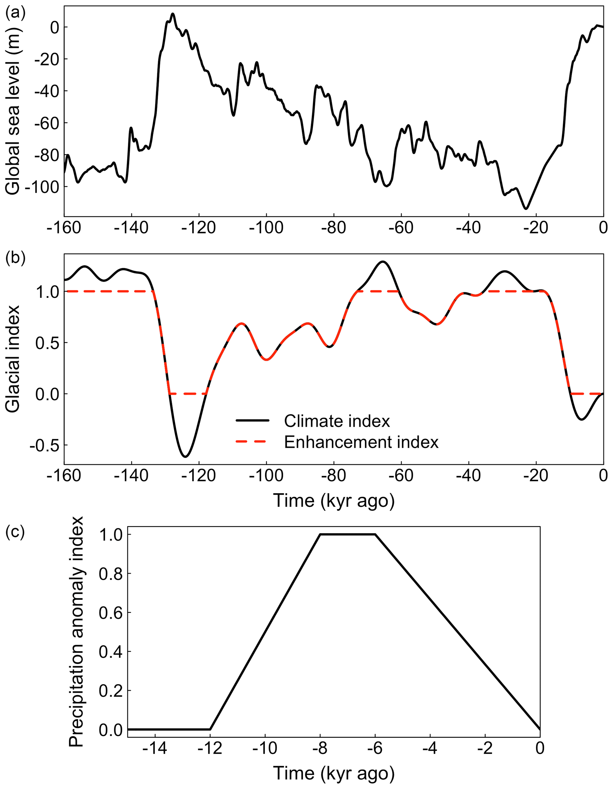
Figure 1 Forcing applied to the simulations. (a) Global sea-level anomaly relative to present day. (b) Glacial indices derived from reconstructed paleo-temperature anomalies over Greenland. The glacial climate index is used to interpolate between the LGM climate snapshot and the present-day climate. The glacial enhancement index is used to interpolate between the imposed enhancement factor for ice during glacial periods and interglacial periods. (c) Holocene precipitation anomaly index scales the imposed ΔP_hol parameter in time to ensure the maximum Holocene precipitation anomaly occurs during the mid-Holocene optimum.

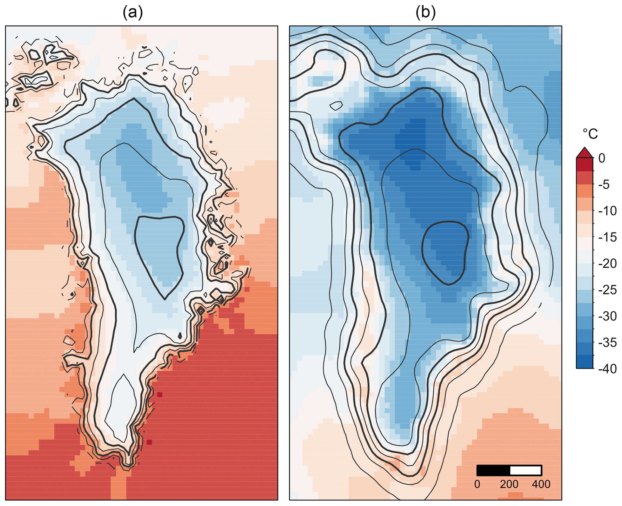
Figure 2 Climate snapshots. Near-surface mean annual air temperature field imposed for present-day (a) and LGM (b) conditions. Present-day data are from a regional climate model simulation (MAR v3.9), averaged over the period 1981–2010. LGM temperatures are the PMIP3 average.

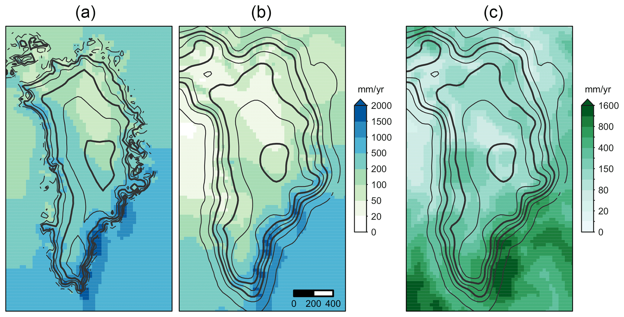
Figure 3 Climate snapshots. Mean annual present-day (a) and LGM (b) precipitation snapshots, along with the uncertainty in the LGM precipitation (c). Present-day climate is the 1981–2010 average from the regional climate model (MARv3.9). LGM precipitation and uncertainty are the mean and standard deviation of model results contributed to the PMIP3 database.

2.3 Spin-up

The spin-up procedure consists of two steps: a temperature spin-up and optimization of the basal friction coefficient field. First, the ice sheet is simulated under constant LGM climatic conditions for 20 kyr using the SIA ice dynamics solver alone, which is mainly intended to spin-up the ice temperature field. Next, the ice sheet is run for another 10 kyr with the full hybrid ice dynamics active. The c_b field used here initially has been tuned to give good results in ice thickness for a steady-state present-day simulation. By the end of this 30 kyr spin-up, the ice sheet extends to near the continental shelf break, in good agreement with the reconstructed LGM ice extent (Lecavalier et al., 2014).

Second, transient simulations from the LGM to PD are performed iteratively, with the basal friction field c_b modified at each iteration to improve the simulated present-day ice thickness following Pollard and DeConto (2012). When the simulation reaches PD, the ice thickness error is calculated ($H_{\mathrm{err}}=H_{\mathrm{sim}}-H_{\mathrm{obs}}$). For each grid point, we then use the upstream H_err to calculate a tuning factor:

$$\begin{array}{}\text{(11)}& \mathit{\epsilon }={\displaystyle \frac{H_{\mathrm{err}}}{H_{\mathrm{0}}}},\end{array}$$

where H₀=1000 m is a scaling parameter controlling the magnitude of changes to c_b for a given iteration. For a given location, H_err is defined as the velocity-weighted average of the upstream values in both lateral dimensions. Also, we limit $\mathit{\epsilon }\in \left(-\mathrm{1.5},\mathrm{1.5}\right)$ in order to avoid scaling c_b too rapidly for large values of H_err. The tuning factor is then used to modify the local basal friction coefficient as

$$\begin{array}{}\text{(12)}& {c_{\mathrm{b}}}^{n+\mathrm{1}}={\mathrm{10}}^{-\mathit{\epsilon }}{c_{\mathrm{b}}}^n,\end{array}$$

where the indices n and n+1 indicate the current and next iteration. Thus, a positive bias in upstream ice thickness H_err results in a reduction of the basal friction coefficient β, which in turn leads to a lower basal velocity for the same basal shear stress (Eq. 2). Once the c_b for the next iteration has been calculated, the model state is reset to the LGM spin-up, and the transient simulation is repeated. We performed 10 iterations, after which the error in simulated PD tends not to reduce further, and the c_b solution is rather stable. The above procedure results in a reasonable internal temperature distribution in the ice sheet that is consistent with the optimized basal friction configuration. This spin-up procedure is applied to each model version in the ensemble method described below.

2.4 The isochronal layer tracing scheme

The tracing of isochronals is based on Born (2017). Key to the successful simulation of the isochronal surfaces is a vertical grid that is defined in time, not space, to avoid vertical advection across grid interfaces and therefore eliminate numerical diffusion. The spacing of this isochronal grid is arbitrary and can in principle be variable, but here we use a constant resolution of 200 years. This means that the domain is virtually empty at the beginning of a simulation, aside from 10 initialization layers. They are inconsequential for the analysis below as they can be regarded as older than 160 kyr and become very thin in the present day. Over the course of the simulation, one additional layer of ice is added every 200 years until the grid is full at the end of the simulation period. Thus, at the end of the simulation, the isochronal grid contains a total of 810 layers. The horizontal grid of the layer tracing scheme is the same as in Yelmo.

A major difference from the original implementation is that the calculation of the ice physics and all boundary conditions are now being handled by Yelmo. The host model provides the two horizontal velocity components, the total ice thickness, and the mass fluxes at the ice surface and the bed to the tracer scheme at every tracer time step, Δt = 5 yr (Fig. 4). These relatively modest requirements make it in principle possible to replace Yelmo with virtually any three-dimensional ice sheet model. The ice velocities are vertically interpolated to the isochronal grid using the vertically integrated layer thicknesses of the latter as reference. This can be done safely with a simple linear interpolation scheme because velocities vary smoothly in the vertical dimension. Inside the isochronal layer scheme, layer thickness is a passive tracer variable that is advected using an implicit upstream scheme and the interpolated velocities. Advection is strictly two-dimensional within each isochrone so that mass is never exchanged along the vertical axis of the isochronal grid. In summary, the isochronal scheme defines depositional age as the grid and layer thickness as an advected property, which is exactly the opposite from Eulerian age tracers that have a grid defined in space and age as a tracer. Our approach therefore eliminates numerical diffusion on the important vertical axis by design.

While interpolation and advection are performed at the Yelmo time step, mass fluxes at the upper and lower boundaries are applied to the tracer scheme at the temporal resolution of the isochronal grid. Between these times, Yelmo mass fluxes are integrated to a temporary buffer. Where the cumulative surface mass balance of the previous 200 years is positive, it defines the thickness of a new layer. Where the mass balance is negative, at the surface and the bed, the appropriate amount is removed from the existing layers. The newly added layer has a thickness of zero in regions of negative mass balance so that older layers naturally outcrop at the surface near the margins. Empty layers below the one that at the current simulation time is the youngest can only be filled by lateral advection within each isochrone even if the local mass balance turns positive.

The less-frequent application of mass fluxes on the isochronal grid causes small discrepancies in the total ice thickness. This effect is very small but with a tendency toward either consistently positive or negative anomalies in certain regions, so it may accumulate over time. To counteract drifting and ensure continuous consistency between Yelmo and the simulated isochrones, we finalize the time step with a normalization to the Yelmo ice thickness.

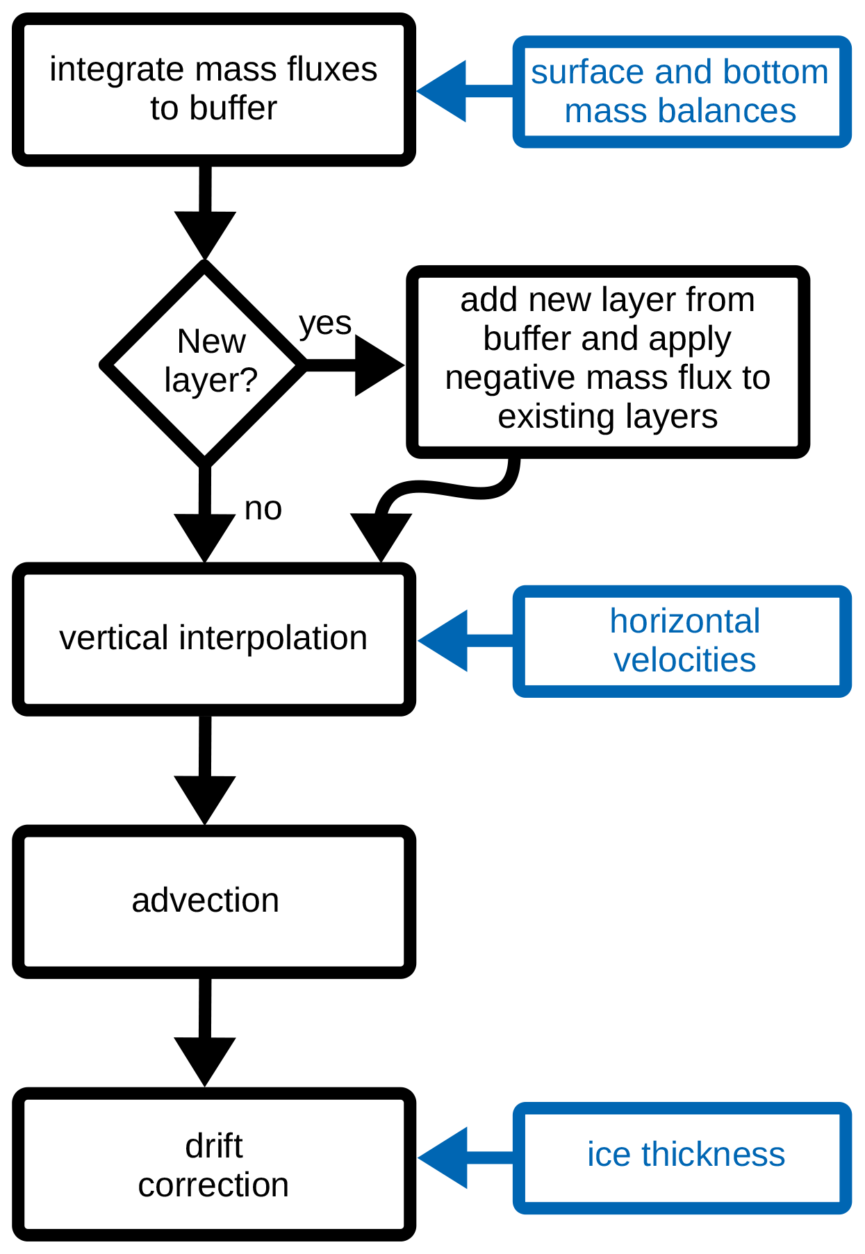
Figure 4 One time step of the layer tracing scheme. Input fields provided by Yelmo are highlighted in blue.

2.5 Ensemble design

An ensemble of 300 simulations were performed to investigate the impact of model and experimental choices on the simulation of isochronal layers. Each simulation consists of the spin-up and c_b optimization procedure described above, followed by simulations of the ice sheet from 160 kyr ago to PD with fully transient boundary conditions. Four model parameters – the PDD factor for snow β_s, the geothermal heat flux Q_geo, and the flow enhancement factors for shearing E_shr and glacial ice E_glac – and two boundary-forcing parameters – the Holocene precipitation anomaly ΔP_hol and the glacial precipitation anomaly f_LGM – were perturbed using a Latin hypercube sampling approach.

3 Results

The skill of the ensemble simulations is quantified by the root mean square error (RMSE) of the ice thickness and the depth of four key isochrones below the surface. The age of these selected isochrones was chosen by the authors of the original dataset (MacGregor et al., 2015a), and their dating is based on a combination of ice core data, in which they intersect radar reflections, as well as the quasi-Nye method. The isochrone data and their uncertainty were then interpolated to the horizontal Yelmo grid. Data uncertainty is not taken into consideration when calculating the RMSE, but this is usually small compared to the data–model mismatch.

In addition to evaluating the ice surface and isochrone depths individually, we also calculate the RMSE across all five evaluation surfaces together as a metric of overall simulation quality. It should be noted that because of the incomplete spatial coverage of the englacial data, ice thickness has a relatively higher weight in the combined RMSE. About 39 % of all points in the combined RMSE are part of the ice thickness field, nearly double of what may be assumed based on it being one of five fields. Only the region with an ice thickness of more than 1000 m is considered to avoid contamination from areas near the ice margin where Yelmo cannot adequately resolve the topography and ice dynamics due its relatively coarse resolution (black contour, Fig. 5).

The presentation of the results is structured to provide a qualitative overview by discussing two examples from the ensemble in Sect. 3.1, followed by a detailed discussion of the full ensemble in Sect. 3.2. The two example simulations are the one with the lowest RMSE for the ice thickness, BEST_ice, and the one with the best skill for the combined RMSE of all five surfaces taken together, BEST_all, to illustrate the benefits of including englacial data.

3.1 Simulation of isochrone depth

The simulated ice thickness and isochrone depths are in qualitatively good agreement with observations in both BEST_ice and BEST_all, but closer inspection reveals important differences. BEST_ice agrees with the observations of ice thickness within a few tens of meters but also shows large disagreements in the depth of the isochronal surfaces (Fig. 5). The contrary is true for BEST_all (Fig.  6). The anomaly pattern of ice thickness of both simulations shows the expected deviations near the ice margin and a mostly homogeneous pattern in the ice sheet interior which do not point to any systematic bias. The anomalies in isochrone depths do show a more detailed pattern of positive and negative anomalies in BEST_all. The positive anomaly in the northwest is visible in all four isochrones and may indicate too much accumulation in the simulation, a too rapid ice flow in this region that includes the ice divide, or both. Similarly, the negative anomaly in the northeast may be interpreted as too little accumulation or a dynamic bias in the model potentially associated with the Northeast Greenland Ice Stream.

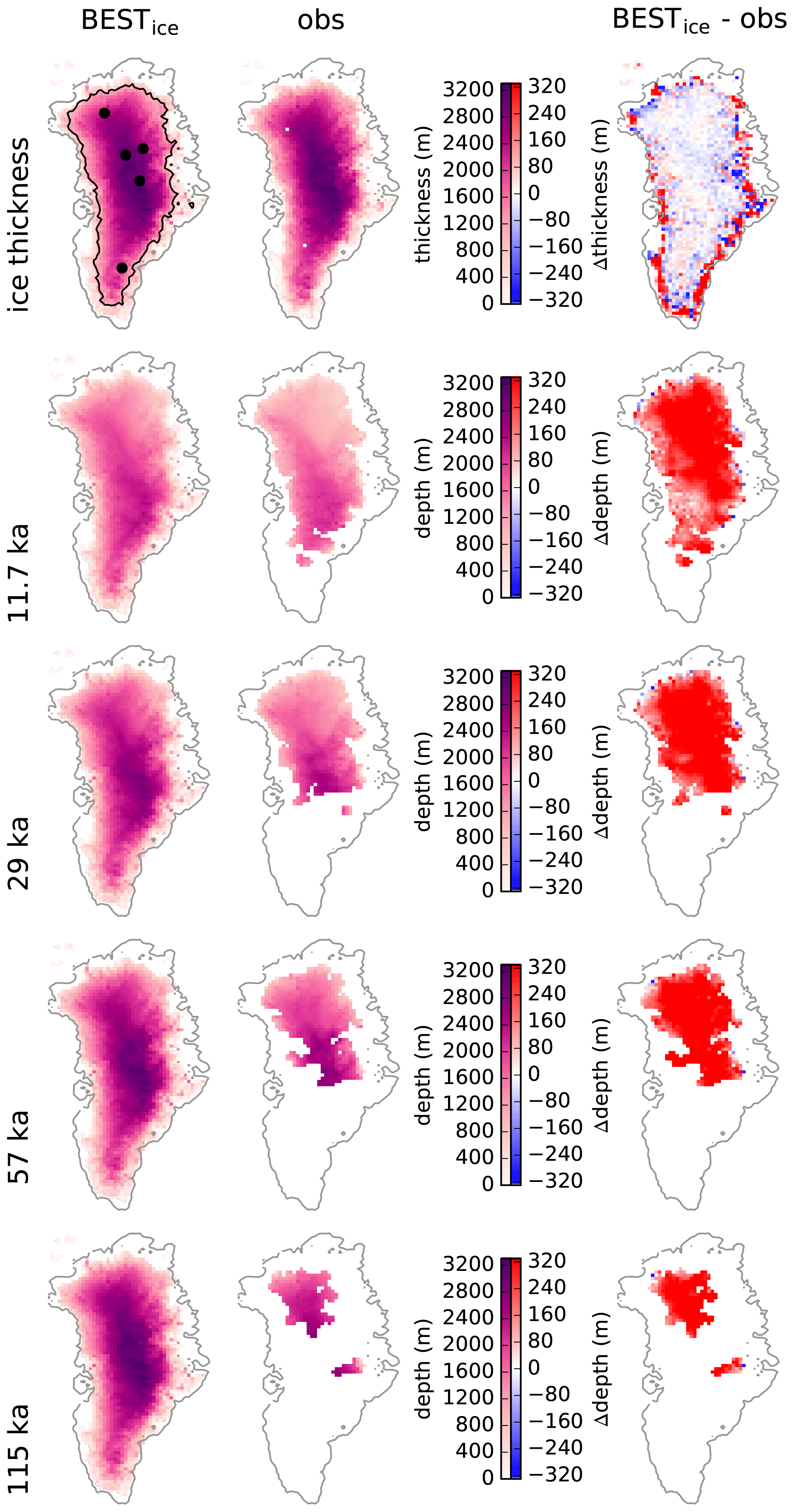
Figure 5 Ice thickness and isochrone depth for the simulation BEST_ice, observations, and the respective differences. Top left panel shows the 1 km ice thickness contour and selected ice core locations from north to south: NEEM, EGRIP, NGRIP, Summit, and Dye-3.

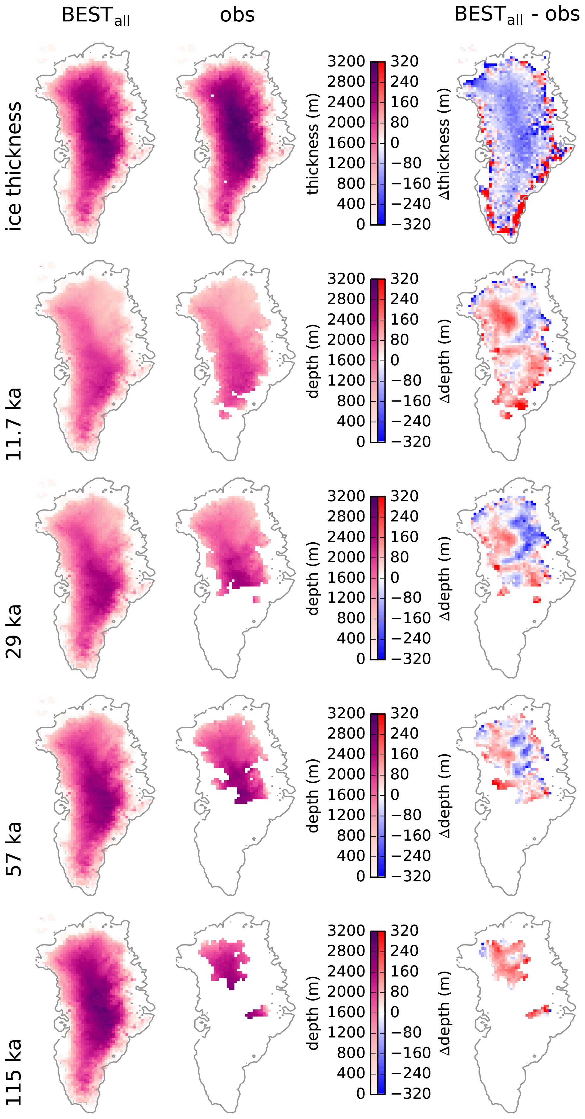
Figure 6 Like Fig. 5, but for simulation BEST_all.

A section through the summit confirms that BEST_ice more closely captures the correct ice thickness but that the englacial stratigraphy is in worse agreement with observations than in BEST_all (Fig. 7). However, looking at the absolute elevation of the isochrones instead of their depth below the surface, it is clear that the relatively good agreement in isochrone depth in BEST_all is largely due to an underestimated ice thickness. This is an interesting result because it suggests that future improvements should focus on the early part of the simulation. We also observe that despite these shortcomings, BEST_all is among the best simulations in simulating the total ice thickness, while BEST_ice shows a low skill in the combined RMSE (Fig. 8). Similarly, the four simulations with the best results for the individual isochrones (indeed four different ones) have reasonably low values for the RMSE of total ice thickness. In contrast to this, the simulation with the best ice thickness performs poorly in all isochrone depths.

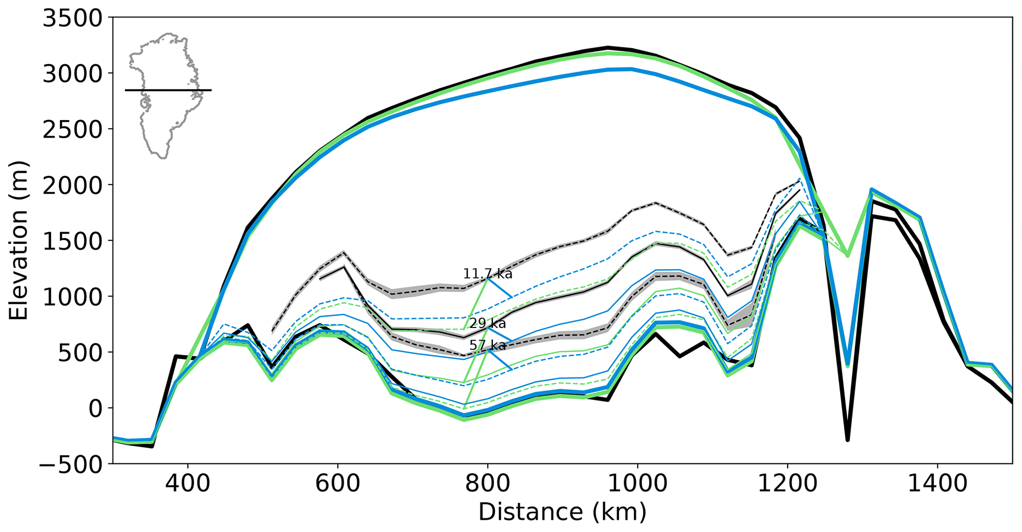
Figure 7 Section through the summit, showing ice surface and bedrock topographies (bold lines), and isochrones (thin lines), each for observations (black), BEST_ice (green), and BEST_all (blue). Isochrones alternate between solid and dashed line styles to improve visibility. Diagonal lines connect corresponding isochrones for the simulations and observations. Reconstruction data for the 115 ka isochrone is not available at this location. Shading is the uncertainty in the observations. Note that distances between isochrones on the elevation scale shown here are not directly comparable to differences in the depth below the surface shown in Figs. 5 and 6.

3.2 Sensitivity to tuning parameters

Not all of the six tuning parameters contribute equally to the ensemble spread (Fig. 8). The Holocene precipitation anomaly ΔP_hol appears to have the largest impact in terms of RMSE for all evaluation surfaces, followed by the scaling factor of the glacial precipitation anomaly f_LGM. The optimal ice thickness is simulated with relatively high values for ΔP_hol, but high Holocene precipitation deteriorates the simulated depth of the isochrones. This appears to be the primary reason behind the large differences between BEST_ice and BEST_all. Lower values of ΔP_hol also worsen the RMSE of isochrone depth, so the optimal value overall is close to 0 m yr⁻¹. All isochrones respond similarly to ΔP_hol because the anomalous precipitation increases their depth similarly. The clear minimum of RMSE in the middle of the parameter range suggests that it was chosen appropriately, although the use of a constant offset for all locations has its shortcomings as will be discussed below.

The scaling of the glacial precipitation uncertainty f_LGM has the strongest impact on the 57 and 115 ka isochrone depths in that both benefit from lower values. The same tendency, albeit weaker, is visible for the 29 ka isochrone depth. The reduced importance is probably due to the relatively short period during which the anomalous precipitation can impact this isochrone. Glacial precipitation has only negligible influence on the 11.7 ka isochrone depth and the total ice thickness. This is to be expected because glacial ice makes up a rather small portion of the total ice thickness.

The influence of the PDD melt factor for snow β_s is mostly limited to the 115 ka isochrone because the preceding period, the last interglacial, is the only time when significant melting occurs in the region above 1000 m. The geothermal heat flux Q_geo and the two enhancement factors E_shr and E_glac have only minor effects. One possible explanation is that these three parameters are most important for ice dynamics that primarily take place near the bed and the ice margins. The deliberate exclusion of the margins but more importantly the very limited coverage of observational data for the deeper isochrones may bias the results to regions where dynamic thinning is least pronounced. In addition, the basal friction optimization may counteract the effects of changing the dynamic parameters because it is carried out for every combination individually. Lastly, the relatively strong impact of the precipitation parameters ΔP_hol and f_LGM can potentially dominate and therefore mask the effects of the other parameters.

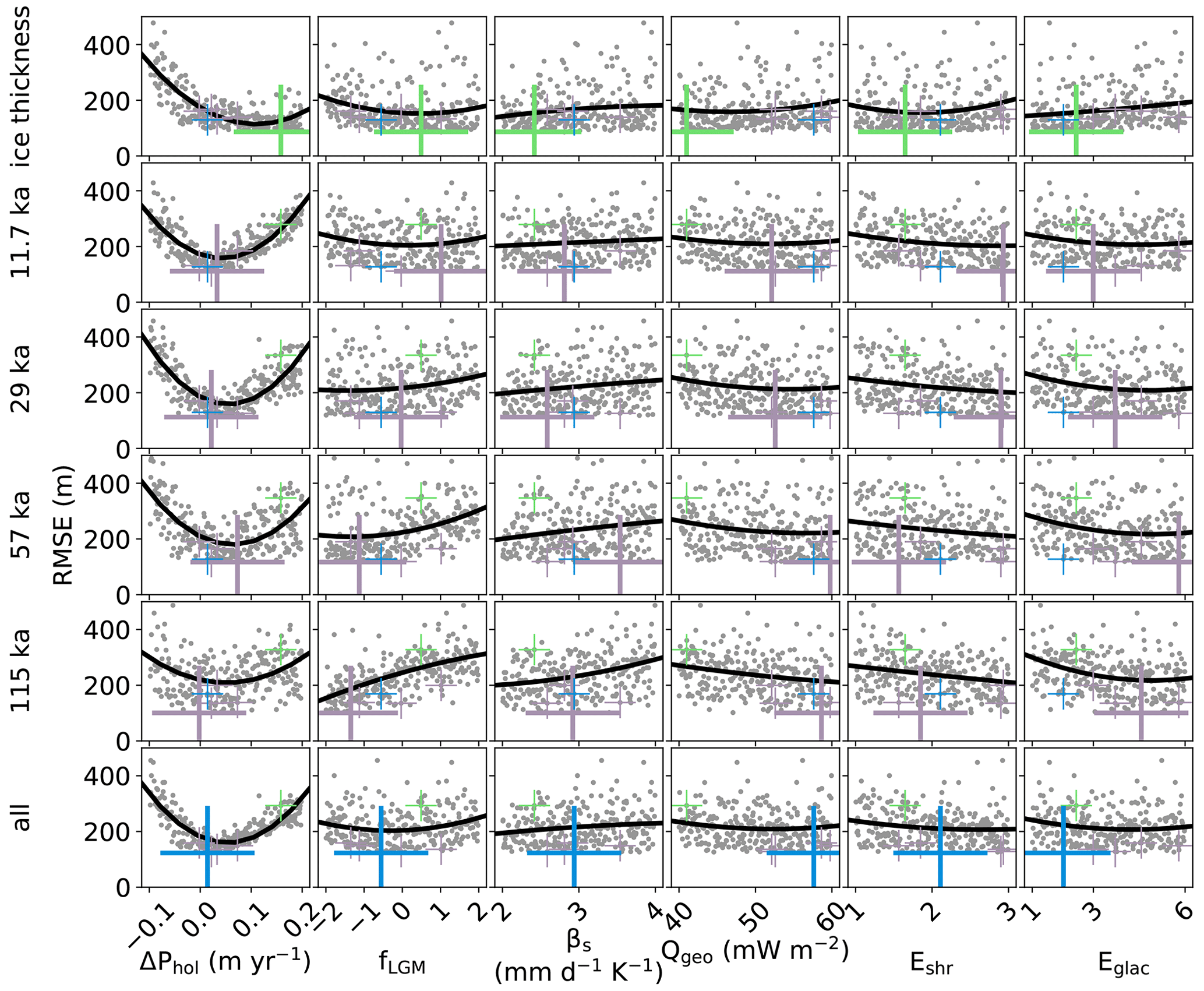
Figure 8 RMSE of ice thickness and isochrone depth for the six tuning parameters. The bottom row shows the RMSE of all isochrones and the total ice thickness together. Individual simulations are marked with gray dots, and large crosses mark the location of the best simulation for each metric as indicated on the left. Smaller crosses of the same color mark the location of the same simulations in the other metrics. A black line illustrates a second order polynomial fit.

The relatively low sensitivity of some of the parameters and the large scatter around the trend lines mean that several simulations across the parameter range produce RMSEs that are comparable to BEST_ice and BEST_all. As a corollary to this finding, although these two sets of parameters produce the optimal results in our ensemble, the parameters themselves are not incontrovertibly optimal (Fig. 9). The best 10 % of simulations agree well on ΔP_hol and f_LGM but otherwise span a large part of the tested parameters range.

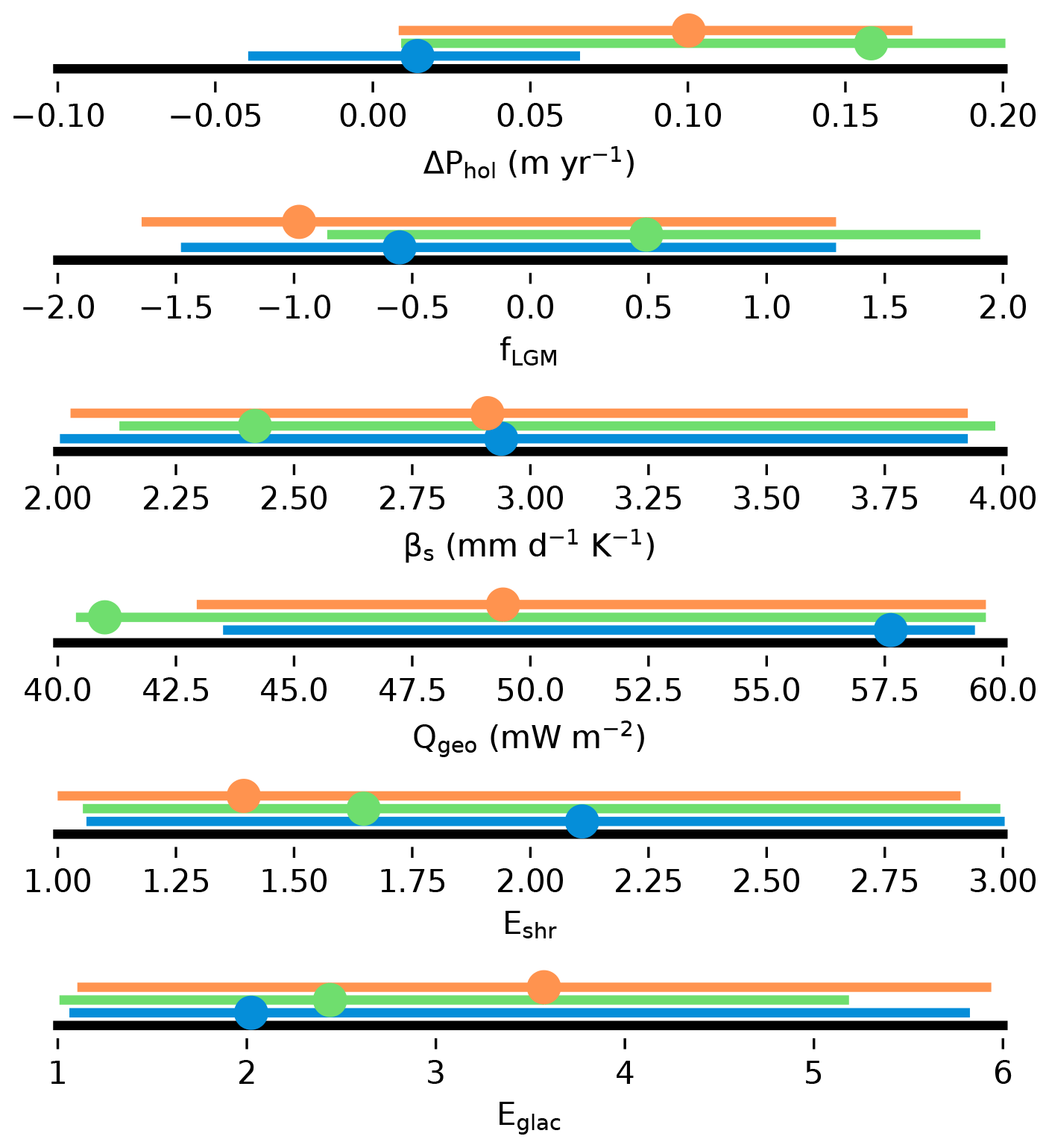
Figure 9 Parameter range for the top 10 % of simulations for the ice thickness metric (green), the combined RMSE (blue), and the combined RMSE based on the Eulerian age tracer (orange). Simulations BEST_ice, BEST_all, and the corresponding optimal simulation for the Eulerian age tracer are highlighted with dots.

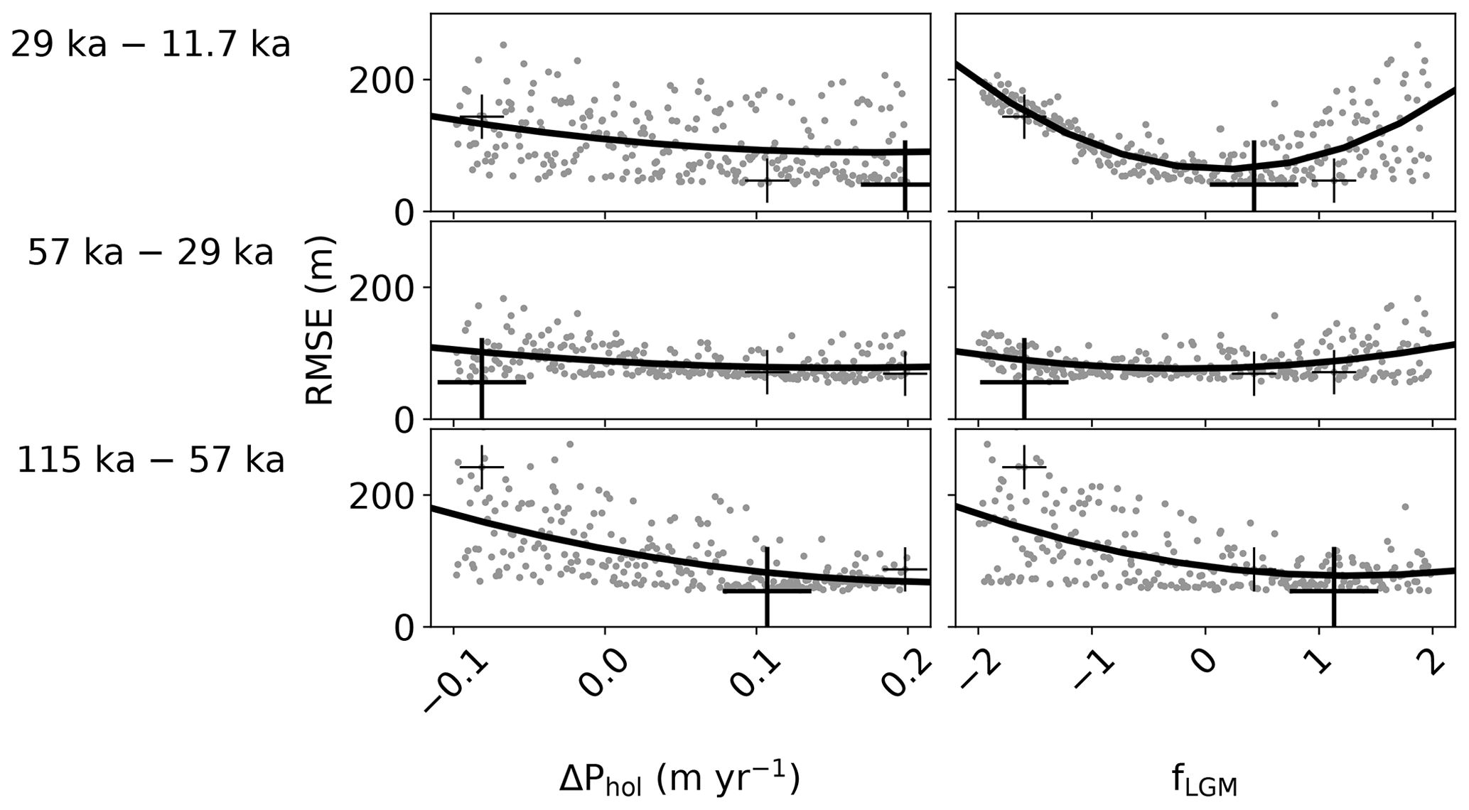
Figure 10 Like Fig. 8, but for differences between isochrones. Note the different scale on the vertical axis.

Additional information can be obtained from the vertical distance between isochrones, not just their depth below the surface (Fig. 10). ΔP_hol does not have a direct effect on these differences, and so they allow inferences on the dynamic response. A higher Holocene precipitation generally has a slight positive effect, in particular on the deepest isochrones, suggesting that they benefit from stronger dynamic thinning. Interestingly, all isochrones agree that a high value for ΔP_hol would be detrimental to their simulated depth below the surface (Fig. 8). We therefore conclude that the imperfect thickness of the layer between the 115 and 57 ka isochrones is due to an unrelated model bias such as an unrealistic surface mass balance (SMB) during that time interval or shortcomings in the simulated dynamics. ΔP_hol may partially counteract these by enhancing dynamic thinning but at the risk of inadvertently combining two errors into one seemingly correct outcome. A similar conclusion can be drawn from the decrease in RMSE of the 115–57 ka difference with higher f_LGM. However, the thickness of the 29–11.7 ka layer, which is directly impacted by the change in glacial precipitation, clearly favors a small value for this parameter.

The RMSE does not provide information on the sign or the spatial pattern of the disagreements. To address this, we also analyze composites for how the evaluation surfaces depend on the high and low values of ΔP_hol and f_LGM. A full discussion is found in Appendix A, but we summarize the main findings here. Even precipitation rates near the upper end of the tested range are barely enough to achieve a sufficiently thick ice sheet. The depth of the internal layers clearly shows the effect of this direct thickening for both ΔP_hol and f_LGM, as well as the dynamic thinning of additional accumulation. The thinning effect is secondary and therefore only visible in layers that do not receive more mass. This also applies to layers that accumulate after the precipitation anomaly, as is clearly seen in the notable shallowing of the 11.7 ka isochrone with high values of f_LGM. The high accumulation before 11.7 ka creates a thicker ice sheet with steeper surface gradients. We find that the precipitation anomalies that result from ΔP_hol and f_LGM are not well suited to improve upon the data–model mismatch found in the ensemble average. However, comparison with reconstructed data may be a way of addressing this issue in future studies.

3.3 Simulated depth profiles, ice volume, and comparison with Eulerian age tracer

While most of the above analysis concerned a spatially comprehensive view of only four isochronal surfaces, the high resolution of our model in the temporal domain allows for a different and complementary analysis using the full age profile at certain locations to constrain model performance (Fig. 11).

All locations show progressive thinning toward the bed, which is more pronounced for regions of high accumulation, as expected. Ice is too young in most of the ensemble simulations probably due to excessive accumulation, in particular at the more southerly locations of Dye-3 and Summit. A less severe mismatch is found for NGRIP, and the simulations agree much better with the reconstructed age profile at NEEM and EGRIP. The most plausible explanation for the difference in simulation quality between north and south is deficiencies in the surface mass balance due to the uncertain climate of the past or the relatively simple parameterization of mass balance used here. However, it is conceivable that the lack of observational isochrone data in the south accentuates these issues or adds to them. For example, the better coverage of radiostratigraphy data in the north biases the PDD melt factor β_s toward this region and its climatic conditions, which likely is a poor choice for the climatically very different south. A similar effect is possible for the parameters that control ice dynamics that may be different for the fast-flowing ice of the south.

BEST_ice has much younger ice everywhere in the ice column due to its unrealistically high accumulation during the Holocene and glacial period. BEST_all achieves a good simulation of the age profiles at NEEM and EGRIP, including periods of rapid age increase around 29 ka and between 60 and 70 ka that agree well with the radiostratigraphy data at the EGRIP site and less so at NEEM.

Comparison of the Eulerian age tracer with the age profile simulated by the isochronal tracing scheme in the same simulation BEST_all (Fig. 11, dashed and solid blue, respectively) shows a clear disagreement, although the two diagnostics should ideally be identical because they simulate the same variable in the same simulation using two different methods. We observe that the Eulerian tracer data generally show a weaker curvature and almost invariably older ages, and they do not capture the variations in accumulation on shorter timescales, all of which indicate that it is subject to numerical diffusion in the vertical dimension. In the Eulerian age tracer old ages diffuse upward. The isochronal layer tracing scheme circumvents this problem by eliminating flow across layer boundaries and by using a numerically much less complex implementation that only requires advection in the two horizontal dimensions.

The spurious bias toward older ice with the Eulerian scheme has a noticeable effect on model behavior when the calibration is based on its results (Fig. 11, orange). Here we show the ages calculated with the isochronal scheme but derived from output of a simulation using parameters chosen to optimize the quality of fit for isochrones generated with the Eulerian age tracer. Note that this is a different simulation from the one shown in blue (BEST_all) which uses parameters that optimize the fit for isochrones generated by the isochronal scheme. To counteract the upward diffusion of older ages, higher values for Holocene precipitation, ΔP_hol, may seem advantageous (Fig. 9, orange). Following the same explanation, less glacial precipitation and so lower values of f_LGM are necessary to obtain a good match with the reconstructed stratigraphy. Consequently, the simulation with the lowest RMSE based on the Eulerian age tracer produces an ice sheet whose true ages, according to the more accurate isochronal scheme, are younger than observations (Fig. 11, orange). The other ensemble parameters are less well constrained both for the isochronal and the Eulerian age schemes, and differences are negligible.

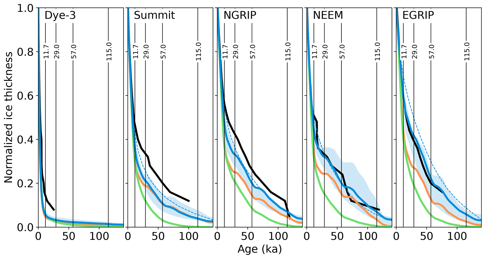
Figure 11 Age profiles of selected ice core locations (see Fig. 5 for map). The curves show radiostratigraphy data (black), BEST_ice (green), BEST_all (blue), and the Eulerian age tracer of BEST_all (dashed blue). The orange curve shows the simulation that produces optimal results for all evaluation surfaces but based on the Eulerian age tracer. The shaded areas are the 10 % best simulations in the combined RMSE, as in Fig. 9.

The tendency toward higher Holocene and lower glacial precipitation in the Eulerian-calibrated simulation is also evident in the total simulated ice volume (Fig. 12). Simulations BEST_ice and BEST_all show a similar ice volume for most of the simulation period, with notable exceptions in the relatively warm Holocene and Eemian. This suggests that the type of calibration has a significant impact on model sensitivity. The simulated ice volume of all simulations is low when compared to earlier reconstructions (e.g., Lecavalier et al., 2014). This is the result of relatively low basal friction in the marine sectors surrounding Greenland and the use of a hybrid ice sheet model, which leads to thinner grounded ice on the continental shelf. Previous ice volume estimates were based on SIA models that generally simulate thicker ice when constrained with the same ice extent. More recent simulations using hybrid models have shown lower volumes on the order of those shown here to be equally possible (Tabone et al., 2018; Buizert et al., 2018). Regardless of this open question, the ice thickness on the continental shelf is of negligible consequence for our comparison with the observed isochrones because they are far inland and not directly influenced by the remote ice margin during the glacial period.

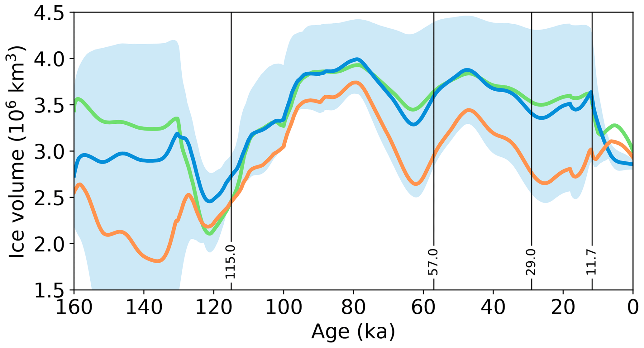
Figure 12 Volume of the Greenland ice sheet as simulated by BEST_ice (green), BEST_all (blue), the 10 % best simulations in the combined RMSE (shading), and the simulation with the lowest combined RMSE based on the Eulerian age tracer (orange). Vertical lines highlight the age of the calibration isochrones.

4 Discussion and conclusions

Our results show that including englacial layers provides useful constraints for the simulation of the GrIS. Simulations that only agree with the modern ice surface topography may produce a very unrealistic ice stratigraphy, suggesting that this calibration objective is too narrow. Given necessary limitations in our model and ensemble design, such as a relatively coarse resolution and a small set of free model parameters, an optimal agreement with both the total ice thickness and isochrone depth appears mutually exclusive. However, simulations that were selected because of their good agreement with the observed isochrone depth show a reasonable simulation of ice thickness, while the opposite is not true. Simulations that are optimized to match the ice thickness require unrealistically high precipitation histories, resulting in erroneous layer ages. These precipitation histories can be ruled out when constraining model parameters with both thickness and layer age.

We find that where ice thickness is above 1000 m uncertainty in surface mass balance has a far greater and more consistent impact on isochrone depth than uncertainty in ice flow parameters. This result may also be influenced by our model's limited ability to simulate the fast ice flow in narrow fjords and near the margins, as well as the poor coverage of isochrone reconstructions in these regions. In addition, the impact of different ice-dynamics parameters is reduced by the optimization procedure for basal friction. However, accumulation directly controls the thickness of isochronal layers, and so it is not surprising that its uncertainty leads to a broad range of simulated isochronal depths.

The simulation of past climates and the calculation of surface mass balance are major sources of uncertainty (van de Berg et al., 2011; Merz et al., 2014a, b, 2016; Plach et al., 2018, 2019) that may be addressed by analyzing the mismatch of simulated and observed isochrone depths. The spatial patterns of these mismatches suggest possible improvements in the distribution of precipitation and melting, in theory at the high temporal resolution of the reconstructed isochrones. Our ensemble of simulations used a spatially uniform Holocene precipitation anomaly and a glacial precipitation anomaly based on differences between global climate model simulations. In addition, we used a simple PDD scheme that calculates SMB from air temperature and total precipitation using empirical proportionality factors. We argue that these choices are justified a priori because their impact could not yet be quantified. The low optimal value for ΔP_hol may be interpreted such that the optimal uniform precipitation anomaly for the Holocene is none at all, but a spatial pattern may nonetheless improve the simulation.

Further work is needed to constrain how parameters impact the flow of ice. In addition to limitations of our specific model, such as its relatively coarse resolution and an assumed significant influence of the basal sliding optimization, we lack a coherent treatment of ambiguous results. As one example, enhanced dynamic thinning appears to improve the simulation of the distance between the 115 and 57 ka isochrones. The results show that this can be achieved with higher values of Q_geo, warming the ice from below and thereby lowering its viscosity, or with higher values of ΔP_hol. Higher accumulation during the last approximately 10 kyr does not directly change the 115–57 ka distance. However, a high ΔP_hol contradicts the findings from the previously discussed analysis of the total isochrone burial depth, and future work should address how to reconcile these results objectively.

Overcoming this current limitation and the possibility to use the explicit forward modeling of isochrones and layer fitting in dynamic regions of the GrIS have the potential to capture spatial and temporal heterogeneity in the basal boundary condition. Possible targets are better constraints on the dynamic impact of basal melting (Fahnestock et al., 2001) and shear margins (Holschuh et al., 2019). Since depositional age has to increase monotonically in the present form of our model, it would be difficult to investigate basal freeze-on and plume formation (Leysinger Vieli et al., 2018), and it is currently impossible to simulate overturning folds (Bons et al., 2019; Wolovick and Creyts, 2016).

Although our isochronal layer tracing scheme adds significant computational cost to the existing thermomechanical ice sheet model, this is mainly due to the much larger number of layers. The flow of mass within isochrones uses an Eulerian scheme that is nearly identical to that of the host model. The higher number of layers and, importantly, preventing flow across vertical grid boundaries result in a notably more reliable simulation of isochrones than using an age tracer on the relatively coarse numerical grid of the host model Yelmo, as shown by our comparison of the two methods within the same simulation. This result is consistent with previous studies (Rybak and Huybrechts, 2003). As a consequence of the dissimilar simulation, the optimal parameters for BEST_all and the simulation that best matches all five evaluation surfaces based on the Eulerian age tracer are very different for the accumulation parameters ΔP_hol and f_LGM. This leads to notable differences in the simulated ice volume and sensitivity to climate change. However, the other four parameters are only weakly constrained in both methods, and so both can be used to exclude the most extreme parameter values. We argue that faced with large uncertainties in boundary conditions, even the less precise Eulerian tracer is sufficiently accurate to provide results better than with no constraint at all, at least for younger isochrones that are less affected by numerical diffusion. Compared to Lagrangian or semi-Lagrangian tracer advection schemes, our method avoids costly interpolation or low particle densities. It is possible to use an uneven spacing of the isochronal grid to concentrate computational cost on key periods of interest.

In summary, the isochronal modeling framework offers a significant step forward in evaluating and calibrating ice sheet models. The method used here is not exclusive to the Yelmo model and can, due to its modest requirements from the host model, readily be adapted to most existing ice sheet models. It is also possible to run the isochronal layer scheme independently from the host model if the necessary fields of ice velocity, mass fluxes, and ice thickness are available at a suitable temporal resolution. We believe that the direct comparison of ice sheet models with one of the best and most comprehensive glaciological archives holds great potential for both future model development and the interpretation of radiostratigraphy data. Large regions of the GrIS, with the important exception of outlet glaciers, will benefit from a better simulation of the SMB because large uncertainties there in accumulation eclipse the impact of dynamics. We plan to use a much more reliable SMB scheme in the future (Born et al., 2019; Fettweis et al., 2020; Zolles and Born, 2021), but these simulations would still depend on uncertain past climates. Here, the isochronal model offers an alternative that is independent from climate simulations. By comparing the simulated isochrones with their observed counterparts, information about past accumulation rates can in principle be derived using inverse modeling (e.g., Waddington et al., 2007; Nielsen et al., 2015). Lastly, future work would greatly benefit from better coverage of the dated radiostratigraphy record in dynamically more active southern Greenland.

Appendix A

Composites of ensemble members with high and low values of the parameter range are shown for the two most sensitive parameters, ΔP_hol and f_LGM, for the five evaluation surfaces and differences between them (Figs. A1 and A2). Both figures are separated into a comparison of the composites with the ensemble average to better understand the sensitivity of the evaluation surfaces to the parameters (left) and with observations (right).

Although high values of ΔP_hol make the GrIS thicker, the simulated ice thickness is always below the observed value. The comparison of the high ΔP_hol composite with the ensemble average shows that the increase in precipitation has its largest impact in the northern part of the ice sheet. Because this region is the driest, the constant offset of ΔP_hol makes the largest relative difference here. As a consequence, isochrone depths show the largest anomalies in the northern and northeastern part like well when compared with the ensemble average.

Comparison of the isochrone depth with observations shows that all isochrones are too deep for the high ΔP_hol composite and too shallow for the low ΔP_hol composite, indicating that the parameter range was chosen adequately. The anomalies of the low ΔP_hol composite with respect to observations have a distinct shape over the north and along the northeastern half of the GrIS. This was also seen in the comparison of the low composite with the ensemble average, but no equivalent is found when comparing the high composite with the observations. This result indicates a nonlinear response to anomalous Holocene precipitation probably due to the flow of ice. Unfortunately, isochrone data from the south are sparse and do not contribute to constraining ΔP_hol. The difference of the ensemble average and observations shows a pattern of both positive and negative anomalies. This may be interpreted as shortcomings in the precipitation data that were used to force the simulations. The comparison with isochrone data could provide a way of addressing this issue in the future.

Regarding the vertical distance between isochrones, a higher Holocene accumulation minimally increases the thickness of the 29–11.7 ka layer (Fig. A1) because ΔP_hol sets in before 11.7 ka (Fig. 1). The older isochrones are all pushed closer together by enhanced dynamic thinning. This effect is especially obvious with anomalously low ΔP_hol, in which the increased isochrone differences in the center are contrasted by a closer vertical distance at the margins because less ice is advected there. In general, the response of the isochrone differences is much less linear than that of their depth below the surface, as seen in the distinct differences between the high-average and low-average differences. The reason for this is that the distance between isochrones that are not directly affected by changes in Holocene accumulation are wholly due to changes in ice dynamics that are known to be highly nonlinear. In contrast, the depth below the surface is a direct and linear consequence of higher precipitation. The comparison of the vertical isochrone distance with observations reveals a heterogenic pattern that does not allow for a robust interpretation at this point.

The composite fields for f_LGM show that the ice sheet becomes thicker with increasing precipitation during the glacial period, but as for ΔP_hol the increase is not enough to achieve a realistic ice thickness (Fig. A2). The thickening is also limited to the center of the GrIS, while the thickness decreases around the margins. This is because the higher accumulation also increases ice flow and therefore the removal of mass. This is especially evident from the depth of the 11.7 ka isochrone that becomes noticeably shallower with high f_LGM. Holocene ice that accumulates on an ice sheet that experienced higher glacial accumulation will experience a thicker ice sheet with steeper slopes which more efficiently remove new ice. The older isochrones all experience the direct effect of higher glacial precipitation, and their depth below the surface therefore is invariably higher for larger values of f_LGM. The pattern of the precipitation anomaly field can be recognized in the isochrone depths (Fig. 3).

The difference in the low f_LGM composite for 29 and 57 ka isochrone depths and the corresponding observations show the fingerprint of the precipitation anomaly pattern (Fig. 3). There is a negative anomaly in the northeast, while the reduction in glacial precipitation is not enough to eliminate the positive isochrone depth anomaly in northwestern Greenland. The pre-Holocene isochrones of the high f_LGM composite are generally too deep (avg–obs), suggesting a negative f_LGM as an improvement, but the imposed glacial precipitation anomaly pattern is not optimal to address spatial heterogeneities. This suggests that this precipitation anomaly pattern is a poor match for the unperturbed model's shortcomings, which is not wholly unexpected because it only represents climate model disagreement.

The vertical distance between isochrones increases with f_LGM for glacial periods, while the oldest layer, 115–57 ka, records the dynamic thinning of the additional load overhead. The positive and negative composites are mostly symmetric when compared with the ensemble average. As for the comparison with observations, clear positive and negative anomalies are found for the high and low composites, so the parameter range has likely been adequately chosen for this particular metric.

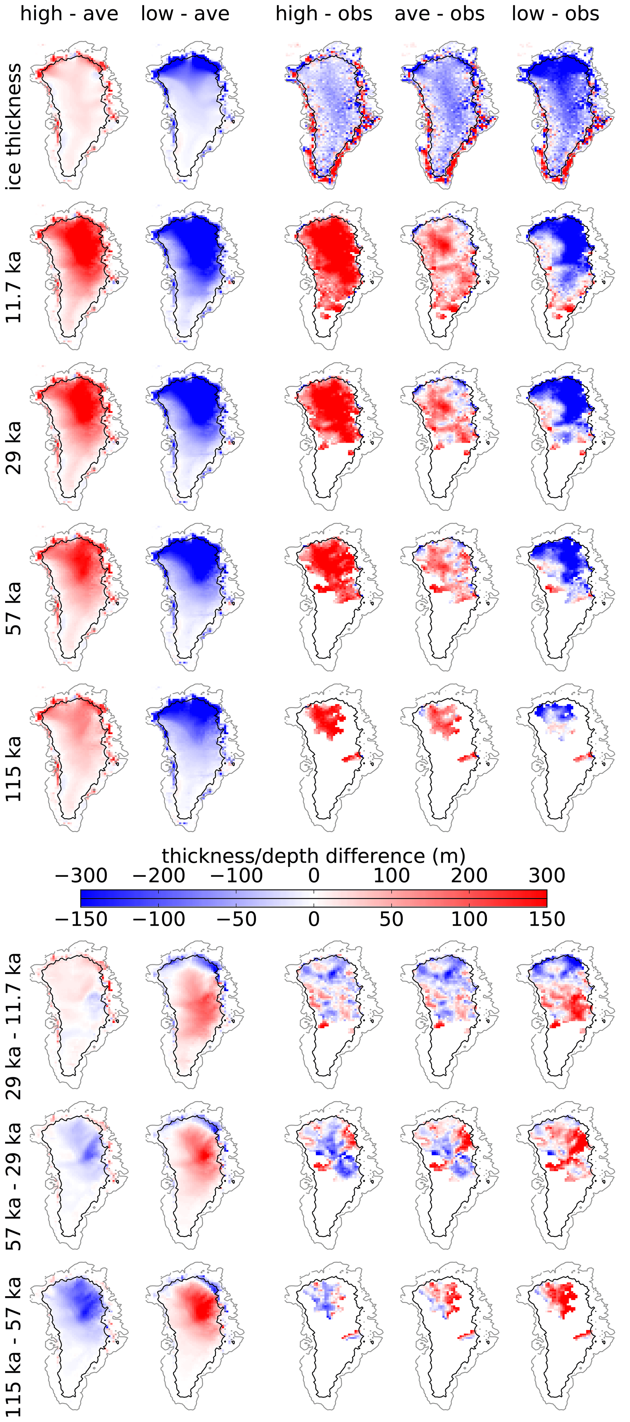
Figure A1 Composite ice thickness and isochrone depth for simulations with high (−0.1 to −0.05 m yr⁻¹) and low (0.15 to 0.2 m yr⁻¹) values of ΔP_hol compared to the ensemble average and observations. A thin black line marks the 1000 m surface elevation.

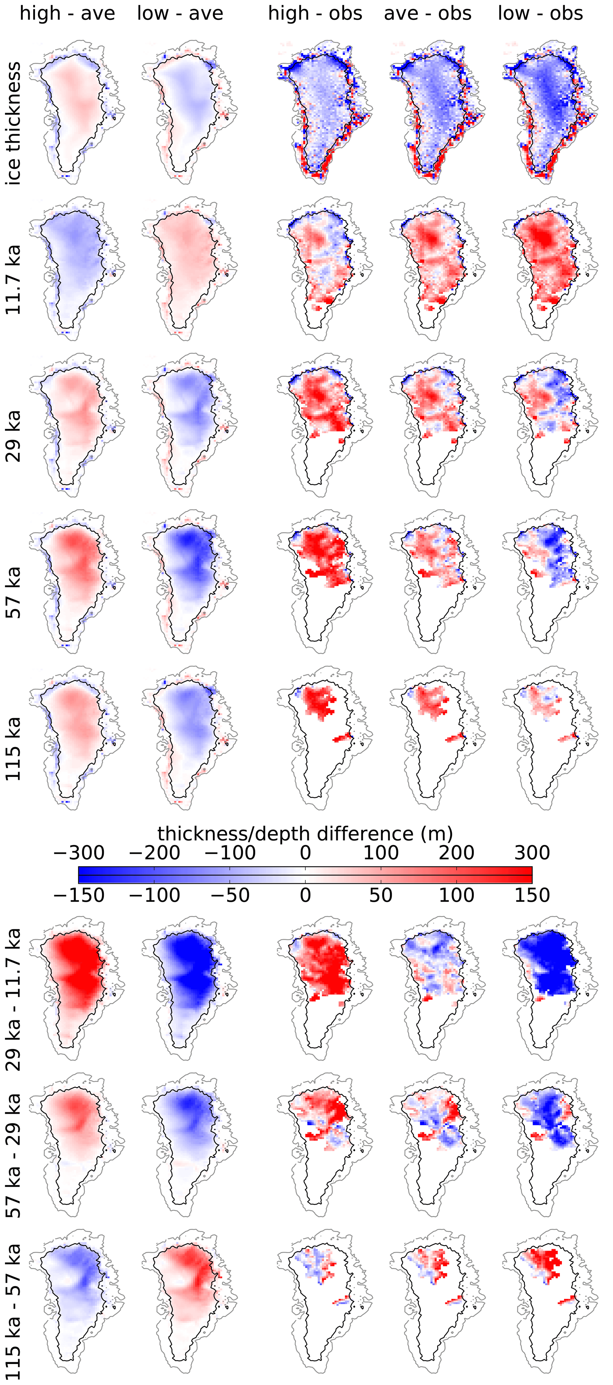
Figure A2 Like Fig. A1, but for composites of variable f_LGM. The ranges of the high and low composites are 1.5 to 2 and −2 to −1.5.