High-resolution topography of the Antarctic Peninsula combining the TanDEM-X DEM and Reference Elevation Model of Antarctica (REMA) mosaic

The Antarctic Peninsula (AP) is one of the widely studied polar regions because of its sensitivity to climate change and potential contribution of its glaciers to global sea level rise. Precise digital elevation models (DEMs) at a high spatial resolution are much demanded for investigating the complex glacier system of the AP at fine scales. However, the two most recent circum-Antarctic DEMs, the 12 m TanDEM-X DEM (TDM DEM) from bistatic interferometric synthetic aperture radar (InSAR) data acquired between 2013 and 2014 and the Reference Elevation Model of Antarctica mosaic (REMA mosaic) at an 8 m spatial resolution derived from optical data acquired between 2011 and 2017 have specific individual limitations in this area. The TDM DEM has the advantage of good data consistency and few data voids (approx. 0.85 %), but there exist residual systematic elevation errors such as phase-unwrapping errors in the non-edited DEM version. The REMA mosaic has high absolute vertical accuracy, but on the AP it suffers from extended areas with data voids (approx. 8 %). To generate a consistent, gapless and high-resolution topography product of the AP, we fill the data voids in the TDM DEM with newly processed TDM raw DEM data acquired in austral winters of 2013 and 2014 and detect and correct the residual systematic elevation errors (i.e., elevation biases) in the TDM DEM with the support of the accurately calibrated REMA mosaic. Instead of a pixelwise replacement with REMA mosaic elevations, these provide reference values to correct the TDM elevation biases over entire regions detected through a path propagation algorithm. The procedure is applied iteratively to gradually correct the errors in the TDM DEM from a large to small scale. The proposed method maintains the characteristics of an InSAR-generated DEM and is minimally influenced by temporal or penetration differences between the TDM DEM and REMA mosaic. The performance of the correction is evaluated with laser altimetry data from Operation IceBridge and ICESat-2 missions. The overall root mean square error (RMSE) of the corrected TDM DEM has been reduced from more than 30 m to about 10 m which together with the improved absolute elevation accuracy indicates comparable values to the REMA mosaic. The generated high-resolution DEM depicts the up-to-date topography of the AP in detail and can be widely used for interferometric applications as well as for glaciological studies on individual glaciers or at regional scales.

1 Introduction

Antarctic Peninsula (AP) glaciers (north of 70^∘ S) have the potential to raise the global sea level by 69±5 mm (Huss and Farinotti, 2014). In recent decades they have undergone extensive changes as a consequence of regional climate warming and oceanographic change (Cook et al., 2005, 2014, 2016; Seehaus et al., 2018; Rott et al., 2018; Rignot et al., 2019; Dryak and Enderlin, 2020). As a complex mountainous coastal glacier system, the mass balance of the individual glaciers is affected by climate and oceanographic forcings and also by the subglacial and surrounding topography (Cook et al., 2012). Digital elevation models (DEMs) are fundamental topographic data needed for investigating glacial features and monitoring glacier dynamics at individual glaciers or at regional scales. DEMs enable the delineation of drainage basins (Cook et al., 2014; Huber et al., 2017; Krieger et al., 2020a) and quantifying glacier mass balance with the geodetic method (Abdel Jaber et al., 2019; Krieger et al., 2020b; Rott et al., 2018; Helm et al., 2014). DEMs also support the mass budget method (Rignot et al., 2011b; Shepherd et al., 2018; Sutterley et al., 2014) and calculating ice velocity (Rignot et al., 2011a; Mouginot et al., 2012) and provide constraints for geodynamic and ice flow modeling (Cornford et al., 2015; Ritz et al., 2015).

The previously released DEMs of the AP mostly cover the whole Antarctic continent. They have been derived from satellite radar altimetry (Helm et al., 2014; Li et al., 2017; Slater et al., 2018), laser altimetry (DiMarzio et al., 2007), a combination of both radar and laser altimetry (Bamber et al., 2009; Griggs and Bamber, 2009), optical photogrammetry (ASTER GDEM Validation Team, 2009, 2011; Abrams et al., 2020; Howat et al., 2019), the combination of several sources of remote sensing and cartographic data (Liu et al., 2001; Fretwell et al., 2013), and single-pass synthetic aperture radar (SAR) interferometry of the TanDEM-X mission (German Aerospace Center DLR, 2018). In addition, regional DEMs of the marginal areas of the ice sheet have been generated from stereoscopic data (Korona et al., 2009; Fieber et al., 2018). An overview table with the parameters of the AP DEMs can be found in Table S1 of the Supplement. They reveal large elevation uncertainty, coarse resolutions, voids or incomplete data coverage over Antarctica and particularly over the AP because of the complex mountainous terrain and cloudy weather. To generate more accurate surface topography data of the AP, Cook et al. (2012) have created a DEM posted at 100 m by improving the ASTER GDEM datasets and smoothing the erroneous surface, but the 100 m grid size is still too coarse to analyze the glaciers' features and dynamics at fine scales. Similarly, the recently released circum-Antarctic DEM called TanDEM-X PolarDEM (Wessel et al., 2021) has some improvements (edits and filled voids) on the TanDEM-X global DEM but with 90 m posting is insufficient for the small-scale features present at the AP. There are numerous small outlet glaciers at the AP especially on the west coast; e.g., more than 400 glaciers have basin areas of less than 5 km². The high-resolution reference DEMs can facilitate some interferometric processing steps like the removal of the reference topographic phase for estimating ice velocity using the interferometric synthetic aperture radar (InSAR) technique (Mouginot et al., 2012) or single-pass InSAR DEM generation (Rott et al., 2018). Besides, the high-resolution topographic data can also be used for terrain feature calculation, e.g., slope, aspect or hypsometry, in a more detailed way (Cook et al., 2014). To meet the demand for high-resolution topography information, two DEM products have been recently released. One is the 12 m TanDEM-X global DEM (TDM DEM) based on InSAR data acquired over Antarctica between 2013 and 2014. The second is the 8 m Reference Elevation Model of Antarctica mosaic (REMA mosaic) derived from optical data acquired between 2011 and 2017 (Howat et al., 2019). The TDM DEM is characterized by good data consistency and few data voids (approx. 0.85 %), but there are residual systematic elevation errors caused by phase unwrapping (PU) in the non-edited version. The REMA mosaic has the advantage of high absolute vertical accuracy and an absence of regional outliers but has a larger number of data voids (approx. 8 %) and limited temporal consistency due to the relatively wide time span of images used to generate the DEM.

To obtain a consistent, gapless and precise DEM product at a high spatial resolution of the AP, these two up-to-date DEMs with comparable spatial resolutions have been combined. The main goal is to eliminate the PU errors in the TDM DEM which prevail over other error sources. Since REMA mosaic has high absolute vertical accuracy, the height difference map between these two DEM datasets can emphasize the residual PU errors as regional discrepant values with distinct boundaries with unaffected regions. To maintain the consistency of a DEM dataset in terms of acquisition time and the data source, we propose correcting the residual PU errors in the TDM DEM based on this elevation difference map. A novel multi-scale elevation bias detection and correction algorithm relying on a reference elevation surface is applied. The present method differs from existing DEM fusion techniques which usually combine the elevation information from different DEMs equally or by certain weights (Papasaika et al., 2009; Jiang et al., 2014; Gruber et al., 2016; Dong et al., 2018). Instead, adjacent pixels with similar elevation deviations from the real surface elevation can be automatically detected and merged into a common region and then corrected with an average vertical offset compensation value specific to each detected region. Since remaining elevation biases in the TDM DEM exist at different scales, the height offset correction is performed to gradually eliminate these errors from large to small scales. The elevation accuracy of the resulting DEM was validated with laser altimetry data to illustrate the effectiveness of the proposed algorithm.

2 Experimental area and data

2.1 Experimental area

The Antarctic Peninsula (AP) between 63 and 70^∘ S (Fig. 1), belonging to Graham Land, is a long coastal area along the Weddell Sea on the east side and the Bellingshausen Sea on the west side. Based on the newest glacier inventory of the AP of Cook et al. (2014) and Huber et al. (2017), there are 860 marine-terminating glaciers out of 1590 glacier basins. It has complex mountainous terrain with elevations rising steeply from sea level at the coast towards snow-covered flat plateaus located above 1500 m. The highest peaks are close to 3000 m a.s.l. The outlet glaciers and cirques lie at lower altitudes and flow into ice shelves or terminate as grounded or floating tidewater glaciers. Their accumulation areas connect with the plateaus directly or through the escarpments with steep slopes.

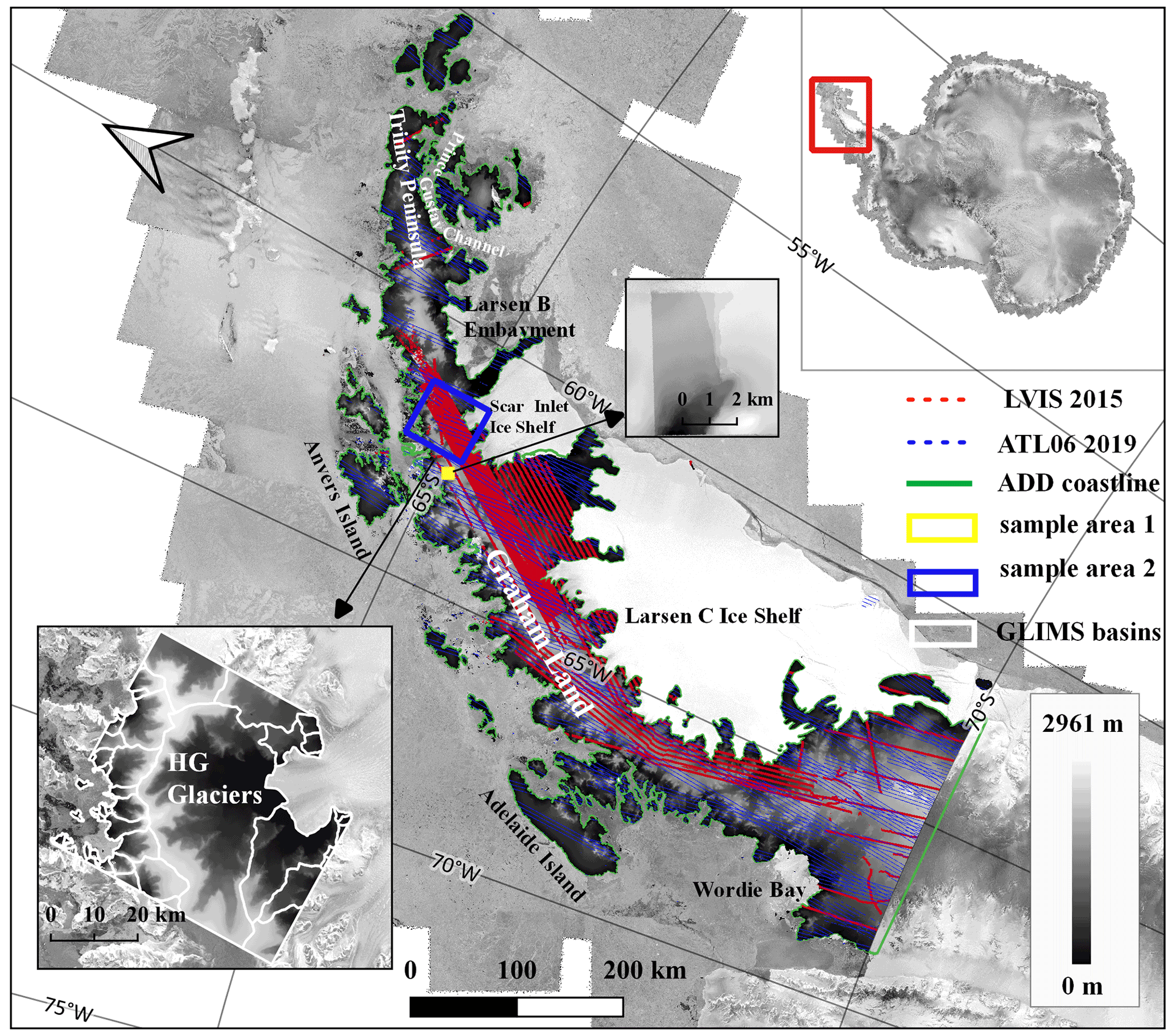
Figure 1 Experimental area and TanDEM-X DEM coverage over the Antarctic Peninsula. Dotted red and blue lines: the footprints of the LVIS 2015 and ATL06 2019 laser points, respectively. Green outline: the coastline mask from the Antarctic Digital Database (ADD). Blue and yellow boxes: sample areas of the experimental results corresponding to the two zoomed-in windows. White outline: glacier basins from GLIMS around Hektoria and Green (HG) glaciers. Background: RADARSAT-1 Antarctic Mapping Project (RAMP) imagery mosaic (Jezek, 1999; Jezek et al., 2013) from Quantarctica (Matsuoka et al., 2021).

2.2 Experimental data

2.2.1 TanDEM-X DEM (TDM DEM)

The German TanDEM-X (TerraSAR-X add-on for digital elevation measurements) mission is a bistatic SAR interferometer built by two almost identical satellites (TerraSAR-X and TanDEM-X) flying in close formation (Krieger et al., 2007, 2013). The advantage of the single-pass SAR interferometer is to acquire highly coherent cross-track interferograms, which are not affected by temporal decorrelation and atmospheric phase delay. Besides, the TDM DEM is unaffected by the cloud cover or varying solar illumination conditions, which is the main reason for the completeness of the TDM DEM. The primary objective of the TanDEM-X mission was the generation of a worldwide, consistent, timely and high-precision DEM as the basis for a wide range of scientific research. The resulting main product, the TDM DEM, has a nominal pixel spacing in the latitude direction of 0.4 arcsec, corresponding to approximately 12 m at the Equator. The obtained overall absolute vertical accuracy at a 90 % confidence level is just 3.49 m, and in areas covered with ice and snow like Greenland and Antarctica the obtained absolute vertical accuracy is about 6.37 m (Rizzoli et al., 2017a). The TDM DEM is also available with a pixel spacing of 1 and 3 arcsec (Wessel, 2016), but in our study over the AP, we focus on the nominal product at about a 12 m cell size. The elevation values represent the ellipsoidal elevations relative to the WGS 84 ellipsoid in the geographic coordinate system.

The bistatic InSAR data used for generating the TDM DEM over Antarctica were acquired during two dedicated campaigns lasting from April to November of 2013 and 2014. The concentration of the acquisition time over Antarctica reduces the temporal changes in the terrain surface and thus guarantees the consistency of the TDM DEM product. The TanDEM-X mission has acquired multi-coverage of Antarctica from different orbital directions and height ambiguities in order to compensate for geometric distortions (Gruber et al., 2016) and improve phase unwrapping with the dual-baseline phase-unwrapping algorithm (Lachaise et al., 2018). However, due to the complicated mountainous terrain conditions of the AP, there still exist elevation biases caused by phase-unwrapping errors and geometric distortions in the non-edited TDM DEM, which contaminate the vertical accuracy of the TDM DEM. Besides the elevation offset, a horizontal shift because of calibration errors will also propagate into the final DEM product due to the mosaicking process.

2.2.2 The Reference Elevation Model of Antarctica (REMA) mosaic

The REMA DEM was generated from stereophotogrammetry with high-resolution optical, commercial satellite imagery and covers nearly 95 % of the whole of Antarctica. Unlike other common stereo-capable imagers such as the Advanced Spaceborne Thermal Emission and Reflection Radiometer (ASTER), the optical imagery used for generating REMA is of a high spatial and radiometric resolution, which ensures accurate measurements over low-contrast ice sheet surfaces (Howat et al., 2019).

The REMA mosaic at an 8 m resolution used in this paper was provided in 100×100 km² tiles and mosaicked from the individual time-stamped DEM strips which were quality-controlled and vertically registered (Howat et al., 2019). The absolute vertical accuracy of the REMA strips and mosaic products is less than 1 m based on validation with data acquired by three NASA Operation IceBridge (OIB) airborne lidar instruments: the Airborne Topographic Mapper (ATM); the Land, Vegetation, and Ice Sensor (LVIS); and the ICECAP laser altimeter system (Howat et al., 2019). Considering the data acquisition efficiency and the effects of cloud cover and varying illumination, a limitation of the REMA mosaic is that the time span of stereo image acquisition to generate the REMA mosaic lasted for 7 years from 2011 to 2017, and the data voids in the final DEM mosaic at the AP are visible in Fig. S1 in the Supplement and are estimated to amount to approximately 8 % of the AP's landmass area based on our statistics.

The REMA mosaic is referenced to WGS 84 ellipsoid and in polar stereographic projection with a central meridian of 0^∘ and standard latitude of −71^∘ S. For the present paper, we converted the REMA mosaic Release 1.1 to the geographic coordinate system with the same grid size as the TDM DEM.

2.2.3 Laser altimetry data

In order to evaluate the vertical accuracy of the TDM DEM before and after automatic correction, we use the airborne laser altimetry data over Antarctica acquired by NASA OIB. In Fig. 1 we selected the LVIS Level-2 geocoded elevation product acquired in September and October 2015 for its dense coverage in the central part of the AP (Blair and Hofton, 2019). The absolute vertical accuracy of LVIS is about 0.1 m, and the footprint size is about 20–25 m (Hofton et al., 2008).

To obtain a complete evaluation of the whole experimental area, we also use the evenly distributed Level-3A geocoded land ice height dataset ATL06 acquired in the austral winter of 2019 by the Advanced Topographic Laser Altimeter System (ATLAS) instrument of the ICESat-2 satellite mission (Smith et al., 2019). The ATL06 footprint is about 17 m in diameter, and the surface elevation measurement accuracy is better than 0.1 m (Brunt et al., 2019). The coverage of ATL06 data is shown in Fig. 1. For simplicity of the presentation, the two laser altimetry datasets used as validation data are abbreviated as LVIS 2015 and ATL06 2019.

2.2.4 Coastline mask

In order to improve the calculation efficiency, we use the coastline mask from the Antarctic Digital Database (ADD) (https://add.data.bas.ac.uk/, last access: 13 February 2020) which is marked by the green outline in Fig. 1. The current version 7.1 was last updated in August 2019. We have visually checked the agreement between the ADD coastline product and hillshade map of the TDM DEM at the AP and found most of the glacier fronts are contained within or agree with the ADD coastline.

3 Methodology

We propose a novel method to detect and correct the residual systematic elevation errors (referred to as elevation biases) in the 12 m TDM DEM facilitated by the REMA 8 m mosaic tiles. The detailed methodologies are organized into four modules (Fig. 2). Firstly, we analyzed the characteristics of the residual multi-scale elevation errors in the TDM DEM with the REMA mosaic as ground reference. Secondly, we developed a path propagation algorithm to automatically detect the erroneous regions with elevation biases based on the scales of elevation errors and spatial adjacency. Thirdly, instead of replacing the erroneous elevation values with the corresponding REMA mosaic, we selected stable points from the buffer zone of the erroneous region in TDM DEM to fit a reference elevation surface and then calculate the compensation offset to the fitted elevation surface. Fourth, the above detection and correction procedure is iteratively performed to correct multi-scale elevation errors. Details of each module are given in the following sections.

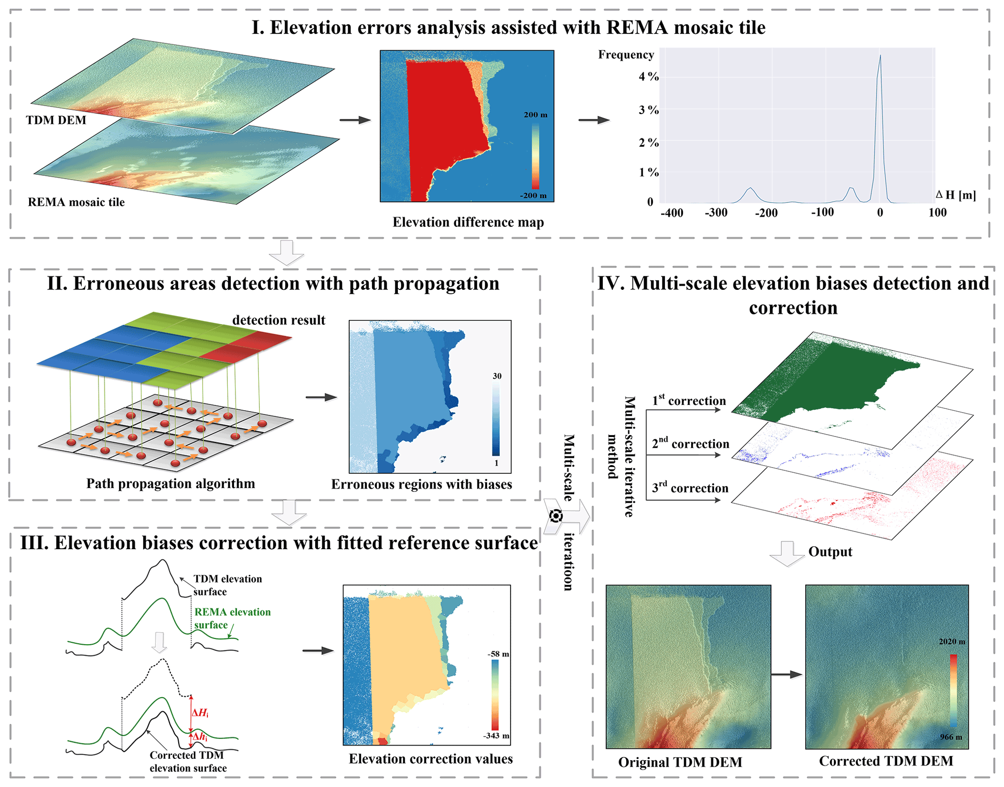
Figure 2 The framework of TDM DEM correction with REMA mosaic tiles organized in modules I to IV.

3.1 TDM DEM elevation error analysis assisted by REMA mosaic

The remaining elevation errors in the TDM DEM include the random errors introduced from the phase noise and the systematic errors caused by the baseline calibration errors, geometric distortions such as layover and shadow, and phase-unwrapping (PU) errors. Details on each of these elevation errors are given below.

1. Random elevation errors. The random or theoretical error in the TDM DEM is linearly related to the interferometric phase error which in turn depends on the coherence and baseline geometry and slightly increases from near to far ranges (Rizzoli et al., 2012, 2017a). A height error map (HEM) accompanies each TDM DEM tile, representing a combined estimate of the corresponding random elevation errors σ_ran from the interferometric coherence and acquisition geometry (Wessel, 2016). The TDM DEM is formed by a weighted average of DEMs acquired from multiple coverages to reduce the aforementioned random errors. The relative vertical accuracy which accounts for random errors only is reported as 2.72 and 2.41 m at the 90 % confidence level for flat and steep terrain of Antarctica and Greenland (Rizzoli et al., 2017a). However, this relative vertical accuracy specification of the TDM DEM is a global statistic and local performance could be degraded due to the presence of confined local outliers (Rizzoli et al., 2017a).

2. Elevation errors from baseline calibration. The TDM DEM has gone through a sophisticated calibration process to improve the baseline accuracy, including instrument and baseline calibration (González et al., 2012). The correction of residual offsets and tilts in the azimuth and range is performed by means of a least-squares block adjustment with ICESat laser altimetry data (Gruber et al., 2012). The final baseline accuracy is on the order of 1 mm for a ground extension of about 30 km×50 km, which corresponds to a vertical offset on the order of 1 m (Rizzoli et al., 2017a). A vertical offset is always accompanied by a tilt and a shift in the range direction for DEM scenes. When combining the DEM scenes together into the final mosaic, the vertical offsets and horizontal shifts are likely to cause elevation biases or a block-shaped elevation anomaly when there are residual phase-unwrapping errors.

3. Elevation errors from geometric distortions. At the high-relief terrain, the DEM quality is reduced due to the geometric distortions such as the layover or shadow. The erroneous regions affected by the geometric distortions can be data voids or outliers. These kinds of elevation error are usually compensated for by the fusion of ascending and descending DEM acquisitions. For the TanDEM-X mission, the landmass was mapped at least twice with complementary imaging geometries, the acquired DEMs were screened, and the non-discrepant data were grouped and then weighted and averaged to generate the final TDM DEM, which can effectively fill in most data gaps caused by layover or shadow (Gruber et al., 2016). The remaining elevation errors due to geometric distortions are small in spatial extent and sparsely distributed over the steep slopes oriented towards the radar or away from it.

4. Elevation errors from phase-unwrapping errors. The phase unwrapping (PU) is a crucial step in interferometric applications and hence also in the surface elevation retrieval. It is very difficult to achieve an error-free PU at the AP because the complex mountainous terrain is prone to cause dense fringes and phase jumps. The phase-unwrapping errors possibly exist in single TDM DEM acquisitions (TDM raw DEMs). Elevation differences between single TDM DEM acquisitions (TDM raw DEMs) accounting for PU errors are on the order of an integer multiple of the height of ambiguity (HoA). The HoA is the height that corresponds to one phase cycle after phase-to-height conversion and is typically in the range of 30 to 80 m for most of the twin satellite baseline configurations during the nominal TanDEM-X acquisitions. Gruber et al. (2016) estimated the minimum elevation difference dp_PUthres between TDM raw DEMs introduced by phase-unwrapping errors as dp${}_{\mathrm{PUthres}}=\mathrm{0.75}\cdot min\left(\right|\text{HoA}\left|\right)-\mathrm{4}$ [m] considering the random elevation errors and the possible residual calibration inaccuracies (within 4 m). In our study, we detect the residual systematic elevation errors in the TDM global DEM through calculating the elevation difference map ΔH with the REMA mosaic. The minimum elevation difference ΔH_PUthres due to phase-unwrapping errors in the TDM DEM is empirically adjusted to Eq. (1). The first item in the right part of Eq. (1) is reduced to $\mathrm{0.6}\cdot min\left(\right|\text{HoA}\left|\right)$ [m] compared to the estimation of Gruber et al. (2016) because the AP is a mountainous area with snow and ice cover which causes higher random-elevation noise for both the TDM DEM and REMA mosaic. ΔH_PUthres is then reduced by 1 m considering the calibration error in the TDM global DEM is at about 1 m (Rizzoli et al., 2017a). Since the minimum HoA of the TanDEM-X mission is about 30 m, the minimum elevation difference to detect an inconsistency introduced by a PU error is approximately 17 m based on Eq. (1).

   $$\begin{array}{}\text{(1)}& \mathrm{\Delta }{H}_{\mathrm{PUthres}}=\mathrm{0.6}\cdot min\left(\left|\text{HoA}\right|\right)-\mathrm{1}\end{array}$$

Based on the above analysis, it can be seen that the remaining elevation errors in the TDM DEM causing large inconsistencies are mainly introduced by the systematic elevation errors especially the PU errors. Therefore, we propose detecting and correcting the remaining systematic elevation errors in the TDM DEM with the REMA mosaic as the reference DEM. Figure 3a shows a sample area with PU error in the TDM DEM, which is also visible as an elevation jump in the TDM DEM elevation profile crossing the boundary of the inconsistent region (Fig. 3d) as well as a large discrepancy in the elevation difference map between the TDM DEM and REMA mosaic (blue region in Fig. 3c). In the elevation difference histogram (Fig. 3e), the remaining elevation biases can be identified as side lobes adjoining the main lobe near zero. This abnormal elevation jump distinguishes the PU errors from the temporal change in elevation or penetration depth which are transitional changes with a certain trend. In other words, the elevation errors in the TDM DEM caused by PU errors are characterized by local elevation discrepancies with abrupt elevation jumps at the boundary where they occur. Elevation errors caused by the geometric distortions such as layover or shadow also exist on rugged terrain. They have more variations in smaller spatial sizes compared to the phase-unwrapping errors. In the following sections (Sect. 3.2 to 3.4), we are using the characteristics of the remaining elevation biases to detect and correct these large discrepancies present in the TDM DEM.

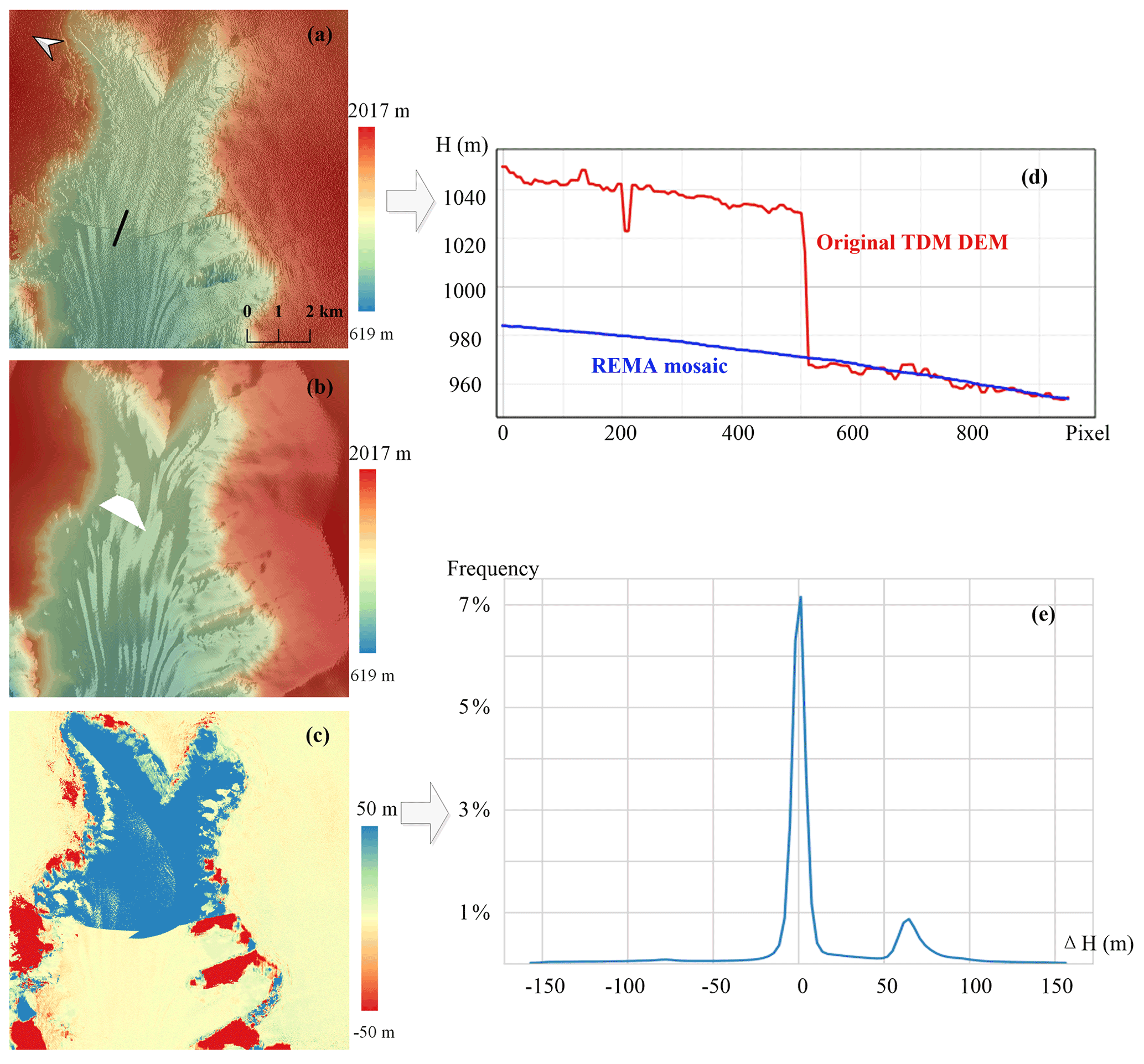
Figure 3 Sample area with residual phase-unwrapping elevation errors. (a) TDM DEM. (b) REMA mosaic with data void in white. (c) Elevation difference map between TDM DEM and REMA mosaic. (d) Elevation profile corresponding to the black line in (a). (e) Histogram of the elevation difference map.

3.2 Erroneous area detection with path propagation algorithm

The automatic detection of the areas with elevation errors from the elevation difference map between the TDM DEM and REMA mosaic is performed with a novel path propagation algorithm where neighboring pixels with similar local elevation offset values are detected and merged into one region. Compared with the commonly used connected-component labeling method implemented in famous image processing libraries (such as the scikit-image library) for binary images, the path propagation is generally a region extraction algorithm and takes the elevation difference as the input. The algorithm gradually merges and labels each adjacent target point with similar local elevation offsets along the searched path to form a correction area. An example of erroneous area detection with a path propagation algorithm is illustrated in Fig. 4. The elevation difference value in meters for each pixel used as input is shown in Fig. 4a. The pixels can be divided into background and target pixels based on their corresponding elevation difference values. The background pixels (in grey in Fig. 4b and c) have elevation differences below a threshold value and will not be corrected in the following process. The remaining pixels are regarded as target pixels to be processed (light orange pixels in Fig. 4b). The main task is to merge spatially adjacent target pixels with similar local elevation offsets into common regions. Then each of these regions can be corrected individually by the compensation value of the corresponding region. With the path propagation method, the target pixels will search their four- or eight-neighborhood direction for homogeneous pixels. For simplicity of explanation in Fig. 4b only the four-neighborhood search is shown. The similarity criterion between the adjacent target pixels i and j is the absolute difference in their elevations (H):

$$\begin{array}{}\text{(2)}& \left|H_i-H_{j\in N_i}\right|\le T_{\mathrm{\Delta }H},\end{array}$$

where T_ΔH is the given threshold and N_i represents the neighborhood of pixel i. If the similarity criterion in Eq. (2) is fulfilled, the corresponding neighboring target pixels will be merged into the same region.

The newly added target pixels will continue searching their neighboring target pixels. To correctly compensate for the mean elevation offset of the erroneous region, it is important to detect the regions with a homogeneous offset accurately. The existence of background pixels improves the calculation efficiency and most importantly cuts off the propagation path of target pixels. Furthermore, it is very important to properly inhibit the propagation path of target pixels not only with the background pixels but also based on the dissimilarity between the neighboring target pixels. In our example we set T_ΔH=7 m for the neighboring pixels, and pixels along the propagation path (marked with green arrows in Fig. 4b) can be merged into one region. The propagation path stops at pixels with an absolute elevation difference larger than T_ΔH as well as at the background pixels. Finally, the target pixels are merged into two separate regions according to the similarity of the elevation offsets (Fig. 4c).

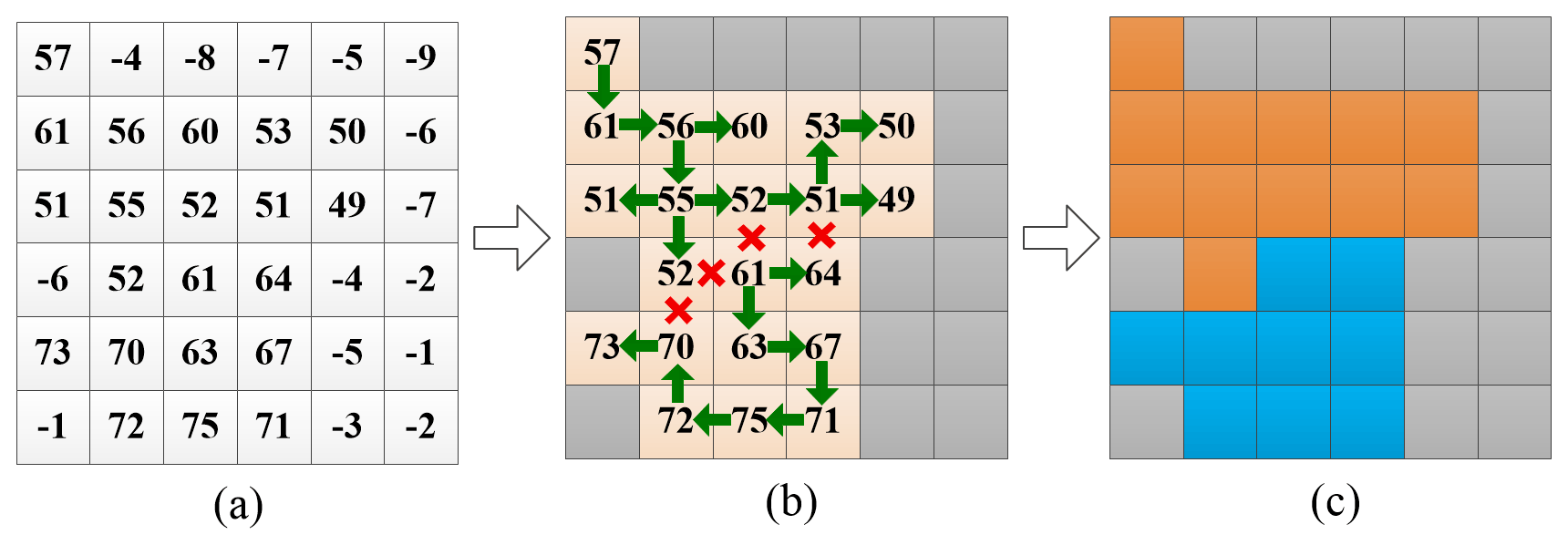
Figure 4 Erroneous area detection with a path propagation algorithm. (a) TDM DEM − REMA elevation difference values in meters. (b) Elevation jump detection with path propagation. Green arrows and red crosses represent the adjacent pixels which can and cannot, respectively, be merged along the propagation path. Grey: background pixels. (c) Resulting automatically merged regions in orange and blue with mean elevation difference of 53.9 and 68.4 m, respectively.

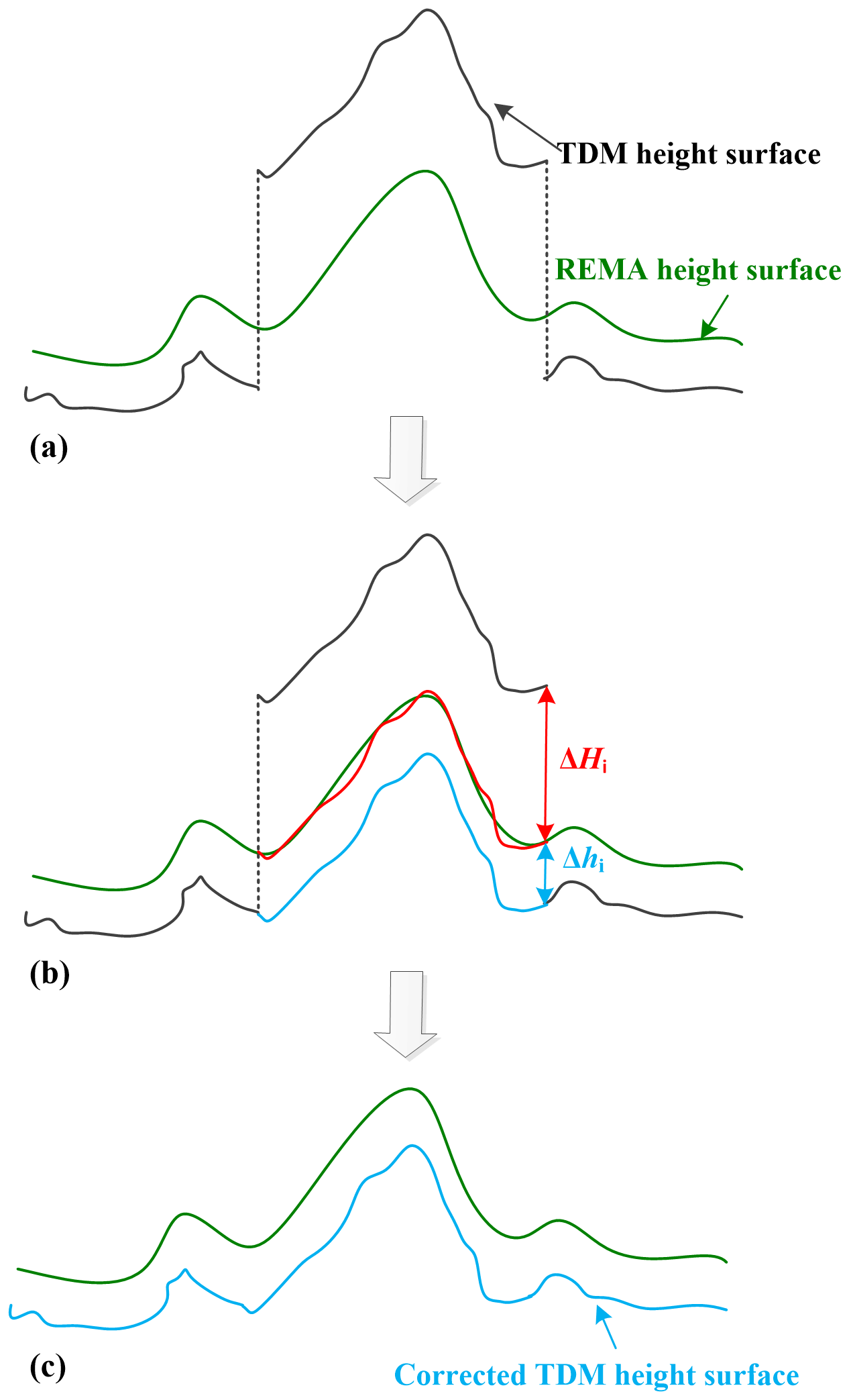
Figure 5 Schematic representation of the local elevation offset correction procedure. (a) Erroneous elevation jump of the TDM DEM and the REMA surface elevation, (b) Correction of the jump with fitted elevation surface as in Eq. (3). Red: corrected elevation surface with mean offset. Blue: corrected elevation surface with additional fitted elevation surface. (c) Finally corrected TDM DEM.

3.3 Elevation bias correction based on fitted reference surface

After merging the targeting pixels with similar local elevation offsets into regions, the elevation error correction of the TDM DEM based on the REMA mosaic taken as reference is performed for each of these regions. Taking the differences due to the SAR signal penetration depth into snow and firn and to possible temporal elevation changes between the TDM DEM and REMA mosaic into consideration, we do not simply correct the TDM DEM to the reference elevation surface of REMA mosaic directly. Instead, we create a buffer zone around each corrected region. Stable points whose elevation difference with the REMA mosaic is less than a given threshold value are extracted from the buffer zone. The average elevation surface fitted from these selected stable points is used as a reference elevation surface for elevation offset correction. As shown in Fig. 5 the correction elevation value $\mathrm{\Delta }{\widehat{H}}_{\mathrm{corr},i}$ for each region i can be calculated as the sum of the average elevation difference between the REMA mosaic and TDM DEM, ΔH_i, and the mean elevation difference in selected stable points inside the buffer zone, Δh_i:

$$\begin{array}{}\text{(3)}& \mathrm{\Delta }{\widehat{H}}_{\mathrm{corr},i}=\mathrm{\Delta }{H}_i+\mathrm{\Delta }{h}_i.\end{array}$$

3.4 Multi-scale corrections of elevation errors in the TDM DEM

Since the residual elevation errors in the TDM DEM may have a wide range of values, the histogram of the TDM DEM elevation errors (quantified as differences to REMA mosaic elevations) usually has several side lobes adjoining the main zero-centered lobe as illustrated in the first module of Figs. 2 and 3e. Actually, additional smaller side lobes within the non-zero peaks are likely. Consequently, the segmentation results of the erroneous regions from the path propagation algorithm may also contain pixels with elevation offsets at different scales. Thus, the inhomogeneous region cannot be accurately corrected just with a single mean offset value.

To compensate for the remaining elevation errors in the TDM DEM more accurately, we propose adopting a multi-scale correction method to gradually correct the elevation errors from large to medium and small scales. As described in Sect. 3.2 the path propagation algorithm is only performed among pixels with an elevation difference larger than a certain threshold; all other pixels are labeled as background pixels. For each correction, the background pixels which do not need to be corrected are set based on the threshold that determines different scales of elevation biases. In order to achieve accurate segmentation results of the elevation inconsistency regions, the path propagation should be effectively cut off at the boundaries between different erroneous regions. The large-scale elevation errors have a clear boundary in the elevation difference map and can be more easily detected and corrected. Therefore, the multi-scale correction method starts with the large-scale elevation errors by setting an empirically determined threshold on the TDM DEM-to-REMA mosaic elevation difference. In this step all the pixels with an elevation difference less than the threshold are marked as background, and no correction is applied. After this first iteration of large-scale elevation error correction, the number of background and stable points needed for the following medium-scale or small-scale correction steps increases and the propagation path for target pixel merging can be well restricted and cut off. Hence, the homogeneity degree of the merged regions in terms of elevation errors increases accordingly. Similarly, the medium- or small-scale elevation errors are successively corrected to obtain a high-precision corrected DEM. In our experiments, we empirically set the elevation thresholds for the multi-scale correction as the large-scale errors (>45 m), medium-scale elevation errors (>20 m) and the small-scale elevation errors (>5 m). Examples of how the multi-scale correction is applied are shown in Sect. 5.2.

4 Experiments

In order to test the effectiveness of the proposed algorithm at different spatial scales, we applied our methodology to a series of sample areas. Their spatial extent increased from the local, about an 11 km×11 km large area, to the glacier scale (yellow and blue rectangles in Fig. 1, respectively) and finally covered the entire Antarctic Peninsula. The voids visible in the 8 m REMA mosaic tiles were filled with the oversampled 100 m REMA mosaic tiles, leading to a gapless reference elevation map. To generate the elevation difference map, the REMA mosaic was resampled into the same grid size as the TDM DEM.

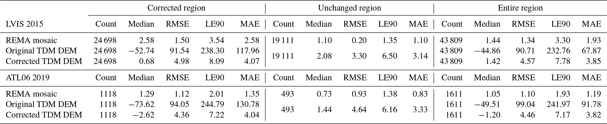
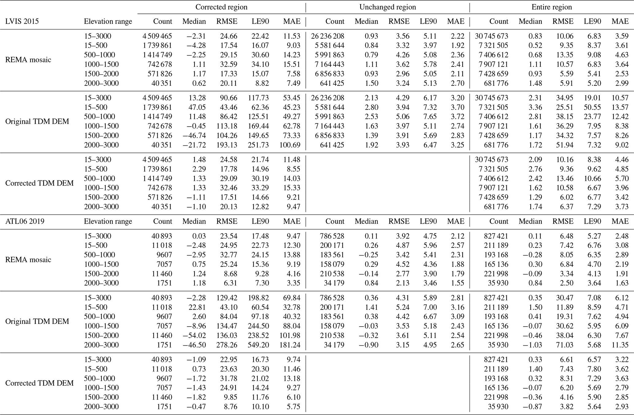
For quantitative accuracy evaluation of different DEM datasets, the laser altimetry datasets LVIS 2015 and ATL06 2019 described in Sect. 2.2.3 were used as ground reference. Differences between the laser altimetry points and the corresponding DEM elevation values obtained by bilinear interpolation were calculated. To show the vertical accuracy of different elevation intervals, we partitioned the laser points based on the elevation ranges. To compensate for the temporal differences between the laser points and the DEM datasets, we incorporated the large-scale elevation change maps from Smith et al. (2020). The annual surface elevation change was converted to elevation change by multiplying by the acquisition time span between the DEMs and laser altimetry points. At the footprints of the ATL06 2019 laser points used for evaluation, the statistics of the temporal elevation corrections are −0.7 m (mean), −2.4 m (10 % quantile) and 0.7 m (90 % quantile) for the REMA DEM and −1.1 m (mean), −4.8 m (10 % quantile) and 0.8 m (90 % quantile) for the TDM DEM. At the footprints of the LVIS 2015 laser points used for evaluation, the corresponding statistics are −0.4 m (mean), −1.2 m (10 % quantile) and 0.6 m (90 % quantile) for the REMA DEM and −0.6 m (mean), −3.2 m (10 % quantile) and 0.3 m (90 % quantile) for the TDM DEM.

The temporal elevation change is compensated for by the elevation difference between the DEMs and laser points before calculating the error statistics. To evaluate the elevation accuracy of the DEM datasets objectively and robustly from the outliers, we selected four typical error statistics: the median error (median), root mean square error (RMSE), the 90 % quantile of the absolute value of the elevation errors (which is also called the 90th-percentile linear error, LE90) and the mean average error (MAE). To better verify the effectiveness of the proposed correction algorithm, the error statistics were calculated independently for the corrected regions (before and after correction) and the ones left unchanged.

4.1 Experimental results in a local area

When comparing the original TDM DEM and the corresponding REMA mosaic (Fig. 6a and b, respectively), elevation surface offsets with boundaries caused by phase unwrapping and DEM calibration errors are visible in the TDM DEM as well as in the elevation difference map (Fig. 6c). We applied the proposed multi-scale correction algorithm to calculate the correction values (Fig. 6d) based on the elevation difference map. Finally, the corrected TDM DEM (Fig. 6e) results in a smooth elevation surface after successfully removing the elevation offsets. The elevation difference map between the corrected TDM DEM and REMA mosaic (Fig. 6f) shows a more consistent trend around zero with the elevation difference range reducing from ±200 to ±50 m.

The DEM elevation errors at each LVIS and ATL06 point shown in Fig. 6a were calculated, and the error statistics are shown in Table 1. Considering the elevation range of the laser altimetry points located in this sample area, we merely calculate the statistics from 1500 to 2000 m. For the REMA mosaic, the RMSE is less than 2 m and the MAE is no more than 3 m for both LVIS 2015 and ATL06 datasets in both corrected and uncorrected regions, indicating that the REMA mosaic is high precision and qualified as ground reference for TDM DEM elevation error correction. For the corrected TDM DEM in the corrected region, all the error statistics reduce considerably compared to the original TDM DEM. Specifically, the RMSE has decreased from larger than 90 m to less than 5 m and the MAE has decreased from larger than 110 m to less than 5 m in the corrected regions of the TDM DEM for both the LVIS 2015 and ATL06 datasets.

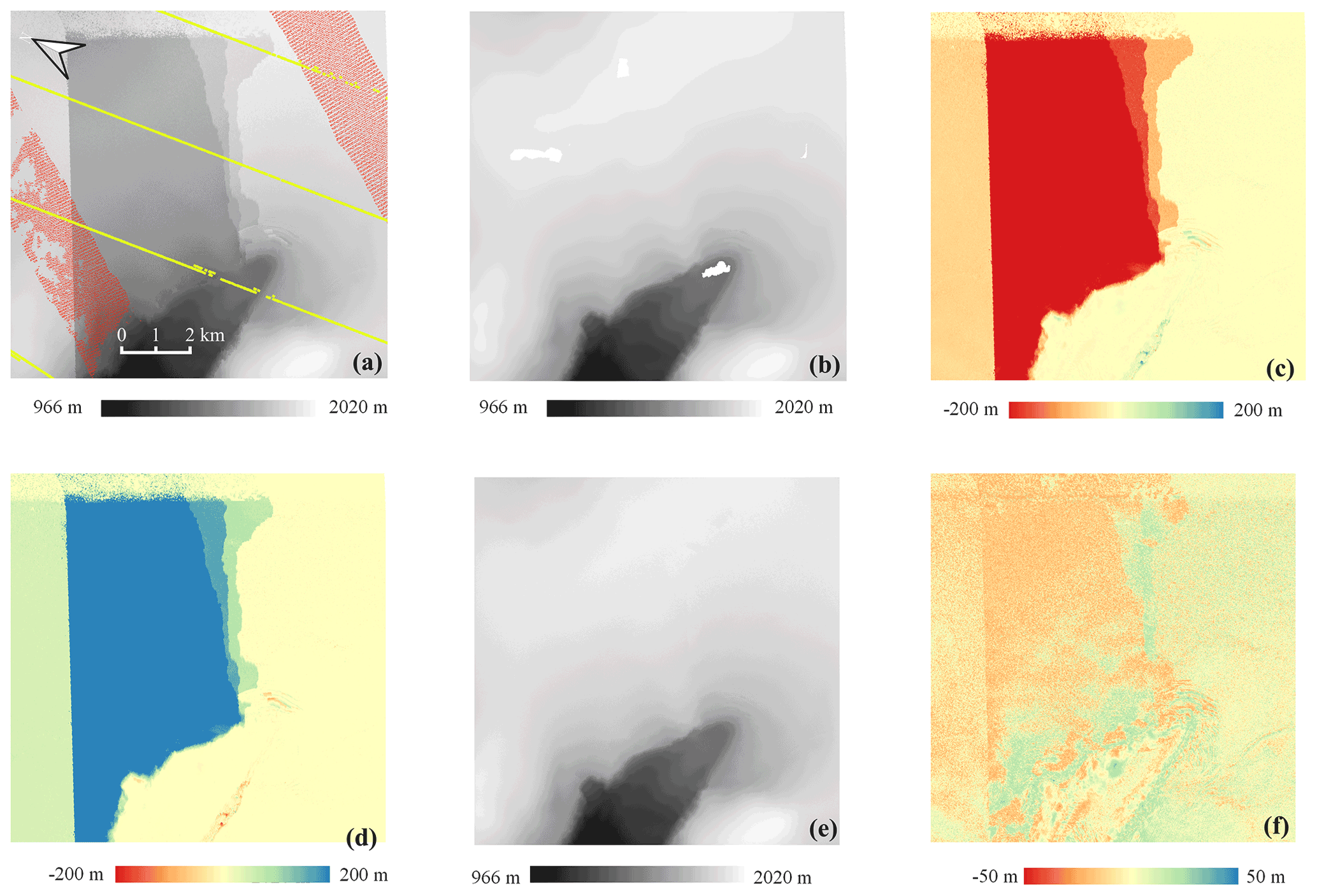
Figure 6 Experimental results in a local 11×11 km² sample area. (a) Original TDM DEM. Red and yellow: the footprints of LVIS 2015 and ATL06 2019. (b) Original REMA mosaic elevations with unfilled voids. (c) Elevation difference: TDM DEM minus REMA mosaic. (d) Correction map as obtained with Eq. (3). (e) Corrected TDM DEM. (f) Residual elevation difference: corrected TDM DEM minus REMA mosaic.

Table 1 Statistics of DEM elevation differences between the laser points and the REMA mosaic and the original and corrected TDM DEMs over the local sample area in Fig. 6. The elevation range is 1500–2000 m. All elevation units are in meters. Elevation difference: DEM elevation minus laser elevation. We separately considered the statistics for points affected by elevation biases where correction was applied and those falling into unchanged areas.

4.2 Experimental results on Hektoria and Green glaciers

For testing of our method at the glacier scale, we selected an area of about 55 km×60 km covering the Hektoria and Green (HG) glaciers, two adjacent outlets on the eastern AP. The elevation difference map between the original TDM DEM and the void-filled REMA mosaic (Fig. 7c) clearly shows regions with elevation errors of tens of meters in the TDM DEM. After applying the same methodology demonstrated for the local experimental area (Sect. 4.1), the erroneous regions are considerably reduced as revealed by the elevation difference map between the corrected TDM DEM and REMA mosaic (Fig. 7f).

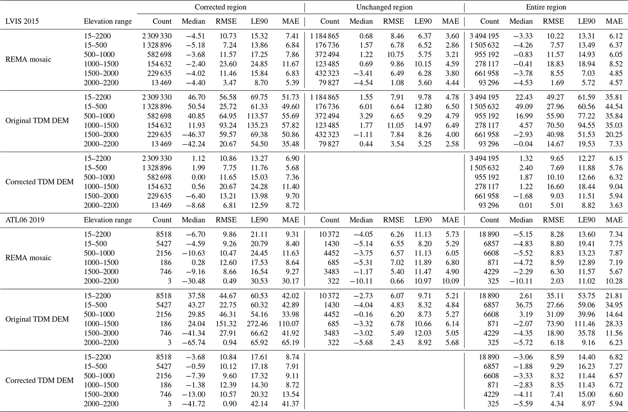
The laser altimetry point measurements (coverage shown in Fig. 7a) were used to validate our correction over the HG area. We divided the elevation range of the scene (18 to 2150 m) into five intervals for which we calculated the corresponding statistics of the elevation differences between the TDM and laser elevations (Table 2). There are about 3.5×10⁶ laser altimetry points of the LVIS 2015 dataset for validation, while there are only about 1.9×10⁴ points of the ATL06 2019 dataset. The variety in number of points can partly explain for the differences between error statistics. For example there are only 3 points of ATL06 2019 at the elevation interval ge2000 m, indicating that the corresponding statistics are less trustworthy than those of the LVIS 2015 dataset with 13 469 points. The steep escarpment, dropping abruptly about 500 m in elevation from 1500 to 1000 m a.s.l., generates layover and shadow in the SAR image and occlusion in the optical image and contributes to the high elevation errors of DEMs in this interval (Rott et al., 2018). From a glaciological standpoint, the most dynamic areas are the outlet glaciers mainly located below 1000 m a.s.l., whereas the flat firn plateaus stretch above 1500 m a.s.l. and have relatively stable surface elevation (Rott et al., 2018). In Table 2, the error statistics are comparable for the elevation range ≤1000 and ≥1500 m for both the REMA mosaic and corrected TDM DEM, indicating that the influence of the temporal surface elevation change is compensated for in error statistics due to the temporal change compensation. For the corrected region in Table 2, all the error statistics have been reduced significantly. The MAE and RMSE of the original TDM DEM larger than 50 m for the LVIS 2015 and larger than 40 m for the ATL06 2019 datasets have been reduced to about 10 and 8 m, respectively, for both validation datasets. The original TDM DEM in the unaltered region, the corrected TDM DEM and the REMA mosaic have comparable elevation accuracies based on the error statistics. The effectiveness of the proposed multi-scale elevation bias correction method is validated both qualitatively and quantitatively at the individual glacier scale.

Figure 7 Experimental results of Hektoria and Green (HG) glaciers. (a) Original TDM DEM. Red and yellow: the footprint of LVIS 2015 and ATL06 2019, respectively. (b) Original REMA mosaic with voids. (c) Elevation difference: TDM DEM minus REMA mosaic. (d) Correction map for the TDM DEM. (e) Corrected TDM DEM. (f) Residual elevation difference: corrected TDM DEM minus REMA mosaic.

Table 2 Statistics of DEM elevation differences between the laser altimetry points and REMA mosaic and the original and corrected TDM DEMs over the Hektoria and Green glacier area in Fig. 7. All elevation units are in meters. Elevation difference: DEM elevation minus laser elevation. We separately considered the statistics for points affected by elevation biases where correction was applied and those falling into unchanged areas.

4.3 Experimental results on the Antarctic Peninsula

The multi-scale elevation error correction was also applied to the entire Antarctic Peninsula north of 70^∘ S (Fig. 8 left) covering about 95 000 km². Because the corrections are not visible over such a large area, we show the results in the detailed views of three sample areas marked as A, B and C (Fig. 8a1–c2). Within each area, the corrected elevations become smooth and continuous with elevation jumps successfully eliminated. The corrected TDM DEM was evaluated with the LVIS 2015 and ATL06 2019 datasets covering the entire AP according to the footprints shown in Fig. 1. The statistics of the DEM elevation errors at the laser points are presented in Table 3. There are about 3.1×10⁷ and 0.8×10⁶ laser points of the LVIS 2015 and ATL06 2019 datasets, respectively, which are enough validation points to verify the elevation accuracy of the DEM datasets. In terms of the whole experimental area, the RMSEs of the plateaus above 1500 m are the smallest because of the flat topography, while the RMSEs of the elevation intervals between 500 and 1500 m are larger due to the existence of the escarpments. The elevation errors of the corrected region of the TDM DEM decrease clearly after the PU error correction. The RMSEs have reduced from about 100 to 20 m and MAEs have decreased from about 60 to 10 m for the LVIS 2015 and ATL06 2019 datasets. In the unaltered region, the RMSEs and MAEs are all less than 5 m for the TDM DEM and REMA mosaic for both LVIS 2015 and ATL06 2019 datasets. The error statistics in Table 3 indicate that the corrected TDM DEM has elevation accuracy comparable with the REMA mosaic.

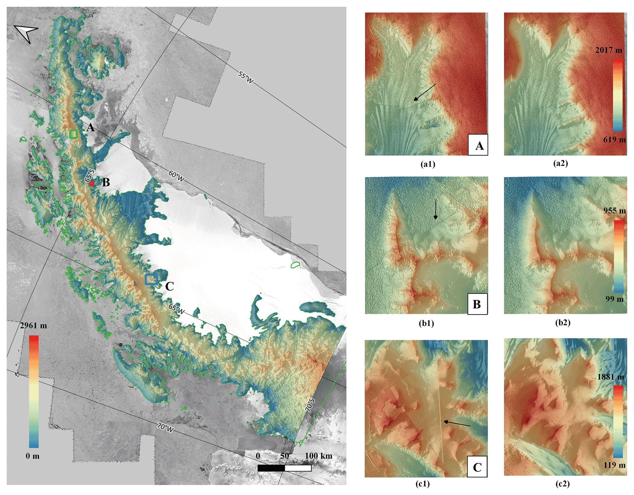
Figure 8 Left: corrected TDM DEM of the Antarctic Peninsula and the location of the sample areas. Right: comparison of the original TDM DEM (a1, b1, c1) with the corrected TDM DEM (a2, b2, c2) in the sample areas A, B and C. Black arrows point to the boundaries of the erroneous areas which have to be eliminated.

Table 3 Statistics of DEM elevation differences between the laser points and the REMA mosaic and the original and corrected TDM DEMs over the Antarctic Peninsula in Fig. 8. All elevation units are in meters. Elevation difference: DEM elevation minus laser elevation. We separately considered the statistics for points affected by elevation biases where correction was applied and those falling into unchanged areas.

5 Discussion

5.1 The effectiveness of the proposed method for the different elevation error patterns

The results presented in Sect. 4 demonstrate the effective elimination of the residual elevation errors in the TDM DEM product through validation with the high-precision laser altimetry data. Examples of residual elevation errors in the original TDM DEM product are visualized in the elevation difference maps (Figs. 6c and 7c), while the effects of the applied corrections are shown in Figs. 6f and 7f. In this section, the elevation errors and their removal in the TDM DEM are analyzed along several profiles located as in Figs. 9a and 10a and belonging to the experimental areas used in Sect. 4.1 and 4.2. From the profiles in Figs. 9 and 10b–e the erroneous elevations can be roughly divided into two patterns. Their influences on the effectiveness of the proposed method are evaluated qualitatively below.

In Fig. 9, the profile can be divided into sub-segments with similar offsets ranging from tens to hundreds of meters. Also, in Fig. 10d and e, spatially-connected points along the profiles L3 and L4 deviate from the correct elevation values with a certain offset. These jumps are much larger than the elevation difference between the TDM DEM and REMA mosaic and cannot be caused by the X-band microwave penetration depth (ranging from several meters to 10 m for high-penetration conditions) (Rizzoli et al., 2017b) or temporal surface elevation changes (−3 m/a at HG between 2013 and 2016) (Rott et al., 2018). Besides, the clear boundary in the DEM hillshade map (Fig. 9a) and the elevation jumps in the elevation profiles (Figs. 9 and 10b–e) further confirm the existence of the residual elevation errors and exclude the influence of signal penetration and temporal elevation surface changes. These kinds of local elevation offset are typical elevation errors introduced by PU due to the erroneous determination of phase ambiguity. The path propagation method described in Sect. 3.2 can automatically detect the local regions affected by elevation offsets and segment them into sub-regions with similar offsets. The correction method proposed in Sect. 3.3 takes the offsets between the TDM DEM and REMA mosaic in stable areas around the erroneous region into consideration, thus avoiding over-correcting the TDM DEM according to the REMA mosaic. As a result, the corrected elevation profiles are continuous and smooth (black lines in Figs. 9 and 10b–e) and the spatial details are well preserved even after eliminating the offset, e.g., as along profile L4 (Fig. 10e).

Unlike the local continuous region with similar elevation offsets, profile L1 (Fig. 10b) shows the elevation inconsistency pattern when the erroneous region neither has a unified elevation offset like L3 (Fig. 10d) and L4 (Fig. 10e) nor can be segmented into sub-regions with similar offsets and clear boundaries as in Fig. 9. The regional elevation offsets in Fig. 10b are still related to phase-unwrapping errors. However, the scene-based weighted average processing when generating the final TDM global DEM mosaic make it difficult to distinguish the original PU errors in the raw DEMs. In addition, the residual calibration errors may be introduced near a vertical offset and a horizontal tilt (and shift), thus contributing to the elevation inconsistency in the mosaicked TDM DEM. Under these circumstances, the elevation correction depends on the detected erroneous regions through the path propagation algorithm and is more influenced by the REMA DEM. Another particular case is shown for profile L2 (Fig. 10c) where elevation anomalies at a small horizontal spatial scale occur. L2 can be seen as a combination of different patterns where the proposed correction method can also work effectively by removing elevation offsets and noise.

Figure 9 Elevation profiles along the black line extracted from the (a) original and (b) corrected TDM DEM of the local sample area.

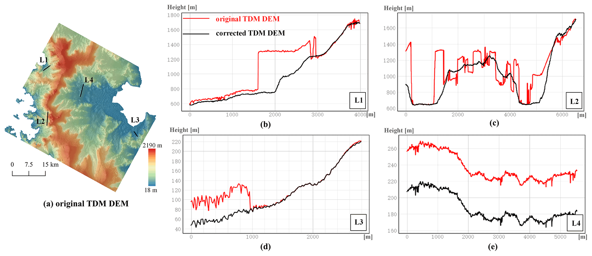
Figure 10 Four elevation profiles extracted along lines L1–L4 from the original and corrected TDM DEM in the HG area.

5.2 The importance of the multi-scale elevation error correction strategy

Taking into consideration the various vertical scales of the residual elevation errors, we proposed the multi-scale elevation error correction method in Sect. 3.4. Here we discuss the necessity of the multi-scale elevation error correction strategy as well as the validation methods.

In our experiments, we applied corrections of elevation errors at three scales: large (>45 m), medium (>20 m) and small (>5 m). These three thresholds were empirically determined from the intermediate correction results. In the following we explain in detail the process of multi-scale correction for the local and HG experimental areas. In the elevation difference maps of typical regions with PU errors such as in Figs. 11a and 12a, the elevation discrepancies have absolute values larger than 50 m. Then at the first correction, we set the threshold as 45 m to separate the background pixels. After this first iteration the remaining elevation discrepancies reduce to absolute errors larger than 20 m as visible in Figs. 11b and 12b. After applying the second correction (with a 20 m threshold), residual elevation offsets are still visible in the elevation difference maps (Figs. 11c and 12c). Therefore we set 5 m as the threshold for the small-scale correction. Besides using the thresholds for erroneous region detection, the correction also depends on the fitted reference elevation surface defined by the stable points extracted from the buffer zone. If there are not enough stable points, the correction will not be applied. To differentiate these small residual DEM elevation errors from elevation changes due to natural processes like the penetration depth or temporal surface change in the final small-scale correction, we also take the area of the merged regions into account. Considering the penetration depth and the temporal surface change affect a relatively large area and are changing with the transitional trend, only small regions (e.g., less than 100 pixels) with elevation jumps will be corrected during the third iteration. The magnitude of the elevation differences could be reduced gradually after each correction step as is obvious from the decreasing elevation range in the difference maps with the final improved results visible in Figs. 11d and 12d.

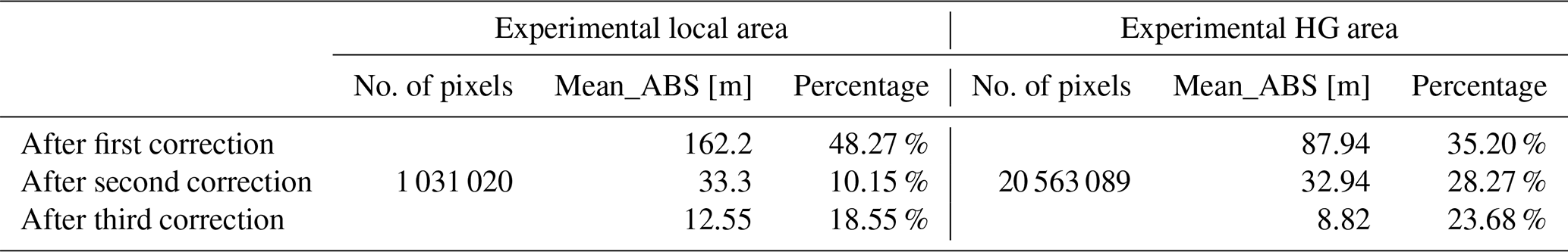
The corresponding elevation difference statistics after each correction when compared to LVIS 2015 and ATL06 2019 data are given in Tables S2 and S3 in the Supplement for the local and HG area, respectively. MAE and RMSE decrease significantly after each iteration. The mean of the absolute correction elevation (mean_ABS) and the coverage percentage for the detected elevation discrepancies (Table 4) diminish obviously after each iteration of correction.

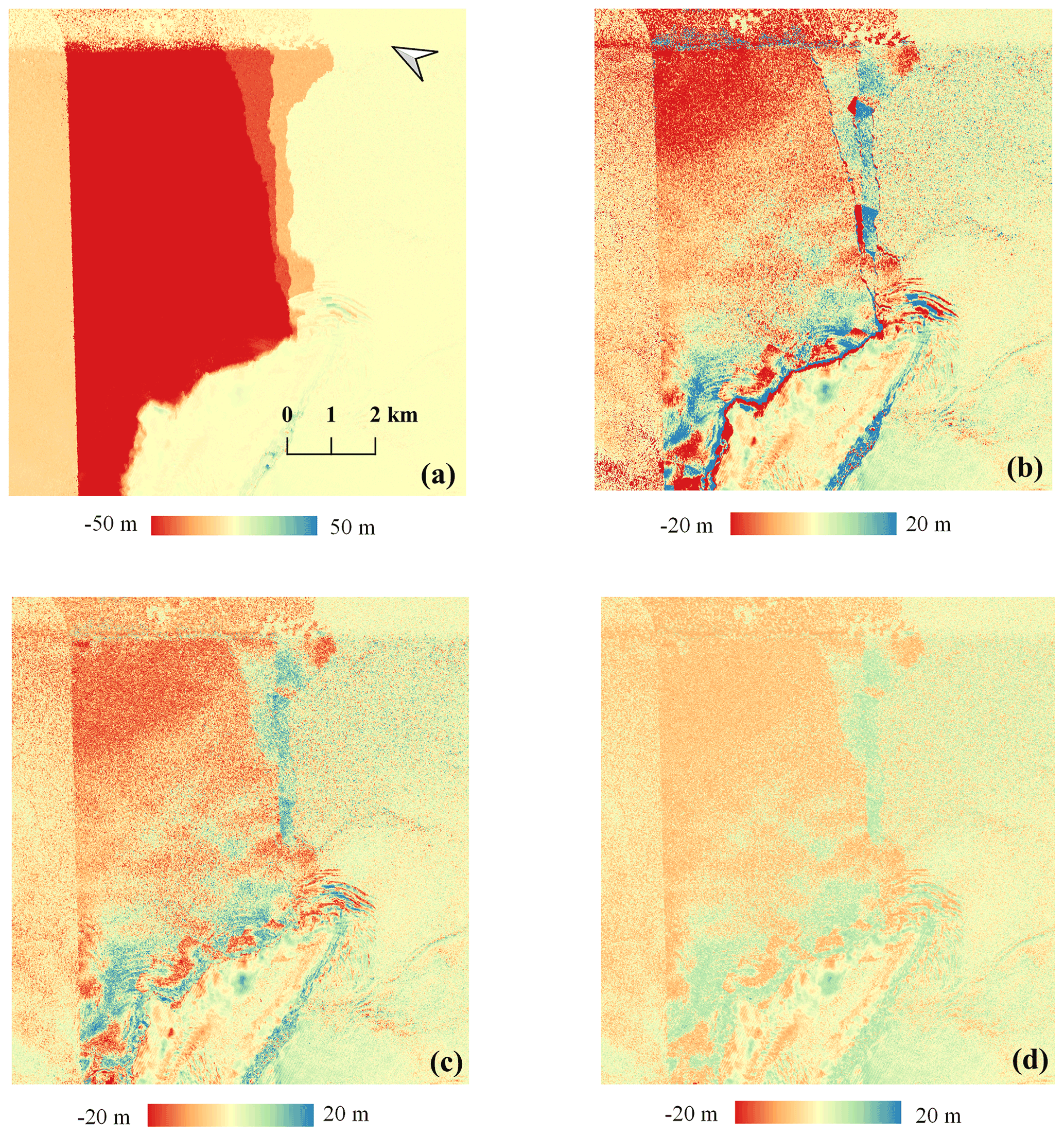
Figure 11 Elevation difference maps of the local area between the (a) original TDM DEM, (b) TDM DEM after the first multi-scale correction, (c) TDM DEM after the second multi-scale correction and (d) TDM DEM after the third multi-scale correction and the REMA mosaic. Elevation difference: TDM DEM minus REMA mosaic.

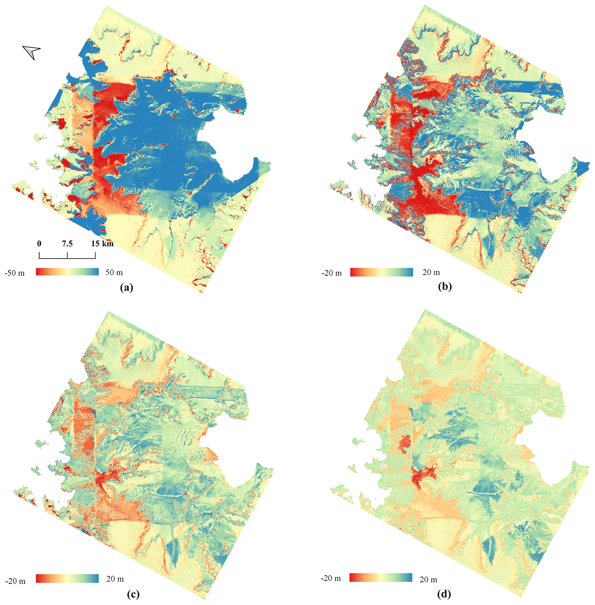
Figure 12 Elevation difference maps of the HG area between the (a) original TDM DEM, (b) TDM DEM after the first correction, (c) TDM DEM after the second correction and (d) TDM DEM after the third correction and the REMA mosaic. Elevation difference: TDM DEM minus REMA mosaic.

Table 4 The mean absolute correction value and coverage percentage for the detected elevation discrepancies.

5.3 The influence of reference DEMs' spatial resolution and data voids

The proposed method relies on absolute vertical accuracy and the spatial resolution of the reference DEM. The REMA mosaic has high absolute vertical accuracy and is generated from optical photogrammetry without PU errors (Howat et al., 2019), which is favorable for correcting elevation biases in the TDM DEM. Ideally the reference DEM should have a spatial resolution comparable with the DEM to be corrected like the 12 m TDM DEM and 8 m REMA mosaic. However, there are about 8 % gaps of the landmass in the 8 m REMA mosaic based on our statistics. In our experiments, the 8 m REMA mosaic has been resampled to the same spatial resolution as the TDM DEM of 12 m before the generation of the elevation map. The data voids of the 8 m REMA mosaic were filled by the 100 m REMA mosaic whose voids have been filled by the 100 m edited ASTER GDEM (Howat et al., 2019). Therefore, the analysis of the influence of data voids on the proposed correction algorithm is actually to analyze the influence of the different spatial resolutions between the original TDM DEM and the reference DEM.

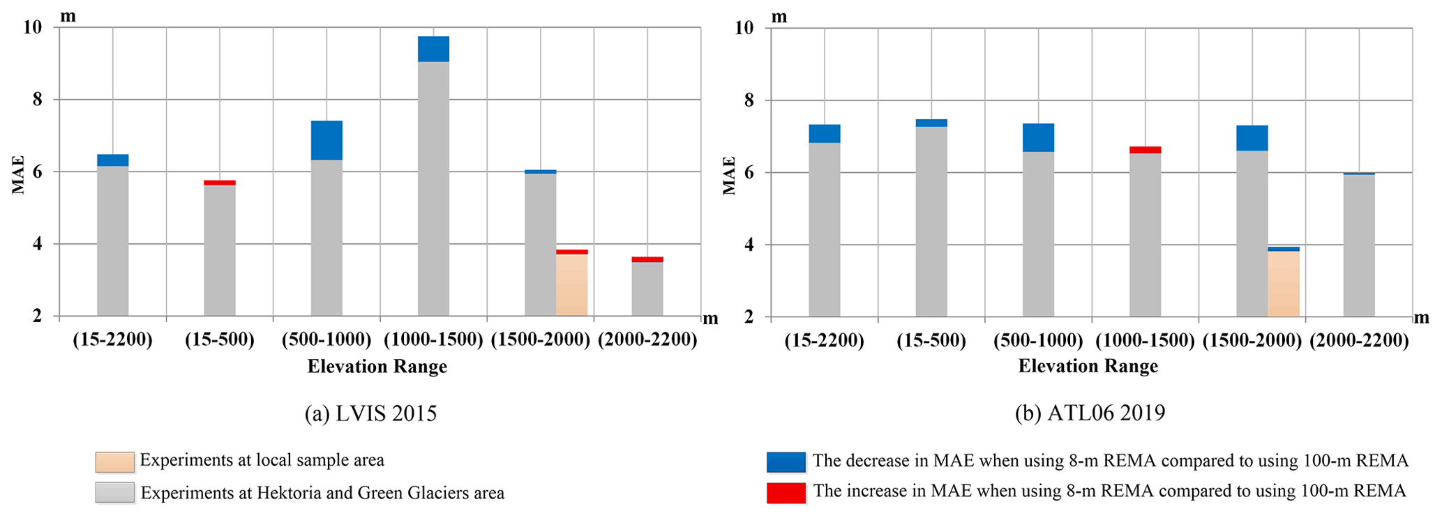
Figure 13 Changes in MAE of the corrected TDM DEM when using the 8 and 100 m REMA mosaic as ground reference. Results were evaluated against (a) LVIS 2015 and (b) ATL06 2019 datasets.

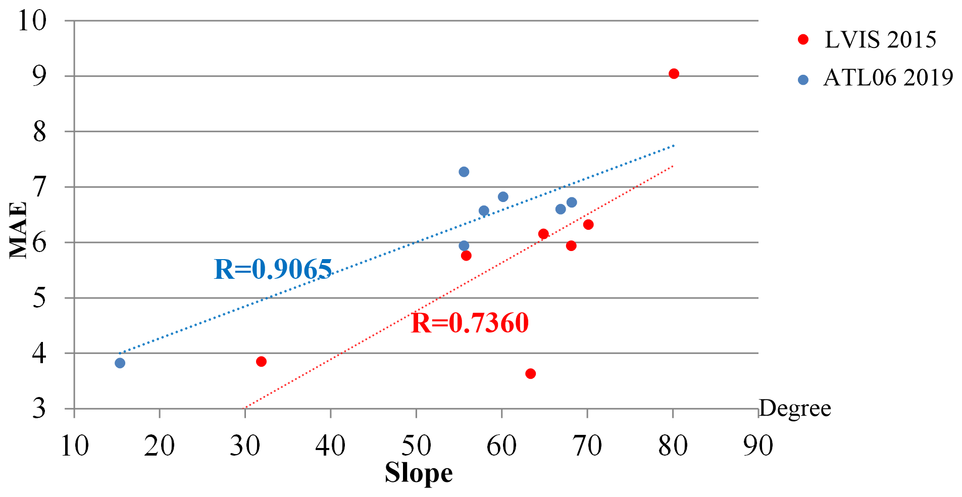
Figure 14 Linear regression between the MAE of the corrected TDM DEM using the 8 m REMA mosaic as ground reference and the median slope calculated from the corrected TDM DEM at the elevation ranges as in Fig. 13.

To evaluate the influence of the different spatial resolutions of the reference DEMs on the correction algorithm, we performed a contrast experiment here that uses the 8 and 100 m REMA mosaic as reference DEMs for correcting the original TDM DEM for two sample areas as in Figs. 11 and 12. The corrected DEMs were evaluated by the altimetry datasets LVIS 2015 and ATL06 2019 as in Fig. 13. In the HG area the MAE is overall higher for the corrected TDM DEM with the 100 m REMA mosaic compared to the 8 m REMA mosaic correction, while in the small local sample area the resulting MAEs are similar. The MAEs are affected by the location of the laser points. We calculated a linear regression of MAE and slope combining all the validation data of the two experimental sites (Fig. 14). The MAEs correspond to the corrected TDM DEM using the 8 m REMA mosaic as ground reference given in Tables 1 and 2. The median slopes were calculated from the corrected TDM DEM for the elevation range of each MAE value. A positive correlation between MAE and the terrain slope is observed, steep slopes being prone to large elevation errors in the DEM.

From the perspective of the algorithm implementation, the elevation biases can be detected and corrected by the proposed algorithm as long as they can be identified from the elevation difference map with distinguishable boundaries. Theoretically, the influence of the spatial resolution between different datasets depends on the spatial size of the regions with elevation biases and whether these regions have complex topography or not. Therefore the difference in the resolution of the reference DEM datasets has slighter impact on the correction algorithm on flat ground than in areas with severe terrain undulations.

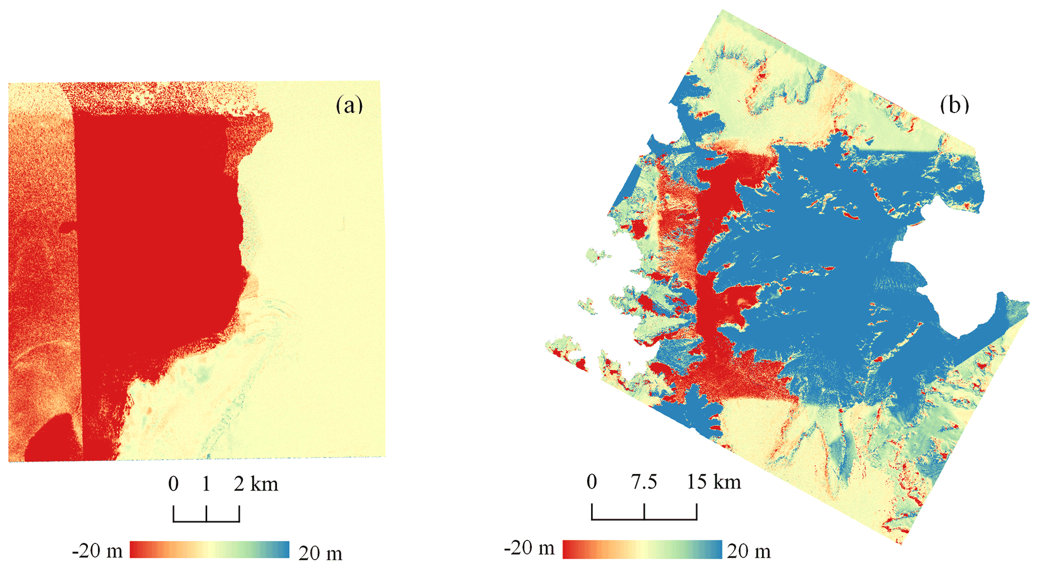
Figure 15 Elevation difference in the fused DEM minus the REMA mosaic in the (a) local sample and (b) HG area.

5.4 Potential applications of the corrected TDM DEM

The original TDM DEM and REMA mosaic have comparable absolute vertical accuracy according to our validation results in Table 3, but the TDM DEM has better completeness (Fig. S1), temporal consistency (Fig. S2) and relative vertical accuracy based on the elevation error layers accompanying the DEM products (Figs. S3 and S4). The residual systematic error correction of the TDM DEM is minimally influenced by temporal or penetration differences between the TDM DEM and REMA mosaic. The characteristics of an interferometric DEM are maintained, and therefore the outcome is not a hybrid DEM like it would be for a gap-filled REMA mosaic. This may bring advantages of using the corrected TDM DEM for certain applications. It can be used in specific interferometric processing like topographic-phase removal, PU corrections, geocoding, single-pass InSAR DEM generation and absolute-phase calibration. Having a precise time stamp and a short acquisition time span, the TDM DEM acquired in the austral winters of 2013 and 2014 can be subtracted from other DEMs to derive surface elevation change and geodetic mass balance of AP glaciers over a time span of several years. The TanDEM-X change DEM (Lachaise et al., 2019) generated from data acquired between 2017 and 2019 could be one of the candidates. With 12 m pixel spacing the corrected and gapless TDM DEM has certain advantages compared to the former gapless reference DEMs covering the AP like the 100 m edited ASTER GDEM (Cook et al., 2012), the 100 m REMA mosaic (Howat et al., 2019) and the 90 m TanDEM-X PolarDEM (Wessel et al., 2021) for glaciological applications and morphological analysis requiring a high spatial resolution. The corrected TDM DEM can also be used to fill the data voids in the 8 m REMA mosaic.

5.5 Comparison with DEM fusing method

To verify the effectiveness of the proposed algorithm in a comparative way, we fused the TDM DEM and REMA mosaic with weights determined by their random elevation errors as in Eq. (4). The difference maps between the fused DEMs and REMA mosaic over the experimental sites are shown in Fig. 15. Compared with the difference map before and after the correction in Figs. 11 and 12, it is obvious that the weighted fusion cannot eliminate the elevation discrepancies in the TDM DEM caused by PU errors because the HEM layer considered the random error used for weights determination is not capable of representing the PU errors. This contrast experiment well proves the effectiveness of the proposed algorithm in detecting and correcting the residual PU errors.

$$\begin{array}{}\text{(4)}& H_{\mathrm{fusion}}=\text{TDM}\mathit{\_}H\cdot \text{TDM\_weight}+\text{REMA}\mathit{\_}H\cdot \text{REMA\_weight},\end{array}$$

where $\text{TDM\_weight}=\frac{\mathrm{1}/\text{TDM\_error}}{\mathrm{1}/\text{TDM\_error}+\mathrm{1}/\text{REMA\_error}}$, $\text{REMA\_weight}=\mathrm{1}-\text{TDM\_weight}$, and TDM_H and REMA_H represent the elevation values from the TDM DEM and REMA mosaic.

6 Conclusions

In order to meet the high-resolution topography data demand of fine-scale glaciological research, we combined elevation information provided by two up-to-date large-scale high-resolution DEM products, the 12 m TanDEM-X DEM (TDM DEM) and the 8 m REMA mosaic product, to generate a high-resolution precise, consistent and gapless DEM of the Antarctic Peninsula (AP). Prior to the combination with REMA, the TDM DEM is characterized by good data consistency and few data voids but contains residual systematic elevation errors introduced by baseline calibration, geometric distortion and phase unwrapping (PU). The REMA mosaic has in turn high absolute vertical accuracy (about 1 m) and an absence of regional outliers. Combining the advantages of the TDM DEM and REMA mosaic, we identified the areas in the TDM DEM affected by errors with a path propagation algorithm and developed the multi-scale method to automatically correct the elevation errors in the TDM DEM. The effectiveness of the proposed method and the vertical accuracy of the resulting DEM were validated by visual inspection and laser altimetry data. The main findings of our research are as follows:

1. The path propagation algorithm can effectively detect erroneous regions with similar elevation offsets caused by remaining PU errors in the TDM DEM and separate them from unaffected areas. By merging the adjacent homogeneous pixels into one region and holding the further propagation at background and heterogeneous pixels, the procedure allows a successful identification of regions with different elevation offsets even with blurry boundaries.

2. The elevation offset compensation includes a fitted reference surface derived from selected stable points in the TDM DEM near the difference to the REMA mosaic and thus preserves the reference elevation surface of the TDM DEM. The elevation difference between the TDM DEM and REMA mosaic caused by the penetration depth of the X-band radiation and temporal surface change should be excluded from the elevation correction applied to the TDM DEM. Buffer zones created around each extracted erroneous region provide the abovementioned selected stable points, which in turn generate the compensation elevation value.

3. The multi-scale method can comprehensively correct the TDM DEM by iteratively adjusting from large- to small-elevation-scale errors. The corrected TDM DEM is superior in data consistency and completeness to the REMA mosaic.

In general, the DEM over the AP resulting from the combination of the TDM DEM and REMA mosaic maintains the characteristics of the interferometric DEM and has an improved quality due to the correction of the residual elevation errors. The absolute vertical accuracies of the corrected TDM DEM and the REMA mosaic validated against laser altimetry data (Operation IceBridge LVIS and ICESat-2) are very similar. We therefore recommend using the presented corrected DEM in various glaciological applications requiring detailed gapless topography information. The precise time stamp (austral winter 2013 and 2014) is an advantage for direct comparisons with other DEMs and derivation of surface elevation changes. Besides, DEM time series needed for the geodetic mass balance can be precisely vertically co-registered using our DEM as reference surface. In interferometric SAR processing the presented DEM can support the modeling of the topographic phase when separating this contribution from displacements and vertical deformation. Drainage basin delineations of individual glaciers also rely on accurate DEMs. The proposed method can be extended to other areas of the Antarctic Ice Sheet where SAR and optical DEMs are prone to errors, like mountainous coastal regions or in the Transantarctic Mountains.