the Creative Commons Attribution 4.0 License.
the Creative Commons Attribution 4.0 License.
 | 24 Aug 2021
An X-ray micro-tomographic study of the pore space, permeability and percolation threshold of young sea ice
Sönke Maus
Martin Schneebeli
Andreas Wiegmann
The hydraulic permeability of sea ice is an important property that influences the role of sea ice in the environment in many ways. As it is difficult to measure, so far not many observations exist, and the quality of deduced empirical relationships between porosity and permeability is unknown. The present work presents a study of the permeability of young sea ice based on the combination of brine extraction in a centrifuge, X-ray micro-tomographic imaging and direct numerical simulations. The approach is new for sea ice. It allows us to relate the permeability and percolation properties explicitly to characteristic properties of the sea ice pore space, in particular to pore size and connectivity metrics. For the young sea ice from the present field study we obtain a brine volume of 2 % to 3 % as a threshold for the vertical permeability (transition to impermeable sea ice). We are able to relate this transition to the necking of brine pores at a critical pore throat diameter of ≈0.07 mm, being consistent with some limited pore analysis from earlier studies. Our optimal estimate of critical brine porosity is half the value of 5 % proposed in earlier work and frequently adopted in sea ice model studies and applications. By placing our results in the broader context of earlier studies, we conclude that the present threshold is more significant in that our centrifuge experiments and high-resolution 3D image analysis enable us to more accurately identify the threshold below which fluid connectivity ceases by examining the brine inclusion microstructure on finer scales than were previously possible. We also find some evidence that the sea ice pore space should be described by directed rather than isotropic percolation. Our revised porosity threshold is valid for the permeability of young columnar sea ice dominated by primary pores. For older sea ice containing wider secondary brine channels, for granular sea ice and for the full-thickness bulk permeability, other thresholds may apply.
- Article
(4123 KB) - Full-text XML
- BibTeX
- EndNote


Sea ice is a porous medium that covers, on average, 5 % to 7 % of the earth's oceans. To understand the role of sea ice in the earth system, its hydraulic permeability needs to be known. A proper understanding of the salinity evolution of sea ice requires the knowledge of its permeability (Cox and Weeks, 1988; Worster and Wettlaufer, 1997; Petrich et al., 2006; Vancoppenolle et al., 2007; Wells et al., 2013; Griewank and Notz, 2013; Turner et al., 2013; Rees Jones and Grae Worster, 2014). Through its control of the salinity of sea ice, the permeability furthermore impacts the evolution of many other physical properties like sea ice strength and thermal conductivity (Cox and Weeks, 1988; Worster and Wettlaufer, 1997) that depend on the brine porosity of sea ice. Of high relevance for sea ice in the climate system is also the role of permeability for the melt pond albedo feedback: melt ponds from melted snow, appearing on sea ice during summer, will drain when the sea ice is permeable, exposing an ice surface that reflects more sunlight than ponded ice (e.g. Freitag and Eicken, 2003; Polashenski et al., 2017).
While permeability plays a key role for proper modelling and understanding of sea ice properties, observations are sparse and span, even at a fixed porosity, 2–3 orders of magnitude (Maksym and Jeffries, 2000). Test procedures used so far all suffer from shortcomings. Field measurements based on the filling rate of in situ boreholes only give some average measure of near-bottom permeability. These values further depend on the unknown permeability anisotropy and pore space details and thus are uncertain (Freitag, 1999; Freitag and Eicken, 2003; Golden et al., 2007). Laboratory studies have been restricted to relatively young and thin ice (Saito and Ono, 1978; Ono and Kasai, 1985; Saeki et al., 1986; Okada et al., 1999). To what degree these experiments resemble natural sea ice is uncertain and may only be answered by a comparison of microstructure and pore scales not performed so far. The most frequently cited study of sea ice permeability (Freitag, 1999) was based on samples from an ice tank experiment. Ice core segments were first centrifuged at in situ temperatures before the permeability was obtained experimentally with a kerosene-based permeameter set-up. The advantage of centrifuging ice samples and using a liquid that does not mix with water is to avoid microstructure changes that inevitably take place during storage and/or fluid flow. However, since the study by Freitag (1999) no further observations to validate the permeability values based on this method have been published. It is thus unclear to what degree the results are valid for natural sea ice and how different ice growth and age might affect the results.
The present study follows the centrifuging approach by Freitag (1999) and extends it in several ways. First, the permeability of centrifuged sea ice samples is not determined by a laboratory permeameter but through direct numerical simulations on 3D X-ray micro-tomographic (XRT) images. Second, we perform a statistical analysis of the 3D XRT-based pore space that allows for a physical interpretation of permeability in terms of pore sizes and connectivity. Third, we extend the porosity range documented so far to values when the ice becomes impermeable, obtain an estimate of the threshold porosity and analyse the pore space near the threshold. Our approach allows us to revise the percolation threshold of ϕ≈0.05 that has been proposed in earlier studies without consideration of the microstructural pore size details (Petrich et al., 2006; Golden et al., 2007). Furthermore, we present a relationship between permeability and brine porosity that is valid over a wider range of porosities than so far investigated.
2.1 Field sampling
Sea ice samples for the present study were obtained from fast ice in Advent Bay of Adventfjorden, Svalbard, during 14 to 19 April 2011, approximately 2 km from the UNIS (University Courses on Svalbard) building (Fig. 1). The meteorological conditions indicate, in combination with daily ice charts from the Ice Service of the Norwegian Meteorological Institute (https://cryo.met.no/archive/ice-service/icecharts/quicklooks/, last access: 11 August 2021), that the ice was approximately 3–4 weeks old. After most likely freeze-up during 20–22 April 2011, it mostly grew during a period of 10 d with temperatures around −20 ∘C, followed by 10 d with gradual warming. A 10 cm cover of new snow on the ice had mostly accumulated a few days prior to sampling. The insulation through the snow cover resulted, in spite of air temperatures varying by 7 K during the sampling period, in only minor ice temperature changes over 5 d and a temperature range of less than 1 K over 35 cm thickness. While originally sampling of ice at different temperatures was planned, the stable temperature turned out to be an advantage for temperature control and allowed us to harvest and analyse ice cores of very similar salinity and structure and rather to perform a controlled cooling sequence in the laboratory.
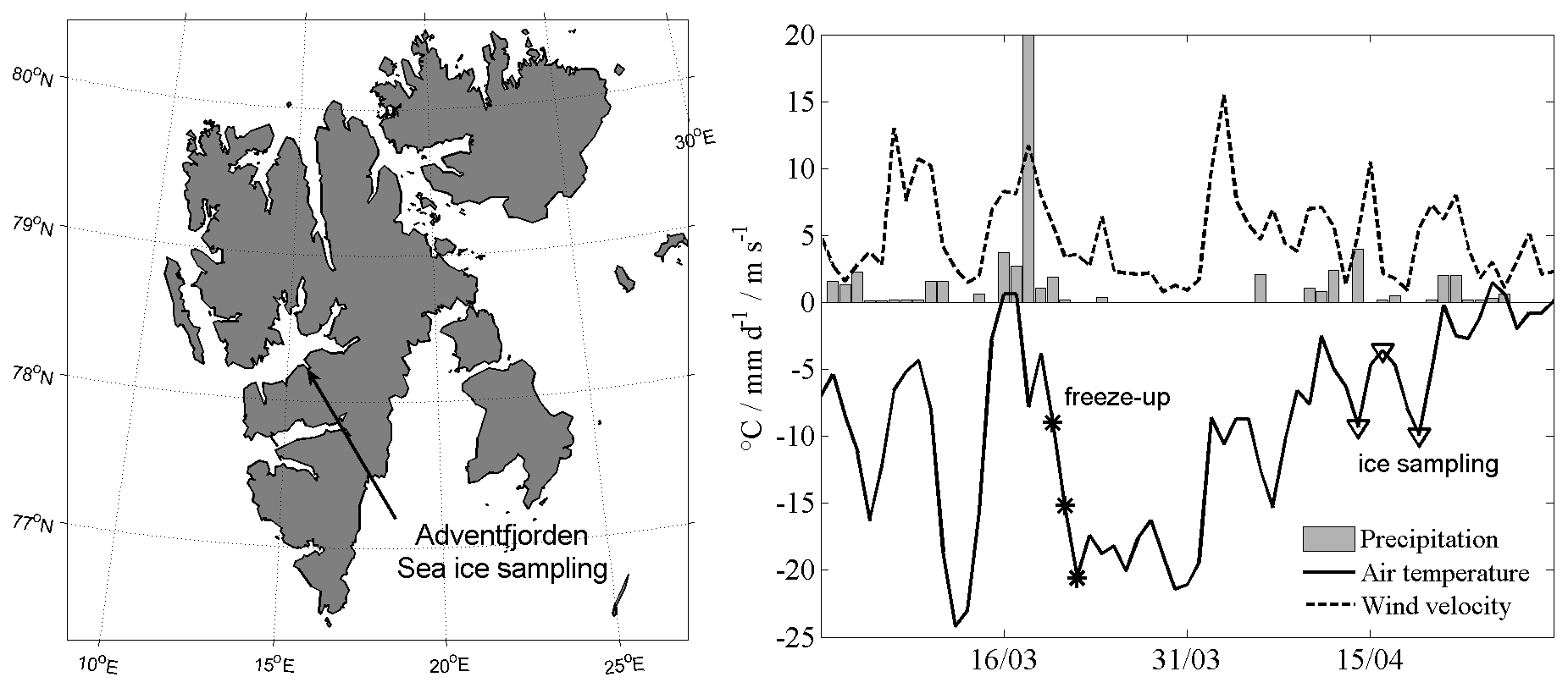
Figure 1Left: location of sampling of young sea ice in Advent Bay of Adventfjorden. Right: meteorological conditions at Longyearbyen airport in March/April 2011, from freeze-up (*) to sampling 3 to 4 weeks later (▿).
During each sampling date six full ice cores were obtained with a 7.25 cm diameter coring device (Mark III, Kovacs Enterprise) from 35 cm thick fast ice. Cores were immediately cut into 3–4 cm thick sub-samples. On a first ice core, temperatures were measured with a penetration probe; this core was only used further for temperature tests. All other core segments were packed in plastic beakers, stored in an isolating box and rapidly (by snow mobiles, within 30 min from the beginning of coring) transported to the UNIS laboratory. For the given field conditions the temperature change that samples may have experienced during this transport might be a few tenths of a Kelvin (see below in Sect. 2.5). We note that less isothermal ice would have required a more advanced temperature control of the different levels in the ice. At UNIS the samples were moved into temperature-controlled freezers (WAECO CoolFreeze T56) close to their in situ temperatures (typically within 0.3 K). During the three sampling dates a total of 15 ice cores were obtained and sectioned into 145 sub-samples.
2.2 Laboratory cooling sequence
In situ sea ice temperatures were in the range of −2 to −3 ∘C. To extend this natural range we used the following approach in the laboratory. For each of the three sampling dates one core was left at in situ temperatures. The sub-samples from the four replicate cores were put into freezers controlled at lower temperatures of −3, −4, −6, −8 and −10 ∘C and equilibrated by 1 to 3 d. The result is, for each level in the ice, a series of five samples with temperatures gradually ranging between in situ values (−2 to −3 ∘C) and minimum temperatures in the range of −8 to −10 ∘C. In this way we generate samples with up to 4.5 times smaller brine porosity compared to the in situ condition.
2.3 Centrifugation
In a laboratory at UNIS the sub-samples were centrifuged in a refrigerated centrifuge (Sigma 6K15). In our protocol the sub-samples were placed on the field site into conical buckets to collect the brine that drained from them during storage. Centrifuging was performed 1 to 4 d after sampling, with longer waiting time for those samples cooled to lower temperatures. To do so, samples were placed into flexible stainless steel tea sieves that fitted into the conical plastic buckets. Centrifuging thus extracted the brine from brine channels with a downward orientation, open to the bottom or perimeter of the sub-sample.
Centrifuging was performed at in situ temperatures (one core) and at the lowered temperatures from the sequence (four cores). The centrifuged ice samples were immediately after centrifugation set into a −80 ∘C freezer. Next the mass of centrifuged brine and residual ice samples was measured. The centrifuged samples were then cut down from the initial 7.25 to 3.5 cm diameter, and the ice that was cut off was melted. The centrifuged brine and melted residual ice were filtered with a 100 µm sieve before the salinity was determined via measurements of the electrolytic conductivity and temperature (WTW Cond 340i instrument). Brine samples with salinity >40 g/kg were diluted to perform the conductivity–salinity conversion with seawater standard formulas. Salinity values obtained in this way have a measurement accuracy of better than 0.2 g/kg.
A duration of 15 min and a centrifuge acceleration of 40 g (earth gravity) were selected for centrifuging. These numbers have been chosen due to several aspects of the approach. The acceleration ensures a pressure force (40ρigH) of less than 15 kPa, well below the lowest tensile strength values (20–50 kPa) observed for natural sea ice (Weeks, 2010). This ensures that samples do not deform internally during centrifuging, though it could not prevent the compression and micro-fracture of the fragile ice–seawater interface sub-sample. Second, it is important to set the centrifuge temperature close to but slightly (0.5–1 K) below the sample temperature because otherwise the samples may warm up in the end and release additional brine. A third aspect, the impact of parameter choice on proper brine removal, is discussed below in connection with the permeability simulations.
As discussed in earlier applications (Weissenberger et al., 1992; Freitag, 1999; Krembs et al., 2001), centrifuging gives important information about the disconnected and connected fractions of the brine pore space. The centrifuged porosity may be associated with the effective porosity ϕeff relevant for fluid flow and permeability (Freitag, 1999), for which we shall use ϕcen henceforth. Let the total brine porosity ϕ be the sum of the centrifuged brine porosity ϕcen and the residual brine porosity ϕres. Assuming that the corresponding brine salinities are the same, these porosities may be determined from salinity determinations alone:
where Si is the bulk salinity of the original ice sample, Sir the residual salinity of a sample after centrifugation and Sb the salinity of the centrifuged brine; ϕ was determined from Si and temperature Ti, assuming thermodynamic equilibrium and applying equations from Cox and Weeks (1983).1 The centrifuged and cut ice samples were further stored in a −80 ∘C low-temperature freezer and kept for 2 months at this temperature (including transport on dry ice). The samples were equilibrated to −20 ∘C 2 d prior to imaging by X-ray micro-computed tomography (XRT) described below.
The centrifuge parameters depend on centrifuge type and were carefully chosen on the basis of several tests. (i) Ice samples were centrifuged with temperature loggers to determine temperature stability. Slight warming of the centrifuge was observed, leading us to the choice of an initial centrifuge temperature 1 K below the ice in situ temperature. A similar value was chosen by Weissenberger et al. (1992) for similar centrifuge times. (ii) Varying the centrifuging time from 10 to 20 min showed that more than 95 % of brine was extracted during the first 10 min, and we selected 15 min. (iii) Freitag (1999) noted that incomplete centrifugation of brine might lead to brine remnants which, after cooling and freezing, might block pores and decrease the permeability. We have indeed found such a result in an earlier study with centrifuge acceleration of 15 g (Buettner, 2011) and thus tested the effect of relative centrifuge acceleration for three ice cores at 10, 25 and 40 g. The result was on average 20 % less centrifuged brine at 10 g but only a slight non-significant 5 % difference between 25 and 40 g. We thus are confident that 40 g is a proper choice for extracting the connected brine.
The centrifuged brine mass on which the effective porosity is based also includes brine that has leaked from the sample during storage, prior to centrifuging. In our study this pre-drained brine volume was not negligible and contributed on average 28 % of the total (leaked and centrifuged) brine volume. On the one hand this value may be an overestimate as it could include small ice particles that fell into the cup during sampling. On the other hand, there is very likely some brine lost during coring and cutting, which will underestimate the centrifuge-based effective porosity. Both effects imply a difference between CT-based and centrifuge-based estimates of effective porosity that we cannot resolve with our data.
2.4 X-ray micro-tomography
X-ray tomographic imaging was performed at the WSL Swiss Federal Institute for Snow and Avalanche Research, Davos, Switzerland, with two desktop cone-beam microCT instruments (MicroCT 40 and MicroCT 80, Scanco Medical AG) that operate with a microfocus X-ray source (7 µm diameter) and detectors of 2048×256 and 2048×128 elements, respectively. The instrument was located in a cold room at −20 ∘C. However, the temperature within the CT chamber was slightly higher, −16 ∘C. The samples, after centrifugation reduced to 35 mm diameter, were again slightly reduced to fit into the 35 mm diameter sample holders and then scanned with a 37 mm field of view, yielding a nominal pixel size of µm. Scanning time was roughly 1 h per centimetre sample height and thus 3–4 h per sub-sample. A total of 1000 images per 360∘ rotation were obtained. For the image analysis, 1200×1200 pixels were horizontally cropped from the centre of the 2048×2048 field of view and 1500 pixels vertically. The resulting XRT grayscale images were stored as 16 bit stacks and filtered with ImageJ (rsb.info.nih.gov/ij/), applying a 2 pixel median and Gaussian blur filter (standard deviation 1.5).
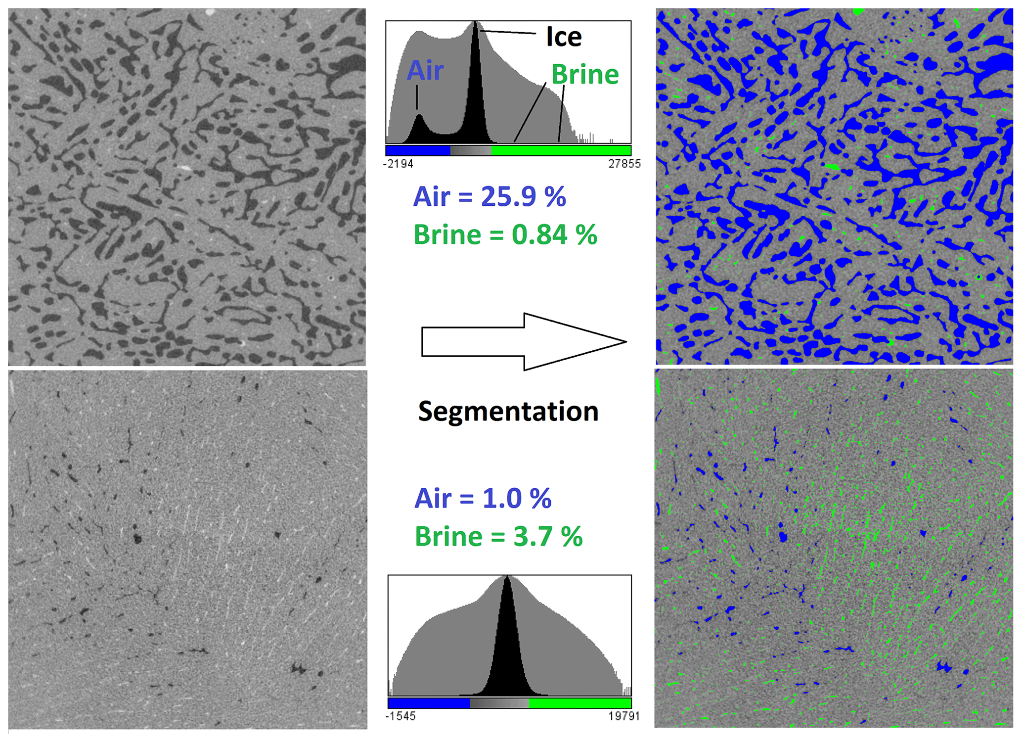
Figure 2Segmentation of pre-filtered greyscale absorption images (left) into the classes of air (blue), brine (green) and ice (grey) for a high-porosity (upper) and low-porosity (lower) image. The images in the middle give the histograms of grey values with a linear (black) and a log (grey) scale. Upper example: a high-porosity image with a well-defined air peak, yet little entrapped brine. Lower example: a sample with more entrapped brine than air or centrifuged brine.
The image segmentation into air, ice and brine was also performed with ImageJ as illustrated in Fig. 2 for two samples, one with high air and low residual brine porosity and another one with low air and moderate brine porosity. Our approach to find the air–ice and ice–brine thresholds was as follows. First, brine was ignored, and a global threshold that separates air and ice was found on sub-images with approximately equal fractions of air pores and ice, using Otsu's method (Otsu, 1979). Comparison with manual segmentation of single thresholds indicates an accuracy of 0.5 % to 1 % for the air porosity, being higher at high porosities. For the ice–brine threshold it was more difficult to find an automated procedure. Segmentation with Otsu's algorithm gave generally too high brine content (compared to direct measurements). The best results, comparing to measured salinity, were obtained within ImageJ using the so-called triangle algorithm, yet still with considerable scatter. It was thus decided to rather use an empirical approach that sets the ice–brine threshold to 1.20 times the grey value of the ice mode. This number led to the least deviation of average CT-derived salinity and the salinity of melted samples. However, also here the absolute uncertainty in brine volume was 0.5 % to 1 %, corresponding to a relative uncertainty of 30 %–100 % as residual brine porosities at −16 ∘C were low. Hence, the relative accuracy in residual brine determination is much smaller than for the air porosity. As the most likely explanation, it is considered that brine inclusions were not much larger than the voxel size and that brine is often found together with tiny air bubbles. This implies a considerable number of mixed air-brine pixels that have a grey value just a bit larger than ice.
Hence, for the present pore sizes, spatial resolution and brine salinity (≈185 g/kg at −16 ∘C), there are considerable uncertainties in ice–brine segmentation, and an unsupervised approach (i.e. without setting a threshold based on alternative bulk salinity measurements) was not found. However, the permeability is little or not affected by the residual brine and rather relates to the open air porosity (centrifuged, connected brine) that was determined with reasonable accuracy.
The imaged samples, cylinders with 35 mm diameter and 25–30 mm height, were again subdivided vertically into samples of 5.5 mm height. The subdivision is important for proper determination of permeability and percolation as for 20 mm high samples a considerable fraction (10 %–30 %) of slightly (10 to 30∘) inclined pores are running off at the vertical sides. Examples of these 3D sub-images to be analysed here are shown in the sections below. With the current imaging settings and image processing for analysis and simulations, we expect to observe pores and inclusions with the smallest dimensions of 36 µm (corresponding to a Nyquist criterion of 2 times the voxel size of 18 µm). This is an improvement by a factor of 2 compared to the voxel size of 41.5 µm in the CT image study of laboratory-grown ice by Pringle et al. (2009). Our horizontal scale is large enough to also observe pores and brine channels situated between grains of typical dimensions of 5 to 20 mm. Our standard vertical scale of 5.5 mm is smaller than used in standard sea ice bulk sample analysis of several centimetres, yet we can always merge the sub-samples to look at comparable vertical scales. The chosen horizontal and vertical sample scales are well above the typical pore scale characteristics of young ice obtained by Eicken et al. (2000) based on the analysis of magnetic resonance images with lower resolution (0.09 mm voxel size).
2.5 Sampling, transport, storage and textural changes
Special care was taken to minimize undesired temperature changes and variability prior to centrifugation and imaging. The cut samples of the relatively isothermal sea ice were transported in an Isopore box (inside a larger insulated aluminium box) to the laboratory. Transport and sorting into small temperature-controlled freezers happened within half an hour. As each sub-sample was packed in a conical plastic cup, temperature changes are, due to the large effective specific heat capacity, considered negligible. The box temperature was logged by a temperature logger, and temperatures were directly measured on samples, being within 0.2 K of in situ values. The next step, cooling of sub-samples in the laboratory, took place within these freezers set to lower-than-in-situ temperatures. With samples within the plastic cups, cooling rates (with most heat loss due to internal freezing) were moderate and in the range 1–5 K per day, comparable to natural cooling rates. An important aspect of the approach was also that samples were only cooled, not warmed. This avoids the known hysteresis that brine expelled during cooling is not reintroduced into a sample upon warming.
Though we have no strict proof for this, we believe that microstructure changes during 1 to 2 d of close-to-isothermal storage are minor (this is based on unpublished work of repeated scanning). More relevant could be effects due to freezing and redistribution of brine. First, one could expect that simultaneous cooling of sub-samples from all sides may redistribute brine in a way that differs from mostly vertical heat loss of ice in the field. We do not find brine accumulation in the centre of samples, indicating that also the multi-directional sample cooling redistributes brine along the predominantly vertically oriented pores. Brine could be redistributed vertically in some non-uniform way within a 3 cm thick sub-sample, and implications are considered in the discussion. Second, we treat our sample isothermally, which is justified as the in situ temperature profile suggests a difference of 0.1 K along the vertical direction. Third, sample storage after centrifugation at a low temperature (−80 ∘C) has likely led to almost complete precipitation of all residual brine. During XRT imaging these salt crystals have dissolved again. As the microstructure of these pores will very likely differ from field values, we do not analyse it here. We regard it as unlikely that this hysteresis of disconnected pores has affected the networks of connected pores.
We finally note that the small in situ temperature range made this study logistically easier as if the ice had been sampled during a cold period.
2.6 Permeability simulations
Flow through porous media at relatively low velocities is governed by Darcy's equation (Dullien, 1991; Nield and Bejan, 1999). In one dimension,
gives the dependence of average velocity (discharge per unit area) on pressure gradient d, dynamic viscosity μ of the fluid and permeability K. The latter has dimensions of area and may be imagined as the cross-section of an equivalent channel of fluid flow through the pore space. The present approach to obtain K is to centrifuge the brine from the pore space, store the samples, and later perform permeability experiments (Freitag, 1999) or computational fluid dynamics (CFD) simulations (Maus et al., 2013). It is thus of interest how the settings during centrifuging may impact the results: consider the pressure gradient across a sample filled with brine of density ρb. Inserting this into Eq. (2) one obtains the relationship
where the kinematic viscosity ν has replaced . This equation actually states the conversion from hydraulic permeability K to hydraulic conductivity . Replacing this bulk flow by ϕeffV, where V is the actual velocity within pores contributing to the flow, the condition for brine removal from a sample of height H during time t requires . Further replacing g by the effective geff in the centrifuge, we can write Eq. (3) as
as a condition for full removal of brine during centrifuging. With at the lower end of our porosity range (see below), sample thickness H=0.04 m, centrifugal time t=9000 s, m2 s−1 (at −10 ∘C) inserted into Eq. (3), and geff=40 g, we obtain m2. In ice samples with a lower permeability than that value, one can expect incomplete removal of brine. Upon cooling this brine will partially freeze and may render the sample impermeable. As we find below, the lowest simulated permeability value in our study is m2, close to the latter estimate. However, below we also find that ϕeff is much lower than ϕ when low porosities are approached, decreasing this limit for K by at least a factor of 3–4. We thus assume that insufficient brine removal during centrifuge acceleration is not a large problem for our results.
Here we report on vertical permeability computations that have been performed with GeoDict “Geometric Material Models and Computational PreDictions of Material Properties” (GeoDict, 2012–2021). The simulations were run on the mentioned sub-images of voxels (300 corresponds to 5.5 mm height) with the SimpleFFT solver of the FlowDict module in GeoDict. The solver obtains, for a given pressure drop across the sample, the stationary fluid flow on a uniform grid based on the iterative solution of the Stokes–Brinkman equation (Wiegmann, 2007; Cheng et al., 2013; Linden et al., 2018). Recent work has demonstrated the quality of the numerical solution of the FlowDict solver in comparison to observations (Zermatten et al., 2011; Gervais et al., 2015; Gelb et al., 2019). In our set-up a 10 voxel thick inflow region at the top and bottom of the sample was used in connection with periodic boundary conditions. Computations on 3D images with dimensions of ( mm) typically required 25–30 GB of RAM. Limiting the accuracy to 1 % appeared to be sufficient for most samples to converge in between 200 and 600 iterations, which typically took 1 to 3 d per sample on a four-core PC with a 3 GHz CPU. Simulations performed for 150 images have been published (Maus et al., 2013). The latter results have been revised in the present study, and simulations have been repeated for those samples that had not reached the convergence criterion (mostly low porosity and permeability samples). With currently faster hardware and improvement of the GeoDict solver, simulations are nowadays 10 to 20 times faster.
2.7 Pore space analysis
The permeability K of a porous medium (Eq. 2) is often parametrized in terms of total porosity in the form K∼ϕb, where the range has been found in observations (Dullien, 1991; Happel and Brenner, 1986). A more concise and physically consistent formula for the permeability is (e.g. Paterson, 1983)
wherein ϕeff is the effective porosity for fluid flow, Dc a characteristic pore diameter, τ tortuosity of the flow path and a a constant. For simple flow geometries this relationship is exactly known; e.g. for a bundle of parallel cylindrical pores of diameter Dc with cross-sectional area ϕ=ϕeff, one has τ=1 and , while for a system of parallel vertical lamellae (flow through slits of width D) with ϕ=ϕeff, one has (e.g. Paterson, 1983; Dullien, 1991). In more complex networks with a distribution of pore sizes, one has to find a characteristic pore scale Dc; tortuosity τ and a will depend on the detailed network morphology. Here we shall investigate how Dc, τ and ϕeff all depend on total porosity to understand for which regime a simplified relationship K∼ϕb is valid.
2.7.1 Porosity and volume fractions
In the present study we shall neglect solid salts. Including solid salts in the calculations would decrease brine volume fractions at the lower end of our porosity range by 0.1 %–0.2 % (see Cox and Weeks, 1983) and have little effect on our results. We divide the total porosity of sea ice into the volume fractions of brine ϕ and air ϕa. The porosity metrics relevant for our study are summarized in Table 1. In general, the brine porosity ϕ is considered to be the sum of a connected (infinite cluster) part ϕeff and a closed (disconnected) part ϕ−ϕeff. We use both ϕcen from centrifugation and ϕopn from the CT image analysis to estimate the open porosity. The closed brine porosity can be obtained either from the salinity of melted centrifuged samples ϕres or by image analysis ϕcls. Air porosity ϕa is only available through CT image analysis.
The open and closed fractions may be scale-dependent; e.g. a closed cluster of brine inclusions could appear open in small samples. Another effect of finite sample sizes is that, because channels are not strictly vertical, some are running out to the sides. The porosity metric relevant for the permeability simulations is thus the volume fraction that connects the upper and lower side of an ice sample, henceforth noted as connected porosity ϕzz.
For the air porosity we assume that all air is contained in closed-air inclusions entrapped in the ice and just define one ϕa term. Air bubbles contained in open brine pores are not detected by our approach as they likely are centrifuged out with the brine.
We obtain the porosity metrics ϕopn, ϕa, ϕzz and ϕcls with the GeoDict module PoroDict, which can be set to determine for any material the porosity open to a specific side (we use all sides) of a CT image. While ϕopn and ϕzz are associated with the centrifugation temperature (−2 to −10 ∘C), the porosity fraction ϕcls has to be obtained from the brine porosity ϕcls16 imaged at the CT operation temperature (−16 ∘C) by using the equations from Cox and Weeks (1983).

2.7.2 Pore size characteristics
We define characteristic pore scales in correspondence with the different porosity metrics given in Table 2. For the pore space analysis we also used the GeoDict module PoroDict. It offers two algorithms to obtain a pore size distribution (GeoDict, 2012–2021).
The first uses a sphere fitting algorithm to determine the fraction of the pore space that belongs to a certain diameter interval. The algorithm thus determines the minor axis of a cylinder with an elliptical cross-section. This is done for open- and closed-air-pore and open- and closed-brine-pore classes. From the distribution we obtain the median, in terms of volume. The results from this analysis are the open-brine-pore size Dopn, the closed-brine-pore size Dcls and the air pore size Dair.
Table 2Characteristic pore scales.
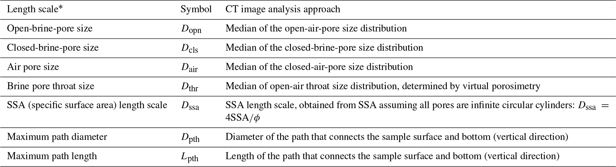
All median values are volume-based.
The second algorithm is based on the virtual injection of spheres into the sample to determine the fraction of the pore space that can be accessed through a sphere of a given radius. The latter is a porosimetry (e.g. Dullien, 1991) algorithm that determines an effective volume distribution of pores limited by throats and is termed throat size in the following. We obtain the median throat size Dthr as a global measure by injection of spheres from all six directions.
We obtain two further characteristic length scales. One is the maximum path diameter Dpth, which is the maximum diameter of a sphere that can pass through the sample. This length scale is of interest for the permeability, and it is easy to determine. The second length scale is based on the specific surface area (SSA) of the samples (here defined as internal surface per sample volume), also determined in PoroDict. If all pores are uniform and parallel cylinders, then their diameter may be related to SSA through , which shall be defined here as length scale Dssa.
3.1 Temperature and salinity
The ice thickness (35 cm on average) did not change measurably during our sampling period; the thickness range was 33 to 36 cm for the 18 cores obtained. Here we focus mostly on the cores obtained on 16 April 2011, and all cores from this date were CT-scanned and analysed using the methods described above. The ice had a surface (ice–snow interface) temperature of −2.9 ∘C and a near-bottom interface near the freezing point of seawater (−1.9 ∘C). Note that due to a 10 cm snow cover, the ice temperature from the other two sampling dates, 2 d earlier and later, was very similar. Figure 3a shows the in situ temperature profile as well as the temperatures to which the five microstructure cores were lowered prior to centrifugation. Figure 3b and c show the corresponding salinity profiles and brine volume profiles. For the brine volume the in situ values are also given as black dots.
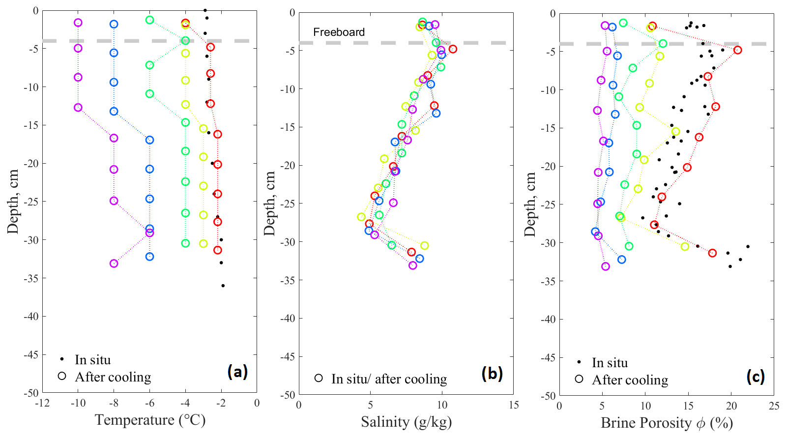
Figure 3Properties of 5+1 sea ice cores obtained on 16 March 2011 in Advent Bay, Svalbard. (a) In situ ice temperature shown as black dots, five lowered centrifugation temperatures as coloured circles. (b) Bulk salinity obtained from centrifuged brine and melted residual ice in colours. (c) Brine porosity ϕ based on thermodynamic equilibrium shown. Black dots show in situ values, while coloured circles give the brine porosity for the lowered centrifugation temperatures.
The salinity of the ice was obtained from mass and salt balance of the centrifuged brine and the cut residual ice samples. We also obtained salinity profiles for the earlier (14 March 2011) and later (19 March 2011) sampling dates (and did the same cooling and centrifuging experiments). As for the ice thickness, the salinity did not change measurably during this period. The salinity profile shows the well-known C shape, with some indication of drainage at the very surface above the freeboard.2 All five salinity profiles are very similar and show little variability. This gives confidence that the temperature dependence during our cooling sequence, not internal variability in the cores, will dominate the results.
3.2 Porosity
3.2.1 Centrifuged porosity
In Fig. 4a the centrifuged brine porosity ϕcen obtained in the centrifuge experiment is shown in dependence on the total brine porosity ϕ. This plot is based on all 15 ice cores from the three sampling dates, and thus 145 sub-samples of 3–4 cm thickness. The data indicate that at a certain total porosity ϕc the ϕcen becomes zero. To find this threshold we have regressed ϕcen against (ϕ−ϕc)β to obtain the optimum pair of ϕc and the critical exponent β. The result is the equation
and is shown in Fig. 4a as a dashed red curve. Figure 4b shows the regression results in terms of the dependence of β on ϕc. The red curve shows the maximum R2 corresponding to this β(ϕc) curve. The maximum R2=0.96 is found at ϕc=0.0240. For the exponent β=0.832 the 95 % confidence bounds from the log fit are [0.803, 0.861]. For the critical ϕc we obtain confidence bounds by using and ϕc=0.0240 as input to a power law regression, which in turn resulted in a 95 % bound range of . Note that a linear fit with β=1 would give ϕc=0.011, as we calculated earlier (Maus et al., 2013). The present analysis shows that the critical exponent β differs significantly from one.
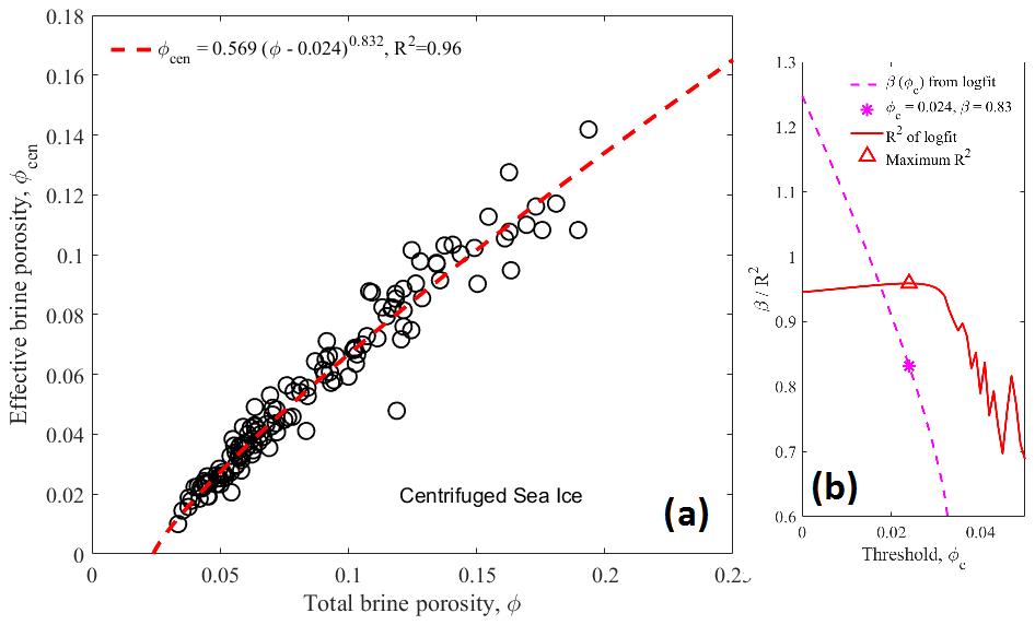
Figure 4(a) Relationship between centrifuged brine porosity ϕcen and total brine porosity ϕ based on 3–4 cm thick samples from 15 young ice cores of 35 cm length. (b) Optimum exponent β in dependence on porosity threshold ϕc and the R2 of double-logarithmic least-squares fits of ϕcen versus (ϕ−ϕc)β. The point of maximum correlation is shown as a star.
3.2.2 CT-based open porosity
The CT imagery allows us to view the morphology of closed and open pores in some detail, which is illustrated in Fig. 5a to c. For better visibility Fig. 5a is cropped from the centre of the original image (to horizontally). Ice is made invisible to illustrate the disconnected (in green) and connected pores (in red). Connected is used here synonymously with open, that is the pore is open to any of the six lateral boundaries of the 3D image.
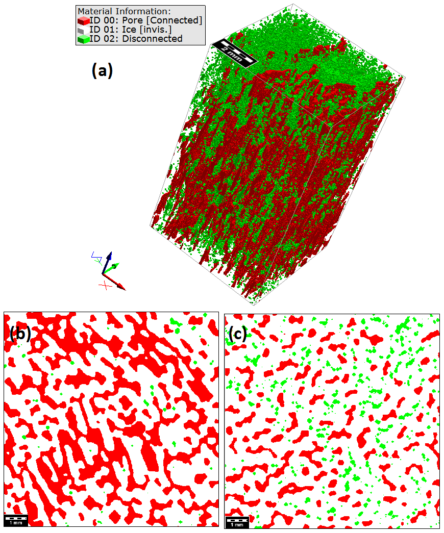
Figure 5XRT micro-tomographic images illustrating the open (red) pores and closed (green) brine pores in young sea ice. (a) 3D image, ice being invisible; (b) horizontal section from the 3D image with open pores dominating, ice being white; (c) horizontal section from the 3D image with a similar fraction of open and closed pores. The 2D scale bar is 1 mm; the side length is 10.8 mm.
The horizontal slices are taken from two different regimes of this image, one with predominately connected (Fig. 5b) and one with a similar fraction of connected and disconnected pores (Fig. 5c). In the predominately connected pores (Fig. 5b), one observes a high degree of horizontal connectivity. The patterns appear well resolved by the present voxel size (of 18 µm). One also can see that there are many bottlenecks (or throats) in the horizontal connectivity, and one can identify some green spots, where inclusion shave pinched off. In Fig. 5c with many more disconnected inclusions, the overall connected-pore width is smaller, and the horizontal connectivity is low. Note however that the red pores are still connected to one of the sides of Fig. 5a.
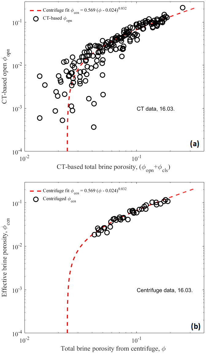
Figure 6(a) Relationship between CT-based open brine porosity ϕopn and CT-based total brine porosity (ϕopn+ϕcls), shown as circles, in comparison to the centrifuge-based effective porosity fit (dashed red curves). (b) The relationship between ϕcen and ϕ for the same ice core samples (a 5-core subset of the 15 ice cores in Fig. 4a). Note that (a) shows results for sub-samples of the samples in (b).
In Fig. 6a we plot the CT-based open brine porosity ϕopn against the CT-based total brine porosity (ϕopn+ϕcls) for all samples and compare them to the centrifuge relationship between ϕcen and ϕ. Figure 6b shows the corresponding centrifuge data for the same five ice cores and sampling day, also on a double-logarithmic scale (note that Fig. 4 and the optimal fit were based on all 15 ice cores from the three sampling dates). It is obvious that the smaller CT samples extend the range from the centrifuge data to lower ϕ and ϕopn compared to ϕcen.
Above a total porosity of ϕ≈0.05 the CT-based open porosity agrees well with the ϕeff(ϕ) relationship obtained by centrifugation. At lower porosities the CT data still follow the relationship reasonably well, in support of the deduced threshold ϕc=0.024, yet become more scattered. Note that each CT data point represents for a cm3 sub-sample roughly of the volume of the centrifuged samples. The scatter may thus be related to centimetre scale internal variability. On the other hand, the scatter may be due to segmentation errors for both ϕopn and ϕcls that at low porosities may reach 100%.
3.2.3 Centrifuge-based open-porosity conversion
The CT-image-based permeability and pore sizes to be presented in the following paragraphs could be correlated to different porosity metrics – the centrifuge effective porosity ϕcen, the centrifuge-based total porosity ϕ, the CT-based effective and open ϕopn, and the CT-based total brine porosity (ϕopn+ϕcls). To make a comparison to other studies and a general application feasible, the total brine porosity is chosen. However, permeability will depend on the CT-based open porosity ϕopn or more accurately the connected porosity ϕzz. The CT porosities in Fig. 6a are scattered, and we cannot say to what degree this is due to segmentation errors, small undetected brine inclusions and/or redistribution during cooling of the centrifuged sample, in particular for ϕcls. We thus make the following approach. We replace the centrifuged porosity ϕcen in Eq. (6) with ϕopn to obtain a CT-based total porosity ϕ. Hence, all data in Fig. 6a are mapped onto the dashed red curve. In this way we preserve the essential property information to which the permeability relates, the open porosity ϕopn, but present all data in terms of a total brine porosity ϕ that is computed from ϕopn.
3.3 Permeability
The results of the permeability simulations for all sub-samples are shown in Fig. 7 in relation to the total brine porosity ϕ (converted from ϕopn). As noted, this conversion incorporates the percolation threshold ϕc=0.024 deduced from the centrifugation into the analysis. The simulations span a permeability range from to m2. The porosity regime 0.024 to 0.33 above the percolation threshold is shown with grey shading. In this regime we also found impermeable samples.
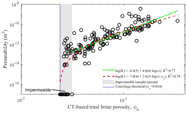
Figure 7Relationship of simulated vertical permeability K and the total brine porosity ϕ. Two log–log fits are drawn and specified in the legend, corresponding to power laws of the form K=a(ϕ)b (green curve) and (red curve). The numbers in brackets are the uncertainties in the last decimal of the log–log least-squares fit. The grey shading indicates the regime where permeable and impermeable samples are found.
We obtain two relationships between permeability K and total brine porosity ϕ by double-logarithmic least-squares fitting. Due to the extreme values we use the robustfit.m MATLAB function that gives less weight to outliers. Also, only the data with ϕ>0.031 were fitted, that is the regime where no impermeable samples are found. The first relation is a simple power law as most frequently used in sea ice studies involving the permeability:
The 95 % significance bounds are a factor of 100.5 for the pre-factor and 0.4 for the exponent (Fig. 7). The second is a percolation-based relationship between K and (ϕ−ϕc)
Also here, only the data with ϕ>0.031 were fitted, though the relationship is shown for the whole regime to illustrate the percolation behaviour. The 95 % significance bounds are here a factor of 100.4 for the pre-factor and 0.3 for the exponent. The R2 of both fits is almost the same. However, Eq. (7) does not account for the transition to impermeable samples at low porosities.
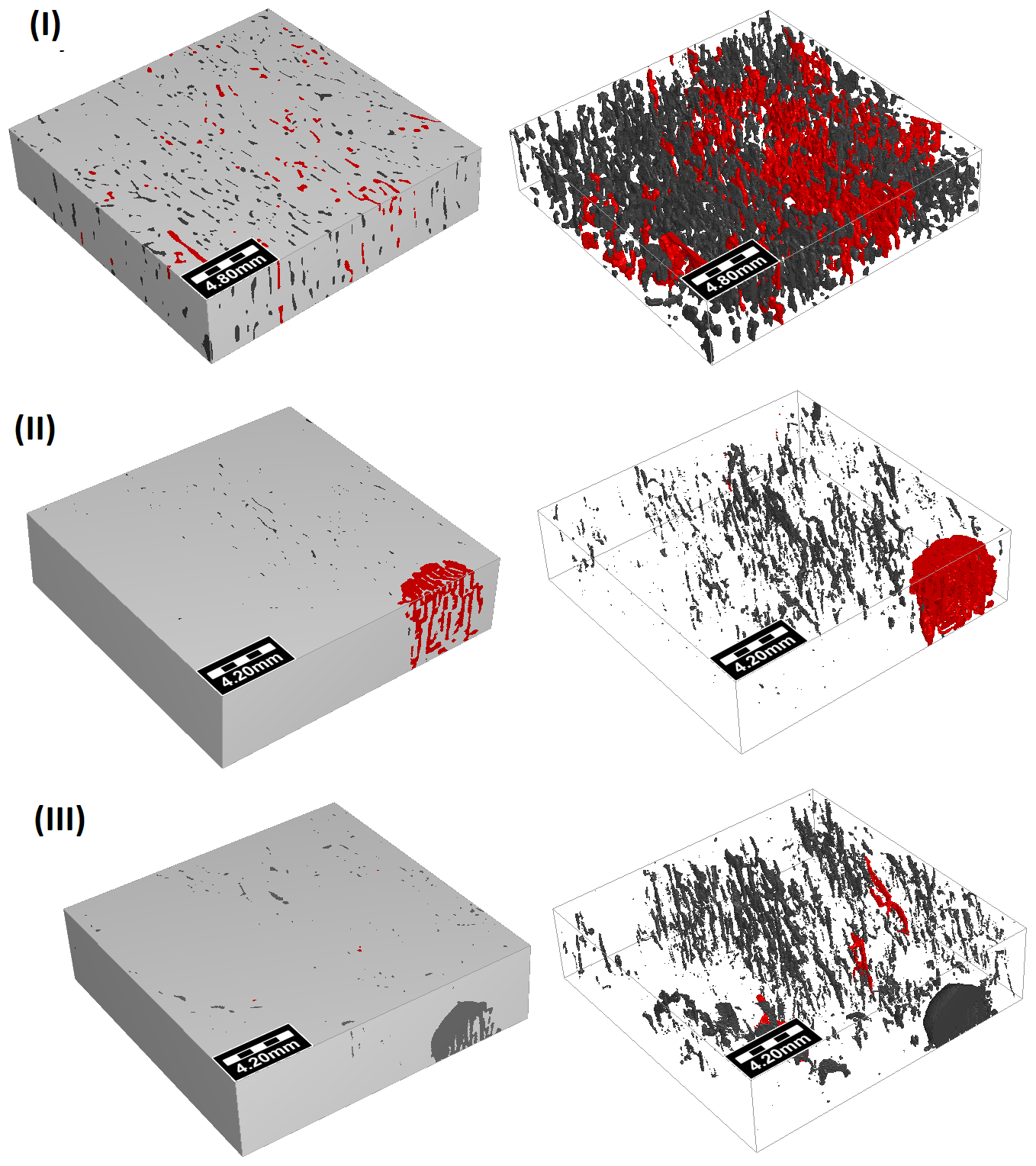
Figure 83D images of typical samples as discussed in the text. The left images are 3D images emphasizing the pores visible at lateral boundaries; the corresponding right images show the pore space with ice being invisible, focusing on the sample interior. Vertically connected pores, contributing to the permeability, are shown in red; other pores are shown in dark grey; and ice is shown in light grey. (I) Only small pores, half of which are connected; (II) one connected large pore, no small ones; (III) a few connected small pores and one unconnected large pore running out laterally.
At a given porosity the permeability can typically vary over 2 orders of magnitude. There are, however, a couple of data points with larger deviation. Figure 8 illustrates the different microstructures to which this behaviour is related. Three examples of sample types have been selected: type (I) is the most frequent sample type of young ice, with many parallel vertically oriented layers of pores and inclusions. The vertically connected pores are distributed over the whole sample (with total ϕ≈10 %). The computed permeability ( m2) is close to the least-squares fits. Type (II) is a sample type with a rather localized concentration of vertically connected parallel layers and pores. The example has a total brine porosity (ϕ≈3.3 %) slightly above the percolation threshold, and the computed permeability ( m2) is 2 orders of magnitude above the fitted relations. Type (III) is a sample type with very low brine fraction of connected pores (ϕzz≈0.06 %). The example has a total brine porosity ϕ≈3.4 % slightly above the percolation threshold, and the computed permeability ( m2) closely follows the least-squares fit.
3.3.1 Connected porosity and tortuosity
According to Eq. (5) the permeability simulations are related to two additional properties. The first is the connected porosity ϕzz, the second the tortuosity τ of the flow across the sample. For finite-size images these may be related in the following way: if the tortuosity approaches or becomes larger than the sample size, then ϕzz will decrease because channels will hit the lateral boundaries. Both properties are therefore investigated in Fig. 9a and b.
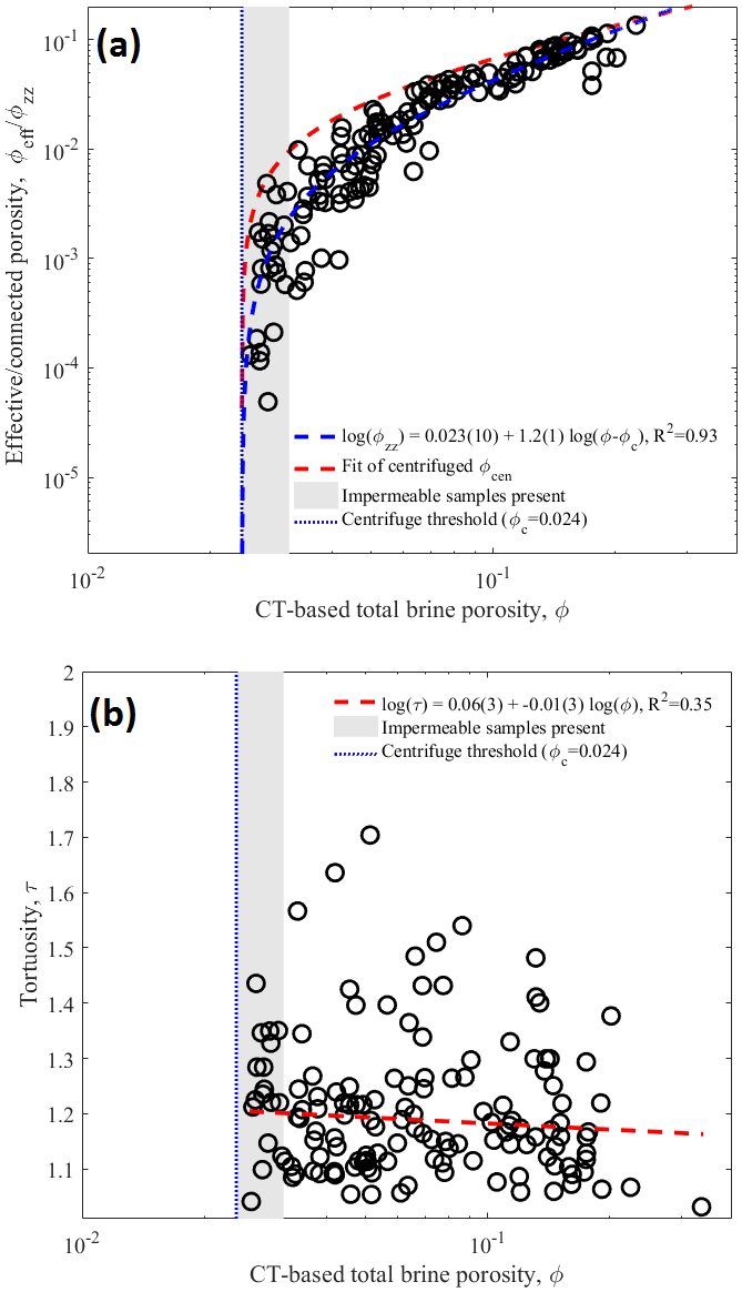
Figure 9(a) Relationship between CT-based connected porosity ϕzz and total brine porosity in comparison to the centrifuge-based fit of the open porosity ϕcen. (b) Tortuosity of the flow based on the length of the path of the channel with maximum diameter.
Also for the connected porosity in Fig. 9a we obtain a double-logarithmic fit of the form and find an exponent that is larger than the exponent 0.83±0.03. Comparing the fits in the figure shows that ϕzz is consistently bounded from above by ϕcen.
The tortuosity shown in Fig. 9b is simply the ratio of the length of the maximum diameter path Lpth and the sample thickness L. For this property no measurable change with porosity is observed, indicating that its influence on the permeability can be considered to be small.
3.4 Characteristic pore scales
Average pore size distributions of our data are shown in Fig. 10, emphasizing the pore size change during cooling. The left-hand figure shows results for open brine pores. The distribution for the two warmest cores with temperature −2 to −4 ∘C in Fig. 3 is shown with red bars, the distribution for the two coldest cores with temperatures −6 to −10 ∘C with blue bars. The corresponding cumulative distributions are shown as dashed (warm) and dotted (cold) lines. The left y axis refers to the bars and gives the fraction of open pores in each size class, while the right-hand y axis refers to the cumulative fraction. It is seen that, for the warm and cold sample populations, more than 95 % of the pores have a diameter of less than 1 mm. Relative changes due to temperature are largest below 0.4 mm. The median of the open-pore diameter, given by the fraction 0.5 in the cumulative distribution, changes from 0.20 mm for the warm ice to 0.16 mm for the cold ice. Note that the distribution for both warm and cold ice has two modes, one near 0.15 mm and another one near 0.10 mm. The throat size distribution is similar to the open-brine-pore distribution with slightly smaller median values of 0.14 and 0.10 mm for the warm and cold ice cores and modes near 0.14 and 0.08 mm.
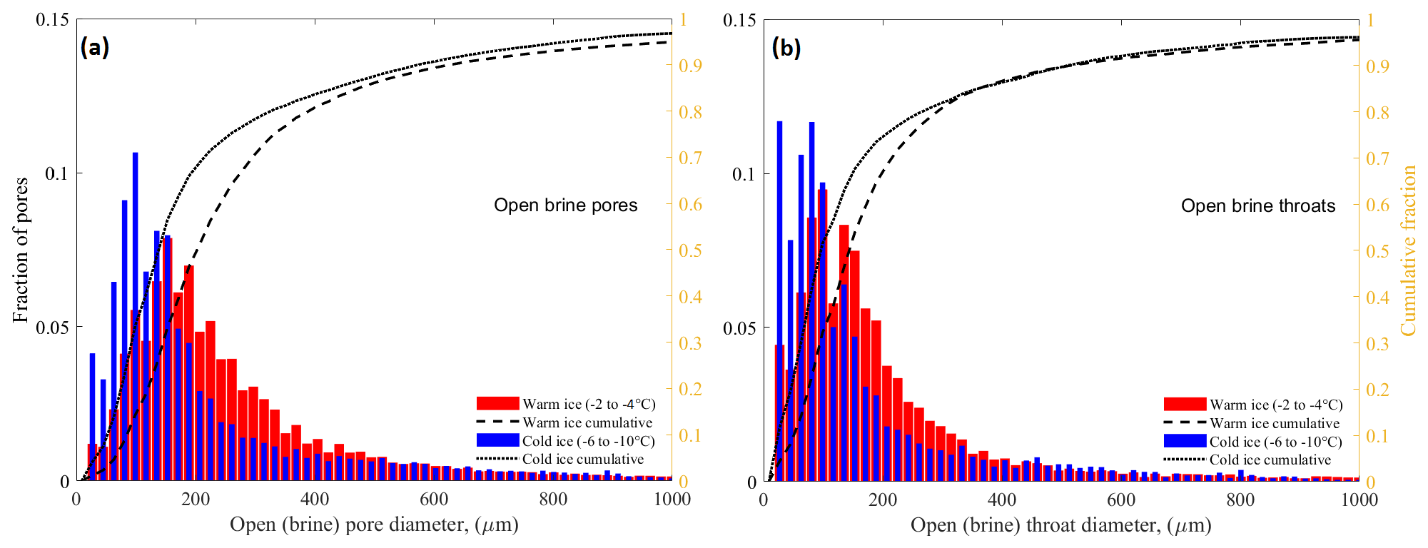
Figure 10Pore size distributions based on XRT imaging of four young ice cores. (a) Fraction of open brine pores in 18 µm wide size bins for the two warmest (red) and two coldest (blue) cores. The corresponding cumulative fractions are also shown with the y axis on the right-hand side; (b) same as (a) but for the porosimetry and fraction of pores throats.

Figure 11Characteristic pore scales and their dependence on brine porosity. (a) Median open-pore size Dopn; (b) median throat size Dthr; (c) pore scale based on specific surface area Dssa; (d) maximum path diameter Dpth. For all length scales a power law D∼ϕd has been determined by double-logarithmic least-squares fit, shown as a dashed red line. The fit is given in the legend, with numbers in brackets giving the uncertainties in the last decimal. For Dssa the fit is only based on data with ϕ>0.031, outside the regime where impermeable samples are found. The critical pore scales are obtained where the dashed red lines cut the percolation threshold ϕc=0.024. The Nyquist criterion (2× voxel size) is shown as a horizontal green line.
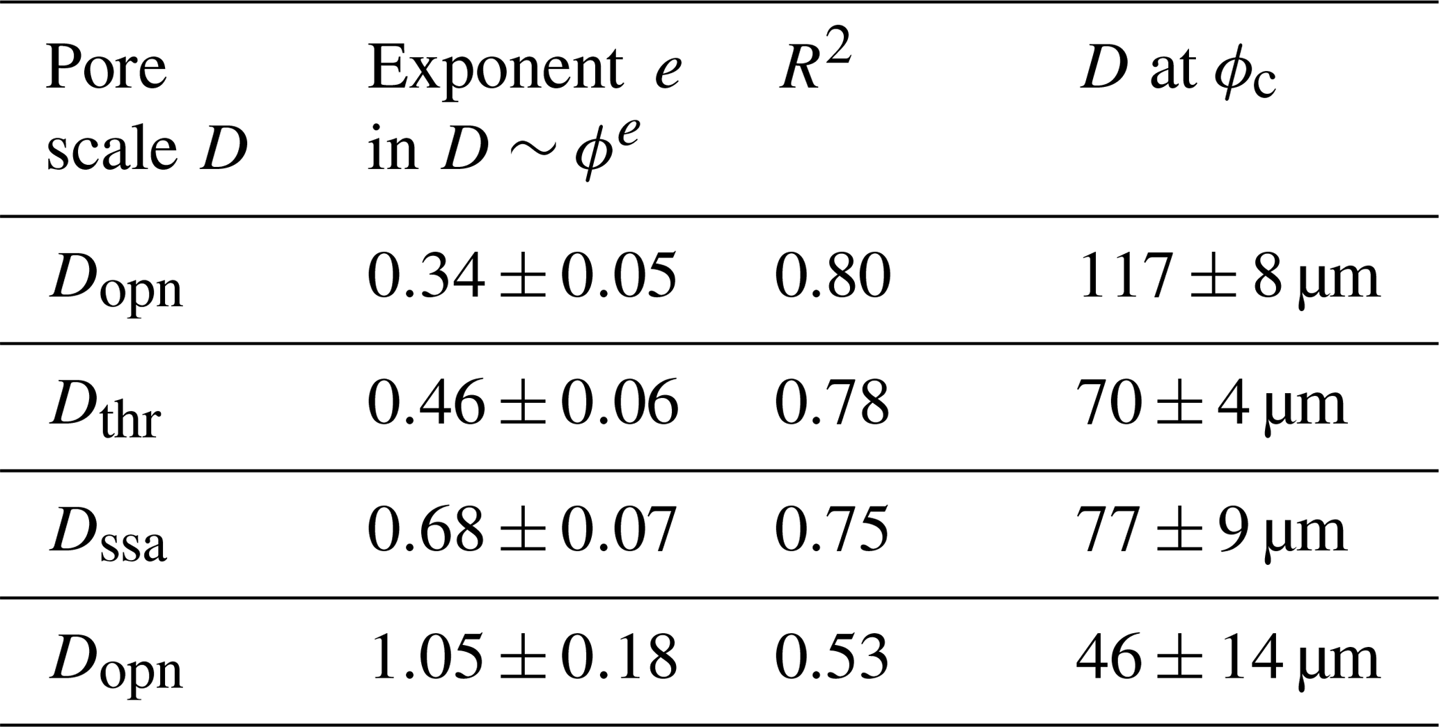
Due to variability also in pore scales, the pore size characteristic scales have been determined as median rather than mean values of the volumetric pore size distribution. Figure 11a to d show their dependence on brine porosity and that all pore sizes are increasing with ϕ. This increase has been evaluated by a robust double-logarithmic least-squares fit in order to obtain the power law behaviour of the form D∼ϕe. This relationship is indicated in the figures. Also shown is the transition regime for which both permeable and impermeable samples have been observed, with grey shading, and a number indicates which scale the fitted power law has reached at the percolation limit of ϕc=0.024. A horizontal green line marks the length scale of 2 voxels (36 µm) that often is considered to be the Nyquist criterion of digital imaging, which states that the sampling interval has to be at least twice the highest spatial frequency to accurately preserve the spatial resolution. This is of particular importance in our study for identification of channels with a path through the sample. A path of just 1 voxel width would very likely be terminated at some level.
The results for the open-pore size Dopn are shown in Fig. 11a. Despite a few outliers, weighted less in the robust fit applied, there is a well-defined relationship with a linear slope in log–log space and Dopn∼ϕ0.34, with R2=0.80. Near the percolation threshold a few lower values are seen to drop below the fit.
The results for the throat size Dthr are shown in Fig. 11b. They follow in principal the behaviour of the open-pore size Dopn, yet being typically 1.2–1.7 times smaller and with a slightly steeper slope Dthr∼ϕ0.46. Also the throat size shows a drop of a few samples close to the percolation threshold.
The specific-surface-area-based length scale Dssa is shown in Fig. 11c. Here, a linear fit in log–log space obviously does not work for porosities smaller than 0.03, and the grey shaded transition regime has thus been excluded from the fit. The transition of Dssa to lower values than the least-squares fit (related to larger specific surface) starts at higher porosity than for Dopn and Dthr. That values drop below the proposed resolution limit is related to an algorithm in GeoDict employing estimates of specific surface more complex than a simple sphere-fitting approach.
The last length scale to be considered is the maximum path diameter Dpth, corresponding to the maximum diameter of a sphere that can permeate through the sample. Dpth is thus based on an approach comparable to the throat size Dthr. The values are much more scattered than Dthr, and their relationship with ϕ has a larger slope with Dpth∼ϕ1.05, though with less confidence than for the other length scales. It is seen that the lowest values of Dpth are close to the resolution limit line below a porosity of ϕ<0.05.
The exponents of the pore scale versus brine porosity relationships as well as the pore sizes at the threshold porosity ϕc=0.024 are summarized in Table 3.
We have obtained results for the permeability and pore scales of sea ice through a challenging procedure with the following steps: (i) field sampling of a large number of cores (15) of uniform ice, (ii) thorough temperature control of samples at in situ values, (iii) centrifuging samples at in situ temperatures, (iv) X-ray micro-tomographic imaging, (v) pore size analysis and numerical permeability simulations. Also, by lowering the temperatures of harvested ice cores in the lab, we extended the original in situ temperature regime of the samples (minimum −3 ∘C) down to −10 ∘C and obtained results for brine porosities down to ϕ≈0.03.
It needs to be pointed out that the centrifugation approach has been essential to obtain the XRT results. XRT imaging, the method of choice for non-invasive imaging of the internal structure of materials (Kinney and Nichols, 1992; Buffiere et al., 2010), is these days increasingly used in the geosciences (Cnudde and Boone, 2013). It has become an important method in snow research (Flin et al., 2004; Schneebeli and Sokratov, 2004; Heggli et al., 2011), and recent work has indicated its potential for sea ice microstructure analysis (Golden et al., 2007; Pringle et al., 2009; Obbard et al., 2009; Maus et al., 2015; Crabeck et al., 2016; Lieb-Lappen et al., 2017). However a limitation for application to sea ice stems from the small X-ray absorption contrast between ice and (sea)water (Bartels-Rausch et al., 2014). Imaging sea ice at lower temperatures than in the field gives, due to the corresponding higher salinity of brine, reasonable contrast (Obbard et al., 2009; Lieb-Lappen et al., 2017), yet pore sizes and connectivity will differ from in situ conditions (as clearly shown in the results presented here). XRT imaging has thus been performed on ice grown from salt water with CsCl added as a contrast agent (Golden et al., 2007; Pringle et al., 2009). Such “doping” is not feasible in the field. In the present work, to solve the contrast problem and obtain good images of relatively warm sea ice, the ice samples were thus centrifuged prior to imaging, replacing brine with air with much higher contrast to ice (Weissenberger et al., 1992; Maus et al., 2011, 2015).
4.1 Effective versus total porosity
Centrifuging is not only a means of obtaining high-quality XRT microstructure images. It provides the dependence of centrifuged (effective) porosity on total brine porosity as well as a porosity threshold of %. This threshold is a new result compared to most earlier work that has more or less accepted a value of 5 % (e.g. Golden et al., 1998; Cox and Weeks, 1988; Petrich et al., 2006; Golden et al., 2007; Pringle et al., 2009), which is further analysed below. The derived empirical relationship between effective and total brine porosity (Eq. 6) should be relevant for model applications that need to know the effective porosity. The deduced critical exponent 0.83±0.03 is of relevance for model approaches based on percolation theory. In terms of the latter, ϕcen can be interpreted as the probability of belonging to the infinitely connected cluster. So far sea ice permeability has been studied in terms of isotropic percolation (Petrich et al., 2006; Golden et al., 2007; Pringle et al., 2009), for which the critical exponent for the infinite-cluster strength is known to be β≈0.41 in 3D (Stauffer and Aharony, 1992; Sahimi, 1993). However, in sea ice the growth, pore structure evolution and desalination processes are anisotropic and directed towards the ocean. For such a setting, typical for many natural porous media, Broadbent and Hammersley (1957) have already suggested that the percolation should be directed. Directed percolation belongs to a different universality class with critical exponents differing from the isotropic case, β≃0.82 being the presently accepted value for β in three (plus one, the direction) dimensions (Henkel et al., 2008; Hinrichsen, 2009). Our deduced is in close agreement with the latter. On the one hand this gives us strong confidence for the validity of the centrifugation approach and its results. On the other hand it points to the need to analyse sea ice in terms of directed rather than isotropic percolation; e.g. it will be a future challenge to study the anisotropy in permeability observed by Freitag (1999) and the directional dependence of the porosity threshold found by Pringle et al. (2009) in terms of directed percolation.
We have considered and avoided several possibilities how centrifugation might bias the results. Incomplete centrifugation of brine might lead to brine remnants which, after cooling and freezing, might block pores (Freitag, 1999). This might create a higher apparent porosity threshold, indicated by an earlier study (Buettner, 2011) with lower centrifuge acceleration (15 g compared to our 40 g). By carefully choosing the parameters we think that we largely avoided this problem. Also the warming of ice samples in the centrifuge was carefully tested and avoided by using a centrifuge start temperature 1 K below the in situ sea ice value. Other effects, like pressure melting of ice or internal deformation, are unlikely at the relatively small centrifuge acceleration rates we used. We cannot exclude that centrifuging has implied minor deviations from in situ temperatures. However, what we derive, in essence and for the first time, from centrifuging and CT imaging is the relationship between open porosity, total porosity and permeability. We rate it as unlikely that small internal structure changes due to fluid redistribution and freezing and melting in the centrifuge will change this relationship fundamentally.
4.2 Effective versus connected porosity
The comparison of CT-based connected porosity ϕzz to open porosity ϕopn in Fig. 9a indicates that vertically connected and open porosities become more different when the total porosity decreases. The exponent in is compared to the exponent 0.83±0.03 for the open and centrifuged porosity.
We can obtain a simple estimate of the fraction of brine channels that can be expected to open to the sides and not contribute to ϕzz. Assuming a simple 2D geometry and that all pores are parallel, this fraction will be approximately tan (α)ϵ, where α is the inclination angle of crystals and channels against the vertical and ϵ the ratio of sample height to diameter. For sea ice a typical has been documented (Kovacs and Morey, 1978; Langhorne and Robinson, 1986; Kawamura, 1988). Freitag (1999) has performed a sensitivity test and found a permeability reduction with sample height that was consistent with . For our , the effect is an underestimate by less than 5 %. In the standard experiments from Freitag (1999), with , one would expect a slightly larger underestimate of 12 %.
From this consideration we conclude that the inclination of crystals alone cannot explain the increasing difference between ϕzz and open porosity ϕopn. A pore splitting mechanism that disconnects vertical pores that are still connected to the lateral sides must be operating, contributing to ϕopn and not ϕzz.
4.3 Pore size threshold
In Fig. 11a to d we show that all characteristic length scales decrease with decreasing porosity. For two length scales, the median open-pore size Dopn and the median throat size Dthr, very robust power law relationships of type D∼ϕd were obtained. These relationships do not show percolation behaviour of the form , but they are supposed to create the percolation behaviour in ϕzz and ϕopn as follows. By evaluating the power law relationships at the present percolation threshold ϕc, we obtain their critical values at the percolation threshold. Of particular interest is the critical throat diameter
at the threshold. We interpret it as the throat diameter at which necking occurs to lock the brine pores.
This result is consistent with two earlier studies of sea ice microstructure. Anderson and Weeks (1958) discussed the transition from brine layers into cylindrical brine tubes in connection with changes in the relationship between sea ice strength and brine porosity. They proposed, based on an analysis of horizontal thin sections, a splitting of layers into channels near a tube diameter of 0.07 mm. These authors have not presented a statistical analysis of their results but mention that they obtained the value from “photographs of layers just before and after the splitting”. From the plate spacing reported for their study (0.46 mm on average) it may be suspected that they analysed mostly young ice of similar age as ours. The agreement of our and their result is very interesting. Also Light et al. (2003) studied the temperature dependence of sea ice microstructure in order to formulate a model for the radiative properties of sea ice. Based on the optical analysis of many samples, they distinguished morphologically between brine tubes (above a length of 0.5 mm) and brine pockets (below this value) and derived an equation for the aspect ratio (length L divided by diameter D) of tubes and pockets (10.3D=L0.33). Inserting the pocket–tube transition of 0.5 mm for L one obtains a tube diameter of 0.077 mm at the transition, indicating also here a similar scale for the splitting of tubes.
The critical median open-pore size Dopn,c computed at the threshold was 117 µm, a factor of 1.7 larger than Dthr,c. This is likely the value that one would identify by considering all pores in a thin 2D section because one would not know which the throats are. Also noteworthy, though not investigating the temperature dependence or transition from pockets to tubes, is the study by Cole and Shapiro (1998) of Arctic first-year ice at the start, middle and end of the freezing season. These authors were not simply doing thin 2D sections but sectioned sea ice vertically and horizontally to obtain the dimensions of brine filaments in three directions (their Fig. 9). They found the average width of brine inclusions, at a depth of 0.2 m, to increase from 0.08±0.03 mm to 0.14±0.04 mm (their Fig. 10b). The imaging temperature was −14 ∘C, which, with the reported salinities of 5–7 psu, indicates a porosity of 0.022 to 0.031. This condition is similar to the percolation limit in our study, which is supported by the fact that Cole and Shapiro (1998) indeed mostly observed vertically disconnected brine filaments. The range of observed brine inclusion widths is consistent with our median open-pore size Dopn,c. Perovich and Gow (1996) have also optically analysed sea ice inclusions in thin 2D sections, focusing however on other microstructure characteristics. From their tabulated values of major axis length, perimeter and circularity of ellipses that were fitted to brine pores, one can deduce a minimum axis length. Median values obtained in this way (see Maus, 2007) fall in the range of 0.05 to 0.1 mm and are comparable to our observed values. However, from the 2D data no information on pore connectivity and necking is available.
The analysis of pore and throat diameters thus gives us important information about the critical length scales at the percolation transition. More supporting information comes from the specific surface area length scale that we compute by assuming that the surface area relates to infinite pores with circular cross-section, which means . This is the only length scale that appears to show critical behaviour near the percolation threshold. This behaviour indeed supports the necking hypothesis as follows: consider a long brine pore that splits into spherical inclusions. While Dopn and Dthr will not change much, the SSA does increase during the transition to spheres. However, to account for this in the length scale computation one would have to calculate . As this is not done for the data points in Fig. 11c, there is an apparent drop in our computed Dssa when splitting takes place, nicely seen in our data.
But we can, through Dssa, not only identify the necking and splitting near the percolation threshold. When considering that the power law fits D∼ϕd, one would expect that, if decreasing DSSA with ϕ would only relate to diameter changes, it should be described by a similar exponent d as Dopn (0.34±0.05) and Dthr (0.046±0.06). However, if the fit is also restricted to the regime ϕ>0.031, we find an exponent (equivalent to the slope in log–log space) that is larger for Dssa (0.68±0.07). The interpretation is that splitting and necking operates over the whole porosity regime in our dataset.
The critical value of mm should probably be interpreted as a statistical descriptor of the pore space rather than a strict limit. Looking at the fourth characteristic length scale, the maximum path diameter Dpth in Fig. 11d, we see that there exist throughflow paths with lower diameter. This is not unexpected in the sense that the throat size distribution only has its median at 70 µm at the transition. Another approach to estimate the critical Dthr,c is based on the following argument. Cooling ice does decrease the brine volume and leads to shrinking of pores and, for a range of ice temperatures, to a broad distribution of pore sizes. If however there is a preferred pore size for necking, then pores will not shrink around this value as internal freezing now rather closes pores. Hence, one would expect a local maximum in the pore size distribution. A look at average throat size distribution in Fig. 10b indeed shows such a maximum. For the cold ice (blue bars) it is located near 0.08 mm (in the size class 72 to 90 µm) and hence consistent with the result from the least-squares fit. For a more detailed discussion the present dataset is somewhat limited here as the lower range of the identified maximum path diameters touches the Nyquist spatial criterion of 36 µm below a porosity of 0.05. Figure 11d indicates that, to study the necking transition near the percolation threshold dynamically, one would likely have to increase the present resolution by at least a factor of 2.
Regarding the mechanism of necking, Anderson and Weeks (1958) had once argued that the necking of pores is driven by surface energy effects. However, one of us has argued that (i) the original brine layers are expected to be low-energy surfaces and that (ii) latent heat energy fluxes during freezing are many orders of magnitude larger than surface energy transitions (Maus, 2007). Due to these factors it seems more likely that morphological freezing instabilities in supercooled brine layers and pores play a role for the necking in a similar way as they do for the plate or brine layer spacing at the ice–water interface (Wettlaufer, 1992; Maus, 2020). A concise physical explanation for the necking phenomenon is lacking so far. Progress could be made by direct observations of the 3D pore space evolution by X-ray tomography, building on 2D visual observations of pore necking described by Niedrauer and Martin (1979) for a thin growth cell. Such an approach may be feasible through fast-time-lapse synchrotron-based X-ray tomography for low-contrast materials (e.g. Beckmann et al., 2007; Buffiere et al., 2010). Conventional laboratory-based XRT with higher spatio-temporal resolution may also provide new insight into the details of necking and pore instabilities.
4.4 Permeability
Having found consistent explanations of the observed percolation limit in terms of critical pore sizes, we now return to the permeability simulations. In Fig. 12 we compare our results to the results of two experimental studies on young ice.
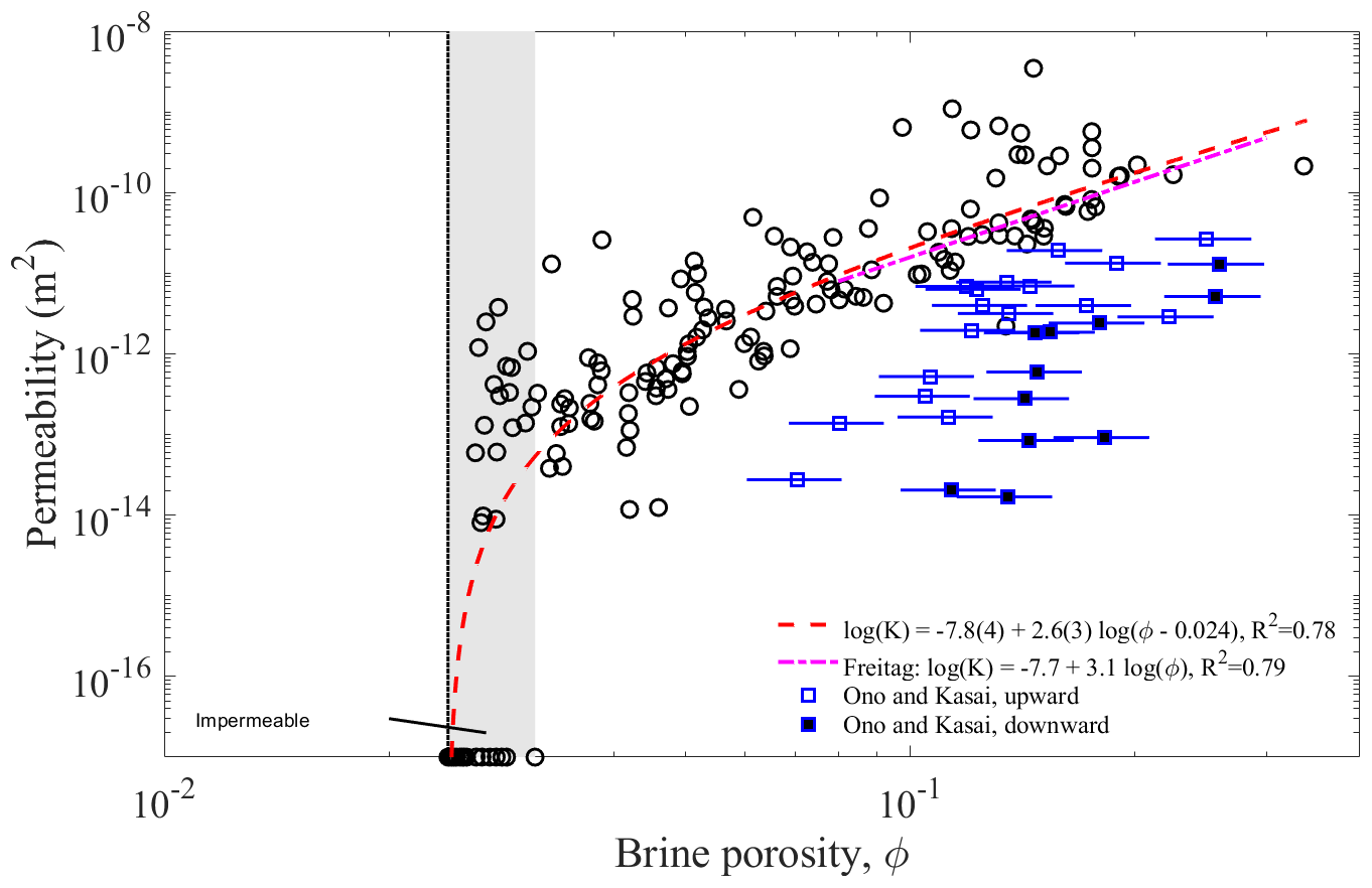
Figure 12Relationship of simulated vertical permeability K and ϕ−ϕc as shown in Fig. 7 as a dashed red curve, here compared to two earlier investigations. As the measurements from Freitag (1999) are only available in terms of ϕcen, we plot the least-squares fit from Freitag (cyan curve, numbers given in the legend). The data points from Ono and Kasai (1985) represent downward and upward permeation of brine through the ice; see text for more information.
The relationship based on the work by Freitag (1999) is likely the most frequently cited and used in the literature. Freitag only documented the data points of K versus the centrifuged brine porosity ϕcen, yet he has given the relationship between K and total brine porosity ϕ. It is given in the legend of Fig. 12 and plotted as a dashed green curve. The porosity range for Freitag's fit () has been estimated from the ϕcen values he reported. Comparison with our fit (the dashed red curve) indicates a very good agreement with Freitag's results for his porosity range of validity. The maximum difference is just 30 %. As the confidence bounds for our fit indicate roughly a factor of 2, there is no significant difference in the predictions. However, our relationship is based on a fit of observations down to ϕ=0.03 and allows the estimation of permeabilities at low porosities, where Freitag's relationship is not applicable.
The second dataset is from experiments that Ono and Kasai (1985) performed with artificially grown young ice. These authors did not publish the permeability but rather the hydraulic conductivity, and we have used Eq. (3) to convert from to permeability K. To do so we used the temperature- and brine-salinity-dependent kinematic viscosity relationship from Maus (2007). As Ono and Kasai only reported surface temperatures of their tested ice, we make the assumption that the salinity is similar to those reported for ice growth experiments from other laboratory studies. For the documented ice growth velocity of 10−4 cm/s and water salinity (Sw≈33 ‰ NaCl), a 6 cm thick sea ice crust will typically contain 40 % to 50 % of the salinity of water from which it grows (Wakatsuchi, 1974, 1983). We thus assume a sea ice salinity of ‰ NaCl. We shall use this range with reported surface temperatures to estimate the brine volume ϕ at the surface of the ice. This leads to the blue data points and uncertainty estimates in Fig. 12. There are two sets of data. The open squares are based on measurements of upward movement, where Ono and Kasai created a pressure gradient directed from the water into the ice. The filled squares are based on measurements of downward movement where the authors poured brine, in salinity equilibrium with the surface temperature, onto the ice. The surface temperature was adjusted with an infrared lamp.
It is seen that the permeability data from Ono and Kasai (1985) fall 1–2 orders of magnitude below our and Freitag's observations. The error bounds indicate that this hardly can be explained by a lower salinity of freshly grown ice (at 10−4 cm/s) than assumed. We think that the difference is related to two factors. The first is related to the fact that, in contrast to our and Freitag's study of sub-sample permeability, Ono and Kasai measured the permeability of the full ice thickness (of however only 6 cm). In this setting the ice surface, where the ice is coldest, will control the permeability. However, in most cases the first surface ice skim is growing much faster, implying smaller crystals (or plate spacing) and thus more tiny pores between them, with a strong impact on the permeability (e.g. Okada et al., 1999). In addition to crystal size, a more random crystal orientation may imply tortuous flow and decrease the permeability further. The second factor is likely related to changes in the microstructure during the experiments, also discussed by Freitag (1999). Assume that the upward flow experiments were performed first. As during the flow less saline seawater is exchanged for brine, the ice salinity will decrease. At high surface temperatures (similar to those in the seawater) this salinity decrease is low, yet it becomes large with the temperature difference between the ice surface and the water. This is consistent with larger deviations in the data points from Ono and Kasai from our permeability fit at lower brine porosity. If the downward flow experiments were then to take place after the upward flow, salinities could have been considerably less than assumed for freshly grown ice. The argument also works vice versa to explain the difference in the upward and downward results as during downward flow of high-salinity brine the bulk salinity of an ice sample is expected to increase. Based on these arguments, the data from Ono and Kasai (1985) provide some qualitative support for the existence of a sharp transition in permeability at some critical brine volume fraction or temperature, as proposed by Golden et al. (1998). However, the nature of their experiment was not suited to validate such a brine volume threshold quantitatively.
We recall that the double-logarithmic fit in Fig. 12 is only based on our data above ϕ=0.031, excluding the regime where we find permeable and impermeable samples. The investigation of the characteristic pore scales, in particular the maximum path diameter shown in Fig. 11d, also indicates that we start facing resolution problems below a brine porosity of ϕ≈0.04. This, as well as image segmentation errors, may to some degree explain that the data points in the regime appear significantly above our proposed relationship. And one can argue that some kind of averaging of zero permeabilities with these high values would move the data closer to the fitted percolation curve. As our data in this regime are not of high enough quality, we have not applied such a correction. However, the combination of good enough image quality above ϕ≈0.04 has, in combination with the threshold ϕc=0.024 from the centrifuge experiments, enabled us to deduce Eq. (8) with good confidence, at the same time being consistent with the work of Freitag (1999).
Over the whole range of porosities, we find some samples with permeabilities 2 orders of magnitude larger than the fitted curve and most data points. As discussed above these are associated with type (II) ice samples in Fig. 8 and the presence of larger brine channels. Such a dual system of pore sizes is a frequently described but in detail still little explored feature of sea ice (e.g. Wakatsuchi, 1983; Wettlaufer et al., 1997; Weeks, 2010; Rees Jones and Grae Worster, 2014). That only part of our samples do contain larger brine channels is likely related to our limited sample size (3 cm diameter resulting in 2 cm side length for numerical simulations), in turn leading to the scatter in permeabilities. However, the large number of samples and the additional constraint ϕc=0.024 from centrifuging larger samples has allowed us to obtain a statistically robust relationship between K and ϕ. Yet the uncertainty is still a factor of 2. Improvements may be made on the basis of currently available X-ray detectors that allow for a 2 times larger field of view (at the same spatial resolution), with a better representation of the dual brine pore size networks.
For modelling efforts of the permeability with porosity, the obtained exponents are of high relevance. In general the dependence of permeability K on porosity ϕ is often empirically characterized by an equation of the form K∼ϕb. The simplest model is to relate porosity ϕ to pore diameter d and assume the well-known relationship K∼ϕd2. From the basic sea ice microstructure of parallel brine layers (d∼ϕ) and circular tubes () one could argue for . The larger exponent that we find (Fig. 7) reflects that not only pore diameters are changing with porosity but also their connectivity. Percolation theory accounts for this effect, which resembles an equation that involves the threshold porosity in the form (see also Eq. 8). For isotropic percolation this has been first proposed as “critical path analysis” for the electrical conductivity (Ambegaokar et al., 1971), and the current best estimate for the conductivity exponent in the form is e=2.0 (Stauffer and Aharony, 1992). The permeability exponent t however will be larger than e=2.0 if the characteristic pore scale dc of permeating paths is changing with porosity. This problem has been addressed by several authors proposing an equation of the form ; e.g. Katz and Thompson (1986) proposed to determine the length scale dc on the basis of mercury porosimetry. This is indeed the approach (virtual porosimetry) we have applied to determine the throat sizes in the present study. If we insert the throat size exponent from Fig. 10b, dc∼ϕ0.46, and assume e=2.0, we would get a dependence of the form . This in turn is not very different from our percolation-based fit . We note that Golden et al. (2007) have proposed t=2.0 for older sea ice, arguing that wide brine channels with a constant critical diameter control the permeability, and also reported t=1.97 as a best fit to the data from Ono and Kasai (1985). We were unable to reproduce the latter result based on the data in Fig. 12, using our estimates of ice salinities in the experiments from Ono and Kasai (1985). Our best fit for the permeability critical exponent, , is largely consistent with percolation theory, critical path restriction by throats and their dependence on porosity. It is valid for young sea ice where the permeating pores are shrinking with decreasing porosity and will differ for ice with a different pore–porosity relationship. However, also for young ice a general prediction may be more complicated due to three aspects: first, it has been pointed out by Le Doussal (1989) that the approach from Katz and Thompson (1986) needs to be revised for broad pore size distribution, which may lead to higher exponents for the permeability. Second, the exponents may also be different for directed percolation. And third, ice type may play a role, and results for granular ice may be different. We are currently investigating this problem in more detail.
4.5 Porosity threshold
The present analysis has enabled us to deduce a porosity threshold of %. This optimal threshold cannot be deduced from the CT measurements alone as these data are scattered, and the CT samples are in volume of the centrifuged samples. However, the evidence based on the larger centrifuged samples is much stronger. Our confidence is related to the power law fit of the centrifuged porosity in Fig. 4 (critical exponent ) and its consistency with the theoretical critical exponent from directed percolation (critical exponent β≃0.82). Based on this agreement we can state that, if our hypothesis is correct that the pore space evolution of sea ice follows the behaviour of directed percolation, then this implies a threshold porosity for percolation in the range of 2 % to 3 %. The CT-based microstructure analysis supports these results and further can be interpreted in the way that the threshold is related to the necking or close-off of pores at a critical diameter of 0.07 mm. Our deduced porosity threshold is just half of the value of ϕc=5 % once proposed by Golden et al. (1998), which since then has been confirmed in other studies and become the most widely accepted threshold for sea ice permeability and desalination (Weeks, 2010). In the following we discuss these studies in the context of our results. The first proposal of a critical brine porosity and permeability of sea ice was once published by Golden et al. (1998). These authors proposed that sea ice typically becomes impermeable when its salinity is 5 ppt, its temperature −5 ∘C and its brine porosity 5 %, which is now known as the “rule of the fives”. To support this hypothesis the authors used a percolation model analogy of compressed powders, where the threshold depends on the ratio of critical brine inclusion to ice crystal thickness scales. As experimental evidence, the experiments from Cox and Weeks (1975) and Ono and Kasai (1985) discussed above were considered, indicating a porosity threshold of 5 % associated with a temperature −5 ∘C. However, on the one hand the model is simplistic and not backed up by detailed microstructure observations. On the other hand, our analysis above indicates that the experiments from Ono and Kasai (1985) are difficult to interpret. Assuming typical young ice salinities, the experimental data from Ono and Kasai (1985) would be far away from a porosity of ϕ≈5 %, while the suspected changes in ice salinity during the experiments are unknown. Due to these considerations and comparison to our simulations in Fig. 12, we think that the data points from Ono and Kasai (1985) cannot be used to qualitatively constrain a percolation threshold.
An earlier proposal of a critical brine porosity ϕc=5 % has once been suggested by Cox and Weeks (1988) based on observations of observed salt fluxes from sea ice (Cox and Weeks, 1975). The data have been later analysed in more detail by Petrich et al. (2006), coming to the conclusion that sea ice permeability is limited to brine porosities above ϕc≈5.4 %. However, there is a general problem with this argument: it is not the vertical permeability that has been observed by Cox and Weeks (1988) but the desalination of the ice. The latter however depends on other factors, like the brine salinity gradient in the ice and as well as the horizontal permeability to drive internal flow. The analysis may thus be interpreted to represent a porosity threshold at which convection sets in rather than at which the ice becomes impermeable.
The most stringent approach to estimate ϕc was proposed by Pringle et al. (2009) based on the first 3D analysis of CT images. These authors focused on the vertical connectivity ϕzz and investigated its scale dependence to estimate the connectivity threshold based on assumptions from isotropic percolation theory (Stauffer and Aharony, 1992). They investigated artificial cubic sea ice images with side lengths 2 to 7 mm. From the scale dependence of ϕzz they deduced a critical value of % for the vertical percolation threshold. This result thus seemed to support the earlier work and rule of the fives. However, in view of the present study and in particular the throat size threshold, this result may also need some revision. The critical aspect is that the detectability of pores was likely limited to widths of 83 µm (Nyquist criterion of 2 times the voxel size). In our study, with a 36 µm Nyquist criterion, we are observing larger scatter in connectivity and pore scales when the porosity threshold is approached. We thus suppose that such a problem may have influenced the percolation behaviour of the samples from Pringle et al. (2009) at 2 times coarser resolution; e.g. considering our deduced critical throat size of 70 µm, a similar value would not have been resolved by imagery with a 83 µm Nyquist criterion. A simplistic quantitative argument may be obtained by looking at Fig. 11b for the throat size Dthr and Fig. 11d for the maximum path diameter Dthr. We can ask at which porosity the lowest observed median throat sizes drop below 83 µm, which indeed happens in the range of %. Finally, though likely of minor importance, the results from Pringle et al. (2009) can be expected to change if critical exponents for directed rather than isotropic percolation, supported by the present study, would have been used in the derivation.
In summary, we interpret the earlier work as follows. The proposal of the rule of the fives by Golden et al. (1998) was based on measurements by Cox and Weeks (1975) showing that sea ice desalination due to gravity drainage almost vanishes for brine volumes below 5 % and on observations of the hydraulic conductivity of young ice (Ono and Kasai, 1985) showing large changes over a small temperature range. As the ice in the latter study likely had an initial porosity much larger than 5 %, and the data are difficult to interpret, they do not provide evidence for a 5 % percolation threshold. While an indirect approach by Petrich et al. (2006), also analysing the desalination data from Cox and Weeks (1975), supported a 5 % threshold, we point out that the latter study strictly only applies to the driving force of internal convection, not to the permeability itself. Last but not least, results from a CT-image-based study by Pringle et al. (2009) in support of ϕc of 5 % may have been resolution-limited (in view of the present higher-resolution results). Hence, many studies and datasets of young sea ice that have been proposed earlier in favour of a 5 % porosity threshold seem to require a revision, while our confident threshold range of 2 % to 3 % from centrifuging is a factor of 2 lower. We finally add a note to the question of whether the true threshold porosity might be even smaller and was limited by our centrifuge acceleration of 40 g. As discussed in connection with Eq. (4), we estimated that our settings should be valid to retrieve permeabilities as low as 10−14 m2. Hence, though we may have missed lower values, our overall data are consistent with percolation theory and the porosity threshold proposed here.
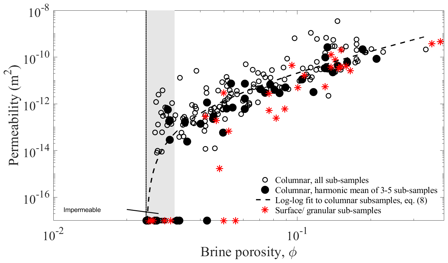
Figure 13Comparison of simulated vertical permeability K and ϕ−ϕc for columnar samples (as shown in Fig. 7 and here as open circles) to two other simulation results. The solid circles are harmonic means of all sub-samples (normally four to five) from each basic sample cut in the field (and centrifuged). The red stars are permeability results for near-surface samples (up to 5 cm from the surface) that were classified as granular ice and thus excluded from the basic analysis.
4.6 Other ice types and growth conditions
The discussion of earlier work and the present results apply to the permeability of young columnar sea ice during its growth phase, at a stage when mostly primary brine channels and pores exist. Here we discuss possible implications for other ice types, age, thickness and scale effects. We consider four aspects to be most relevant to generalize our results. These are dependence of permeability on (i) ice growth velocity, (ii) ice type and texture, (iii) ice age, and (iv) scale effects due to full-thickness finite sample sizes. The first three aspects are related to natural variability in growth conditions and thermal history. The fourth aspect is related to the process to be investigated (e.g. full-depth permeability for surface flooding versus near-bottom permeability for desalination or internal convection). It also relates to the question of whether tested samples are representative volume elements for the process and represent sea ice macrostructure.
- i.
Our range of 2 %–3 % for ϕc is valid for young ice that has grown at moderate growth rates (2–5 cm per day for both our and Freitag's experiments). We conjecture that this threshold is not a constant for sea ice but depends on growth conditions. The basic argument is that, if the critical length scale for necking of throats controls the transition, the critical brine volume ϕc may be expected to simply scale inversely with the spacing of these throats. Assuming that this spacing is proportional to the basic brine layer or plate spacing a0, one would expect that , implying that the percolation threshold in more slowly growing ice (with larger a0) should be smaller. This effect may potentially also explain differences between our results and other studies discussed above yet would require more data to be proven.
- ii.
Sea ice may grow as columnar or granular ice, and the latter ice type often prevails at the surface or the upper centimetres. In our ice cores the upper two samples were granular, and these have been excluded from the present pore scale analysis of columnar ice. In Fig. 13 we also show results for these granular samples. The number of data points is limited yet seems to indicate a higher porosity threshold. While the small number of granular samples is insufficient for a statistically significant conclusion (contrasting the large number of columnar samples), the larger porosity thresholds reported by Golden et al. (1998) for surface flooding and full-depth percolation may be viewed in this context.
- iii.
During ageing and thermal cycling, sea ice develops wide secondary brine channel systems (Weeks, 2010). These larger pores will then control the permeability that can be orders of magnitude larger. In our young ice there are some wider channels, leading to samples with 1–2 orders of magnitude larger permeability. However, as shown in Fig. 10, the majority of the samples are lacking such wider secondary channels, and the permeability is controlled by the primary network. There is in general a lack of data on permeability and pore sizes as well as the porosity threshold of older sea ice (Freitag, 1999; Freitag and Eicken, 2003; Golden et al., 2007); e.g. sack hole measurements of permeability reported by Golden et al. (2007) show considerable scatter. It will be a future challenge to determine how secondary channels evolve in time and space and how this depends on fluid flow and permeability within the finer primary pores.
- iv.
Scale effects are related to the question of what the length scale of internal fluid flow is for which we need to know the effective permeability. In Figs. 7 and 12 we present our permeability results for samples with a vertical extension of 5.5 mm. These indicate a scale effect due to finite sample sizes visible in the sample-to-sample variation in permeability. The reason for this variation is that the frequency of wider brine channels is too low to be presented in all our samples. However, due to the large dataset and the constraints on ϕc from the centrifuge experiments, this effect of finite sample sizes is not critical for our results. In Fig. 13 we further compare these results to (harmonic) mean permeabilities of 3–5 sub-samples, corresponding to sample heights of 17–28 mm, and do not find a significant difference in the permeability–porosity relationship. We thus believe that our volumes have been sufficiently large to be interpreted as representative volume elements for young sea ice, also when comparing them to only moderate finite-size effects in connectivity reported by Pringle et al. (2009) for 2 to 7 mm sample sizes. The present results should thus be relevant for convection and desalination modelling in the near-bottom regime and skeletal layer of sea ice. Processes like surface flooding and melt pond drainage would depend on the full-depth permeability and thus depend on the lowest local permeability values. This again raises the question of whether the percolation threshold of granular ice is given by a higher brine porosity. There is a need for more data.
Most previous investigations on the permeability of sea ice have been facing challenges related to difficulties in observing this property in situ and to the reactive nature of sea ice during transport, storage and experiments. The rule of the fives once proposed by Golden et al. (1998) has provided, together with ideas to model sea ice on the basis of percolation theory (Golden et al., 1998, 2007; Petrich et al., 2006; Pringle et al., 2009), an attractive and reasonable rule of thumb to understand this important sea ice property better. However, much of these earlier results have been based on indirect observations (like surface flooding and desalination), and a stringent validation has been lacking for sea ice and its different microstructures. It has only just become possible for us, through larger and higher-resolution 3D imagery and higher-performance computing, to study the pore scale details of sea ice and perform direct numerical simulations of its permeability. We have investigated the percolation behaviour of young Arctic sea ice in terms of the two non-destructive techniques (i) centrifuging of brine for separation of the connected and disconnected pore space and (ii) 3D X-ray micro-tomographic imaging followed by direct numerical simulations of the permeability and an analysis of the relevant pore size characteristics. Our main findings are as follows:
-
We obtain a confident relationship between centrifuged (effective) porosity ϕcen and total porosity ϕ of young sea ice.
-
The relationship ϕcen(ϕ) strongly supports that sea ice should be analysed and modelled in terms of directed percolation theory rather than its isotropic variant applied to sea ice problems so far.
-
We further find that the relationship ϕcen(ϕ) is consistent with a connectivity threshold at a porosity of 2 % to 3 %. This value is considerably lower than the commonly accepted 5 % based on earlier investigations (Golden et al., 1998; Cox and Weeks, 1988; Petrich et al., 2006; Golden et al., 2007; Pringle et al., 2009).
-
Our pore scale observations near the percolation threshold indicate that earlier estimates of ϕc were likely limited by a too coarse spatial resolution or cannot be strictly related to a percolation threshold.
-
We associated the percolation transition with the necking of brine pores, identified it with the median of the critical pore throat diameter distribution, and obtained an estimate of the critical throat diameter or width mm at the transition. This finding is consistent with pore size analysis from earlier studies.
-
We derived a novel consistent parametrization of vertical permeability K based on total brine porosity ϕ that is valid for the porosity range of 0 % to 20 %, improving and extending earlier work.
The centrifuge approach requires very good logistics, in particular the field operation of several temperature control boxes and a refrigerated centrifuge. Yet it has several other advantages related to the challenge of really imaging the in situ sea ice microstructure. A well-known problem for high-porosity samples is brine loss during sampling, which in non-centrifuged samples would show up as a lot of air. By centrifuging all connected brine out, this problem is solved. The connected and open-air fractions are deduced by XRT image analysis, and the connected air is associated with connected brine. The approach also considerably increases the image quality as XRT imaging of brine networks at high temperatures suffers from contrast limitation between ice and brine (Pringle et al., 2009; Bartels-Rausch et al., 2014). Replacing the interconnected brine by air not only makes XRT imaging of the emptied pore networks possible, it also makes microstructure changes during storage and transport much less of a problem.
The present work presents new insight into the sea ice pore space evolution of young sea ice and theoretical interpretation of the latter. It demonstrates the large potential of 3D X-ray micro-tomographic imaging to make progress in our fundamental understanding of sea ice properties. For future work we suggest several directions to make further progress. First of all, the results for permeability–porosity relations and thresholds are not directly transferable to the thicker, older and warmer summer ice. The latter often contains coarser secondary brine channels that are lacking in young ice and that are relevant for processes like melt pond percolation and melt pond albedo feedbacks (Freitag and Eicken, 2003; Polashenski et al., 2017). This reflects one of the challenges in sea ice physics, which is to improve our understanding of how the sea ice pore space as well as permeability and other physical properties evolves over time. To make progress, more 3D CT data of sea ice and its pore space evolution over time are needed. Second, while the present study may be seen as a starting point to a concise understanding and modelling of this evolution, it should be verified with higher spatial resolution to clarify any resolution limit with respect to necking and porosity thresholds. Third, there is a need for comparing granular and columnar ice as the granular surface layer will be important for the throughflow permeability. And last but not least, due to the lack of experimental data, carefully controlled laboratory experiments in line with Ono and Kasai (1985) would be of high value. Combing such experiments with repeated CT imaging to monitor flow-induced microstructure changes could provide valuable insight about the evolution of the sea ice pore space and its permeability. A useful concept with centrifuged sea ice would be measurements of kerosine permeability in a permeameter (Saito and Ono, 1978; Saeki et al., 1986), allowing validation of permeability computed from CT imagery and the question if there are sub-resolution pathways.
The cropped microCT scan data analysed in this study (170 GB) are made available online by Math2Market (https://doi.org/10.30423/scandata.scan-2021-01; Maus et al., 2021a).
A video is provided, showing the vertical evolution of a horizontal cross-section (3.6×7.2 mm) of the sea ice brine pore space over a vertical distance of 5.4 mm. The crossover from low to high porosity is accompanied by the close-off of pores when the necks reach a critical thickness slightly less than 0.1 mm (see the paper for details). Note that the video shows only a part of the cross-section (typically 20×20 mm) analysed in this study in order to emphasize the necking in a low-porosity region (https://doi.org/10.30423/video.scandata-2021-01; Maus et al., 2021b).
SM performed the field experiments, the data analysis and writing of the first manuscript. SM performed the X-ray scanning with support from MS and his working group. SM ran the permeability simulations and pore space analysis using GeoDict with support from AW and Math2Market. All authors contributed to rewriting and submission of the manuscript. All authors improved the manuscript, contributed to field data acquisition and contributed to writing of the manuscript.
The authors declare that they have no conflict of interest.
Publisher's note: Copernicus Publications remains neutral with regard to jurisdictional claims in published maps and institutional affiliations.
We gratefully acknowledge the following contributions: Peter Leopold, Lilith Kuckero and Ireen Vieweg helped with the sea ice fieldwork; Ireen Vieweg performed the salinity measurements; Sabine Leisinger and Margit Matzl supported with CT scanning. We would also like to thank the editor Daniel Feltham and two anonymous reviewers for improving the manuscript.
This project was partly funded through the Research Council of Norway (RCN) programme PETROMAKS2 (Microscale Interaction of Oil with Sea Ice for Detection and Environmental Risk Management in Sustainable Operations, MOSIDEO, 2015–2020; grant no. 243812) as well as the SYNKNOYT programme RCN project “Microstructure and phase transitions of sea ice” (MIPHASICE, 2011–2012; grant no. 218407).
This paper was edited by Daniel Feltham and reviewed by two anonymous referees.
Ambegaokar, V., Halperin, B., and Langer, J. S.: Hopping Conductivity in Disordered Systems, Phys. Rev. B, 4, 2612–2620, https://doi.org/10.1103/PhysRevB.4.2612, 1971. a
Anderson, D. L. and Weeks, W. F.: A theoretical study of sea ice strength, T. Am. Geophys. Un., 39, 632–640, 1958. a, b
Bartels-Rausch, T., Jacobi, H.-W., Kahan, T. F., Thomas, J. L., Thomson, E. S., Abbatt, J. P. D., Ammann, M., Blackford, J. R., Bluhm, H., Boxe, C., Domine, F., Frey, M. M., Gladich, I., Guzmán, M. I., Heger, D., Huthwelker, Th., Klán, P., Kuhs, W. F., Kuo, M. H., Maus, S., Moussa, S. G., McNeill, V. F., Newberg, J. T., Pettersson, J. B. C., Roeselová, M., and Sodeau, J. R.: A review of air–ice chemical and physical interactions (AICI): liquids, quasi-liquids, and solids in snow, Atmos. Chem. Phys., 14, 1587–1633, https://doi.org/10.5194/acp-14-1587-2014, 2014. a, b
Beckmann, F., Grupp, R., Haibel, A., Huppmann, M., Nöthe, M., Pyzalla, A., Reimers, W., Schreyer, A., and Zettler, R.: In-situ synchrotron x-ray microtomography studies of microstructure and damage evolution in engineering materials, Adv. Eng. Mater., 9, 939–950, https://doi.org/10.1002/adem.200700254, 2007. a
Broadbent, S. R. and Hammersley, J. M.: Percolation processes, Math. Proc. Cambridge, 53, 629–641, https://doi.org/10.1017/S0305004100032680, 1957. a
Buettner, J.: Permeability of young sea ice from microtomographic images, Master's thesis, University Bergen, 107 pp., 2011. a, b
Buffiere, J., Maire, E., Adrien, J., Masse, J., and Boller, E.: In situ experiments with X-ray tomography: an attractive tool for experimental mechanics, Exper. Mechan., 50, 289–305, 2010. a, b
Cheng, L., Rief, S., and Wiegmann, A.: Simple FFT for flow computations in low porosity microCT images, urn:nbn:de:0011-n-3641306, poster presented at Interpore 5th International Conference on Porous Media 2013, Prague, 2013. a
Cnudde, V. and Boone, M.: High-resolution X-ray computed tomography in geosciences: a review of the current technology and applications, Earth-Sci. Rev., 123, 1–17, 2013. a
Cole, D. M. and Shapiro, L. H.: Observations of brine drainage networks and microstructure of first-year sea ice, J. Geophys. Res., 103, 21739–21750, 1998. a, b
Cox, G. F. N. and Weeks, W. F.: Brine drainage and initial salt entrapment in sodium chloride ice, in: Brine drainage in sodium chloride ice, dr.-philos. thesis by: Cox, G. F. N., Dartsmouth College, Research Report 345, U.S. Army Cold Regions Research and Engineering Laboratory, 179 pp., 1975. a, b, c, d
Cox, G. F. N. and Weeks, W. F.: Equations for determining the gas and brine volumes of sea ice samples during sampling and storage, J. Glaciol., 32, 371–375, 1983. a, b, c
Cox, G. F. N. and Weeks, W. F.: Numerical simulations of the profile properties of undeformed first-year ice during the growth season, J. Geophys. Res., 93, 12449–12460, 1988. a, b, c, d, e, f
Crabeck, O., Galley, R., Delille, B., Else, B., Geilfus, N.-X., Lemes, M., Des Roches, M., Francus, P., Tison, J.-L., and Rysgaard, S.: Imaging air volume fraction in sea ice using non-destructive X-ray tomography, The Cryosphere, 10, 1125–1145, https://doi.org/10.5194/tc-10-1125-2016, 2016. a
Dullien, F. A. L.: Porous Media: Fluid Transport and Pore Structure, Academic Press, 2nd Edn., 574 pp., 1991. a, b, c, d
Eicken, H., Bock, C., Wittig, R., Miller, H., and Poertner, H.-O.: Magnetic resonance imaging of sea-ice pore fluids: methods and thermal evolution of pore microstructure, Cold Reg. Sci. Technol., 31, 207–225, 2000. a
Flin, F., Brzoska, J. B., Lesaffre, B., Coleou, C., and Pieritz, R. A.: Three-dimensional geometric measurements of snow microstructural evolution under isothermal conditions, Ann. Glaciol., 38, 39–44, 2004. a
Freitag, J.: Untersuchungen zur Hydrologie des arktischen Meereises – Konsequenzen für den Stofftransport, PhD thesis, Universität Bremen, Berichte zur Polarforsch., Bd. 325, 150 pp., https://doi.org/10.2312/BzP_0325_1999, 1999. a, b, c, d, e, f, g, h, i, j, k, l, m, n, o, p, q
Freitag, J. and Eicken, H.: Meltwater circulation and permeability of Arctic summer sea ice derived from hydrological field experiments, J. Glaciol., 49, 349–358, 2003. a, b, c, d
Gelb, L., Graham, A. L., Mertz, A. M., and Koenig, P. H.: On the permeability of colloidal gels, Phys. Fluids, 31, 021210, https://doi.org/10.1063/1.5054596, 2019. a
GeoDict: (GeoDict, Geometric material Models and Computational PreDictions of Material Properties, available at: http://www.geodict.com (last access: 11 August 2021), 2012–2021. a, b
Gervais, P. C., Dany, F., Bouilloux, L., and Ricciardi, L.: Simulations of filter media performances from microtomography-based computational domain. Experimental and analytical comparison, Comput. Fluid., 116, 118–128, 2015. a
Golden, K. M., Ackley, S. F., and Lytle, V. I.: The percolation phase transition in sea ice, Science, 282, 2238–2241, 1998. a, b, c, d, e, f, g, h
Golden, K. M., Heaton, H. E. A., Miner, J., Pringle, D. J., and Zhu, J.: Thermal evolution of permeability and microstructure in sea ice, Geophys. Res. Lett., 34, L16501, https://doi.org/10.1029/2007GL030447, 2007. a, b, c, d, e, f, g, h, i, j, k
Griewank, P. J. and Notz, D.: Insights into brine dynamics and sea ice desalination from a 1-D model study of gravity drainage, J. Geophys. Res.-Oceans, 118, 3370–3386, https://doi.org/10.1002/jgrc.20247, 2013. a
Happel, J. and Brenner, J.: Low Reynolds Number Hydrodynamics, M. Nijhoff, Dordrecht, Netherlands, 553 pp., 1986. a
Heggli, M., Köchle, B., Matzl, M., Pinzer, B., Riche, F., Steiner, S., Steinfeld, D., and Schneebeli, M.: Measuring snow in 3-D using X-ray tomography: assessment of visualization techniques, Ann. Glaciol., 52, 231–236, 2011. a
Henkel, M., Hinrichsen, H., and Lübeck, S.: Non-equlibrium phase transitions, Volume I: Absorbing phase transitions, Springer, 385 pp., 2008. a
Hinrichsen, H.: Observation of directed percolation – a class of nonequilibrium phase transitions, Physics, 2, 96, https://doi.org/10.1103/Physics.2.96, 2009. a
Katz, A. J. and Thompson, A. H.: Quantitative prediction of permeability in porous rock, Phys. Rev. B, 34, 8179–8181, https://doi.org/10.1103/PhysRevB.34.8179, 1986. a, b
Kawamura, T.: Studies on preferred growth of sea ice grain, Contri. Inst. Low Temp. Sci., 3120, 1–29, 1988. a
Kinney, J. H. and Nichols, M. C.: X-ray tomographic microscopy (xtm) using synchrotron radiation, Annu. Rev. Mater. Sci., 22, 121–152, 1992. a
Kovacs, A. and Morey, R. M.: Radar anisotropy of sea ice due to preferred azimuthal orientation of the horizontal c axes of ice crystals, J. Geophys. Res., 83, 6037–6046, 1978. a
Krembs, C., Mock, T., and Gradinger, R.: A mesocosm study of physical-biological interactions in artifical sea ice: effects of brine channel surface evolution and brine movement on agal mass, Polar Biol., 24, 356–364, 2001. a
Langhorne, P. J. and Robinson, W.: Alignment of crystals in sea ice due to fluid motion, Cold Reg. Sci. Technol., 12, 197–214, 1986. a
Le Doussal, P.: Permeability versus conductivity for porous media with wide distribution of pore sizes, Phys. Rev. B, 39, 4816–4819, https://doi.org/10.1103/PhysRevB.39.4816, 1989. a
Lieb-Lappen, R., Golden, E., and Obbard, R.: Metrics for interpreting the microstructure of sea ice using X-ray micro-computed tomography, Cold Reg. Sci. Technol., 138, 24–35, 2017. a, b
Light, B., Maykut, G. A., and Grenfell, T. C.: Effects of temperature on microstructure of first-year Arctic sea ice, J. Geophys. Res., 108, 3051–3066, 2003. a
Linden, S., Cheng, L., and Wiegmann, A.: Tech. Rep. 2018-01, Math2Market, https://doi.org/10.30423/report.m2m-2018-01, 2018. a
Maksym, T. and Jeffries, M. O.: A one-dimensional percolation model of flooding and snow ice formation on Antarctic sea ice, J. Geophys. Res., 105, 26313–26331, 2000. a
Maus, S.: On Brine Entrapment in Sea Ice: Morphological Stability, Microstructure and Convection, Logos, Berlin, 538 pp., 2007. a, b, c
Maus, S.: Microstructure and solutal boundary layer at the sea ice – ocean interface, EGU General Assembly 2020, Online, 4–8 May 2020, EGU2020-6039, https://doi.org/10.5194/egusphere-egu2020-6039, 2020 a
Maus, S., Haase, S., Büttner, J., Huthwelker, T., Schwikowski, M., Vähätalo, A., and Enzmann, F.: Ion fractionation in young sea ice from Kongsfjorden, Svalbard, Ann. Glaciol., 52, 301–310, 2011. a
Maus, S., Leisinger, S., Matzl, M., Schneebeli, M., and Wiegmann, A.: Modelling oil entrapment in sea ice on the basis of microtomographic images, in: Proceedings – Port and Ocean Engineering under Arctic Conditions, Espoo, Finland, POAC, 2013. a, b, c
Maus, S., Becker, J., Leisinger, S., Matzl, M., Schneebeli, M., and Wiegmann, A.: Oil saturation of the sea ice pore space, in: Proceedings – Port and Ocean Engineering under Arctic Conditions, Trondheim, Norway, POAC, 2015. a, b
Maus, S., Schneebeli, M., and Wiegmann, A.: X-ray microtomographic imagery of young sea ice from Adventfjorden, 3D grey scale microCT images (170 Gigabytes), Svalbard, https://doi.org/10.30423/scandata.scan-2021-01, 2021a. a
Maus, S., Schneebeli, M., and Wiegmann, A.: Vertical evolution of a horizontal cross section of the sea ice brine pore space, video, Scandata at Math2Market GmbH, https://doi.org/10.30423/video.scandata-2021-01, 2021b. a
Niedrauer, T. M. and Martin, S.: An experimental study of brine drainage and convection in young sea ice, J. Geophys. Res., 84, 1176–1186, 1979. a
Nield, D. A. and Bejan, A.: Convection in Porous Media, Springer, 2nd Edn., 546 pp., 1999. a
Obbard, R., Trodermann, G., and Baker, I.: Imaging brine and air inclusions in sea ice using micro-X-ray computed tomography, J Glaciol., 55, 1113–1115, 2009. a, b
Okada, M., Kang, C., and Okiyama, H.: Advances in Cold-Region Thermal Engineering and Sciences, vol. 533, Lecture Notes in Physics, LNP, chap. Permeability of an aqueous solution in a state of partial solidification,Springer, 103–112, 1999. a, b
Ono, N. and Kasai, T.: Surface layer salinity of young sea ice, Ann. Glaciol., 6, 298–299, 1985. a, b, c, d, e, f, g, h, i, j, k, l, m
Otsu, N.: A threshold selection method from gray-level histograms, IEEE Transactions on Systems, Man and Cybernetics, SMC-9, 62–66, 1979. a
Paterson, M. S.: The equivalent channel model for permeability and resistivity in fluid-saturated rock – a re-appraisal, Mech. Mater., 2, 345–352, 1983. a, b
Perovich, D. K. and Gow, A. J.: A quantitative description of sea ice inclusions, J. Geophys. Res., 101, 18327–18343, 1996. a
Petrich, C., Langhorne, P. J., and Sun, Z. F.: Modelling the interrelationships between permeability, effective porosity and total porosity in sea ice, Cold Reg. Sci. Technol., 44, 131–144, 2006. a, b, c, d, e, f, g, h
Polashenski, C., Golden, K., Perovich, D. K., Skyllingstad, E., Arnsten, A., C.Stwertka, and Wright, N.: Percolation blockage: A process that enables melt pond formation on first year Arctic sea ice, J. Geophys. Res.-Oceans, 122, 413–440, https://doi.org/10.1002/2016JC011994, 2017. a, b
Pringle, D. J., Miner, J. E., Eicken, H., and Golden, K. M.: Pore space percolation in sea ice single crystals, J. Geophys. Res., 114, C12017, https://doi.org/10.1029/2008JC005145, 2009. a, b, c, d, e, f, g, h, i, j, k, l, m, n
Rees Jones, D. and Grae Worster, M.: A physically based parametrization of gravity dtainage for sea ice modeling, J. Geophys. Res., 119, 5599–5621, https://doi.org/10.1002/2013JC009296, 2014. a, b
Saeki, H., Takeuchi, T., Sakai, M., and Suenaga, E.: Experimental study on the permeability coefficient of sea ice, in: Ice Technology, Proceedings: 1st International Conference, edited by: Murthy, J. C. and Brebia, C. A., Springer-Verlag, New York, 237–246, 1986. a, b
Sahimi, M.: Flow phenomena in rocks, Rev. Mod. Phys., 65, 1393–1534, 1993. a
Saito, T. and Ono, N.: Percolation of sea ice. I: Measurement of Kerosine permeability of NaCl ice, Low Temp. Sci., A37, 55–62, 1978. a, b
Schneebeli, M. and Sokratov, S. A.: Tomography of temperature gradient metamorphism of snow and associated changes in heat conductivity, Hydrol. Process., 18, 3655–3665, 2004. a
Stauffer, D. and Aharony, A.: Introduction to Percolation Theory, 2nd Edn., Taylor & Francis, 1992. a, b, c
Turner, A. K., Hunke, E. C., and Bitz, C. M.: Two modes of sea-ice gravity drainage: A parameterization for large-scale modeling, J. Geophys. Res.-Oceans, 118, 2279–2294, 2013. a
Vancoppenolle, M., Bitz, C. M., and Fichefet, T.: Summer landfast sea ice desalination at Point Barrow, Alaska: Modeling and observations, J. Geophys. Res.-Oceans, 112, 2156–2202, https://doi.org/10.1029/2006JC003493, 2007. a
Wakatsuchi, M.: Experiments on the growth of sea ice and the rejection of brine, Contrib. Inst. Low Temp. Sci., A32, 195–205, 1974. a
Wakatsuchi, M.: Brine exclusion processes from growing sea ice, Contrib. Inst. Low Temp. Sci., A33, 29–65, 1983. a, b
Weeks, W. F.: On Sea Ice, University of Alaska Press, Fairbanks, 664 pp., 2010. a, b, c, d
Weissenberger, J., Dieckmann, G., Gradinger, R., and Spindler, M.: Sea ice: a cast technique to examine and analyze brine pockets and channel structure, Limnol. Oceanogr., 37, 179–183, 1992. a, b, c, d
Wells, A., Wettlaufer, J., and Orszag, S. A.: Nonlinear mushy-layer convection with chimneys: stability and optimal solute fluxes, J. Fluid Mech., 716, 203–227, https://doi.org/10.1017/jfm.2012.541, 2013. a
Wettlaufer, J. S.: Directional solidification of salt water: deep and shallow cells, Europhys. Lett., 19, 337–342, 1992. a
Wettlaufer, J. S., Worster, M. G., and Huppert, H. E.: The phase evolution of young sea ice, Geophys. Res. Lett., 24, 1251–1254, 1997. a
Wiegmann, A.: Computation of the permeability of porous materials from their microstructure by FFF-Stokes, vol. ITWM-Berichte, 129, Kaiserslautern, Fraunhofer ITWM, 1434-9973, 2007. a
Worster, M. G. and Wettlaufer, J. S.: Natural convection, solute trapping, and channel formation during solidification of saltwater, J. Phys. Chem. B, 101, 6132–6136, 1997. a, b
Zermatten, E., Haussener, S., Schneebeli, M., and Steinfeldt, A.: Tomography-based determination of permeability and Dupui Forchheimer coefficient of characteristic snow samples, J. Glaciol., 47, 811–816, 2011. a
Alternatively ϕcen and ϕres can be computed from the mass and salinity of the centrifuged brine and ice samples (Weissenberger et al., 1992). We also tested this approach and only found relative differences of a few per cent.
Note that what is indicated as “freeboard” in the figure refers to the ice without the freshly fallen snow.