Evaluating a prediction system for snow management

The evaluation of snowpack models capable of accounting for snow management in ski resorts is a major step towards acceptance of such models in supporting the daily decision-making process of snow production managers. In the framework of the EU Horizon 2020 (H2020) project PROSNOW, a service to enable real-time optimization of grooming and snow-making in ski resorts was developed. We applied snow management strategies integrated in the snowpack simulations of AMUNDSEN, Crocus, and SNOWPACK–Alpine3D for nine PROSNOW ski resorts located in the European Alps. We assessed the performance of the snow simulations for five winter seasons (2015–2020) using both ground-based data (GNSS-measured snow depth) and spaceborne snow maps (Copernicus Sentinel-2). Particular attention has been devoted to characterizing the spatial performance of the simulated piste snow management at a resolution of 10 m. The simulated results showed a high overall accuracy of more than 80 % for snow-covered areas compared to the Sentinel-2 data. Moreover, the correlation to the ground observation data was high. Potential sources for local differences in the snow depth between the simulations and the measurements are mainly the impact of snow redistribution by skiers; compensation of uneven terrain when grooming; or spontaneous local adaptions of the snow management, which were not reflected in the simulations. Subdividing each individual ski resort into differently sized ski resort reference units (SRUs) based on topography showed a slight decrease in mean deviation. Although this work shows plausible and robust results on the ski slope scale by all three snowpack models, the accuracy of the results is mainly dependent on the detailed representation of the real-world snow management practices in the models. As snow management assessment and prediction systems get integrated into the workflow of resort managers, the formulation of snow management can be refined in the future.

1 Introduction

The Alpine ski industry plays a central economic role in many mountain regions and is important for regional development. About 13.6 million people live in the European Alpine region, with around 60 to 80 million tourists visiting every year. The ski resorts generate a high turnover in the winter tourism destinations (Vanat, 2020). However, a multi-annual perspective shows a stagnation of skier visits and the growing economic pressure on resorts, aggravated by the threat of climate change and decrease in average snow conditions as well as the consequences of the Covid-19 pandemic since February 2020. The trend to early winter (October–December) demand for perfect ski slopes is still increasing, but climate change renders a reliable early ski slope preparation more and more challenging. This was particularly visible throughout most of the European Alps at the beginning of the snow seasons 2014/2015 and 2015/2016, with strong deficits in natural snow amounts and elevated temperature conditions (NOAA, 2014, 2015) hampering the possibility of producing machine-made snow. Ski resorts throughout the world have become increasingly reliant on snow-making facilities to complement the natural snow cover. Over 90 % of all large ski areas in the Alpine region use snow-making facilities. Regarding pistes covered with snow originating from snow production, Italy (90 %) is in the lead, followed by Austria (70 %), Switzerland (45 %), France (35 %), and Germany (25 %) (Lalli et al., 2019). The whole workflow of ski resort management with modern slope preparation and maintenance, snow storage, and machine-made snow, however, could increase in efficiency. Examples of potential savings are related to both (i) an overproduction, which leads to a delayed melt-out in spring well after the closing of the season, and (ii) too early snow-making production in autumn, when the conditions can rapidly change and lead to the complete melt of the produced snow, e.g., due to an early-season warm spell. Based on a study by Köberl et al. (2021) the “uncertainty surcharge” of snow produced due to imperfect knowledge about upcoming weather and snow conditions paired with high risk aversion is likely to represent a noticeable share of total snow production and related water consumption as well as of total snow management operating costs. Depending on the ski resort, operating managers expect that perfect knowledge would reduce the amount of technical snow needed by 10 % to 45 %, the amount of water needed by 10 % to 40 %, and total snow management operating costs by 5 % to 20 %. Hence, there seems to be room for services that are able to improve the ski resorts' current ability to anticipate weather and snow conditions.

Beyond the timescale of weather forecasts, which are generally reliable for a time frame of a few days, ski resort managers have to rely on various and scattered sources of information, hampering their ability to cope with highly variable meteorological conditions. In the framework of the funded European Union's Horizon 2020 (H2020) project PROSNOW (Morin et al., 2018), a demonstrator of a meteorological and climate prediction and snow management system from a short-term forecast covering the first 4 d to several months ahead, specifically tailored to the needs of the ski industry, was developed. Besides and within this project, approaches for representing snow management in numerical snow cover models were developed (Hanzer et al., 2020; Spandre et al., 2016) and integrated in the existing snow cover models AMUNDSEN (Strasser, 2008; Strasser et al., 2011; Hanzer et al., 2016), SNOWPACK–Alpine3D (Lehning et al., 2006; Bartelt and Lehning, 2002), and Crocus (Vionnet et al., 2012; Lafaysse et al., 2017). Applying these snowpack models capable of representing the effects of snow management (grooming and snow-making), snow depth on the slopes could be predicted in real time for short-term and seasonal forecast mode for various ski resorts.

To increase the adaptation capacity of the skiing industry, there is a great need to combine weather and climate forecasting, snow modeling, and observations and to promote existing products to demonstrate their value for professional decision-making. In this context, in situ observations as well as optical and microwave remote sensing have proven to be mature technologies (Sirguey et al., 2009; Dumont et al., 2012; Bühler et al., 2015). For example, in terms of snow coverage, remotely sensed data can provide twofold key information to the models. On the one hand, they can be used to correctly initialize the state variables of the models. On the other hand, they can be used to cross-compare the results of the simulations and evaluate them (Mary et al., 2013; Notarnicola et al., 2013a, b). Since remotely sensed data mainly provide binary information on snow presence or absence, a complete model evaluation needs an additional comparison with measured in situ observations (Hanzer et al., 2016). Nowadays it is increasingly common to employ advanced snow depth monitoring systems such as the Global Navigation Satellite System (GNSS) equipped with grooming machines to track the snow depth on the ski slopes. Thereby, the performances of the models can be evaluated by comparing model outputs with the measured snow depth values. This evaluation strategy has been shown by Hanzer et al. (2020) for a single point on a slope for various ski resorts. In this work, the performance of the snowpack models were cross-compared with several snow depth measurements spatially distributed with a resolution of 10 m over different ski slopes for two winter seasons, i.e., 2016/17 (driest winter in recent years) and 2017/18 (snow-rich winter throughout the entire Alps).

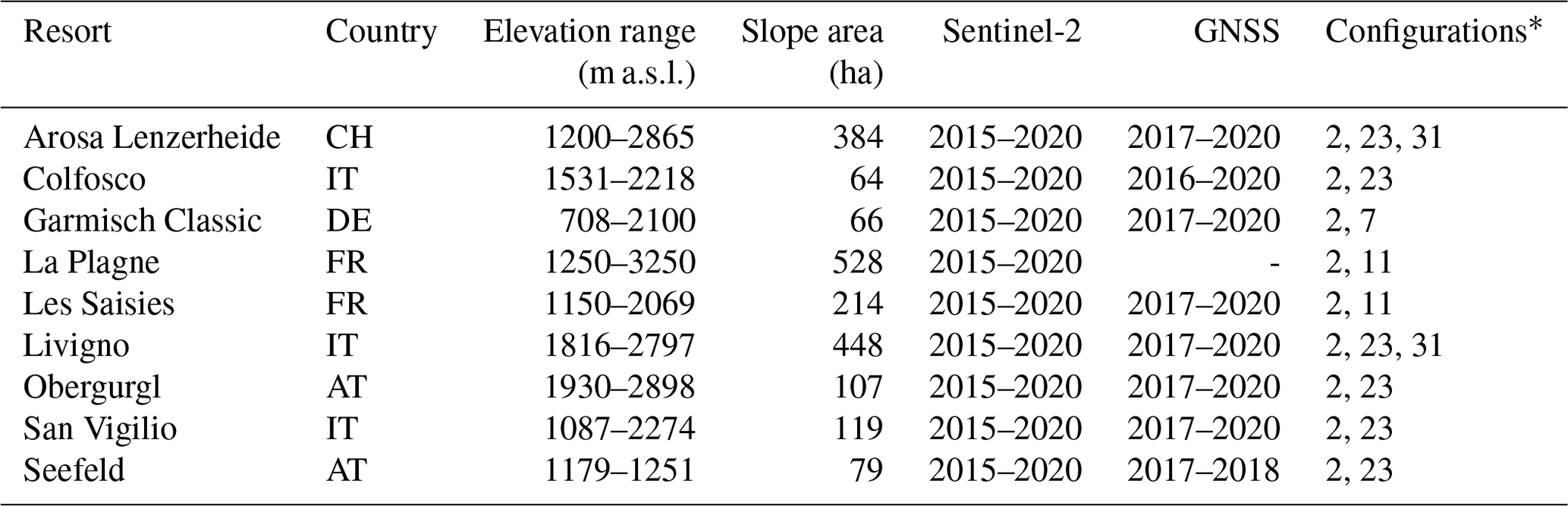
Table 1 Overview of the nine PROSNOW ski resorts, the period of available Sentinel-2 and measured GNSS snow depth data, and the used snow management configurations for the simulations based on the paper by Hanzer et al. (2020).

^* Hanzer et al. (2020)

The objective of this paper is to evaluate the accuracy of the piste snow management module refined and implemented in the framework of the H2020 PROSNOW project embedded within several snowpack models to simulate snow management in general and for each individual PROSNOW ski resort in high spatial resolution. In a first step, the results of the snowpack simulations were compared both with remotely sensed satellite snow cover maps and with snow depth measurements spatially distributed along the ski slopes acquired with specific GNSS systems. The impact of elevation, slope, and aspect as well as temporal aspects within a season or amongst different years was evaluated. In the second step, the simulation domain was spatially discretized into defined ski resort reference units (SRUs) (Hanzer et al., 2020) to reduce computational effort but still be able to achieve meaningful results. In this case, each ski resort was divided into a number of elevation bands with widths ranging from 50 to 400 m.

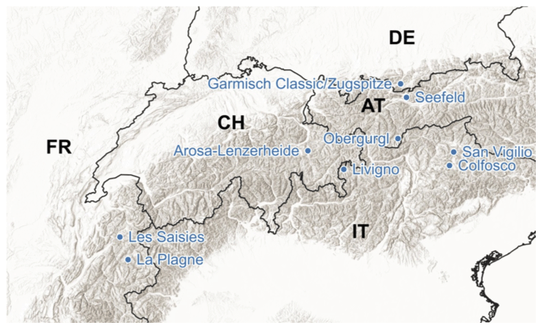
Figure 1 Locations of the PROSNOW ski resorts.

2 Study sites, models, and data

2.1 Ski resorts

Within the PROSNOW project we focused on the following nine ski resorts, which are also all part of this study: Seefeld (cross-country part) and Obergurgl in Austria; La Plagne and Les Saisies in France; Garmisch Classic in Germany; Colfosco, San Vigilio, and Livigno in Italy; and Arosa Lenzerheide in Switzerland. This selection of ski resorts represents a large diversity of geographical, climatical, and snow-making practices and equipment. Figure 1 and Table 1 show the locations and key characteristics of the resorts.

2.2 Snowpack models

Snowpack simulations are performed with AMUNDSEN for the Austrian and the Italian resorts (Colfosco, Obergurgl, San Vigilio, and Seefeld), with Crocus for the French resorts (La Plagne and Les Saisies) and with SNOWPACK–Alpine3D for the remaining resorts in Switzerland, Germany, and Italy (Arosa Lenzerheide, Garmisch Classic, and Livigno). We used for each ski resort different settings for the parameters concerning wet-bulb temperature, snow depth threshold, timing, and density of grooming. A detailed description of the functionality and parameters of the snow-making and grooming modules, which are used in all of the snowpack models, is shown in the study by Hanzer et al. (2020) and the applied configuration for each ski resort in Table 1. The three snowpack models, AMUNDSEN, Crocus, and SNOWPACK–Alpine3D, are well established and have been widely applied in numerous studies throughout the past decades (Essery et al., 2020; Krinner et al., 2018).

All three models require spatial input data for the snow management simulations consisting of a digital elevation model (DEM) covering the study sites, the locations of the ski slopes, and the locations and types of the snow guns (snow lances or snow fans – corresponding to different production rates for given ambient conditions as defined in Table 5 in Hanzer et al., 2020). The snow management configurations employed for each ski resort are shown in Table 1 and are selected to be representative of the snow management configuration of each ski resort based on individual discussions with the ski resort managers. In general, the basis for snow production relies on resource saving assumptions, the features of the locally installed snow-making system, and the opening and closing of each ski resort. The configurations were selected for each ski resort as follows and are described in more detail in Hanzer et al. (2020):

• configuration 2: no snow production; simulations based on a natural snow-only configuration, however with grooming activity

• configuration 7: snow production with a minimum required snow water equivalent (SWE) of 150 kg m⁻² using snow fans and a wet-bulb temperature of maximum −4 ^∘C

• configuration 11: snow production with a minimum required SWE of 150 kg m⁻² using snow lances and a wet-bulb temperature of maximum −4 ^∘C

• configuration 23: snow production with a minimum required SWE of 250 kg m⁻² using snow fans and a wet-bulb temperature of maximum −4 ^∘C

• configuration 31: snow production with a minimum required SWE of 250 kg m⁻² using snow lances and a wet-bulb temperature of maximum −6 ^∘C

Meteorological forcing data for the simulations are based on measurements from automatic weather stations close to or within the study sites and from the SAFRAN analysis for Crocus model runs (Vernay et al., 2019), consisting of at least hourly measurements of air temperature, precipitation, relative humidity, wind speed, and radiation. The generated output data are rasterized snow depth files with a resolution of 10 m.

The models are equipped with a machine-made snow production and grooming module, which can be used for the operational applications. A set of core parameters can be used for very detailed simulations of snow management practices in single ski resorts. They take into account snow demand, the meteorological conditions including information on wet-bulb temperature and wind speed, and the ski resort infrastructure in terms of the amount of snow that can be produced in a given time step at a certain location within the resort. For the simulations it is assumed that for a given snow gun, all of the produced snow is distributed immediately and evenly over a predefined slope section. Additionally, the grooming module allows the distinct properties of groomed snow on ski slopes to be accounted for depending on the amount of snow present and a defined grooming schedule. It assumes that grooming has no effect on the distribution of snow, e.g., shifting of snow from one place to another, but rather only compacts it (Hanzer et al., 2020).

2.3 Ski resort reference unit – SRU

Real-time simulations with a very fine spatial resolution (i.e., 10 m) require a very high computational demand, and such fine spatial resolutions are also often not necessary for the overall day-to-day resort management. Spatial clustering of slopes and slope sections is often sufficient for the snow managers working in an operational mode. Therefore, we additionally discretized each ski resort in ski resort reference units (SRUs). In a post-processing step, we aggregated the initial 10 m pixel size to larger areas. We defined different SRU sizes of the individual pistes by slicing them into the following elevation step ranges: 50, 100, 200, 300, and 400 m. Local snow management plays a major role in the SRU sizes as explained in more detail in Appendix A1. This aggregation results in different numbers of SRUs for each considered elevation range. Figure 2 exemplarily shows a map for the western part of Arosa Lenzerheide with the resulting elevation classes for the different SRU sizes. In addition, we evaluated the sensitivity of SRU size to the final accuracy. More details about the SRU definition can be found in Appendix A1 and Table A2.

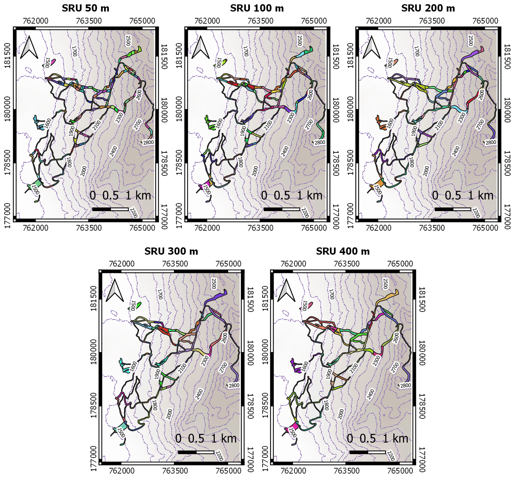
Figure 2 An example of a ski resort discretization into different SRU elevation bands: 50, 100, 200, 300, and 400 m. The figure shows the western part of Arosa Lenzerheide. The different colors represent the different SRU areas.

2.4 Sentinel-2 data

The model results for all ski resorts were compared with remote sensing images; for this study, Sentinel-2 (S2) data were used. The processing of the S2 snow-covered maps was done in three main stages: (i) calibration to top-of-the-atmosphere (ToA) reflectances; (ii) re-projection, resampling, and co-registration with the model grid with a final resolution of 10 m; and (iii) classification with a support vector machine (SVM) classifier trained with an active learning procedure (Tuia et al., 2016). In particular, the classification was devoted to both (i) detecting the clouds and (ii) detecting the snow presence. This was done by exploiting the most representative features for each of the two classification problems. In detail, we used all the spectral bands, the normalized difference snow index (NDSI), and the normalized difference vegetation index (NDVI) for the cloud classification. NDVI was calculated as the normalized difference between near-infrared (NIR) and red bands, whereas NDSI was calculated between green and shortwave infrared (SWIR) bands. Regarding the snow detection, we used the spectral bands, NDSI, NDVI, and the illumination angle calculated from the solar zenith and the solar azimuth angle (Riaño et al., 2003).

Since the S2 snow maps are compared to the snow simulations, particular attention was devoted to obtain accurate results. For this purpose, three main steps were performed to address the main problems related to snow classification from optical images, which are the detection of (i) particular cloud conditions; (ii) the mixed snow pixels, i.e., pixels in which classes other than the snow contribute to the observed spectral response; and (iii) the snow under the canopy of the forests.

First, we performed a visual analysis of all the S2 images for excluding the scenes presenting complex cloud conditions. In particular, semitransparent clouds, which are thin, high-altitude clouds composed of ice crystals, were detected from the S2 band acquired at 1.375 µm. Interestingly, semitransparent clouds might not be visible in other spectral bands, but they alter the spectral signatures, leading to unreliable results.

The SVM classifier was trained in a way that a pixel with at least 50 % snow coverage is classified as snow. This means that, for example, during the snow-making production at the beginning of the season, a pixel in which significant snow production is ongoing is classified as snow even though not all of the pixel area is covered with snow. Additionally, we identify the shadowed areas from where the multispectral sensor on board S2 is not able to record sufficient energy for distinguishing between snow and snow-free areas. This happens when the sun is low at the horizon approximately from mid-November to mid-February, and the terrain is extremely steep. In all the other shadow cases, the SVM classifier was trained to detect the snow presence. Hence, the output of the procedure was a classified map with four classes, i.e., snow, snow-free, shadows and clouds.

Since the detection of snow under forest canopy is a challenging research topic from both the remote sensing and modeling point of view, we conservatively masked out forested areas for all the ski resorts based on the land cover classification provided by OpenStreetMap (OSM) (resolution of 30 m) (Schultz et al., 2017), rasterized to a resolution of 10 m and manually refined for all ski resorts in such a way that the ski slopes that were passing through forest but were visible at the resolution of S2 were considered for the evaluation. The masked layers include coniferous, deciduous, and mixed forests and in some particular cases also scrubs and heath. After this screening all the snow maps were considered reliable, and the scenes with a percentage lower than 50 % cloud were retained as sufficient information for the cross-comparison.

A detailed overview of the number of available S2 scenes for each year and ski resort is presented in Table A1 and Figs. A1 and A2 in the Appendix. The number of S2 scenes which were available for each ski resort within the winter periods of 2015 to 2020 is in general high and ranges between 62 and 190 per ski resort. The differences in numbers of available scenes were mainly affected by cloud coverage and the atmospheric condition to perform accurate classification.

2.5 GNSS snow depth data

More and more ski resorts are relying on spatially distributed snow depth measurements performed with modern Global Navigation Satellite System (GNSS) technology for an efficient management of their slopes. This technique relies on differential GNSS signals, comparing the snow-free (i.e., zero snow depth) reference signal with those obtained during the snow season to obtain snow depth. The sensors are installed on top of the groomers, and thereafter snow depth can be tracked as a positive side effect whilst grooming the pistes. This technology ensures a snow depth measurement accuracy down to the centimeter level and at a spatial resolution of 1 m, which also allows the tracking of snow redistribution with the groomers.

For our study, rasterized data were provided by the companies SNOWsat and Leica Geosystems AG and were resampled to a resolution of 10 m using the average value in order to be directly comparable with the model outputs. The GNSS snow depth data were available for all ski resorts except La Plagne. We considered for the analysis the measurements spanning from 1 December to 31 March with a daily temporal resolution when GNSS data were available. The data have been preprocessed to eliminate outliers and to check their consistency. Table 1 shows the available seasons of GNSS snow depth measurements for all ski resorts.

3 Evaluation

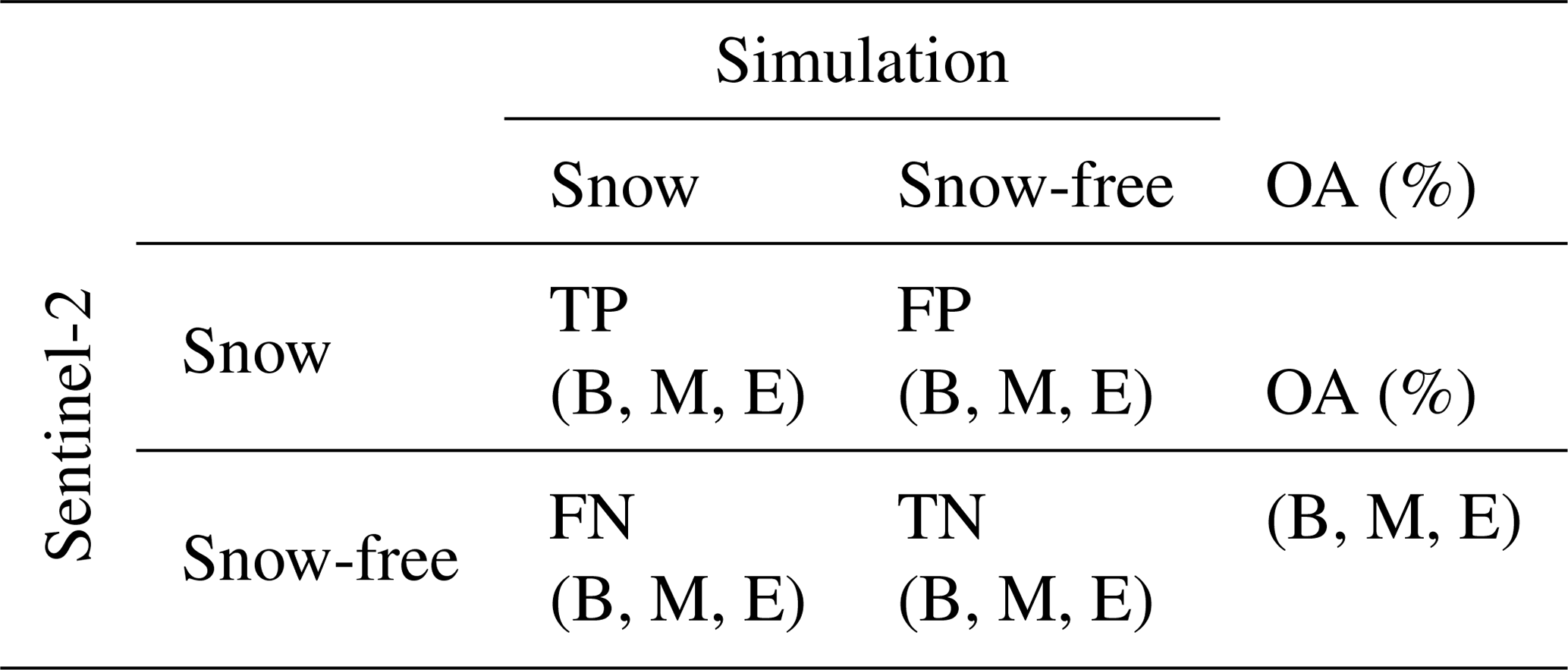
In this section, we describe how we evaluate the snowpack simulations carried out for the PROSNOW ski resorts. This includes (i) the evaluation of snow-covered area and (ii) the evaluation of simulated snow depth. In detail, the simulated snow depth was compared with the GNSS-derived measurements over a number of ski slopes, whereas the snow-covered area is evaluated by comparing the model snow-covered area with the S2 snow maps. The metrics used for assessing the agreement between the simulations and S2 snow maps are the confusion matrix and the snow persistence index defined below.

The evaluation analysis for both snow depth and snow-covered area was conducted by stratifying the data according to temporal and topographical constraints. Moreover, a differentiation was made between natural snow, i.e., snow outside the pistes, and managed snow, i.e., snow inside the pistes. In the following subsections more details on how the evaluation metrics were calculated are presented.

3.1 Snow coverage – snow persistence (SP) and confusion matrix (CM)

The latitude, longitude, and elevation of a ski resort have a big impact on the timing of snow accumulation and melt. Therefore, comparing snow patterns between regions is challenging despite the widespread application of remotely sensed methods for snow research. The snow persistence (SP) is a snow metric that can be used to map snow zones globally (Macander et al., 2015; Wayand et al., 2018; Vionnet et al., 2020). It is calculated in this work as the number of snow-covered days divided by the number of valid Sentinel-2 observations for the whole period (5 years). The number of total observations can vary for each pixel since cloudy or masked pixels are not considered for the computation. Hence, the same valid dates are considered for the model. This approach has been used in a wide range of climates (Richer et al., 2013; Moore et al., 2015; Saavedra et al., 2017) to identify transitions between rainfall and snowmelt peak streamflow source regimes (Kampf and Lefsky, 2016) and for predicting water yield (Saavedra et al., 2017; Hammond et al., 2018).

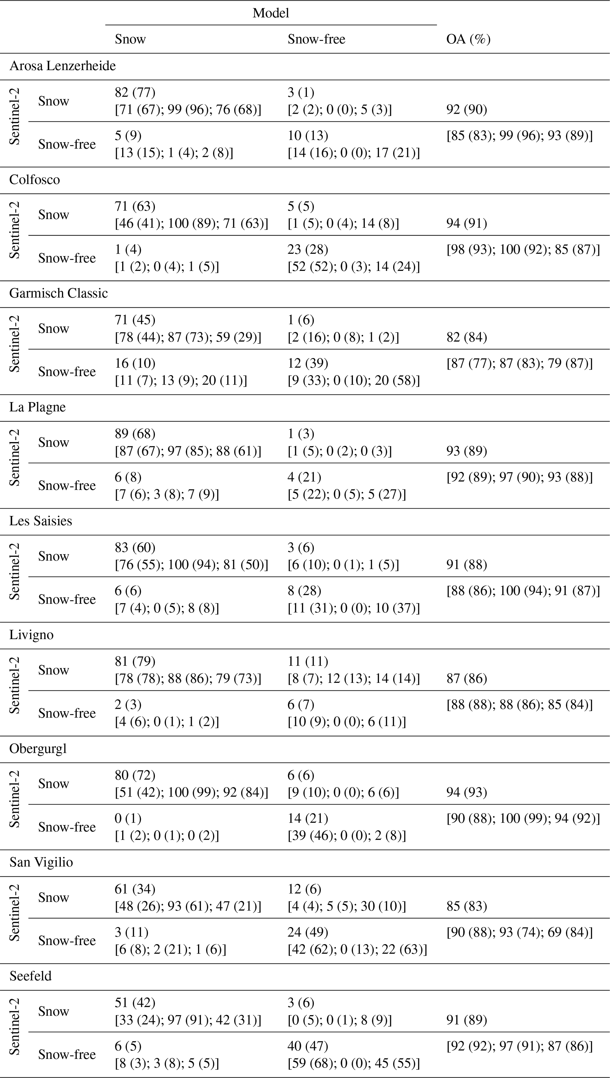
Table 2 Example of the confusion matrix used in the “Results” section. The analysis was split into three periods: beginning (B: October–November–December), middle (M: January–February), and end (E: March–April–May) of the season. TP: true positive; FP: false positive; FN: false negative; TN: true negative; OA: overall agreement.

Two SP indices were extracted considering both S2 snow maps and model simulation. They were calculated pixel-wise as the ratio between the number of snow-covered days derived by S2 or from the model, divided by the total number of S2 observations (snow or snow-free). The values of SP were always between 0, i.e., always snow-free dates, and 1, i.e., always snow-covered dates. If an S2 snow map pixel is classified as a cloud the corresponding snow model output is masked out, preserving the one-to-one correspondence between the two SP indices.

In addition to the SP index, for each ski resort a confusion matrix was computed to assess the quality of the S2 and snowpack simulations. We refer to the confusion matrix as modeled vs. observed variables. The confusion matrix has the form indicated in Table 2 (TP: true positive, i.e., both model and S2 labeled as snow; FP: false positive, i.e., model labeled as snow, S2 as snow-free; FN: false negative, i.e., model labeled as snow-free, S2 as snow; and TN: true negative, i.e., both model and S2 labeled as snow-free). Therefore, TP and TN indicate that model and S2 data match with each other, whereas FP and FN indicate that they do not match.

We distinguish between natural snow and snow on the slopes. Furthermore, the analysis was split into three periods: beginning (B: October–November–December), middle (M: January–February), and end (E: March–April–May) of the season. A pixel can be either true (snow in S2 data and model, no snow in S2 data and model) or false (snow in S2 data and no snow in model, snow in model and no snow in S2 data). With the accumulation of all pixels assigned to be true, an overall agreement OA (%) was calculated for each period and catchment:

$$\begin{array}{}\text{(1)}& \mathrm{OA}={\displaystyle \frac{\mathrm{TP}+\mathrm{TN}}{\mathrm{TP}+\mathrm{FP}+\mathrm{TN}+\mathrm{FN}}},\end{array}$$

which describes how often the agreement between S2 and the simulations was correct.

3.2 Snow depth – root mean square deviation (RMSD) and mean deviation (MD)

The metrics used for this assessment are the mean deviation (MD) and the root mean square deviation (RMSD) over time for each ski resort. Regarding the snow-covered area evaluation, the binarization of the simulated snow depth to the snow-covered map was done by imposing a threshold of 0.05 m; i.e., every value above this threshold was identified as snow, while in contrast all the values below 0.05 m were identified as snow-free. This threshold is in line with previous works (Notarnicola, 2020). In each defined SRU we analyzed the variations in terms of snow depth MD and RMSD. The MD was used to relate between the modeled and measured snow depth on the slopes among years for the period October to May. Measured snow depth data from all available years of observations (see Table 1) were used in order to analyze the quality of the simulated snow management configuration for each ski resort. This allowed better projection of the uncertainty in the simulated snow management configuration based upon the measured snow depth. RMSD and MD per one time point are defined as

$$\begin{array}{}\text{(2)}& \begin{array}{rl}& \mathrm{RMSD}=\sqrt{{\displaystyle \frac{\mathrm{1}}{N}}\sum _{i=\mathrm{1}}^N{\left({\text{SD}}_{\mathrm{m}}\left(i\right)-{\text{SD}}_{\mathrm{s}}\left(i\right)\right)}^{\mathrm{2}}}\\ & \mathrm{MD}={\displaystyle \frac{\mathrm{1}}{N}}\sum _{i=\mathrm{1}}^N\left({\text{SD}}_{\mathrm{m}}\left(i\right)-{\text{SD}}_{\mathrm{s}}\left(i\right)\right),\end{array}\end{array}$$

where N is the number of valid pixels for a given date, SD_m is the GNSS snow depth measured, and SD_s is the snow depth simulated by the model. Hence, the metrics were calculated based on pixels and only on those pixels where GNSS measurements were present; i.e., the number of considered pixels N can vary for each date. A negative MD value indicates an overestimation, and a positive MD value indicates an underestimation of the snow persistence of the PROSNOW models.

4 Results

In this section, the simulated results for all ski resorts were compared with the S2-measured snow cover and with the GNSS-measured snow depth data on the ski slopes. Model runs were performed for five winter seasons (2015–2020) from 1 October until the end of May. The simulations were carried out for all ski resorts using the default snow management configurations accounting for both fan guns and lance guns as well as different temperature thresholds and base-layer production targets, given in Table 1. The configurations were either assumed or provided by the person responsible for snow-making at each ski resort.

Table 3 Confusion matrix for all ski resorts referring to snow on the pistes. The values in the parentheses are referring to natural snow. The metrics in the square brackets also refer only to snow at the beginning, middle, and end of the season.

4.1 Snow coverage

The S2 algorithm produced accurate snow maps with an overall accuracy above 80 %, for both high-Alpine and lower-lying mountainous regions and different stages of the season like season start, mid-season, and end of season. A first approach to assess the skills of the models using S2 maps as a reference was a confusion matrix. Table 3 presents the results for each ski resort. Analyses were carried out for solely regarding snow on the pistes and additionally also for the complete ski resorts, including the off-piste areas. The overall accuracy for natural snow (off-piste) is around 80 %. Regarding the pistes, where we applied the snow management, we could further increase the overall accuracy up to 85 %. Based on this we can conclude that the integration of the snow management module in the snowpack models increases the performance within the ski resorts, which is also obvious in the early and late season, shown in the Appendix (Figs. A2 and A1). The snow distribution was well simulated at the beginning and end of the season, with an agreement of over 79 %. However, a larger mismatch was observed for San Vigilio with 69 % at the end of the season because of the overestimation caused mainly by the ablation process in the snow model. A higher agreement between the simulation and the S2 data was observed when regarding the pistes only. Compared to the analysis of the entire resort, including natural snow, the overall accuracy of pistes only was up to 8 % higher. Only one resort (Garmisch Classic) showed a slightly lower accuracy of 8 % on pistes as the majority of pistes are situated in forested areas, where it is difficult to capture the pistes via satellite images.

Figure 3 Snow persistence index difference between Sentinel-2 data and the model data (on the left) and SP indices for the simulation and Sentinel-2 (on the right) for each ski resort: (a) Arosa Lenzerheide, (b) Colfosco, (c) Garmisch Classic, (d) La Plagne, (e) Les Saisies, (f) Livigno, (g) Obergurgl, (h)  San Vigilio, and (i) Seefeld. The period 2015–2020 was considered, when valid Sentinel-2 data are available.

The snow coverage quality of the snowpack simulations using the snow management modules was further assessed using the S2 data and SP indices. The SP indices were calculated for the simulations and S2 data, and the relative differences are shown in Fig. 3. The green pixels indicated the applied forest mask to minimize the underestimation of snow detection by the S2 algorithm. Observed SP presented similar patterns for each ski resort, showing that snow persistence patterns were primarily controlled by the elevation. High elevation corresponds to high SP values, whereas low SP values were found near the tree line and at lower elevations. In addition, low SP values were also found near ridge lines, exposed to wind, and influenced by lateral snow redistribution and snow accumulation. These effects were not captured by the simulations. Further, the derived SP values were dependent upon the elevation and slope orientation, primarily due to the impact of solar radiation on simulated snow ablation. The biggest difference in the SP index between the S2 data and model was found in steep slopes, where the effect of snow gliding (e.g., avalanches) is stronger.

The overall accuracy was mainly impacted by the elevation and slope. An interesting analysis was represented by the trend of the overall accuracy over 100 m elevation classes, 5^∘ slope classes, and 45^∘ aspect classes (i.e., north, northeast, east, southeast, south, southwest, west, northwest). This analysis was carried out taking specifically only the snow on the pistes into account and is presented in Fig. 4 (left). The agreement of the simulations with the S2 data increased with increasing elevation by around 1 % per 100 m elevation class. The overall accuracy over 5^∘ slope classes is not affected by the slope steepness, and the orientation of the slope towards the sun showed no influence on the accuracy.

A closer look at the SP index showed an elevation dependency, but a clear slope or aspect dependency is hard to detect. A better accuracy is obtained at high altitudes due to the fact that the ratio of snow cover area is near 1. Figure 4 (middle) shows the difference between S2 and model SP index, similar to Fig. 4 (left). Positive values indicated an underestimation of the model with respect to S2. Above 2000 m, the MD SP index is close to zero, and the model results are consistent with the S2 data. However, below 2000 m the MD increases as most of the slopes are equipped with snow-making facilities and are affected by local snow management adjustments due to local snow and weather conditions.

Figure 4 Comparison for 100 m elevation bands, 5^∘ slope bands, and 45^∘ aspect bands for (left) overall accuracy (OA) between simulation and S2 data, (middle) mean deviation (MD) in snow persistence index between S2 data and simulation, and (right) mean deviation (MD) value between the simulated and GNSS-measured snow depth data. All metrics are computed for snow on the pistes only.

4.2 Snow depth

The simulated default snow management configurations reproduced the actual conditions well at all ski resorts. Figure 5 shows the RMSD and the MD between the modeled and GNSS-measured snow depth over time for each ski resort and each season. Especially at the beginning of the season, the RMSD values between the simulated and the GNSS-measured snow depth on the pistes were below 0.4 m on average. However, the RMSD values slightly increased during the season affected by daily adaption of the snow management configurations due to the actual weather conditions. The complexity of the snow management configuration increased during the season, leading to an increase in the RMSD values at the end of the season. In general, the temporal evolution of the RMSD values shows almost no large peaks. The large peak at Lenzerheide on 15 January 2019, occurred due to a heavy snowfall period, which led to an extraordinary avalanche situation. As a result, a large part of the ski area was closed, and many slopes were no longer groomed at this date. This led to the strong increase in the RMSD values in this season. In general, our models mainly overestimated the snow depth, and the fluctuations increased during the season. Regarding the degree of linear dependency of the simulated and measured data, the MD as shown in Fig. 5 reaches more than 0.5 m at some resorts, suggesting that more snow was produced compared to the model. For several resorts an increase in MD can be observed especially at the end of the seasons.

Figure 4 (right) represents the MD trends between the simulated and GNSS snow depth data for 100 m altitudinal classes, 5^∘ slope classes, and 45^∘ aspect classes. For this analysis, we considered RMSD values which refer to all the pixels corresponding to a fixed elevation class, degree slope, or degree aspect class, respectively, calculated over all the available days. Overall, the MD values vary between −0.6 and 0.6 m. No systematic relationship can be seen between the elevation and steepness of the pistes; the curves are highly specific for each resort. However, regarding the elevation discretization, the MD values increase on average with increasing elevation. An overall average MD trend on the 5^∘ slope classes is not found. Only for Arosa Lenzerheide, Garmisch Classic, and Les Saisies was a decrease in MD values for steeper slopes observed. The analysis of the 45^∘ slope aspect bands on the MD values shows that the accuracy decreases for slopes oriented mainly towards the southwest. This is primarily due to the impact of solar radiation on the snow ablation.

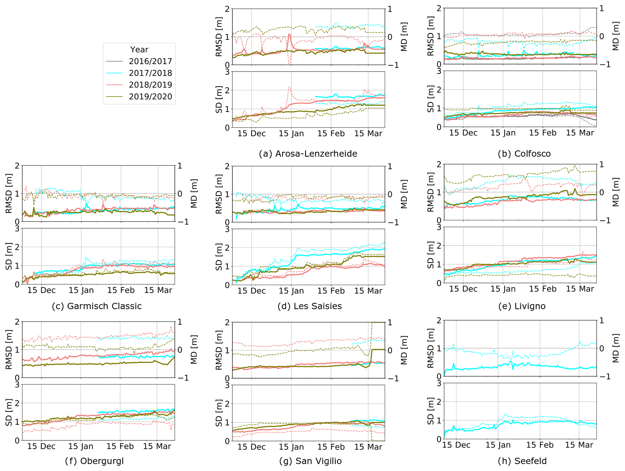
Figure 5 Root mean square deviation (RMSD) (upper subplots: solid line, left axis) and mean deviation (MD) (upper subplots: dashed line, right axis) averaged over space between GNSS-measured snow depth (SD) (lower subplots: solid line, left axis) and simulated SD (lower subplots: dashed line, right axis) over time for the ski resorts. Within the period 2016–2020 we considered all valid GNSS-measured snow depth data which were available.

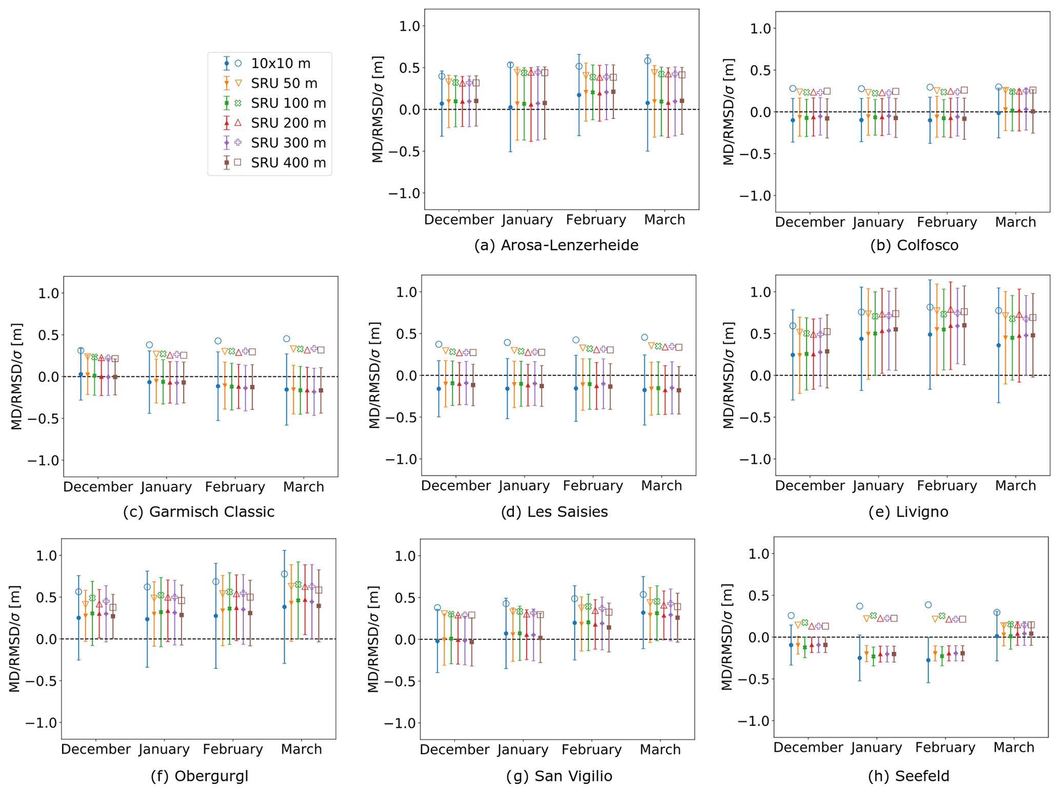
Figure 6 Overview of the root mean square deviation (RMSD; hollow symbols), mean deviation (MD; filled symbols), and standard deviation (σ; extent of error bars) between simulated and GNSS-measured snow depth considering all the time steps and displayed for each different SRU resolution for the entire ski resort. The presented data are analyzed for the 4 months December, January, February, and March, when GNSS data were available.

4.3 SRU discretization

Discretizing the ski resorts in coarser clusters tends to mask the variability in the error in terms of RMSD due to averaging effects between the simulations and GNSS-measured snow depth between 8 % and 45 % independent of the season and cluster size (see Table A2). Therefore, it was not possible to find an overall optimal SRU size regarding the RMSD values. We also computed the MD of the errors calculated as the difference between the measured snow depth and the modeled snow depth, shown in Fig. 6. The original pixel snow depth is kept for the 10 m resolution, while a mean snow depth for each SRU is calculated for the different SRU altitudinal band classes. For the computation of the SRU snow depth, only those pixels with valid GNSS measurements were considered and taken into account (between 0 and 3.5 m). The MD and the standard deviation of the error are then calculated by considering all the available measurements over time and space. We propose here a differentiation for the 4 months December, January, February, and March in Fig. 6. Interestingly, the mean and the deviation of the MD values widely differ for single resorts.

In addition, we tested the spatial variability within the pistes. For a visualization example presented in Fig. 7, we chose a long piste ranging between 700 and 1700 m a.s.l. within the Garmisch Classic ski resort for a date with maximal piste coverage. Figure 7 reports the simulated snow depth and the GNSS measurements as well as the pixel-wise difference for the original resolution at 10 m (on the left). The same variables averaged over a possible SRU discretization, in this specific case considering 100 m elevation bands, are also reported in the same figure on the right. Regarding the fine resolution of 10 m, it is obvious that the GNSS snow depth data are much more variable in general and are especially available in the upper part of this piste due to the more highly localized snow management than the simulations with the default configuration can provide and due to small-scale topographic differences in some regions of the pistes. A good agreement was found especially in the lower and middle parts of this example slope, with slight under- and overestimations of the simulated snow height. The picture would look similar for all other pistes and resorts (not shown).

5 Discussion

This study presents a new high-resolution evaluation of snowpack simulations including snow management modules for mountain ski resorts to assess the quality of the simulations. The simulated results showed a high overall accuracy of more than 80 % compared to the Sentinel-2 data and a root mean square error in the GNSS-measured snow depth of below 0.6 m. The simulated results for all ski resorts are plausible and robust on the ski slope scale.

5.1 Snow coverage

For every ski resort, a large number of S2 images classified with high accuracy were available to assess the quality of the simulations in terms of snow coverage. More than 62 S2 images at each ski resort and even more than 150 for two resorts were analyzed. The specific machine learning algorithm to derive information with low uncertainty about the presence or absence of snow from the Copernicus Sentinel-2 images allows the generation of snow maps across the Alps with relatively low manual effort. Additionally, the very detailed forest mask applied to the evaluation allowed us to simultaneously (i) avoid situations for which the information provided by S2 is insufficient to produce accurate results and (ii) be able to extract information about the snow cover for the pistes crossing dense forests, as is often the case for Garmisch. This allowed us to minimize the pixel loss due to canopy shading. The highest pixel losses with respect to the total piste area were in Arosa Lenzerheide (5.7 %) and Seefeld (5.5 %), followed by Obergurgl (2.4 %), Livigno (0.2 %), and Colfosco (0.2 %). For the other ski resorts it was zero.

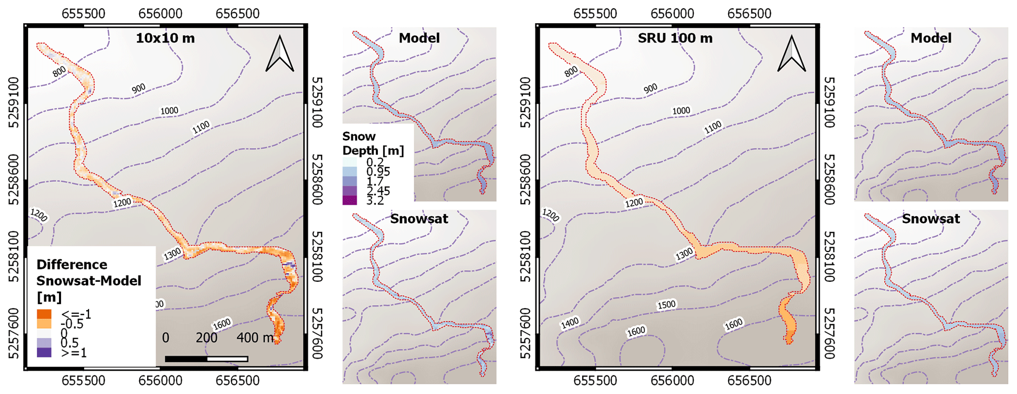
Figure 7 Example of spatial variability within a piste in Garmisch Classic (22 January 2018). On the left, RMSD represented as pixel-wise difference between measured and modeled snow depth for a 10 m pixel resolution. The smaller figures represent the original modeled and measured snow depth. On the right, RMSD represented as averaged difference between measured and modeled snow depth for a 100 m band SRU resolution. The nature of the large measured snow depth by GNSS at around 1400 m elevation is due to a dip in the ground surface, which was filled with snow to level the piste. This led to a higher GNSS-measured snow depth compared to the simulations.

The underestimation of the overall accuracy at the beginning and the end of the seasons was due to the fact that sometimes the exact snowline in the S2 data was hard to detect. Some snow lines were obscured by shadows, and they often did not appear as continuous lines, which may slightly bias our regional estimates, especially in areas which span different land uses. Also white rock types or illuminated wet rocks can lead to brighter pixels in the S2 data and to an underestimation of the overall accuracy. Because the spectral signal of these pixels is similar to that of snow, the algorithm detects an ice–snow boundary and classifies these pixels as part of the snow lines. Since these patches were situated in ski resorts in rocky areas, these misclassified pixels introduced negative biases in the overall accuracy estimates, and they were filtered out manually.

By inter-comparing the model simulations and the S2 images we encountered some recurrent errors. As described in the previous section, on average the accuracy of the simulations is high, and the snow coverage simulated by the PROSNOW models is consistent with observations. However, wrong discretization and/or missing meteorological input and lack of snow managing or land use information were the main sources of errors. In particular, (1) ephemeral snow (i.e., snow that lasts a few days either at the beginning or at the end of the season) is difficult for the models to simulate correctly; (2) rain–snow transition (e.g., ensuing rapid snowmelt inside the catchment) is difficult to simulate accurately; (3) due to unknown snow-making strategies, which are then not incorporated into the PROSNOW models, snow-making at the beginning of the season and delayed and anticipated snow melting at the end of the seasons are not correctly modeled over managed slopes; and (4) the heterogeneous landscape at 10 m resolution plays a role in the snow accumulation and melting dynamics (e.g., towns, lakes, and roads are visible and change the snow distribution). This information is generally not addressed by the PROSNOW models. These are just confirmations of the expected limitations of the state-of-the-art snow cover models. However, for the first time a systematic and extensive evaluation at high model resolution was performed. The details of the analysis with all the different recurrent errors encountered for each ski resort are shown in Table A3 and can be used for future studies. Note that the simulations presented here do not benefit from snow depth measurements and water consumption of snow-making, which are used, upon availability of the relevant data, for real-time applications of the models for operating the PROSNOW service provision, thereby limiting the impacts of some of the caveats identified above.

5.2 Snow depth

The GNSS data can only be used as ground observations with some restrictions. There are several problems which might affect the quality of the GNSS data: (i) the digital elevation model (DEM) profile of all ski resorts is prone to change every year due to earthwork and adaption of the slopes and is always considered correctly in the extraction of the snow depth, and (ii) the inclination of the groomer has a large impact on the GNSS-measured snow depth. For example if the calculated snow depth is 0.5 m, the effect of 30 % inclination would be 6 cm, which means that the calculated snow depth would be 12 % higher than in reality. Furthermore, the work of the groomers is not only to measure the local snow depth but also to fill sinks, compensate humps, or level out the snow production or redistribution by the skiers. This might lead to very small-scale variances in the GNSS-derived snow depth for pistes both with and without technical snow production, whereas the model shows less pronounced variability. Therefore, especially the small-scale deviations between the simulated and GNSS-measured snow depth are not well applicable to reflect the model accuracy. The comparison rather shows the degree to which the default snow management configuration was applicable for the individual ski resorts. As each ski resort spontaneously adapts its snow management production due to changing weather and snow height conditions, it is not possible to consider the spontaneous snow management adjustments during the season in the simulations. It does not make a big difference between pistes with and without technical snow production even though the models do not explicitly simulate the snow redistribution. However, the RMSD between the modeled snow depth and GNSS measurements over time for the ski resorts is in the uncertainty range of the simulated configuration. Hanzer et al. (2020) analyzed 10 different snow management configurations, and an uncertainty range in snow depth of 20–50 cm was observed. This shows that the default snow management configuration leads, in general, to satisfactory simulation results for the individual ski resorts.

Some recurrent errors are encountered by inter-comparing the model simulations and the GNSS-measured snow depth. The quality of the simulations is high, and they showed plausible and robust results on the ski slope scale. However, there are still sources of errors: (1) extreme snowfall situations, (2) snow redistribution by the groomers, (3) rapid ablation (e.g., south-, southwest-exposed pistes) due to high solar radiation, (4) levering of the pistes to reduce the accident risk of the skiers, (5) snow redistribution by the skiers, and (6) systematic errors due to the wrong snow-making strategy. These errors are already known, but it is too complex and not straightforward to consider this in the simulations in the current state. In detail, slightly different recurrent errors are encountered for each ski resort by inter-comparing the model simulations with GNSS-measured snow depth, which is shown in Table A3.

5.3 SRU discretization

Scale and data aggregation has important effects on the simulations and interpretation of snow depth data, which is also true for snow on pistes. Studies in different research fields clearly demonstrate that spatial variability and statistics are dependent on scale (Marceau, 1999; Wu, 1999; Wu et al., 2000; Perveen and James, 2010). Our evaluation showed that these scale dependencies in spatial variability and statistics appear complex with nonlinear increases with increasing grid-cell size. However a simple relationship between variability and scale emerges upon closer inspection: aggregating the 10 m simulated pixels to different SRU sizes led to a decrease in the error compared to the GNSS measurements due to averaging effects of the high spatial variability in the GNSS snow depth data. The RMSD values decreased between 8 % to 45 % regarding the SRU size using an altitudinal band of 50 m; however this effect diminished by further coarsening.

Nevertheless, the identification of guiding principles for researchers to combine data and models at different spatial and temporal scales and to extrapolate information between scales still remains a challenge. By going from fine to coarse scales, aggregation and generalization set in. The rate of information loss is influenced by small-scale spatial snow production and grooming patterns. Heterogeneous snow production for instance leads to more information loss than aggregations at coarser scales. The small-scale spatial effects of moving snow by the groomers or skiers, for instance, disappears slowly with decreasing resolution, and those that are dispersed are lost rapidly. This leads to an under- or overestimation of the simulated snow height. Therefore, a methodology needs to be developed to find out how much the loss of information takes place. Multiscale analysis was necessary to show that variability for different aggregation types of the snow height is inherently different and that for each SRU this can be different, as shown in Fig. 4.

However, we demonstrated a consistent evaluation procedure for all the PROSNOW ski resorts that can be useful for snowpack modelers and ski resort managers. An understanding of the nature of scaling effects is needed when spatial or temporal scale is an independent variable. In landscapes with homogeneous snow depths, where snow measurements can be summed directly, such scale problems may not occur. However, in snow-distributed landscapes like at ski resorts, snow measurements obtained at fine scales often cannot be summed directly to produce regional estimates. Therefore, reasonable measures are not always given by weighted averages because heterogeneity in snow production and distribution may influence scaling processes in nonlinear ways. In such cases, increasing the level of spatial heterogeneity may also increase the difficulty of extrapolating information across scales (Perveen and James, 2010).

5.4 Remote sensing and GNSS snow depth

The use of remote sensing and GNSS data allows an evaluation procedure to be defined for the snowpack models and helps to improve the resource management of the ski resorts. The GNSS data provide means to collect accurate snow depth points in the field for precise correction of the simulated snow depths. Further, using snow depth measurements over an entire season together with snowpack simulations is a powerful tool in the long term. It allows the estimation of the minimum snow depth required at various slope sections. This ensures that slopes are optimally prepared and groomed right up to the end of the season. The spatial remote sensing images are needed to improve the simulated snow-covered area, especially at the beginning or end of the season or for lower-situated ski resorts, where natural snow precipitation is low. Further, it allows the correction of the simulated ablation process at the end of the season and the snow produced at the beginning of the season. However, further studies to determine whether the models can simulate snow depth with sufficient accuracy to enable the resort mangers to maintain the optimum and minimum viable snow depth in a more efficient way are needed and will be attempted in the future (Köberl et al., 2021).

The combination of both techniques allows the evaluation and initialization of the simulations: imagery can be used for primary digitization of the snow cover where GNSS can be used for in situ observation of the snow height for the simulations. A detailed analysis of the differences between the two methods will allow us to make better decisions about when and how much snow is distributed by both groomers and skiers. Further, the effect of snow melting and snow redistribution by wind on the slopes can be extracted. This allows us to improve the models. However, this is not easy to extract and was not within the scope of this paper but should be considered for further studies.

6 Conclusions and outlook

The initiative for this study emerged within the H2020 PROSNOW project to evaluate the snow simulations over the nine PROSNOW ski resorts by comparing model outputs with local and remotely sensed measurements in terms of snow coverage, persistence, and snow depth. The three snowpack models AMUNDSEN, Crocus, and SNOWPACK–Alpine3D include all piste management modules and were evaluated using both ground-based data (GNSS-measured snow depth) and spaceborne Copernicus Sentinel-2-derived snow maps. We evaluated five winter seasons (2015–2020) from 1 October until the end of May and performed this evaluation in a stratified manner in order to assess the performance of the snow simulations under different conditions. Particular attention has been devoted to characterizing the spatial performance of the snowpack models with integrated snow management modules. Our presented results show high accuracy of the simulations, representing the “reality” well.

An inter-comparison of the three snowpack models applied to the same resort would be a logical next step from the model development perspective. Differences in the simulated results of the three models for a given ski resort would be mainly due to the different implementations of the snow management configurations into each model and due to the different snowpack energy and mass balance approaches. Such effects should have to be disentangled and discussed accordingly to have a reasonable comparison. However, this is not straightforward and is out of the scope of this paper but should be considered for the future. Nevertheless, this work showed that all three snowpack models applied for piste management reproduced plausible and robust results on the ski slope scale, and the overall accuracy of the results is mainly dependent on the degree to which the real-world snow management practices are integrated. Additionally, a detailed analysis to show the accuracy of the GNSS system installed on groomers to measure the snow depth is needed to validate the system. Moreover, integrating a snow redistribution model and an avalanche dynamics model into this system would help to point out where the biggest differences due to snow gliding or avalanches are between the Sentinel-2 data and the simulations. Further studies on the topographic complexity of the snow-free terrain and the rather smooth piste surface are needed to, for example, implement an index of surface smoothing compared to the bare ground. Future studies investigating how skiers redistribute snow under certain meteorological conditions in combination with topographic conditions (e.g., aspect, slope angle) would also help to overcome further potential errors.

Appendix A

A1 Further information on ski resort reference unit – SRU

In our approach, the spatial representations of ski areas and of the interpolated meteorological fields as well as the simulated snowpack information differ in their spatial representation: the geometry type used for the ski slope is a vector-based polygon, whereas the input and output of the snowpack models are based on a discrete approach, using regular grids of points. The challenge for PROSNOW was to define an intermediary spatial object. This should be consistent with representations balanced between the heterogeneity of meteorological conditions within ski slopes, the accuracy of snowpack models, and the computation resources and data volume required for a daily update. Also it should take into account the localization of the snowmaking facilities. The SRU, standing for ski resort reference unit, aims at fulfilling all of these requirements. It can be end-user-defined, including specific needs of the ski resort, but it can also be processed automatically by chaining several operations. We stored the vectorial geographic information system (GIS) and attribute data of all nine ski resorts in a PostgreSQL 10.7 database management system (DBMS), and the crossing operations between rasters and vectors were performed with Python 2.7 with the packages GDAL/OGR along with NumPy. For automatic processing of the SRUs we considered the following steps:

1. The association of each snow gun with a single ski slope is based on the spatial relation of the nearest neighbor to the ski slope.

2. The slope area covered by snowmaking is calculated by determination of the upper- and lower-altitude bounds for each snow gun. Considering that the mean surface covered by a single snow gun is approximately $\mathrm{1}/\mathrm{3}$ ha, we applied a procedural language (PL)/PostgreSQL function to calculate the intersection between a slope and incremental 5 m buffer around the snow gun point until it reached at least 3000 m². This buffer was then crossed with the combined ASTER–SRTM DEM v1.1 made available by the European Copernicus organization, and we kept the buffer's altitude bounds, which were then aggregated at the slope level to cover a continuous surface.

3. Once the snow type attribute (“grooming only” or “with snowmaking”) is defined for every slope, the according areas were then divided into smaller parts based on the elevation resolution. The initial DEM topography was reclassified with respect to the targeted SRU resolution. A value in the according numeric series was assigned to a pixel whose value is in the range of the target value of approximately half the resolution (i.e., for 50 m resolution, the value 300 will be assigned for all DEM pixels whose value is more than or equal to 275 m and less than 325 m and between 150 and 450 m for 300 m resolution). Contiguous pixels with the same values were merged and polygonized.

4. As small SRUs might occur by applying the abovementioned steps, e.g.,  at the beginning or ending of single pistes, we merged them in a post-processing step with other small adjacent piste fragments having the same snow type attribute. The final operation consisted of filling the missing snow type attributes by calculating the average area value for each polygon from the DEM and its derivatives (slopes and aspects) and matching the output from snow models (the snow type attributes of value, average altitudes (min and max altitude too), slopes, and aspects are also stored).

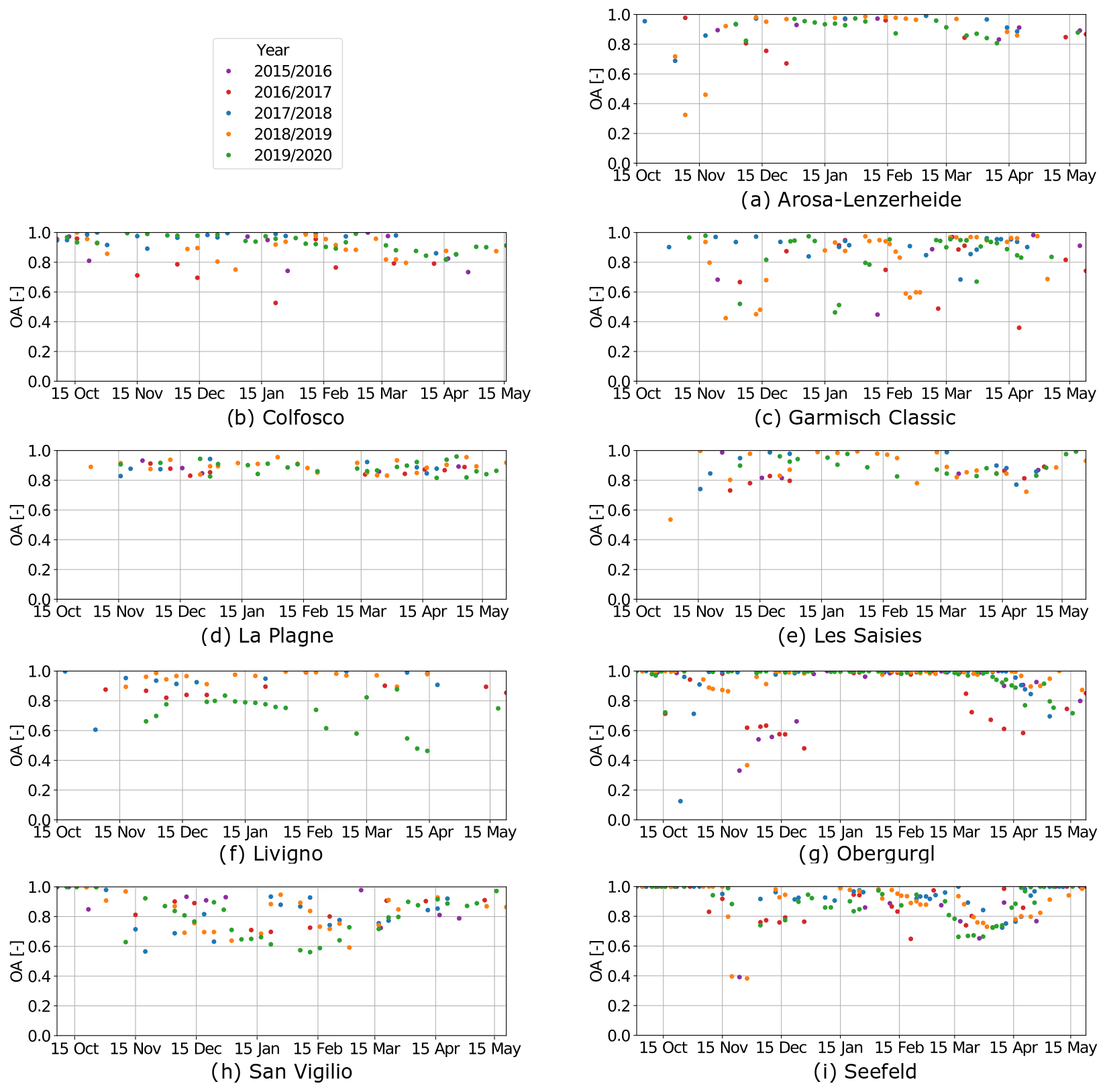
Figure A1 Overall agreement over time between simulation and S2 data for each ski resort for natural snow outside of the pistes. We considered images ranging from the winter season 2015/16 to the winter season 2019/20, except for Livigno, where simulations are not available for the first season 2015/16 due to gaps in the meteorological forcing data.

Figure A2 Overall accuracy trends over time between simulation and S2 data for each ski resort for machine-made snow on the pistes. We considered images ranging from the winter season 2015/16 to the winter season 2019/20, except for Livigno, where simulations are not available for the first season 2015/16 due to gaps in the meteorological forcing data.

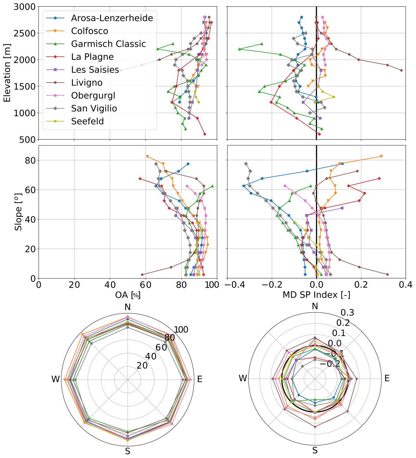
Figure A3 Comparison for 100 m elevation bands, 5^∘ slope bands, and 45^∘ aspect bands for (left) overall accuracy between simulation and S2 data and (right) mean deviation (MD) SP index between simulation and S2 data. All the metrics are computed for natural snow only.

Table A1 Total number of available Sentinel-2 data for each ski resort.

Table A2 Effect of discretization of the simulated results (10 m × 10 m) into different SRU elevation bands: 50, 100, 200, 300, and 400 m. The first line indicates the number of 10 m × 10 m raster points for each ski resort. The calculated root mean square error (RMSD), mean deviation (MD), and the standard deviation (SD) are between the GNSS-measured and simulated snow depth. GNSS data were not available for La Plagne.

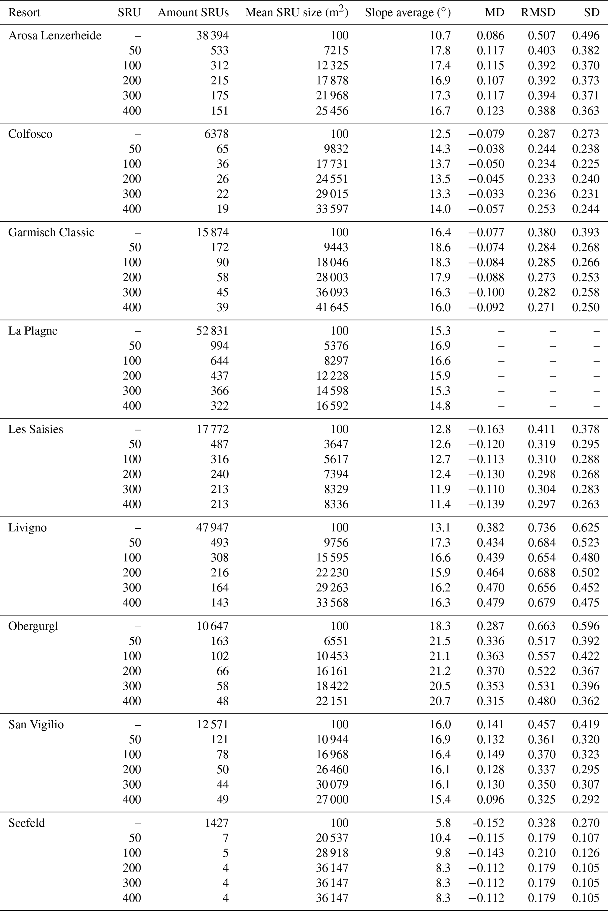
Table A3 Inter-comparing the model simulations with Sentinel-2 data and GNSS-measured snow depth for each ski resort.