the Creative Commons Attribution 4.0 License.
the Creative Commons Attribution 4.0 License.
 | 20 Aug 2021
Experimental and model-based investigation of the links between snow bidirectional reflectance and snow microstructure
Frederic Flin
Aleksey Malinka
Olivier Brissaud
Pascal Hagenmuller
Philippe Lapalus
Bernard Lesaffre
Anne Dufour
Neige Calonne
Sabine Rolland du Roscoat
Edward Ando
Snow stands out from materials at the Earth’s surface owing to its unique optical properties. Snow optical properties are sensitive to the snow microstructure, triggering potent climate feedbacks. The impacts of snow microstructure on its optical properties such as reflectance are, to date, only partially understood. However, precise modelling of snow reflectance, particularly bidirectional reflectance, are required in many problems, e.g. to correctly process satellite data over snow-covered areas. This study presents a dataset that combines bidirectional reflectance measurements over 500–2500 nm and the X-ray tomography of the snow microstructure for three snow samples of two different morphological types. The dataset is used to evaluate the stereological approach from Malinka (2014) that relates snow optical properties to the chord length distribution in the snow microstructure. The mean chord length and specific surface area (SSA) retrieved with this approach from the albedo spectrum and those measured by the X-ray tomography are in excellent agreement. The analysis of the 3D images has shown that the random chords of the ice phase obey the gamma distribution with the shape parameter m taking the value approximately equal to or a little greater than 2. For weak and intermediate absorption (high and medium albedo), the simulated bidirectional reflectances reproduce the measured ones accurately but tend to slightly overestimate the anisotropy of the radiation. For such absorptions the use of the exponential law for the ice chord length distribution instead of the one measured with the X-ray tomography does not affect the simulated reflectance. In contrast, under high absorption (albedo of a few percent), snow microstructure and especially facet orientation at the surface play a significant role in the reflectance, particularly at oblique viewing and incidence.
- Article
(9745 KB) - Full-text XML
- BibTeX
- EndNote


Snow optical properties are crucial to quantify the effect of snow cover on the Earth energy balance. They are also unique since snow is the most reflective material on the Earth surface. The subtle interplays between snow microstructure and snow optical properties are responsible for several climate feedbacks (e.g. Flanner et al., 2012). The dependencies of snow reflectance on snow microstructure have already been widely studied. It has been shown that the snow reflectance in the visible and near-infrared regions is primarily determined by the effective grain size that is defined as the ratio of the particle volume to its average projected area (Grenfell and Warren, 1999; Kokhanovsky and Zege, 2004) and is uniquely related to the specific surface area, hereafter SSA, defined as the ratio between the ice–air interface area and the mass of a snow sample (e.g. Flin et al., 2004; Domine et al., 2006; Gallet et al., 2009).
The effect of snow microstructure on the optical properties of snow is currently not fully understood. Up to now, many studies have focused on retrieving the single-scattering properties of individual ice crystals with “idealized” shapes (e.g. Xie et al., 2006; Picard et al., 2009; Liou et al., 2011; Räisänen et al., 2015; Dang et al., 2016) and on using these calculations to infer the effect of crystal shapes on snow optical properties. Several studies have already shown that the effect of shape is more pronounced on bidirectional reflectance (e.g. Dumont et al., 2010) and the vertical irradiance profile in the snowpack (e.g. Libois et al., 2013) than on hemispherical reflectance (albedo). Alternative approaches include running ray-tracing models directly on 3D images of the snow microstructure as done by Kaempfer et al. (2007) or at the intermediate level as done by Haussener et al. (2012) and Varsa et al. (2021). Similarly, Ishimoto et al. (2018) used X-ray tomography images of different snow types and a ray tracing model to compute the single-scattering properties of snow particles. They found that the modelled orientation-averaged scattering phase functions at two wavelengths (532 and 1242 nm) exhibit only a slight variation with the particle shapes.
Understanding and modelling the variations in snow directional reflectance with snow microstructure are essential to correctly interpret satellite data (Schaepman-Strub et al., 2006). Moreover, the sensitivity of snow directional reflectance to crystal shapes at least for high absorptive wavelengths (Xie et al., 2006; Dumont et al., 2010; Krol and Löwe, 2016a) makes snow directional reflectance a good candidate to provide an objective measurement of snow morphology. This characterization is often performed using the grain types defined in Fierz et al. (2009). Such an approach however depends on the observer and does not provide a variable that can be measured objectively and used directly in snowpack detailed modelling. Stanton et al. (2016) investigated the relationship between the bidirectional reflectance factor (BRF) and various snow crystal morphologies based on measurements in the 400–1300 nm range. They concluded that, as surface hoar grows, the snow surface becomes less and less Lambertian but that the geometry (illumination and viewing) at which the reflectance is maximum or minimum is difficult to predict. Horton and Jamieson (2017) used reflectance measurements and investigated the potentiality of normalized difference indices calculated from conical reflectance measurements at two wavelengths (860 and 1310 nm) to classify different crystal morphologies. They concluded that the bidirectional reflectance properties for different snow types must be investigated further.
The formalism developed by Kokhanovsky and Zege (2004) provides an analytical formulation linking the snow single-scattering properties and reflectance to the effective grain size and a shape parameter B, a.k.a. absorption enhancement parameter. This formulation has been used in the snow radiative scheme TARTES (Libois et al., 2013), enabling the retrieval of B values from concomitant measurements of irradiance profiles and reflectances on “homogeneous” snow layers. Though the obtained B values (from 1.4 to 1.8) significantly differ from the B value for spheres (1.25), no clear relationship has been established between grain types as defined in Fierz et al. (2009) and B (Libois et al., 2015). It must be underlined that this approach applies to low absorptions only, as B is the proportionality factor in the first (linear) term of the power expansion of the absorption coefficient of snow in the absorption coefficient of ice.
More recently, Malinka (2014) used the stochastic approach that considers a porous material as a random two-phase mixture and directly relates its optical properties to the chord length distribution (CLD) in the medium. This approach is not restricted to low absorptive wavelengths and directly relates the snow optical properties to the snow microstructure by means of the CLD; e.g. the shape parameter B for the random mixture arises in a natural way and equals n2, where n is the refractive index of ice. For the random mixture with n=1.31, B=1.72, while measurements in real snow performed both in a laboratory and in situ gave values of B ranging from 1.4 to 1.8 (Libois et al., 2014). The approach has been successfully evaluated with respect to reflectance measurements over sea ice by Malinka et al. (2016).
In addition, Krol and Löwe (2016a) used X-ray tomography images to compare different metrics of snow microstructure. They experimentally demonstrated that the second moment of the CLD, μ2, can be related to a curvature length and also theoretically to the absorption enhancement parameter B. They theoretically predicted, using the framework of Malinka (2014), that this microstructure metric strongly influences snow optical properties for high absorptive wavelengths. They also showed that the deviation of the CLD from the exponential law, which can be calculated using μ2, varies with snow types. However, no measurement of snow optical properties was used in this study to evaluate the validity of their findings.
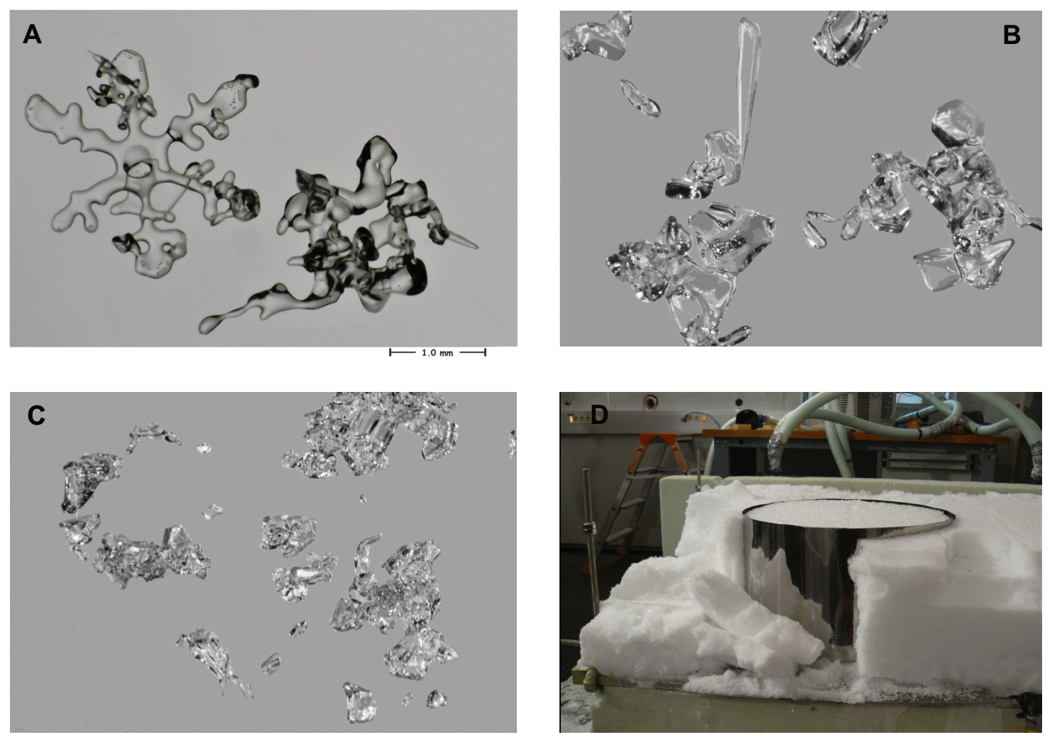
Figure 1(a)–(c) Pictures of snow from S1–S3 taken with a microscope and (d) experimental set-up for S2 sampling. The picture shows the inner part of the temperature gradient box (Calonne et al., 2014a) and the metallic sample holder for the optical measurements.
To sum up, it has been shown that BRF, especially in high absorptive wavelengths, is more sensitive to snow morphology than snow albedo (bi-hemispherical reflectance). Yet no clear relationship has been either established theoretically or evaluated experimentally using optical measurements combined with an objective quantification of the snow microstructure. The objectives of the paper are thus to (i) describe one of the very few datasets that combined measurements of the bidirectional reflectance over the 500–2500 nm range and X-tomography characterization of the snow microstructure, (ii) evaluate the accuracy of the model of Malinka (2014) to simulate the snow BRF and its dependencies on snow microstructure parameters, and (iii) investigate the relationship between bidirectional reflectance and the snow microstructure beyond SSA using both simulation and measurement.
The first section provides a description of the snow samples, the measurement strategy, the optical model, the processing of the X-ray tomography images, and the optical data. The second section presents the results in terms of temporal variability of the snow microstructure, accuracy of the optical measurements, snow microstructure characterization, and model evaluation. Discussions and conclusions are detailed in the last section.
2.1 Experimental set-up and sample description
The general idea of the experiment was to characterize both the snow microstructure and the BRF for the same macroscopic snow sample. The dataset consisted of three macroscopic snow samples: S1 analysed in March 2012 and S2 and S3 analysed in March 2013. S1 consisted of decomposing and fragmented particles/rounded grains (DF/RG) according to the classification of Fierz et al. (2009). S2 was composed of faceted crystals/depth hoar (FC/DH) obtained in a temperature gradient experiment. S3 was taken from the same temperature gradient experiment as S2 except that it was turned upside down so that the grain orientation was changed by 180∘. Under temperature gradient, the facet formation is oriented toward the warmer side of the snow layer. For instance, when the temperature gradient is pointing downward, as is usually the case in nature, the facets tend to form on the downward surfaces while the upward surfaces stay more rounded (see e.g. Figs. 5 and 8 in Calonne et al., 2014a). As a consequence, by flipping S3, the faceted surfaces were oriented upward instead of downward in S2. This was done to investigate the effect of facet orientation on BRF. For each sample, the experiment involved the following steps (see Sect. 2.1.1–2.1.3 for more detail):
-
snow sample preparation,
-
snow microstructure characterization (manual measurements, casting for X-ray analysis) and preparation of a sample for BRF measurements,
-
BRF measurements,
-
snow microstructure characterization (manual measurements, casting for X-ray analysis).
Steps 2 and 4 were performed to characterize the microstructure just before and after the BRF measurements and to control the possible evolution of the microstructure during the BRF measurements.
2.1.1 Snow sample preparation
Figure 1 provides pictures of the snow from each sample. For S1, a 7 cm thick snow layer was collected on a 60 × 60 cm2 styrodur plate after a snowfall close to the lab and stored for 3 weeks in isothermal conditions at −20 ∘C. It then stayed 3 d at −10 ∘C to reach the DF/RG state (Fig. 1a). The objective of this imposed isothermal metamorphism was to obtain a relatively recent snow sample, but with smooth and rounded shapes, that can be resolved at the pixel size we could access with the tomograph (between 6 and 12 µm). For S2 and S3 (Fig. 1b), fresh snow was collected in the field and was sieved into the temperature gradient box from Calonne et al. (2014a) (105 × 58 × 17.5 cm3). A vertical temperature gradient of ≈ 19.4 ∘C m−1 was applied inside the box with a mean temperature of −4 ∘C. Such conditions produce simple structures of large and regular faceted crystals in a reasonable amount of time (Flin and Brzoska, 2008, and Calonne et al., 2014a). Before the measurements were made, S2 and S3 were stored under the described conditions for 16 and 18 d respectively.
2.1.2 Snow sampling and manual characterization
For the BRF measurements, the snow was sampled in a cylindrical sampler with no disturbance of the snow surface as in Dumont et al. (2010) (Fig. 1b). The diameter of the cylinder was 28 ± 1 cm. For S1 the snow thickness was 6.5 cm and for S2 and S3 it was 16.5 cm.
Before this sampling, the snow SSA and density were measured, the SSA with DUFISSS (DUal Frequency Integrating Sphere for Snow SSA measurement; Gallet et al., 2009) and ASSSAP (Alpine/Arctic Snow Specific Surface Area; Arnaud et al., 2011) and the density with manual weighing. The uncertainties on the SSA measured with DUFISSS and ASSSAP are in the range 10 %–15 % for SSA smaller than 60 m2 kg−1 (Gallet et al., 2009; Arnaud et al., 2011). For the density measured by manual weighing, the uncertainties are in the range of 1 % to 6 % (Proksch et al., 2016). Some small near-surface samples were taken for the X-ray analysis and casted using chloronaphthalene (chl) to block snow metamorphism (Flin et al., 2003; Calonne et al., 2014b). These measurements and sampling were reconducted after the optical measurements using the snow sampled in the big cylinder sampler.
2.1.3 X-ray tomography and BRF measurements
For all the samples, the X-ray tomography was performed at 7 µm resolution. Additionally, higher and lower resolutions (5 and 10 µm) were acquired for S1 and S2. The scanned samples were composed of three materials, namely ice, chloronaphthalene (chl), and some residual air bubbles due to incomplete impregnation of the sample (Flin et al., 2003; Hagenmuller et al., 2013). These three materials can be distinguished by their X-ray attenuation coefficient, i.e. their grayscale value I. Table 1 provides an overview of all the images taken for the three samples, and Fig. 2 shows a sub-sample of the 3D images obtained for each sample. The image name provides the sample name, the timing of the scan (B for “before the start of the BRF measurements”, A for “after the end of the BRF measurements”), the location of the sampling ((1) in the centre of the optical sample and (2) on the border of it), and the resolution in microns.
Table 1Summary of all the X-ray tomography images acquired. “B” and “A” refer to “before” and “after” the optical measurement respectively.
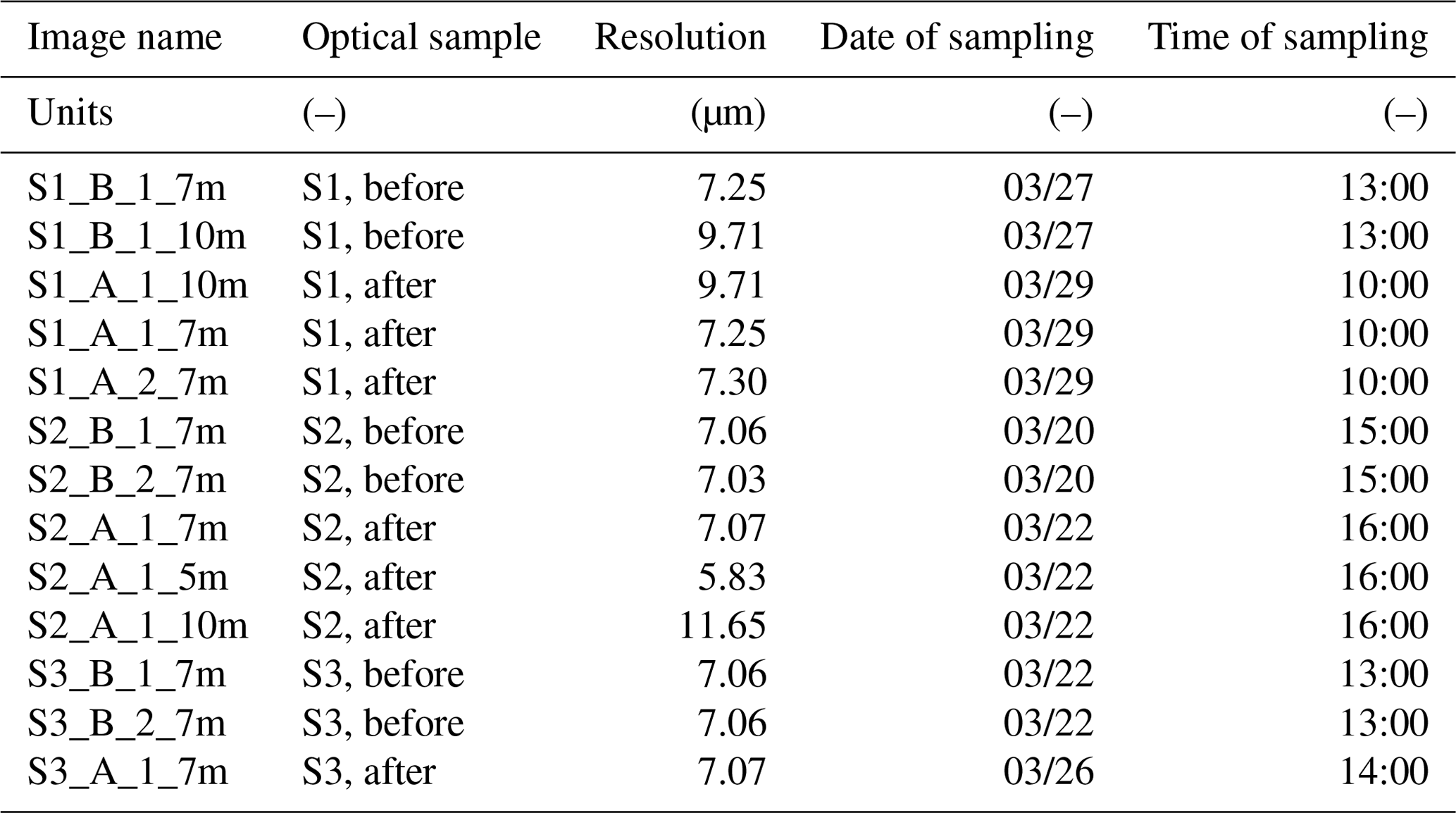
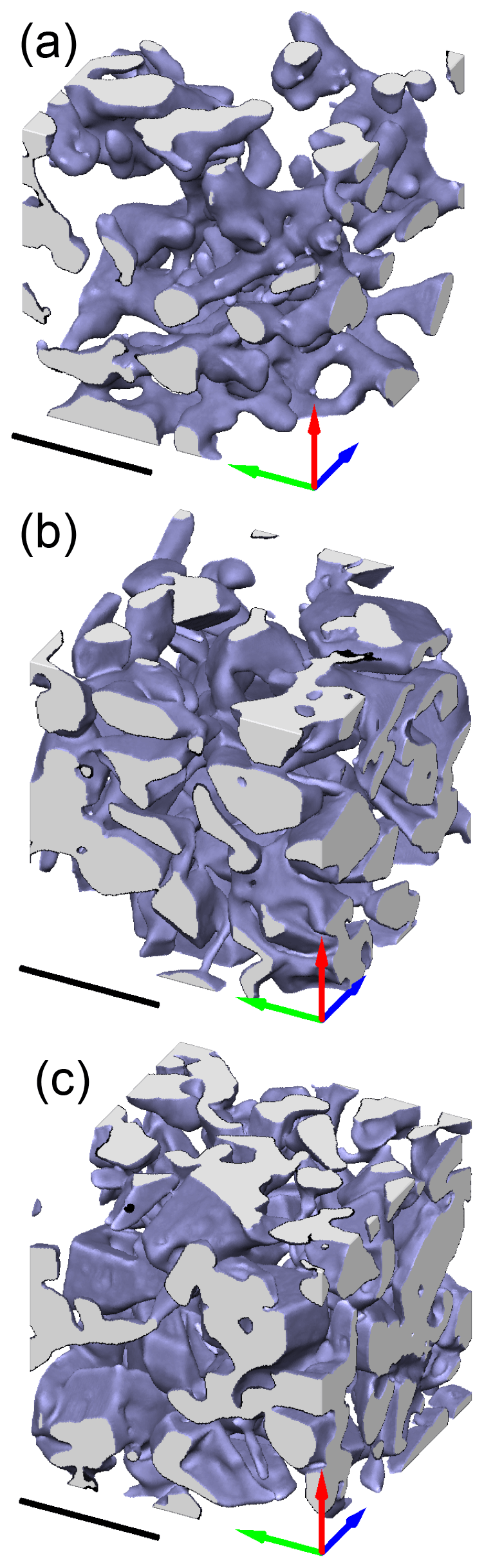
Figure 2Microstructure of the samples S1, S2, and S3 as revealed by X-ray tomography. These visualizations correspond to subsets from the 3D images S1_B_1_7m (a), S2_B_1_7m (b), and S3_B_1_7m (c). The scale bar is 1 mm.
The bidirectional reflectance was measured with a sensor field of view of 2.05∘ using a set-up described in Dumont et al. (2010) and Brissaud et al. (2004) in a cold room at −10 ∘C. The relative accuracy of the bidirectional reflectance distribution function (BRDF) measurements is estimated to be 1 % in Bonnefoy (2001). However, we do not believe that this accuracy is reached for high illumination angles (see Sect. 3.2).
Tables A1, A2, and A3 in Appendix A give an overview of the characteristics of the optical measurements for the three samples. The total duration of the optical measurements was 41 h for S1, 45 h for S2, and 94 h for S3.
2.2 X-ray tomography: image processing and analysis
2.2.1 Image processing
All grey level images were segmented using the following three-step semi-automatic method: (i) pre-processing of the image, including basic beam hardening and ring artefact corrections; (ii) detection of air bubbles and replacement of their levels by the mean grey value of 1-chloronaphthalene (see Flin et al., 2003, 2004, and “METHOD/Threshold-based segmentation/Air bubble detection” in Hagenmuller et al., 2013); and (iii) application of the energy-based binary segmentation method of Hagenmuller et al. (2013), with a resolution parameter r=1.2 voxel.
Once segmented, the obtained binary images can be described in terms of I(X), an indicator function of the ice phase such that
where is a position vector within the sample. Homogeneous cubic subsets of size nmax=700 voxels were then extracted from the original images for further analysis.
2.2.2 Chord length distribution
The chord length distribution (CLD), also called chord length probability density, is often used for the characterization of binary porous media. It is based on a microstructure description in terms of random chords, i.e. iso-phase line segments, whose lengths l are estimated by throwing virtual rays in random directions through the microstructure. The CLD p(i)(l) of phase i denotes the probability p(i)(l)dl of finding a random chord of length between l and l+dl in phase i (Torquato, 2002), thus giving us information on the thicknesses of the elements constituting the considered phase.
In the case of snow, which is known to be an anisotropic material with an orthotropic axis corresponding to the vertical (z) direction (see Calonne et al., 2011, 2012; Löwe et al., 2013; Calonne et al., 2014b, a; Wautier et al., 2015; Srivastava et al., 2016; Wautier et al., 2017), the CLD measured along a particular line depends on its direction. Assuming that the anisotropy is small, we consider the statistical characteristics of a sample in the three Cartesian directions. Namely, the chord lengths were obtained by scanning the segmented images with “rays” along the directions. The z axis is aligned with the vertical direction, while x, y are arbitrarily chosen in the plane perpendicular to the z axis. As the resolution of the X-ray images Δd is finite, the chord length l takes 700 discrete values from Δd to dmax=700Δd along every direction. The total number of chords of length l, , is then used to calculate the CLD of phase (i) in each X-ray image j:
All chords that cross the file borders are inherently dismissed by this estimation method; hence, no hypothesis on the exact nature of the phase (air or ice) outside of the processed image is required. In what follows, the CLDs of the ice phase only are considered. The mean chord length aj and the characteristic function (CF), Lj(α), of the ice phase in X-ray image j are obtained as
where sign 〈〉j denotes averaging in image j. The overall characteristics of the sample are the average over its X-ray images:
where Xj is any metric attributed to image j and N is a number of images of a sample (see Table 1 for the number of images per sample). The sample anisotropy is estimated as
where the subscript means the direction at which chords are taken.
2.2.3 Specific surface area (SSA)
The specific surface area was estimated using two different means: a stereological approach and a voxel projection method. Corresponding quantities calculated with these two methods are indicated with subscripts CLD and VP respectively.
The stereological approach is directly based on the computation of the mean chord length a of the ice phase obtained from the CLD analysis. Indeed, a is uniquely related to the SSA and to the ice volumetric mass ρice by the following formula (see e.g. Torquato, 2002; Malinka, 2014):
The voxel projection estimation, denoted SSAVP, corresponds to an approach developed by Flin et al. (2005, 2011). Based on an adaptive determination of the normal unit vector in each surface voxel, this method allows us to obtain the surface area of the whole object of interest. The SSA can then be obtained after dividing the computed interface area Sint by the associated volume. In the present implementation, a small improvement concerning the computation of the ice phase volume has been added. With the VP method being based on the area estimation of the interface located within a particular voxel (Flin et al., 2005), digitizing divides an image into voxels of two types: ice and air, with the interface voxels being systematically attributed to the ice phase. As a result, the total volume of ice voxels VVP slightly overestimates the true volume of the ice phase Vice by a quantity equal on average to a half volume of the interface voxels Vint. Therefore, SSAVP was computed with the formula
where Sint, VVP, and Vint are computed from the X-ray images. This improved VP method has been validated against several data, including a series of calibrated spheres (see Appendix C).
2.3 Optical measurement analysis
As detailed in Dumont et al. (2010), to convert the spectrogonio-radiometer measurements into BRF values, we divide the measured radiance reflected from the snow surface by the radiance from a reference surface for which spectral albedo and BRF are known. For visible and near-IR wavelengths, the reference surface is a Spectralon® panel. For wavelengths longer than 2440 nm, an infragold® panel is used.
Let be the BRF of a sample under incident zenith angle θi, viewing zenith angle θv, incident azimuth ϕi, viewing azimuth ϕv, and wavelength λ. The reciprocity principle states that
In what follows, we use the anisotropy factor η calculated using the following equation to quantify the anisotropy of the reflectance of a snow sample:
Note that this parameter does not necessarily capture the position of the maximum and minimum reflectances, especially in the visible wavelengths as discussed in Stanton et al. (2016).
2.4 Optical modelling
The model of snow reflectance used in this investigation is described in detail in Malinka (2014) and Malinka et al. (2016). The concept notion used in this model to characterize the snow microstructure is the mean chord length a, which can be seen as the effective snow grain size (Eq. 6). The main quantity that characterizes the optical properties of a snow layer is its optical thickness, τ, which can be calculated as
where β is the volume fraction of ice (1−β is the snow porosity) and H is the sample thickness.
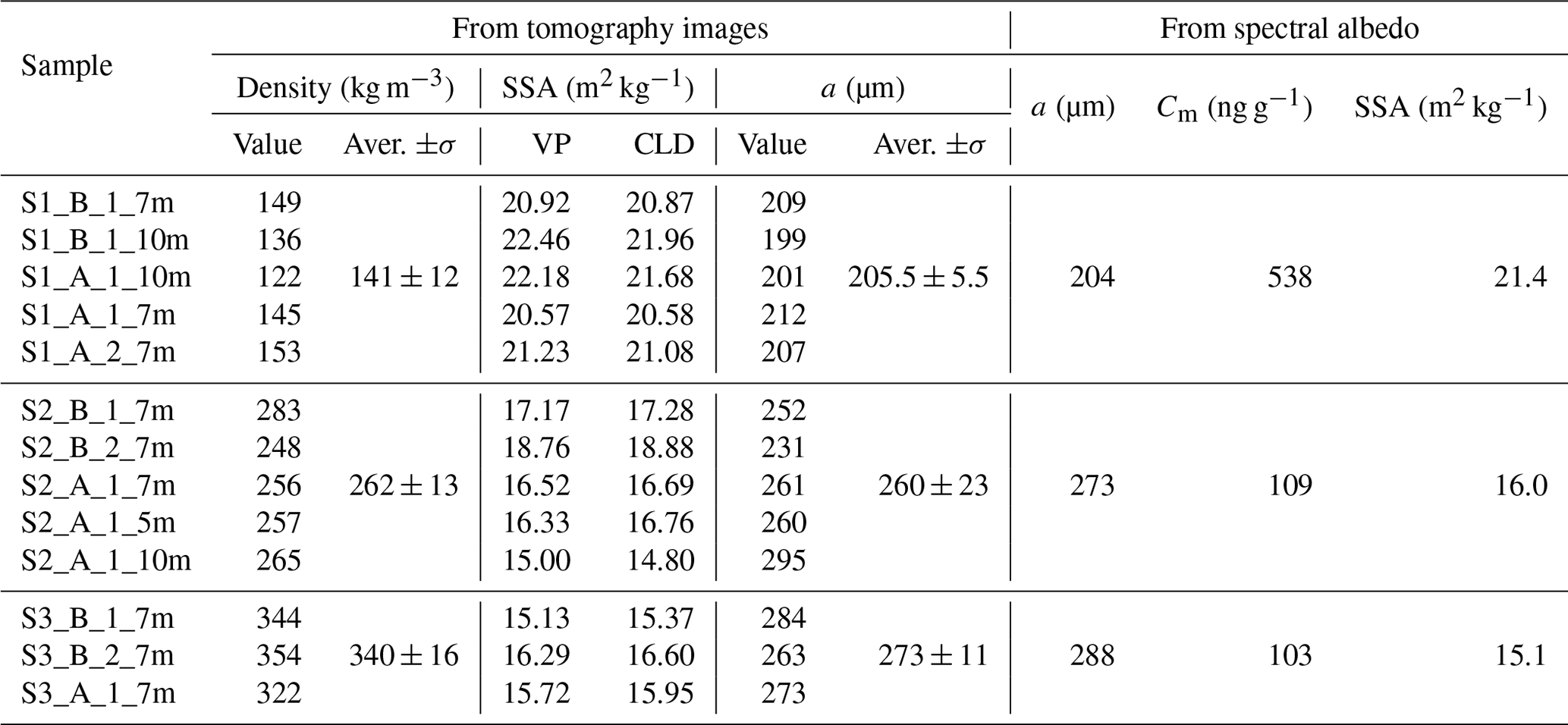
Table 2Sample microphysical properties calculated from the X-ray tomography images and retrieved from the spectral albedo. “B” and “A” refer to “before” and “after” the optical measurement respectively.
Further analysis showed that the albedo calculated with Eq. (10) was strongly overestimated in the green range of the spectrum. In particular, samples S2 and S3 with the geometrical thickness of 16.5 cm have the optical thickness τ calculated with Eq. (10) of greater than 200. According to Malinka et al. (2016) such an optical thickness produces in the green range an albedo of the order of , while the measured quantities reliably show a value of about 0.9. This means that the snow samples contain some light-absorbing particles (Warren, 1982). These particles can be incorporated into the model. When their size is orders of magnitude smaller than that of snow grains (e.g. black carbon), scattering by these particles is negligible in comparison with scattering by snow grains. Thus, the effect of impurities can be modelled as an increase in the absorption coefficient of ice:
where α is the resulting effective absorption coefficient of ice, αice is the absorption coefficient of pure ice, ξ is the particle absorption cross section per its mass (mass absorption cross section), and Cm is the relative mass concentration of absorbing particles. The load and type of impurities were not measured in this experiment, so our choice of a pollutant was quite arbitrary. We assumed that the snow was polluted by black carbon with ξ=11.25 m2 kg−1 at 550 nm, the value recommended by Hadley and Kirchstetter (2012), and spectral dependence given by the inverse of wavelength λ−1 (Bond and Bergstrom, 2006). The impurities internally mixed in the ice phase lead to an increase in the mass absorption efficiency (Flanner et al., 2012; He et al., 2018). The value of 11.25 m2 kg−1 is an intermediate value between fresh BC and internally mixed aged BC (Tuzet et al., 2019, 2020).
The model described in Malinka et al. (2016) uses the three parameters (the optical thickness τ, mean chord length a, and concentration of a contaminant with a predefined spectrum, Cm in our case) to characterize the snow reflectance in full. The more general model of light scattering in porous materials (Malinka, 2014) characterizes the medium microphysical properties via the chord length distribution (CLD). The model of snow in Malinka et al. (2016) assumes exponential CLDs. This model was shown to be reliable in terms of reproducing the measured albedo spectra with the simulated ones in the visible and near-IR ranges (from 350 to 1350 nm). However, in Malinka et al. (2016), there were no direct measurements of the snow microstructure characteristics to verify the model completely. In this work we verify the model by comparing the retrieved mean chord length with that measured directly by the X-ray tomography and investigate the bidirectional reflective properties in a rather wider spectral range (up to 3000 nm), addressing the effect of the µCT-measured CLD vs. the exponential one. To do so, we consider two configurations in the simulation.
-
Assume that the CLD is exponential with the mean values calculated directly from the 3D images (Table 2, col. “Mean chord length, Aver.”). These simulations are labelled EXP hereinafter.
-
Directly use the CLD calculated from the 3D images. The simulations are labelled µCT hereinafter.
For the simulations, we used the database of ice optical properties provided by Warren and Brandt (2008) except when another source is mentioned (Kou et al., 1993, and Grundy and Schmitt, 1998) in Sect. 3.4.
2.5 SSA retrieval from optical measurements
The optical model described in the previous section can be used to retrieve SSA from a measured albedo spectrum. First, the volume fraction of ice β is calculated for a sample:
where ρ is the average sample density taken from the 3D X-ray images. Then the optical thickness τ is calculated by Eq. (10) with an arbitrary starting value of the mean chord length a. After that, the new values of a and Cm are found that provide the best fit, in the least-squares meaning, of the measured albedo spectrum and the simulated spectrum for a given τ calculated using the model from Malinka (2014). The new τ is then calculated by Eq. (10) with the new value of a, and the procedure is repeated until the resulting values no longer change in the first five digits. It usually takes two to three iterations. The SSA and a are related with Eq. (6).
Here we first provide a comparison of the characterization of the snow microstructure obtained with the different methodologies (manual measurements, optical measurements, and X-ray tomography). In a second step, we evaluate the accuracy of the BRF measurements. The last two sections compare the BRF obtained from the model and from the measurements and evaluate the impact of the microstructure on the BRF.
3.1 Snow microstructure
3.1.1 SSA and density
The SSA was obtained by various methods using both optical measurements and X-ray tomography. The optical methods include DUFISSS, ASSSAP, and retrieval from the albedo spectrum (Sect. 2.3). The retrieved values are shown in Table 2 together with the values calculated from the 3D X-ray images. The measured and retrieved albedo spectra of samples S1 and S2 are shown in Fig. 3.
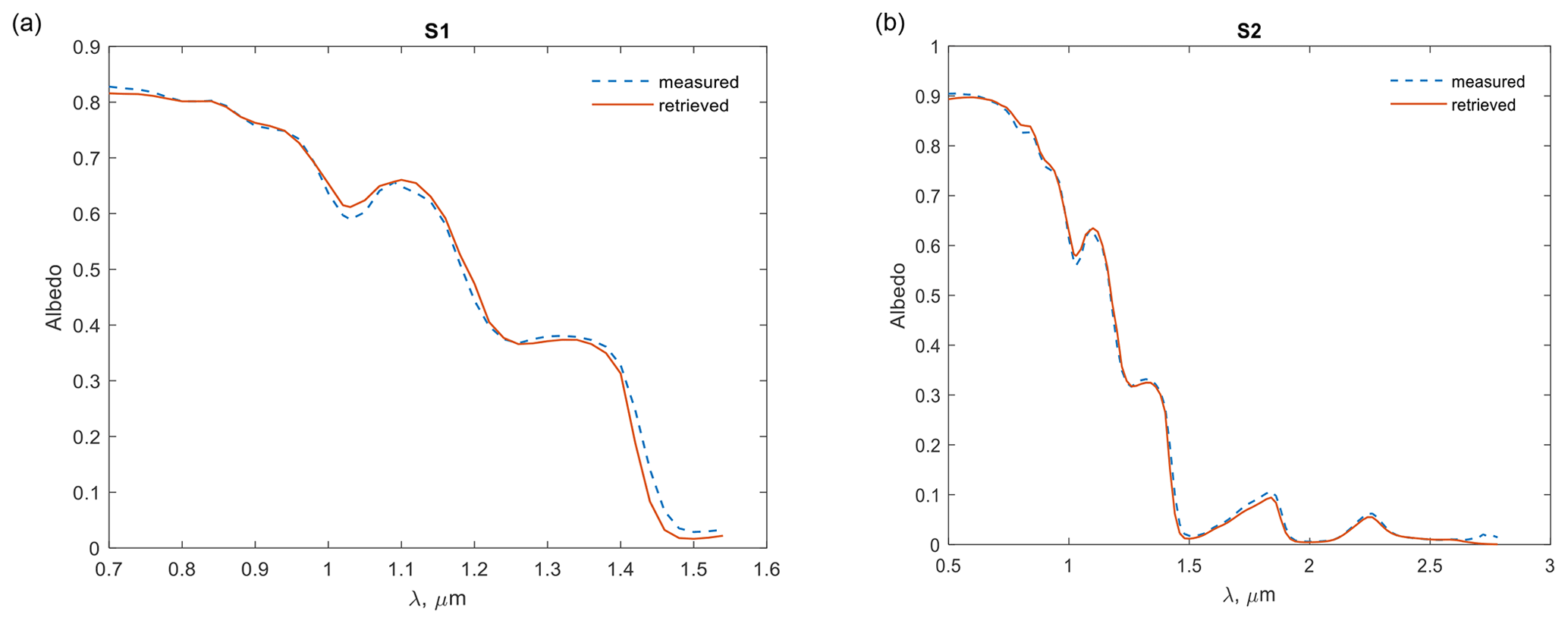
Figure 3Measured and retrieved albedo spectra of samples S1 (a) and S2 (b). The albedo is retrieved following the method described in Sect. 2.5.
Figure 4 compares the SSA values obtained from the 3D images using either the chord length distribution calculation (SSACLD) or the voxel projection method (SSAVP). It shows that the agreement between the two SSA values is good (R2=0.994, RMSE = 0.28 m2 kg−1). The lower SSA values are slightly overestimated via the CLD method, while the higher ones are slightly underestimated. This agreement is to be compared with Fig. 2 in Krol and Löwe (2016a).
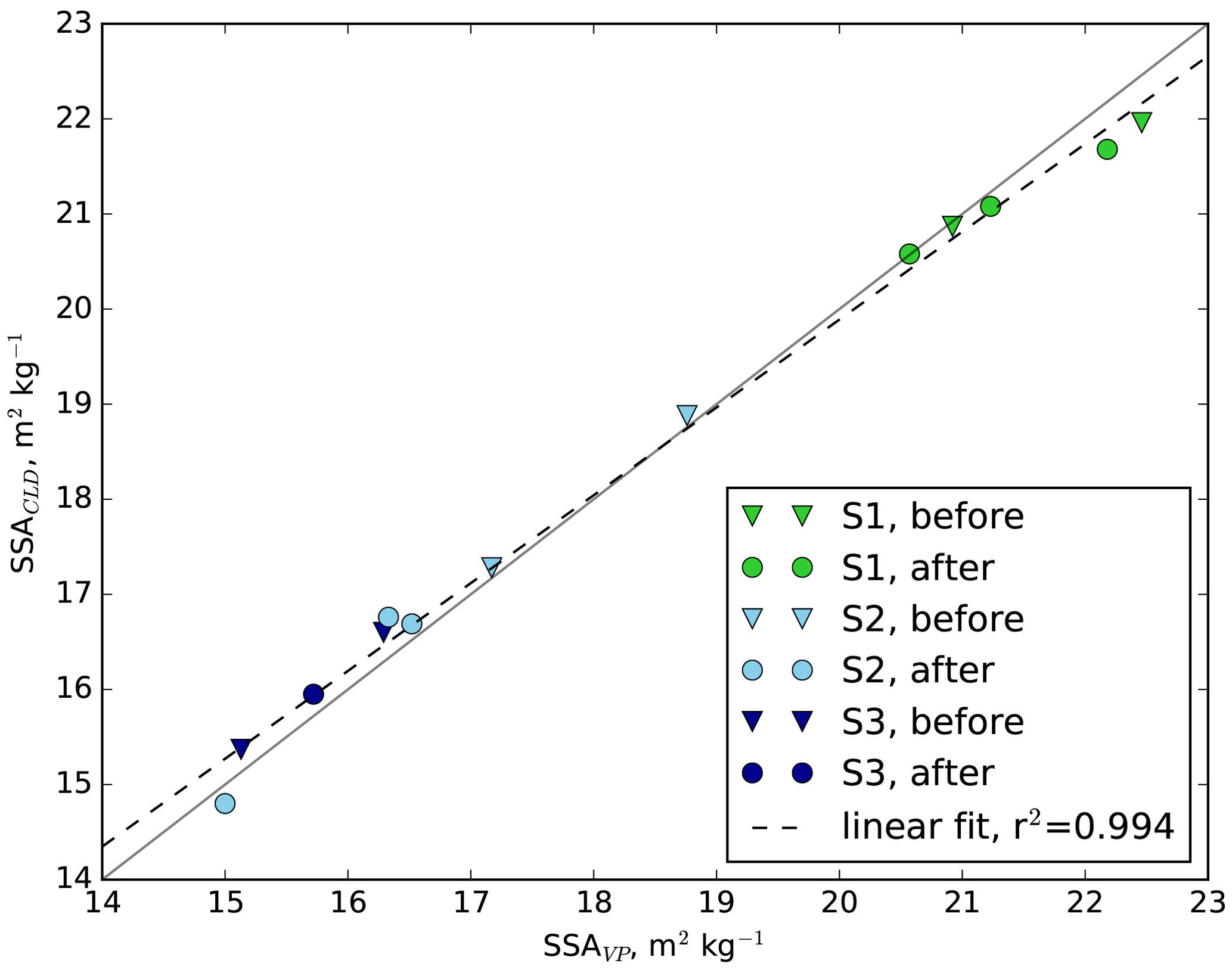
Figure 4SSACLD versus SSAVP in m2 kg−1 computed for all 3D images described in Table 1. The triangle and circles markers indicate that the samples were taken before and after the optical scans respectively. Each marker corresponds to one X-ray image. Each macroscopic sample (S1–S3) is represented by a different colour. The linear fit is represented by the black dashed line.
Figure 5 sums up all the density and SSA measurements performed on all three samples.

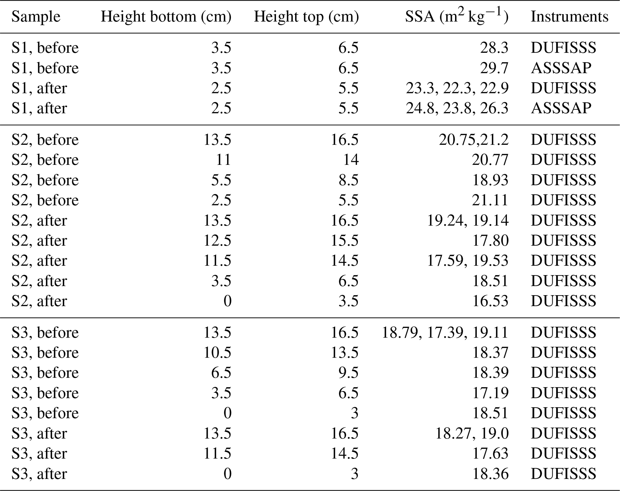
Figure 5Estimated density (first column) and SSA (second column) at various sampling depth in S1, S2, and S3. Values estimated from 3D images are represented by diamonds. Values estimated from measurements (manual weighting for density, DUFISSS, and ASSSAP for SSA) are represented by solid and dotted lines. The SSA retrieved from the spectral albedo is shown with vertical green lines. Values obtained before the optical scan are in blue and after in red. Note that the SSA obtained from 3D images represented in the figure is SSAVP values. The snow surface is represented by the horizontal grey line. Numerical values of all measurements are reported in Tables D1 and D2.
All three samples exhibit some variability both horizontally and vertically. The average density estimated from the 3D images is slightly higher than the manually measured one for S1 and S3 and slightly lower for S2. The average SSA calculated from the X-ray tomography is systematically lower than that estimated from DUFISSS and ASSSAP measurements and is in perfect agreement with the SSA retrieved from the albedo spectra. These discrepancies might be inherent to the methodology but could also be linked to the variation in the properties inside the sample. Note that an X-ray tomography image has a very small size (of the order of several millimetres), the optical measurements with DUFISSS and ASSSAP use surfaces with the size of about 5 cm, and the spectral albedo characterizes a sample as a whole.
Figure 5 shows that S2 and S3 are denser and coarser – i.e. consist of larger grains – than S1 (decomposing and fragmented particles/rounded grains). The density after the BRF measurements is systematically higher than before, and the SSA is systematically smaller (except for one of the S3 measurements). This indicates that the snow microstructure as a whole has slightly evolved during the BRF measurements: snow has become denser and coarser (possibly because of sublimation in the cold room). This is to keep in mind when analysing the optical measurements. S1 exhibits larger changes in SSA than S2, and S2, in turn, demonstrates larger changes than S3. This is compatible with the fact that snow with lower density and higher SSA is subject to more rapid evolution (e.g. Flin et al., 2004; Carmagnola et al., 2014; Schleef et al., 2014). Also, the retrieval has shown that the snow taken in the mountains (S2 and S3) was much more pure: the soot concentration in it was 5 times less than that in the snow taken in the urban area (S1) (Table 2).
3.1.2 CLD analysis
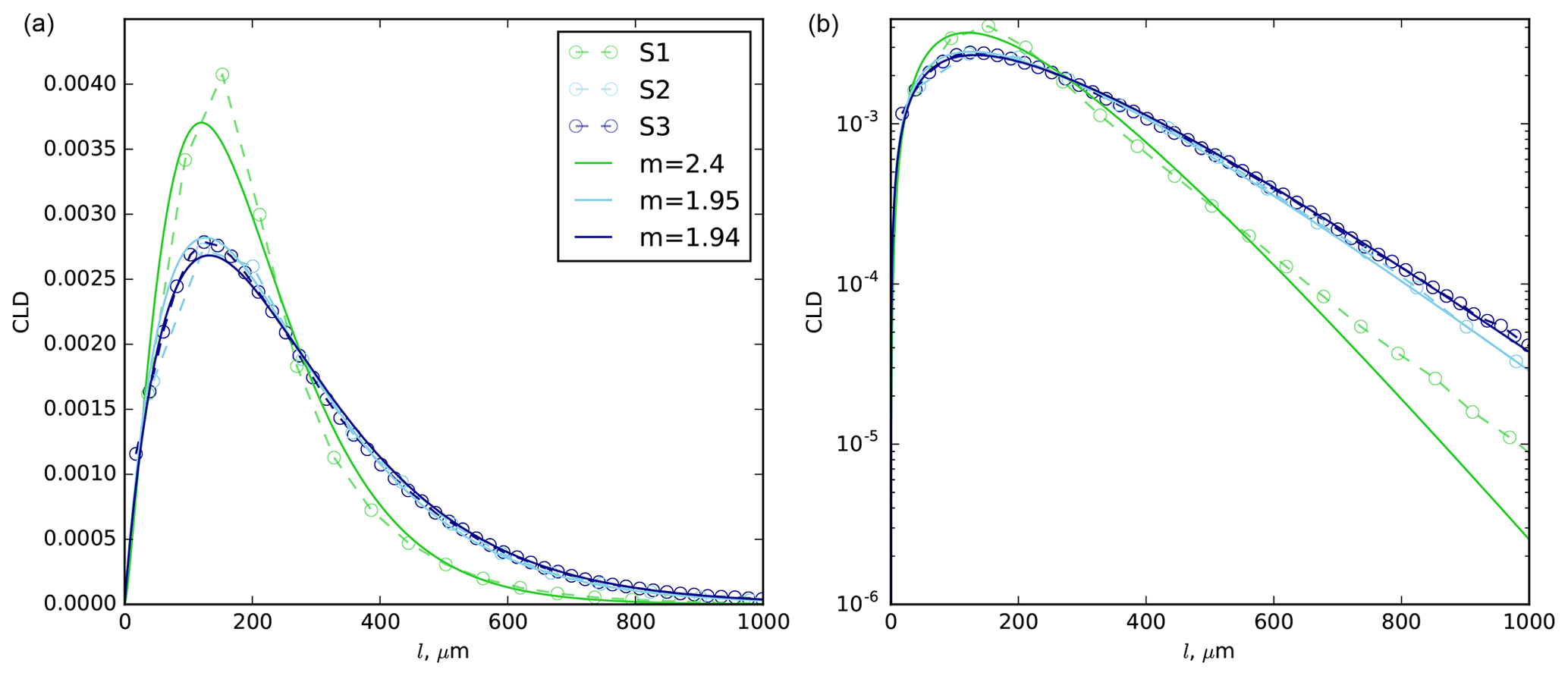
Figure 6 compares the CLD of the three samples estimated from all the images. S1’s CLD is narrower than S2's and S3s' CLD; however, all of them exhibit similar features. They have almost exponential tales for large l and approach zero at l=0. The latter fact means the ice–air interface does not have edges at the image resolution for the three snow samples, in contrast, e.g. to a set of random polyhedra, which has a Markov property, i.e. the exponential CLD. Distributions of this type can be represented by the gamma distribution:
where a is an average, Γ(m) is the gamma function, and m is a shape parameter. The exponential distribution is a particular case of the gamma distribution with m=1. Thus, the shape parameter m indicates the deviation of a distribution of this type from the exponential one. Fitted gamma distributions are also indicated in Fig. 6 (see below for the calculation of the value of m).
The CLD determines optical properties of a mixture not explicitly but via its Laplace transform (Malinka, 2014), which by definition is the characteristic function of the distribution, L(α) (see Eq. 3).
If the argument α is equal to the substance absorption coefficient, then the characteristic function L(α) describes the process of photon absorption while travelling along random chords within an absorbing material, in this case ice (see Malinka, 2014). The Laplace transform of the gamma distribution (Eq. 13) is
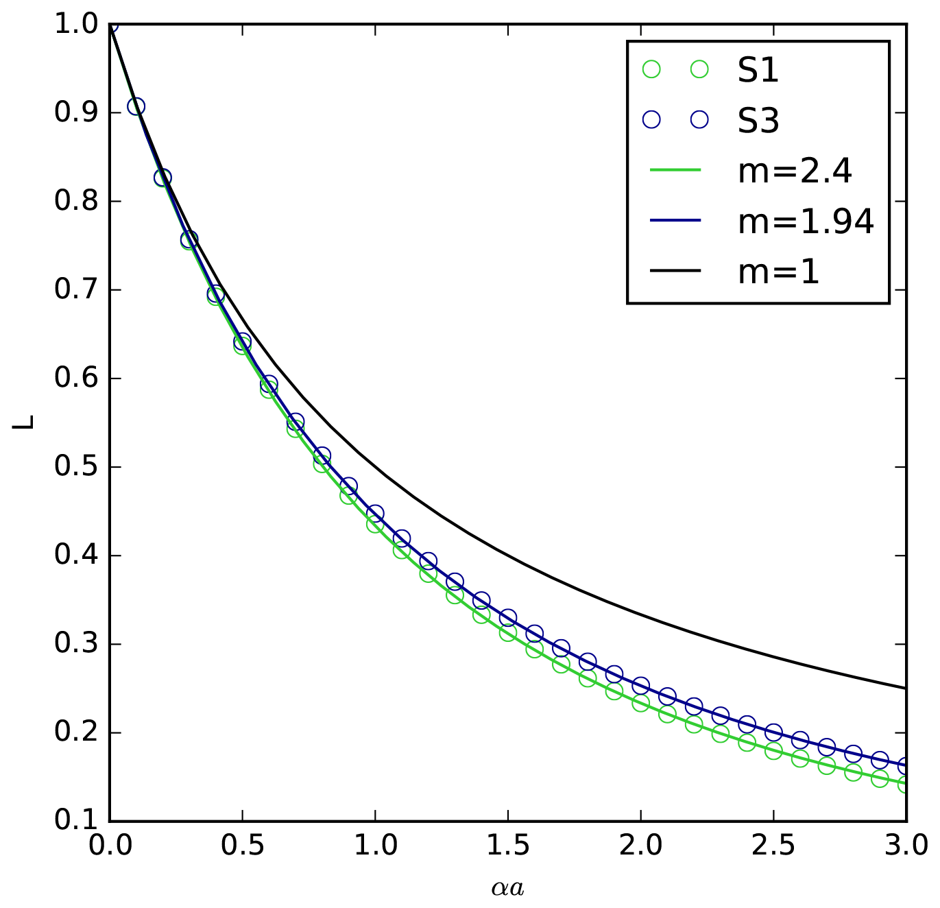
Figure 7µCT-measured characteristic functions for S1 and S3 and their approximations with the Laplace transform of the gamma distribution with different shape parameters m. All the images have been used for S1 and S3. S2 is not shown because of the overlap with S3.
Figure 7 shows the characteristic functions calculated directly from the 3D images of S1 and S3 using Eq. 3 and their approximations with the Laplace transforms (Eq. 15) of the gamma distribution with m calculated by least-squares fitting. The Laplace transform of the exponential distribution (m=1) is shown for comparison. The characteristic function of S2 is not shown because of the overlap with that of S3.
The characteristic functions calculated directly from the X-ray images at large values of argument αa could be distorted by the image discretization. Their values are reliable if the error of the argument αa due to the discretization is small. If the image resolution is Δd, then the condition Δd≪1 should hold true. If the resolution is 7 µm and the mean chord is about 200 µm, we have
i.e. αΔd<0.1 for αa<3, so the µCT-measured characteristic functions presented in Fig. 7 are not affected by the discretization error.
The characteristic function in Eq. (3) has the power series expansion
where μ2 is the second moment of the CLD.
The exponential CLD has the Laplace transform from Eq. (15) with m=1, hence the expansion
Comparing the second-order term in Eq. (18) with that in the general expansion in Eq. (17), we find that the deviation of the CLD from the experimental law, in general, can be characterized by the value (Krol and Löwe, 2016a) or its deviation from unity, δ:
For the gamma distribution this value is expressed via the shape parameter as follows:
The deviations from the exponential law δ, calculated from m values with Eq. (20) and directly from the CLD with Eq. (19), are shown in Table 3. The values obtained in this experiment are slightly higher but consistent with the results of the analysis of Krol and Löwe (2016a).

The deviation of the CLD from the exponential law matters, i.e. affects the optical properties, if the difference between Eqs. (17) and (18) is not negligible, i.e. .
Thus, the absorption at which the deviation matters can be estimated as
Provided a∼200 µm and δ∼0.25, we get α∼104 m−1. So, we can expect that the true shape of the CLD will impact the optical properties only at very high absorptions. The absorption coefficient of ice in the range 500–2500 nm approaches such values at 1500, 2000, and 2500 nm (see below). At these absorptions, for which αa∼2 , we can expect that the light penetration depth will not exceed the mean chord length a, treated as the effective snow grain size, so all the incident light will be absorbed within the skin layer – a layer at the surface with a thickness of “one grain”. The reflectance will be completely determined with Fresnel reflection by crystal facets and refraction by fine grains in this skin layer. Under these conditions, the fine grains, and therefore the CLD behaviour at small lengths, will play a more important role. The facet orientation at the surface can differ from that in deeper layers as well.
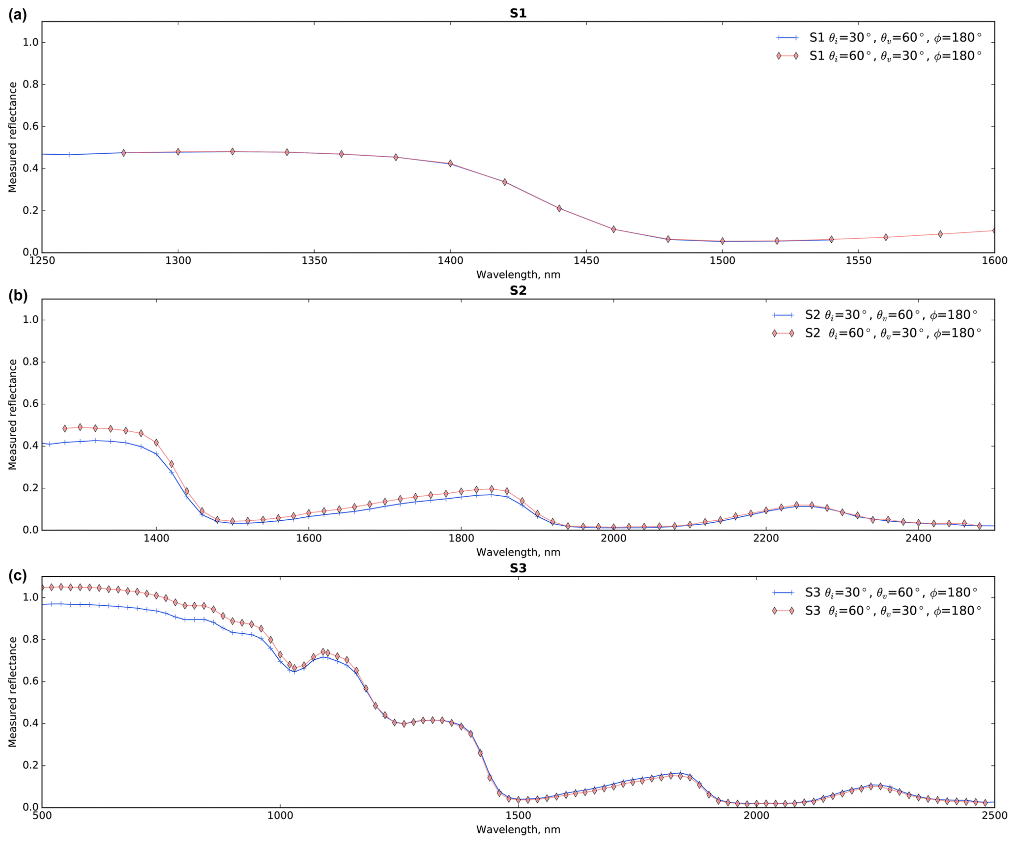
Figure 8Measured reflectances of the three samples (each panel) obtained for optically equivalent geometries.

Figure 9Measured (circles) and modelled (curves) BRF for the three samples (S1: a, S2: b, S3: c) for , , and . The solid and dashed curves correspond to the simulated reflectance using the snow microstructure measured before and after the optical measurements respectively. All the simulations were performed with the exponential CLD. The differences between the measured and simulated reflectances are reported on the right y axis with crosses and dots. The 3D images at 7 µm resolution, i.e. three images per sample, are used for the simulations.
3.2 Optical measurement accuracy: reciprocity principle
Figure 8 compares the reflectances obtained for optically equivalent geometries according to Eq. (8). For S1, Eq. (8) is really well verified. This is not the case for S2 and S3, especially in the visible range. The SSA temporal evolution during the BRF measurements (see Fig. 5 in Sect. 3.1.1) cannot explain these discrepancies, since it would result in a decrease in reflectance in the measurements taken later, so that the red curves would be lower than the blue ones, but the contrary is observed. A possible explanation lies in the fact that the illumination pattern is larger in the sample holder for large incidence angles (e.g. 60∘). Since the snow does not perfectly fill the sample holder, direct reflection of light coming in on the side of the sample holder to snow cannot be avoided, acting as an additional source of light and contributing to the reflected signal. This hypothesis is reinforced when comparing other equivalent geometries (θi=0∘, θv=30∘) showing almost perfect agreement between the two reflectances. This indicates that reflectances measured for θi=60∘ should be analysed accounting for the fact that they might be overestimated because of re-illumination, especially for low absorptive wavelengths.
This shows that the relative accuracy of the measurements estimated at 1 % in Brissaud et al. (2004) is not reached for high illumination angles. In the following, the interpretation of the BRDF measurements is mostly restricted to wavelengths larger than 800 nm and – except in Sect. 3.4 – to an illumination angle of 30∘ to minimize this effect. For wavelengths larger than 800 nm, the effect of the limited thickness of the sample and of the presence of light-absorbing impurities (Warren, 1982) is also limited.
3.3 Model vs. measurements
3.3.1 Spectral variations
Figure 9 compares the measured and simulated spectral reflectances for all three samples. The results show that the simulated reflectances generally agree well (absolute difference less than 0.02) except for several wavelength ranges that exhibit systematic bias for all three samples. There is a little BRF overestimation in the visible and near-IR ranges up to 1400 nm. Nevertheless, the albedo does not demonstrate any overestimation in this range of wavelengths. The BRF is overestimated mainly at oblique incidence and viewing angles and only in the visible range (see also Figs. 13, B3, and B4). We attribute the overestimation either to shortcomings of the measurements due to geometry (see above) or to the drawbacks of the model in the description of the angular dependence of the bidirectional reflectance, which may not take into account several factors, such as dense packing or surface roughness. There are some peaks of the difference – 1000, 1200, and 1450 nm – where the reflectance, following ice absorption, has steep changes. However, the most pronounced differences are in the ranges 1400–1900 and 2150–2300 nm. These differences are especially pronounced for S1. We relate these differences to the difficulties of the measurements of ice absorption in these ranges with high accuracy.
To examine this effect, we simulate the snow reflectance in the most pronounced difference range 1400–1900 nm using the values of the complex refractive index of ice taken from different databases. Figure 10 compares the measured and the simulated reflectances in this range for S1 and S2, using several databases of the complex refractive index of ice: Warren (1984), Kou et al. (1993), Grundy and Schmitt (1998), and Warren and Brandt (2008). For S1 both the incidence and observation angles are 60∘. For S2 the observation angle is 60∘, but the incident angle is taken as 30∘, because of the problems discussed in Sect. 3.2. As seen from Fig. 9, the data from Grundy and Schmitt (1998) provide the simulated values closest to the measured ones and will be used in further simulations for this spectral region. However, as far as we understand, the additional careful measurements of the complex refractive index of ice in the IR range are still needed.
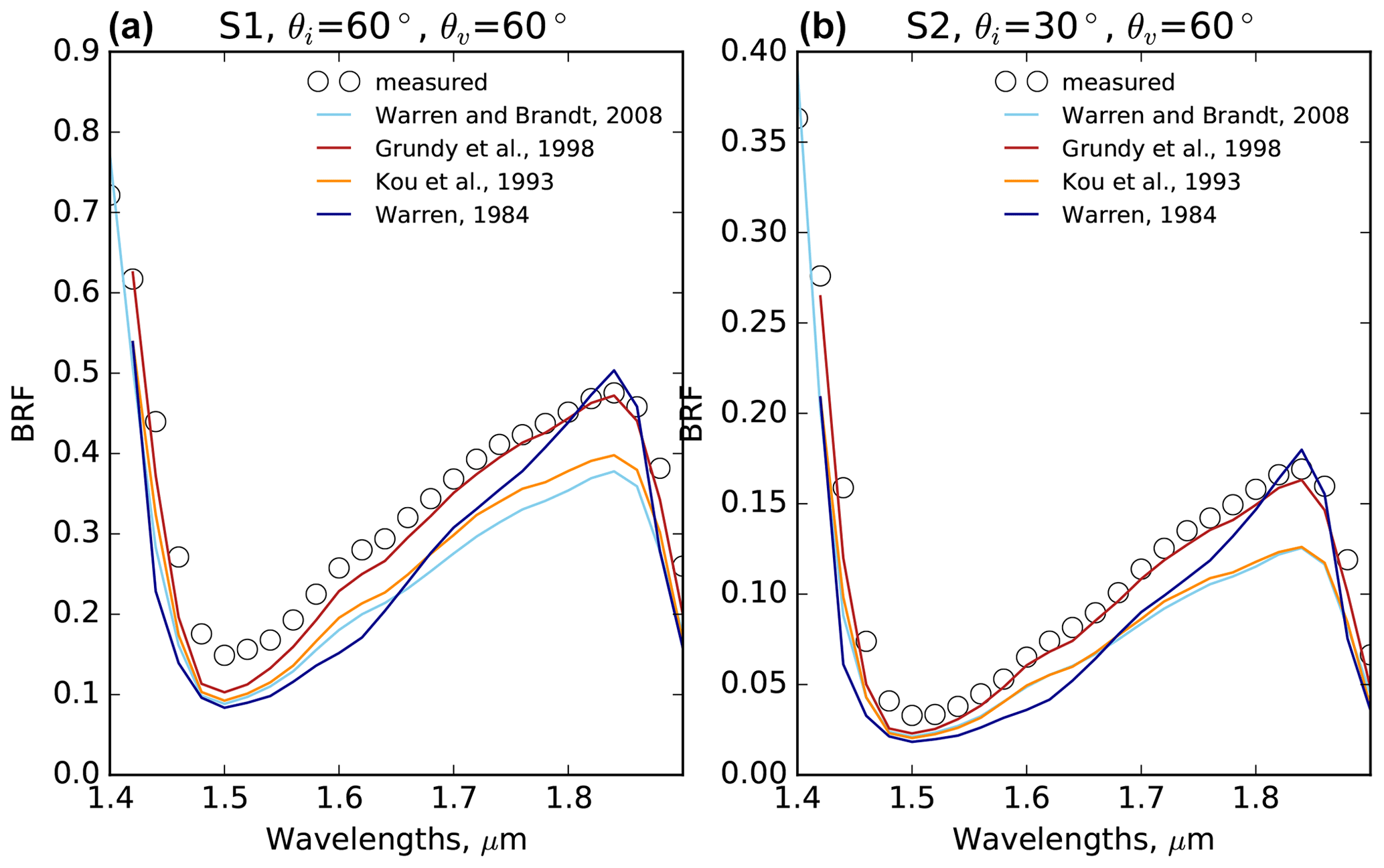
Figure 10Measured (circles) and simulated (EXP, lines) reflectances in the principal plane for S1 (a) and S2 (b) in the 1400–1900 nm range. The incident zenith angles are 60∘ for S1 and 30∘ for S2. The viewing angle is 60∘ zenith and 180∘ azimuth. The BRF has been simulated using different ice refractive index databases: Warren and Brandt (2008) (light blue), Warren (1984) (dark blue), Grundy and Schmitt (1998) (red), and Kou et al. (1993) (orange).
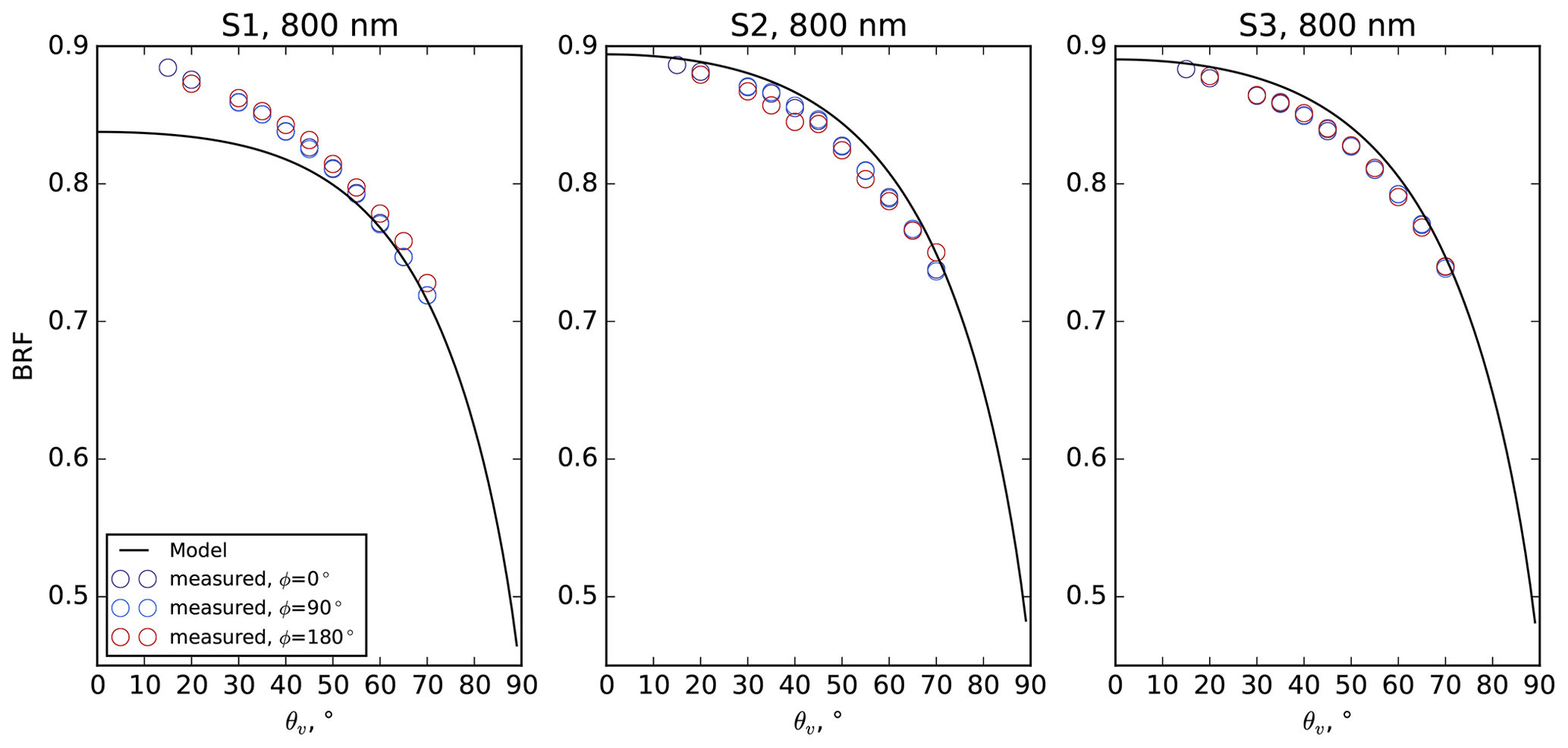
Figure 11Measured (circles) and simulated (EXP) (curves) BRF of the three samples at vertical incidence at 800 nm.
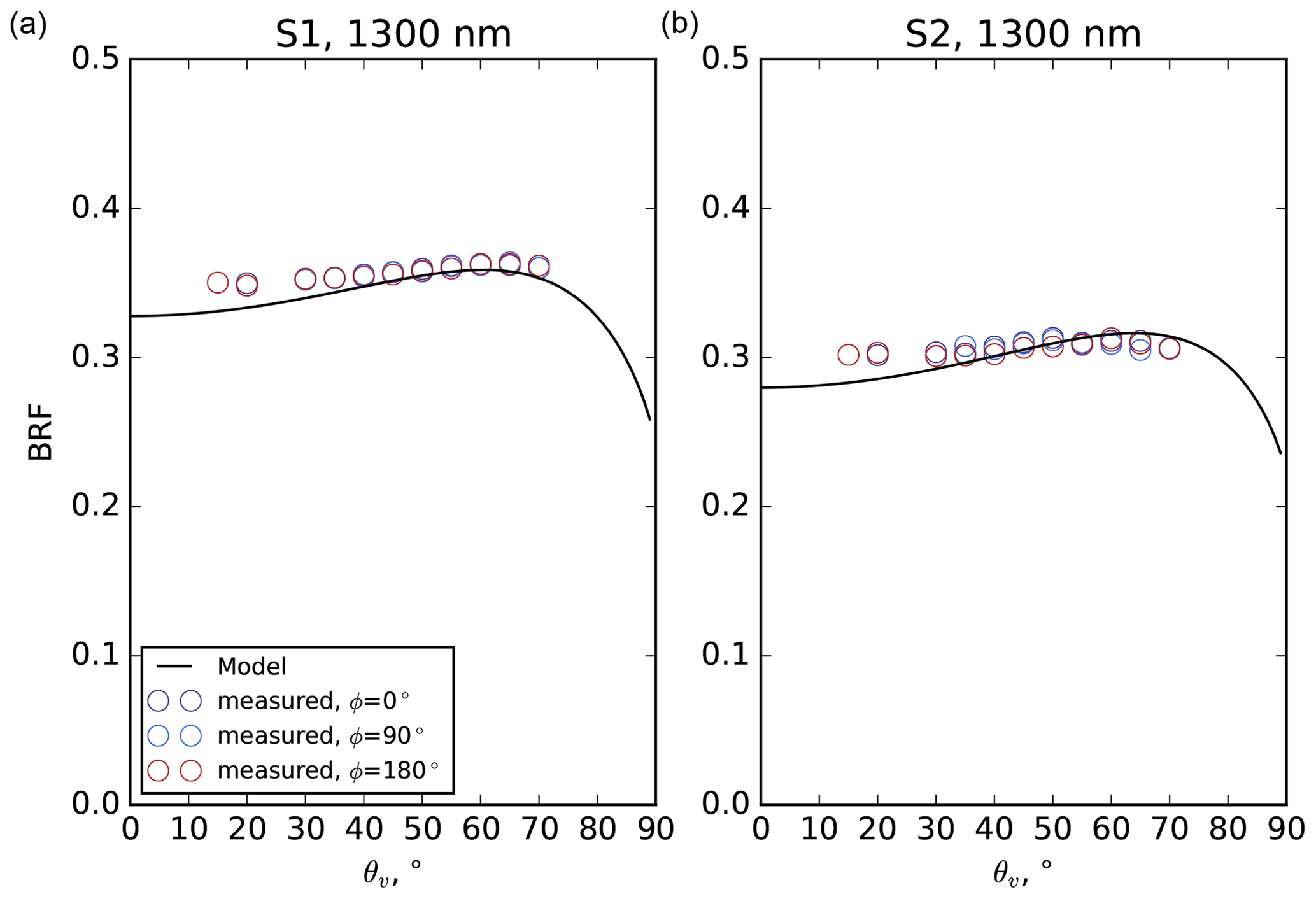
Figure 12Measured (circles) and simulated (EXP, curves) BRF for S1 (a) and S2 (b) at vertical incidence at 1300 nm.
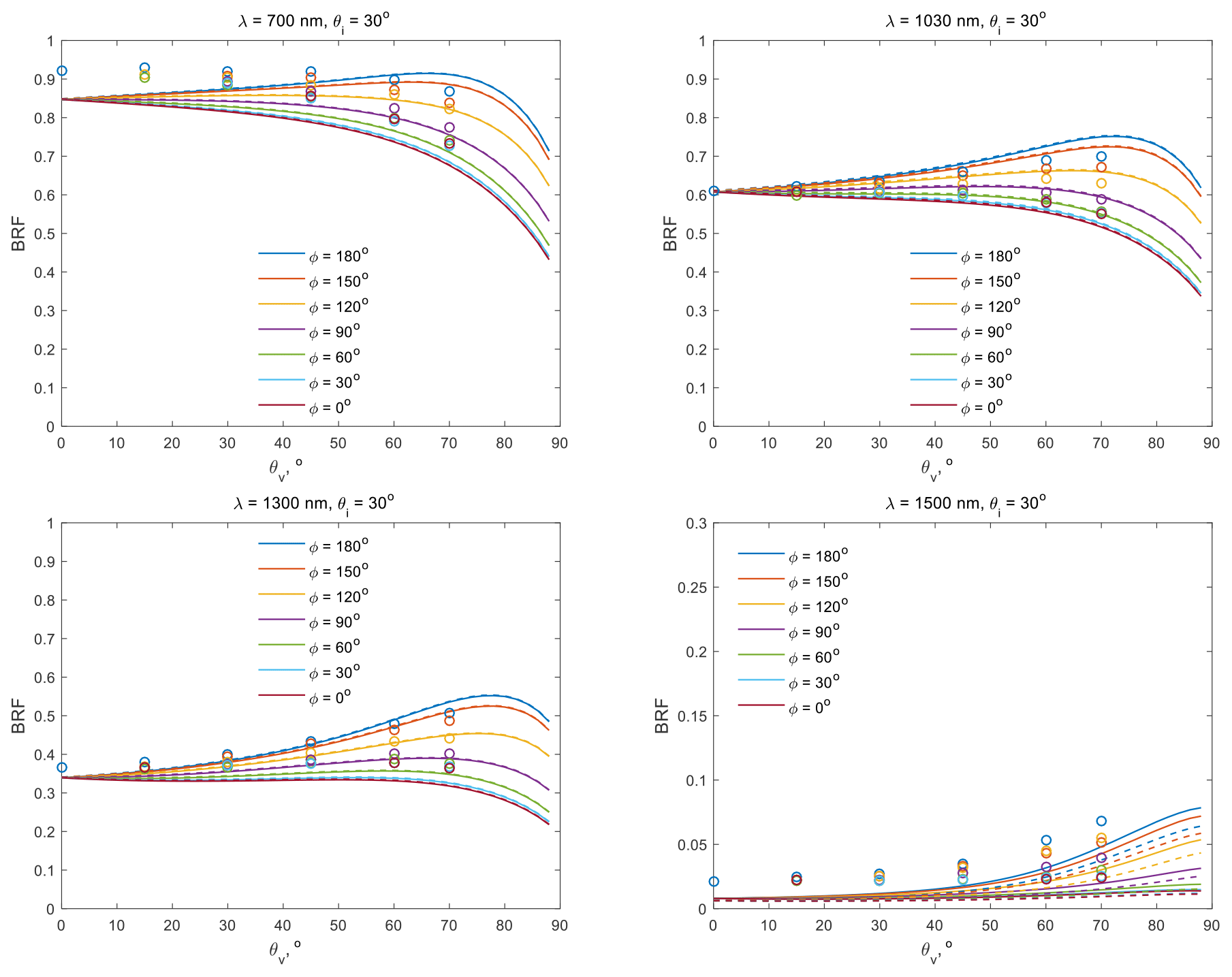
Figure 13BRF measured (circles) and simulated with the exponential (curves) and µCT-retrieved (dashes) CLDs for S1 at 700, 1030, 1300, and 1500 nm. The incident zenith angle is 30∘. The different colours correspond to the azimuth. The µCT-retrieved CLDs are averaged across all of the S1 X-ray images.
3.3.2 Angular distribution
Figures 11 and 12 compare the simulated and measured BRF at vertical incidence for 800 and 1300 nm. The simulated and measured data agree well, except for S1 at the observation directions close to vertical. Figure 13 shows the simulated and measured BRF at 30∘ incidence for a wide range of the observation angles. Except at 1500 nm, the simulated BRF generally agrees with measured values. However, for high viewing zenith angle, typically higher than 45∘, the simulated anisotropy is stronger than the measured one. These conclusions hold for S2 and S3 (see Figs. B3 and B4 in the appendices). At 1500 nm, the simulated BRF is lower than the measured values, as already reported in Fig. 9. The discrepancies between the simulated and measured BRF are generally greater than the spread in the simulation due to the variability of the snow microstructure (different images).
Figures 14, B1, and B2 (see Appendices) compare the measured and simulated angular distribution of reflectance for three wavelengths (1320, 800, and 1500 nm), for an incident zenith angle of 30∘ and for the two configurations of simulations (EXP and µCT).
Figure 14 is obtained for 1320 m (wavelength with medium absorption). It shows that (i) the angular pattern and reflectance magnitude are reasonably reproduced by the model and (ii) there are no detectable differences between the EXP and the µCT simulations. It also shows that the higher reflectance values are obtained for S1 and the lower for S3, which is consistent with the SSA of the samples. The third line of Fig. 14 demonstrates that for the three samples, the simulated reflectance is overestimated in the forward scattering direction and underestimated in the backward direction, so at 1320 nm, the model seems to overestimate the anisotropy of the reflected radiation. The conclusions obtained at 1320 nm also stand at 800 nm (low absorption, Fig. B1). The possible causes of this general overestimation of the anisotropy of the angular pattern are discussed in Sect. 4. However at 1500 nm (high absorption, Fig. B2), the reflectance is underestimated almost twice for all angles and all samples in the simulations. The reflectances for this wavelength are very low and can also be affected by experimental uncertainties. Stronger differences in reflectances at 1500 nm are noticeable between the samples and also between the EXP and µCT simulations.
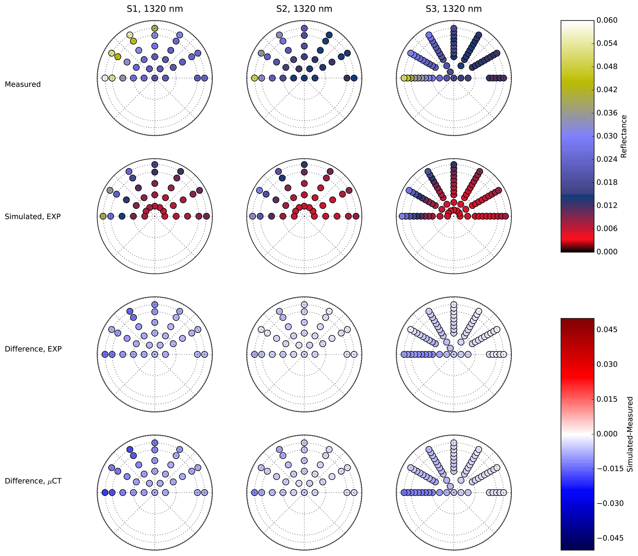
Figure 14Measured (first line) and simulated (second line) reflectances for the three samples (three columns) at 1320 nm. The incident zenith angle is 30∘. On the polar plot, the polar angle represents the azimuth, and the radius is proportional to the viewing angles. The dotted circles represent viewing angles of 30, 60, and 70∘. The two lower lines represent the difference between the simulated and measured reflectance for the exponential and µCT-retrieved CLDs. The images used for the simulations are S1_E_1_7m, S2_B_1_7m, and S3_B_1_7m. .
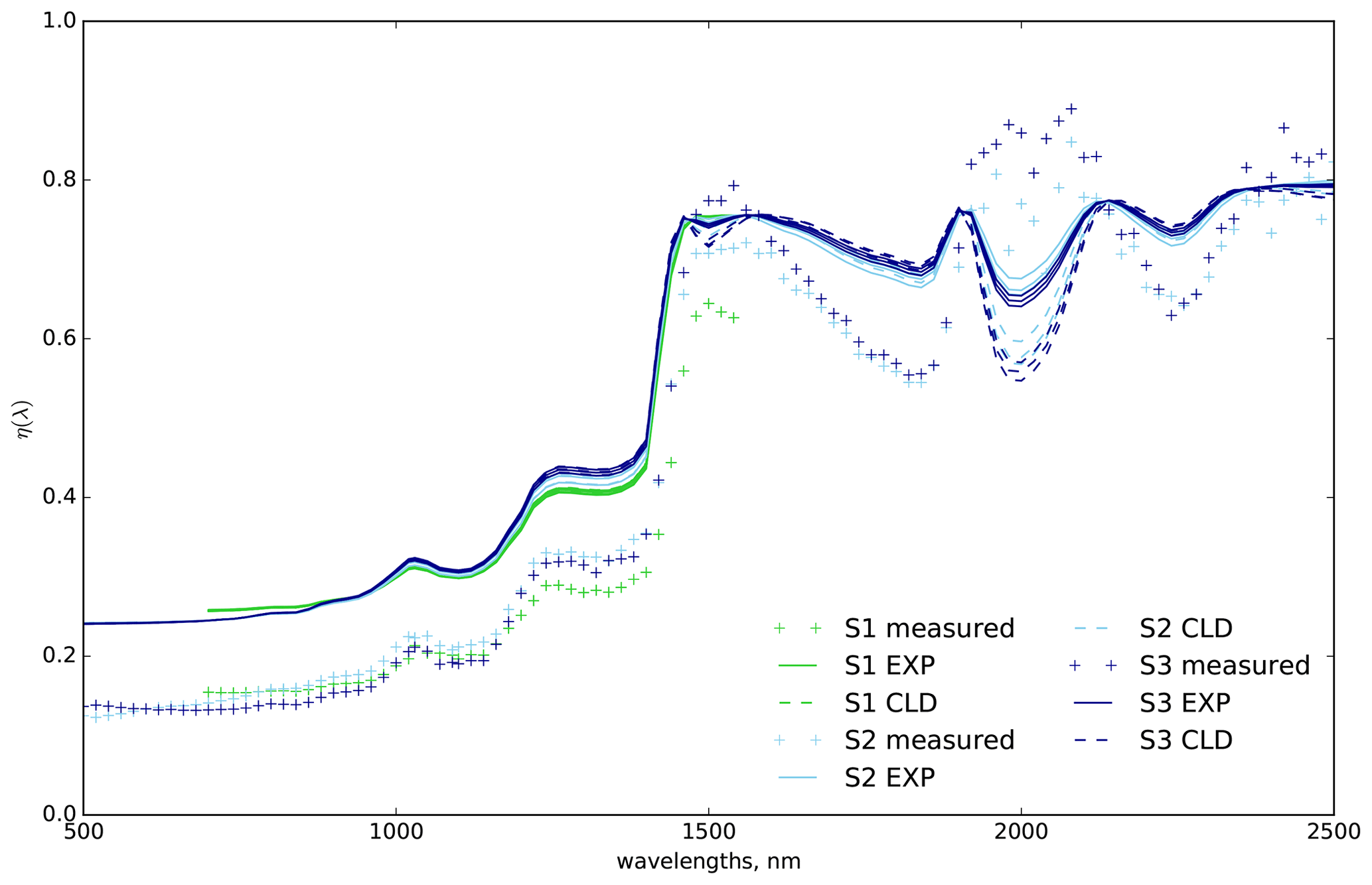
Figure 15Measured (crosses) and simulated (dotted curves for µCT and solid curves for EXP) values of parameter η (Eq. 9) obtained for the three samples. All the images were used for the simulations.
Figure 15 compares the anisotropy of the reflectance measured and simulated quantified by the anisotropy parameter η (Eq. 9). It shows that η is higher in the simulations than in the measurements, except for highly absorptive wavelengths (around 1500 and 2000 nm), where the differences between the samples are higher in the measurements than in the model. Also, the EXP and µCT simulations only differ for these highly absorptive wavelengths. This general overestimation of the anisotropy in the simulations is also visible in Figs. 9, 13, 14, B1, B2, B3, and B4.

Figure 16Measured (markers) and simulated (lines) reflectance in the principal plane (forward direction) for an incident zenith angle of 60∘ at 1280, 1420, 1500, and 2000 nm. Plain lines correspond to EXP and dotted lines to µCT simulations. All images have been used as inputs for the simulations. The red and orange lines correspond to simulation obtained for S1 with refractive index from Grundy and Schmitt (1998) and Kou et al. (1993). For all the other simulations we used refractive index from Warren and Brandt (2008) .
3.4 Results at 60∘ illumination angle
Figure 16 compares the measured and simulated reflectance in the principal plane (forward direction) for an incident angle of 60∘ at several wavelengths. At high viewing angles, for all wavelengths and despite the lower SSA, S3 exhibits higher reflectance than S2 and S1. The higher the absorption, the more pronounced this effect, so it might be related to the facet orientation at the surface. At 1280 nm, the simulations and the measurements agree well, with a slight overestimation of the reflectance at high viewing angles. For the other wavelengths, the model generally underestimates reflectance. The use of alternative ice refractive index values (Grundy and Schmitt, 1998) improves the simulations at 1420 and 1500 nm but is not sufficient to reconcile the measurements and the simulations for high viewing angles at 1500 and 2000 nm (see Sect. 4 for additional discussion). The difference between the µCT and EXP simulations is only noticeable for high viewing angles and high absorption. Under these conditions, accounting for the CLD shape retrieved from µCT leads to a decrease in the calculated reflectance in comparison with the simulations with exponential CLD.
This study presents a dataset that combines the snow bidirectional reflectance over the 500–2500 nm range with different illumination geometries and 3D images of snow using X-ray tomography, which allows analysis of the snow microstructure, e.g. its SSA and density. The SSA is calculated using two different methods: the voxel projection method (VP) and the method based on the ice chord length distribution (CLD). The comparison between the two SSA values is in excellent agreement (R2=0.994). The SSA and mean chord values computed from 3D images are generally lower than those obtained via DUFISSS and ASSSAP optical methods and in excellent agreement with those retrieved via spectral albedo. The comparison between density values obtained via the 3D images and via manual measurements exhibits slightly higher density for 3D images, which might relate to the heterogeneity of the samples and to the segmentation process applied to the images (see Fig. 12 in Hagenmuller et al., 2013). The analysis of the 3D images has shown that the CLDs approach zero at l=0 both in the DF/RG snow and in the snow after long evolution in temperature gradient conditions. This means that the air–ice interface is smooth and has no sharp edges even though faceted crystals are present, at least for the images considered in this study. A possible reason for this is the continued curvature-driven metamorphism of snow, which already begins during a snowfall (Flin et al., 2003; Brzoska et al., 2008; Krol and Löwe, 2016b).
The analysis of the characteristic functions of random chords in the snow phase calculated directly from the 3D images has shown that the random chords obey the gamma distribution with the shape parameter m, equal to 2.40, 1.95, and 1.94 for S1, S2, and S3 respectively. The deviation of the distribution from the exponential one is the lowest for the more faceted crystals (sample 3) and the highest for DF/RG (sample 1). Its values, however, largely vary for the same macroscopic sample probably due to both the temporal evolution and the snow heterogeneity. The deviation values are slightly higher but in the same range as obtained by Krol and Löwe (2016a).
The comparison between the simulated and measured reflectance under a specific geometry ( or 60∘, and ) shown in Fig. 9 demonstrated that the simulated values generally agree well (absolute difference lower than 0.03) over the whole spectrum 500–2500 nm and that for this geometry the impact of the CLD is small. Systematic differences are found in several wavelength ranges. Such discrepancies have already been reported in several studies (e.g. Carmagnola et al., 2013) and attributed to uncertainties in the values of the ice complex refractive index from Warren and Brandt (2008). The use of alternative databases, especially the one from Grundy and Schmitt (1998) noticeably improves the agreement in the range 1400–1500 nm as shown by Fig. 10. A more extensive comparison of the simulated and measured reflectance angular distribution at 30∘ illumination angle shows that the BRF predicted by the model is in good agreement with the measured one. Spectral changes in the angular distribution are well reproduced. The impact of the CLD shape on the simulation is only detectable for absorptive wavelengths (1500 nm) and high viewing zenith angles. The anisotropy of the reflectance, quantified by the relative difference between the reflectances measured at a 70∘ zenith angle in the forward and backward directions in the principal plane, is systematically overestimated in the simulations. This effect was reported by many authors and commonly attributed to the surface roughness (Warren et al., 1998; Painter and Dozier, 2004; Hudson et al., 2006; Jin et al., 2008; Carlsen et al., 2020), which was not accounted for in our simulations and generally leads to less anisotropic angular patterns. However, the opposite effect is observed in the absorption bands around 1500 and 2000 nm, where the larger discrepancies are found between the samples. For these wavelengths the model underestimates the intensity of forward scattering in the principal plane. Despite the lower SSA, sample 3 exhibits the higher reflectance at 70 and 75∘ zenith viewing angles. This might be related to the preferred upward orientation of the facets at the surface of this sample.
To sum up, the results exhibit two different trends for small and medium/long optical paths in the snow.
-
For long/medium optical paths, the model predicts no impact of the CLD shape on the reflectance and is in good agreement with the measurement. The anisotropy is slightly overestimated in the simulations. A possible explanation can be related to the surface roughness, which is not accounted for in the simulations and generally leads to less anisotropic patterns (Hudson et al., 2006). Differences between the reflectance of the three samples in the IR are well reproduced using the exponential CLD.
-
The picture is different for the small optical paths, which refer to the high absorptive wavelengths and to oblique illumination and/or viewing. The model predicts an impact of the CLD. The use of the µCT-retrieved CLD instead of the exponential distribution leads to a decrease in the intensity of the forward scattering peak in the principal plane. The higher forward scattering intensities are observed for the more faceted crystals (S3) with facets upward. S3 also depicts the CLD closest to the exponential one. So, this behaviour is consistent with the model prediction. Several hypotheses can be drawn to explain the model–measurements discrepancies. The first hypothesis is related to the imaginary part of the ice refractive index, to which the reflectance, including albedo, is very sensitive, but it is probably not sufficient to explain the different behaviours of the bidirectional reflectance distribution shown in Figs. 15 and 16. The second possible reason is the anisotropy of snow, which was noted by several authors (Calonne et al., 2012; Löwe et al., 2013) and for our samples ranged from 0.9 to 1.07, being calculated with Eq. (5). The last but most probable reason is the “skin effect”. For small optical paths, the light penetration depth is really small and probably less than a millimetre (e.g. Mary et al., 2013), so the role of the skin layer, where the grains could be finer and have a preferable facet orientation, is crucial. This is also corroborated by the fact that S2 and S3 have only a small difference in SSA, measured in deeper layers, but a strongly different behaviour in reflectance.
The effect of crystal shape and SSA on snow BRF is intricate (e.g. Dumont et al., 2010; Stanton et al., 2016). The dataset presented in this study is limited to only three snow samples, so no statistically robust conclusions on the effect of crystal shape on reflectance can be drawn. The measurements, however, show that the faceted crystals exhibit more anisotropic reflectance than fragmented particles/rounded grains as observed in Stanton et al. (2016) and that the anisotropic behaviour is further reinforced if facets are orientated upward. More quantitative relationships between crystal shape and the BRF would require a much larger number of snow samples analysed. One way of addressing this problem is to take advantage of ray tracing models such as those developed by Kaempfer et al. (2007), Picard et al. (2009), and Petrasch et al. (2007), which can be run directly on 3D images of the microstructure.
To conclude, this unique dataset combining X-ray tomography imaging of snow microstructure and high-accuracy measurements of snow BRF was used to demonstrate the following.
-
Faceted crystals exhibit a more anisotropic reflectance than fragmented particles.
-
The Malinka et al. (2016) model can be used to accurately simulate the snow BRF using SSA as input. The model, however, slightly overestimates the snow reflectance anisotropy. Even so, the mean chord length and SSA retrieved from the albedo spectrum and those measured by the X-ray tomography are in excellent agreement. As far as we know, such a successful comparison of the mean chord and SSA of snow retrieved from optical and µCT measurements has been obtained for the first time.
-
Other characteristics of snow microstructure besides SSA, e.g. the CLD shape, impact the angular reflectance of snow for high ice absorption and oblique viewing and illumination.
Table A1Geometry and spectral range of S1 optical measurements.
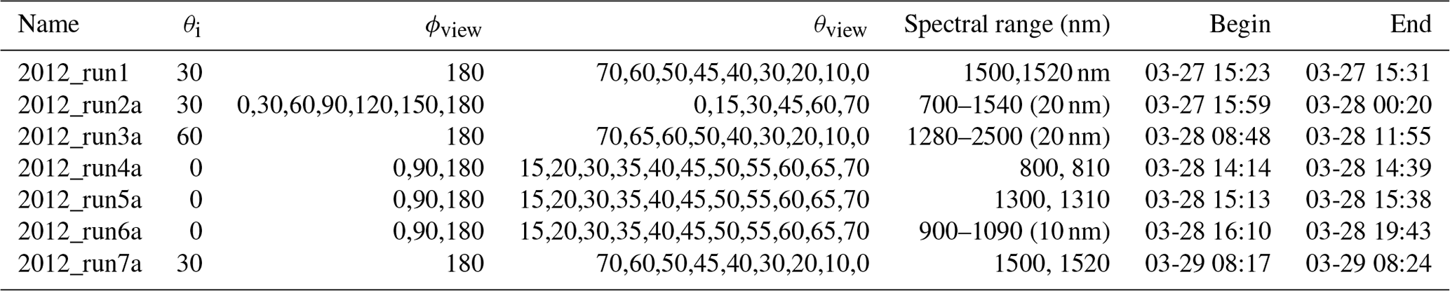
Table A2Geometry and spectral range of S2 optical measurements.
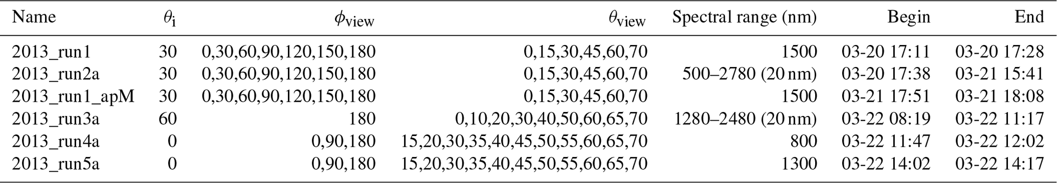
Table A3Geometry and spectral range of S3 optical measurements.


Figure B1Measured (first line) and simulated (second line) reflectances for the three samples (three columns) at 800 nm. The incident zenith angle is 30∘. On the polar plot, the polar angle represents the azimuth, and the radius is proportional to the viewing angles. The dotted circles represent viewing angles of 30, 60, and 70∘. The two lower lines represent the difference between the simulated and measured reflectance for the exponential and μCT-retrieved CLDs. The images used for the simulations are S1_E_1_7m, S2_B_1_7m, and S3_B_1_7m.

Figure B2Measured (first line) and simulated (second line) reflectances for the three samples (three columns) at 1500 nm. The incident zenith angle is 30∘. On the polar plot, the polar angle represents the azimuth, and the radius is proportional to the viewing angles. The dotted circles represent viewing angles of 30, 60, and 70∘. The two lower lines represent the difference between the simulated and measured reflectance for the exponential and μCT-retrieved CLDs. The images used for the simulations are S1_E_1_7m, S2_B_1_7m, and S3_B_1_7m.
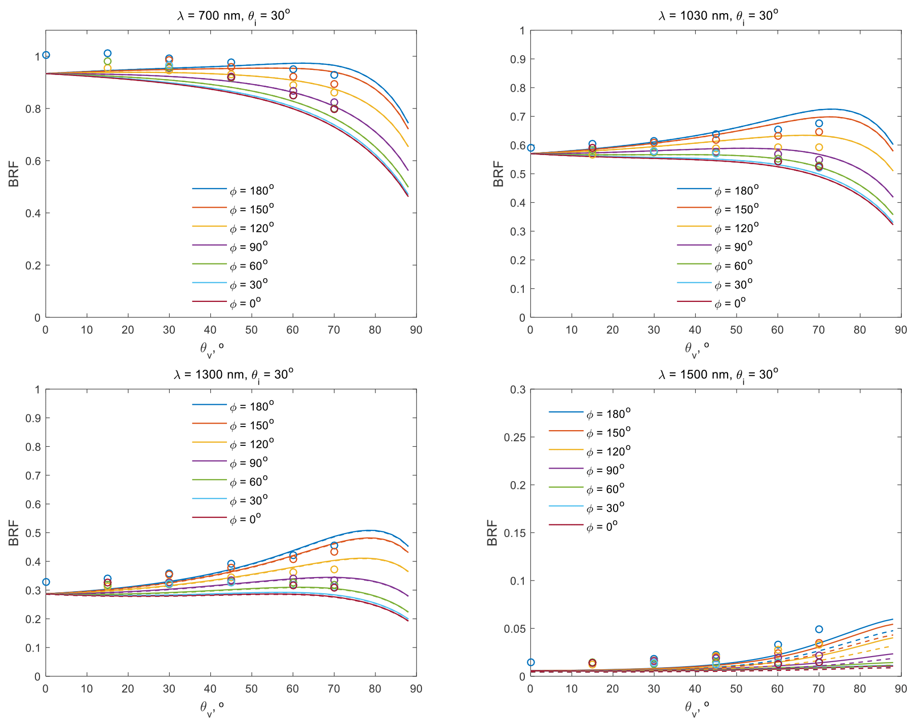
Figure B3BRF measured (circles) and simulated with the exponential (curves) and μCT-retrieved (dashes) CLDs for S1 at 700, 1030, 1300, and 1500 nm. The incident zenith angle is 30∘. The different colours correspond to the azimuth. The μCT-retrieved CLDs are averaged across all of the S2 X-ray images.
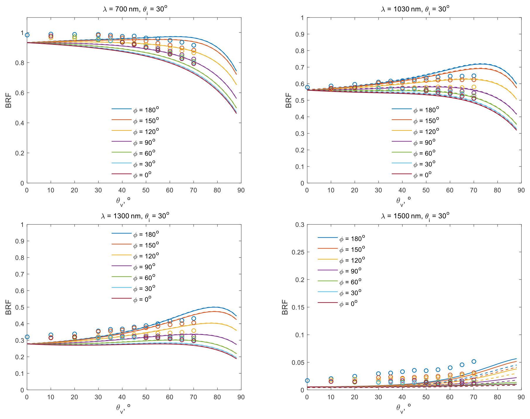
Figure B4BRF measured (circles) and simulated with the exponential (curves) and μCT-retrieved (dashes) CLDs for S1 at 700, 1030, 1300, and 1500 nm. The incident zenith angle is 30∘. The different colours correspond to the azimuth. The μCT-retrieved CLDs are averaged across all of the S3 X-ray images.
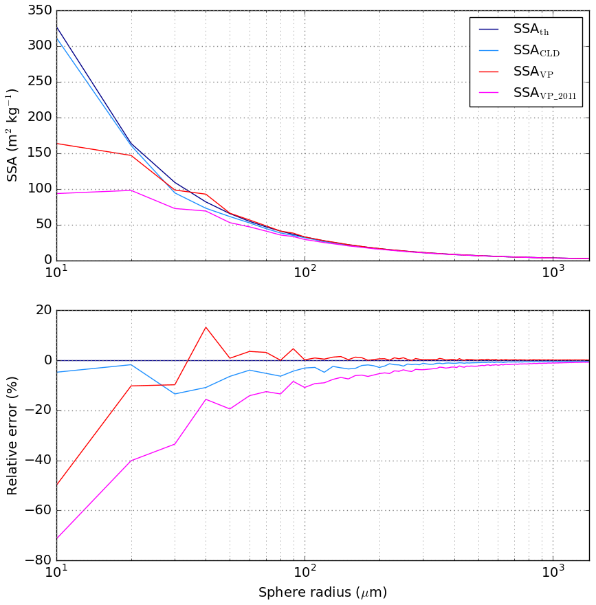
Figure C1SSA estimated from different methods for spheres and their relative error compared to the theoretical value SSAth. SSACLD and SSAVP are defined in Eqs. (6) and (7) respectively. SSAVP_2011 is described in Flin et al. (2011). Sphere radius ranges from R=1 to R=140 voxel (1 voxel was arbitrarily chosen to correspond to 10 µm) – overview in log scale. Note that here, only individual spheres (perfectly isotropic objects) are considered, which favours the SSACLD estimation.
Table D1Manual measurements of density. The heights of the upper and lower boundaries of the sample used for density measurements are indicated in the table.
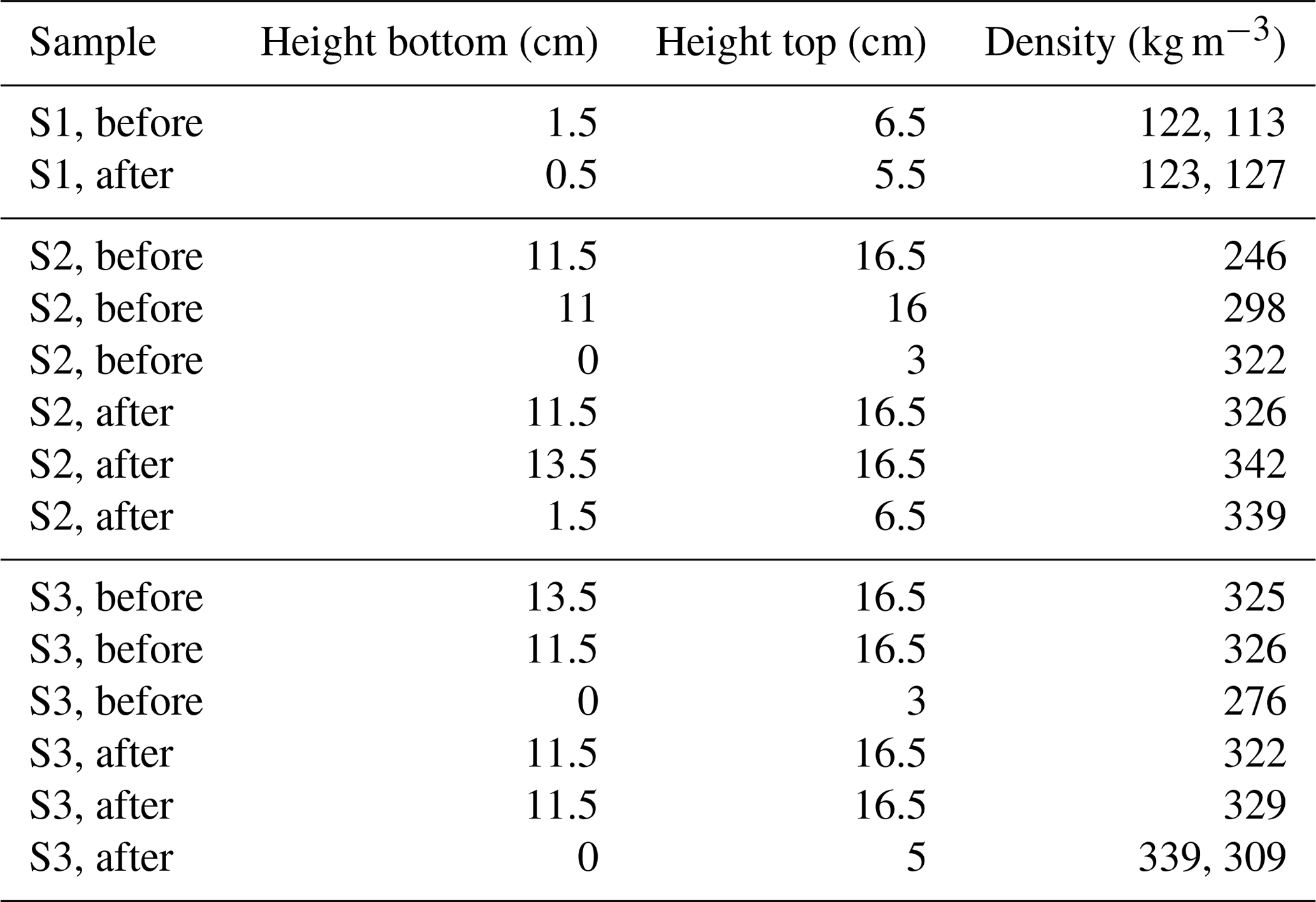
Table D2Manual measurements of SSA. The heights of the upper and lower boundaries of the sample used for SSA measurements are indicated in the table.
The BRF dataset is available in the PANGAEA database along with the CLDs and the simulation results at https://doi.pangaea.de/10.1594/PANGAEA.935028 (Dumont et al., 2021). All simulations are based on the equations from Malinka (2014) and Malinka et al. (2016). Other numerical data used in the study are available directly in the tables, in the main text or in the appendices.
MD led and wrote the study. FF conducted the X-ray tomography measurements and the 3D image analysis. AM performed the analysis of the CLDs and their links to the snow reflectance and made the appropriate simulations. OB conducted the BRF measurements together with MD. PH and PL performed the 3D image processing. BL, AD, and NC prepared the snow samples with the two first authors and contributed to the X-ray tomography measurements. SRdR and EA contributed to the X-ray tomography measurements.
The authors declare that they have no conflict of interest.
Publisher’s note: Copernicus Publications remains neutral with regard to jurisdictional claims in published maps and institutional affiliations.
CNRM/CEN is part of Labex OSUG@2020 (ANR-10-LABX-0056). The 3SR lab is part of the LabEx Tec 21 (Investissements d’Avenir, grant agreement ANR-11-LABX-0030). The authors are thankful to Quentin Libois, Ghislain Picard, Henning Löwe, and Quirine Krol for fruitful discussions on the paper. Pascal Charrier, Jacques Roulle, Philippe Puglièse, and Laurent Pézard are also thanked for their help in the experimental part of the study. The authors further thank the two anonymous reviewers for the helpful comments on the manuscript.
This work was funded by ANR grants DigitalSnow (ANR-11-BS02-009), EBONI (ANR-16-CE01-0006), and MiMESis-3D (ANR-19-CE01-0009); the State Research Program “Photonics, Opto- and Microelectronics'; and the National Academy of Sciences of Belarus. Marie Dumont has received funding from the European Research Council (ERC) under the European Union’s Horizon 2020 research and innovation programme (grant agreement no. 949516, IVORI).
This paper was edited by Kaitlin Keegan and reviewed by two anonymous referees.
Arnaud, L., Picard, G., Champollion, N., Domine, F., Gallet, J.-C., Lefebvre, E., Fily, M., and Barnola, J.-M.: Measurement of vertical profiles of snow specific surface area with a 1 cm resolution using infrared reflectance: instrument description and validation, J. Glaciol., 57, 17–29, https://doi.org/10.3189/002214311795306664, 2011. a, b
Bond, T. C. and Bergstrom, R. W.: Light Absorption by Carbonaceous Particles: An Investigative Review, Aerosol Sci. Technol., 40, 27–67, https://doi.org/10.1080/02786820500421521, 2006. a
Bonnefoy, N.: Développement d'un spectrophoto-goniomètre pour l'étude de la réflectance bidirectionnelle de surfaces géophysiques: application au soufre et perspectives pour le satellite Io, PhD thesis, Université Joseph Fourier, Grenoble, 2001. a
Brissaud, O., Schmitt, B., Bonnefoy, N., Doute, S., Rabou, P., Grundy, W., and Fily, M.: Spectrogonio radiometer for the study of the bidirectional reflectance and polarization functions of planetary surfaces. 1. Design and tests, Appl. Opt., 43, 1926–1937, 2004. a, b
Brzoska, J.-B., Flin, F., and Barckicke, J.: Explicit iterative computation of diffusive vapour field in the 3-D snow matrix: preliminary results for low flux metamorphism, Ann. Glaciol., 48, 13–18, https://doi.org/10.3189/172756408784700798, 2008. a
Calonne, N., Flin, F., Morin, S., Lesaffre, B., du Roscoat, S. R., and Geindreau, C.: Numerical and experimental investigations of the effective thermal conductivity of snow, Geophys. Res. Lett., 38, L23501, https://doi.org/10.1029/2011GL049234, 2011. a
Calonne, N., Geindreau, C., Flin, F., Morin, S., Lesaffre, B., Rolland du Roscoat, S., and Charrier, P.: 3-D image-based numerical computations of snow permeability: links to specific surface area, density, and microstructural anisotropy, The Cryosphere, 6, 939–951, https://doi.org/10.5194/tc-6-939-2012, 2012. a, b
Calonne, N., Flin, F., Geindreau, C., Lesaffre, B., and Rolland du Roscoat, S.: Study of a temperature gradient metamorphism of snow from 3-D images: time evolution of microstructures, physical properties and their associated anisotropy, The Cryosphere, 8, 2255–2274, https://doi.org/10.5194/tc-8-2255-2014, 2014a. a, b, c, d, e
Calonne, N., Geindreau, C., and Flin, F.: Macroscopic modeling for heat and water vapor transfer in dry snow by homogenization, J. Phys. Chem. B, 118, 13393–13403, https://doi.org/10.1021/jp5052535, 2014b. a, b
Carlsen, T., Birnbaum, G., Ehrlich, A., Helm, V., Jäkel, E., Schäfer, M., and Wendisch, M.: Parameterizing anisotropic reflectance of snow surfaces from airborne digital camera observations in Antarctica, The Cryosphere, 14, 3959–3978, https://doi.org/10.5194/tc-14-3959-2020, 2020. a
Carmagnola, C. M., Domine, F., Dumont, M., Wright, P., Strellis, B., Bergin, M., Dibb, J., Picard, G., Libois, Q., Arnaud, L., and Morin, S.: Snow spectral albedo at Summit, Greenland: measurements and numerical simulations based on physical and chemical properties of the snowpack, The Cryosphere, 7, 1139–1160, https://doi.org/10.5194/tc-7-1139-2013, 2013. a
Carmagnola, C. M., Morin, S., Lafaysse, M., Domine, F., Lesaffre, B., Lejeune, Y., Picard, G., and Arnaud, L.: Implementation and evaluation of prognostic representations of the optical diameter of snow in the SURFEX/ISBA-Crocus detailed snowpack model, The Cryosphere, 8, 417–437, https://doi.org/10.5194/tc-8-417-2014, 2014. a
Dang, C., Fu, Q., and Warren, S. G.: Effect of snow grain shape on snow albedo, J. Atmos. Sci., 73, 3573–3583, 2016. a
Domine, F., Salvatori, R., Legagneux, L., Salzano, R., Fily, M., and Casacchia, R.: Correlation between the specific surface area and the short wave infrared (SWIR) reflectance of snow: preliminary investigation., Cold Reg. Sci. Technol., 46, 60–68, https://doi.org/10.1016/j.coldregions.2006.06.002, 2006. a
Dumont, M., Brissaud, O., Picard, G., Schmitt, B., Gallet, J.-C., and Arnaud, Y.: High-accuracy measurements of snow Bidirectional Reflectance Distribution Function at visible and NIR wavelengths – comparison with modelling results, Atmos. Chem. Phys., 10, 2507–2520, https://doi.org/10.5194/acp-10-2507-2010, 2010. a, b, c, d, e, f
Dumont, M., Flin, F., Malinka, A., Brissaud, O., Hagenmuller, P., Lapalus, P., Calonne, N., Dufour, A., Ando, E., Rolland du Roscoat, S.: Experimental and model-based investigation of the links between snow bidirectional reflectance and snow microstructure, PANGAEA, https://doi.pangaea.de/10.1594/PANGAEA.935028, 2021. a
Fierz, C., Armstrong, R. L., Durand, Y., Etchevers, P., Greene, E., McClung, D. M., Nishimura, K., Satyawali, P. K., and Sokratov, S. A.: The international classification for seasonal snow on the ground, IHP-VII Technical Documents in Hydrology no. 83, IACS Contribution no. 1, available at: http://unesdoc.unesco.org/images/0018/001864/186462e.pdf (last access: 16 August 2021), 2009. a, b, c
Flanner, M. G., Liu, X., Zhou, C., Penner, J. E., and Jiao, C.: Enhanced solar energy absorption by internally-mixed black carbon in snow grains, Atmos. Chem. Phys., 12, 4699–4721, https://doi.org/10.5194/acp-12-4699-2012, 2012. a, b
Flin, F. and Brzoska, J.-B.: The temperature-gradient metamorphism of snow: vapour diffusion model and application to tomographic images, Ann. Glaciol., 49, 17–21, https://doi.org/10.3189/172756408787814834, 2008. a
Flin, F., Brzoska, J.-B., Lesaffre, B., Coléou, C., and Pieritz, R. A.: Full three-dimensional modelling of curvature-dependent snow metamorphism: first results and comparison with experimental tomographic data, J. Phys. D, 36, A49–A54, https://doi.org/10.1088/0022-3727/36/10A/310, 2003. a, b, c, d
Flin, F., Brzoska, J.-B., Lesaffre, B., Coléou, C., and Pieritz, R. A.: Three-dimensional geometric measurements of snow microstructural evolution under isothermal conditions, Ann. Glaciol., 38, 39–44, https://doi.org/10.3189/172756404781814942, 2004. a, b, c
Flin, F., Brzoska, J.-B., Coeurjolly, D., Pieritz, R. A., Lesaffre, B., Coléou, C., Lamboley, P., Teytaud, O., Vignoles, G. L., and Delesse, J.-F.: Adaptive estimation of normals and surface area for discrete 3-D objects: application to snow binary data from X-ray tomography, I.E.E.E. Trans. Image. Process., 14, 585–596, https://doi.org/10.1109/TIP.2005.846021, 2005. a, b
Flin, F., Lesaffre, B., Dufour, A., Gillibert, L., Hasan, A., Rolland du Roscoat, S., Cabanes, S., and Pugliese, P.: On the Computations of Specific Surface Area and Specific Grain Contact Area from Snow 3D Images, edited by: Furukawa, Y., Hokkaido University Press, Sapporo, JP, proceedings of the 12th International Conference on the Physics and Chemistry of Ice held at Sapporo, Japan, 5–10 September 2010, 321–328, 2011. a, b
Gallet, J.-C., Domine, F., Zender, C. S., and Picard, G.: Measurement of the specific surface area of snow using infrared reflectance in an integrating sphere at 1310 and 1550 nm, The Cryosphere, 3, 167–182, https://doi.org/10.5194/tc-3-167-2009, 2009. a, b, c
Grenfell, T. and Warren, S.: Representation of a nonspherical ice particle by a collection of independent spheres for scattering and absorption of radiation, J. Geophys. Res., 104, 31697–31709, https://doi.org/10.1029/2000JC000414, 1999. a
Grundy, W. and Schmitt, B.: The temperature-dependent near-infrared absorption spectrum of hexagonal H(2)O ice, J. Geophys. Res., 103, 25809–25822, https://doi.org/10.1029/98JE00738, 1998. a, b, c, d, e, f, g
Hadley, O. and Kirchstetter, T.: Black-carbon reduction of snow albedo, Nat. Clim. Change, 2, 437–440, https://doi.org/10.1038/nclimate1433, 2012. a
Hagenmuller, P., Chambon, G., Lesaffre, B., Flin, F., and Naaim, M.: Energy-based binary segmentation of snow microtomographic images, J. Glaciol., 59, 859–873, https://doi.org/10.3189/2013JoG13J035, 2013. a, b, c, d
Haussener, S., Gergely, M., Schneebeli, M., and Steinfeld, A.: Determination of the macroscopic optical properties of snow based on exact morphology and direct pore-level heat transfer modeling, J. Geophys. Res.-Earth Surf., 117, F03009, https://doi.org/10.1029/2012JF002332, 2012. a
He, C., Flanner, M. G., Chen, F., Barlage, M., Liou, K.-N., Kang, S., Ming, J., and Qian, Y.: Black carbon-induced snow albedo reduction over the Tibetan Plateau: uncertainties from snow grain shape and aerosol–snow mixing state based on an updated SNICAR model, Atmos. Chem. Phys., 18, 11507–11527, https://doi.org/10.5194/acp-18-11507-2018, 2018. a
Horton, S. and Jamieson, B.: Spectral measurements of surface hoar crystals, J. Glaciol., 63, 477–486, 2017. a
Hudson, S. R., Warren, S. G., Brandt, R. E., Grenfell, T. C., and Six, D.: Spectral bidirectional reflectance of Antarctic snow: Measurements and parameterization, J. Geophys. Res.-Atmos., 111, D18106, https://doi.org/10.1029/2006JD007290, 2006. a, b
Ishimoto, H., Adachi, S., Yamaguchi, S., Tanikawa, T., Aoki, T., and Masuda, K.: Snow particles extracted from X-ray computed microtomography imagery and their single-scattering properties, J. Quant. Spectrosc. Ra., 209, 113–128, 2018. a
Jin, Z., Charlock, T. P., Yang, P., Xie, Y., and Miller, W.: Snow optical properties for different particle shapes with application to snow grain size retrieval and MODIS/CERES radiance comparison over Antarctica, Remote Sens. Environ., 112, 3563–3581, https://doi.org/10.1016/j.rse.2008.04.011, 2008. a
Kaempfer, T. U., Hopkins, M. A., and Perovich, D. K.: A three-dimensional microstructure-based photon-tracking model of radiative transfer in snow, J. Geophys. Res.-Atmos., 112, D24113, https://doi.org/10.1029/2006JD008239, 2007. a, b
Kokhanovsky, A. and Zege, E.: Scattering optics of snow, Appl. Opt., 43, 1589–1602, https://doi.org/10.1364/AO.43.001589, 2004. a, b
Kou, L., Labrie, D., and Chylek, P.: Refractive indeces of water and ice in the 0.65 microns to 2.5 microns spectral range, Appl. Opt., 32, 3531–3540, 1993. a, b, c, d
Krol, Q. and Löwe, H.: Relating optical and microwave grain metrics of snow: the relevance of grain shape, The Cryosphere, 10, 2847–2863, https://doi.org/10.5194/tc-10-2847-2016, 2016a. a, b, c, d, e, f
Krol, Q. and Löwe, H.: Analysis of local ice crystal growth in snow, J. Glaciol., 62, 378–390, https://doi.org/10.1017/jog.2016.32, 2016b. a
Libois, Q., Picard, G., France, J. L., Arnaud, L., Dumont, M., Carmagnola, C. M., and King, M. D.: Influence of grain shape on light penetration in snow, The Cryosphere, 7, 1803–1818, https://doi.org/10.5194/tc-7-1803-2013, 2013. a, b
Libois, Q., Picard, G., Arnaud, L., Morin, S., and Brun, E.: Modeling the impact of snow drift on the decameter-scale variability of snow properties on the Antarctic Plateau, J. Geophys. Res., 119, 11662–11681, https://doi.org/10.1002/2014JD022361, 2014. a
Libois, Q., Picard, G., Arnaud, L., Dumont, M., Lafaysse, M., Morin, S., and Lefebvre, E.: Summertime evolution of snow specific surface area close to the surface on the Antarctic Plateau, The Cryosphere, 9, 2383–2398, https://doi.org/10.5194/tc-9-2383-2015, 2015. a
Liou, K., Takano, Y., and Yang, P.: Light absorption and scattering by aggregates: Application to black carbon and snow grains, J. Quant. Spectrosc. Ra., 112, 1581–1594, 2011. a
Löwe, H., Riche, F., and Schneebeli, M.: A general treatment of snow microstructure exemplified by an improved relation for thermal conductivity, The Cryosphere, 7, 1473–1480, https://doi.org/10.5194/tc-7-1473-2013, 2013. a, b
Malinka, A., Zege, E., Heygster, G., and Istomina, L.: Reflective properties of white sea ice and snow, The Cryosphere, 10, 2541–2557, https://doi.org/10.5194/tc-10-2541-2016, 2016. a, b, c, d, e, f, g, h
Malinka, A. V.: Light scattering in porous materials: Geometrical optics and stereological approach, J. Quant. Spectrosc. Ra., 141, 14–23, https://doi.org/10.1016/j.jqsrt.2014.02.022, 2014. a, b, c, d, e, f, g, h, i, j, k
Mary, A., Dumont, M., Dedieu, J.-P., Durand, Y., Sirguey, P., Milhem, H., Mestre, O., Negi, H. S., Kokhanovsky, A. A., Lafaysse, M., and Morin, S.: Intercomparison of retrieval algorithms for the specific surface area of snow from near-infrared satellite data in mountainous terrain, and comparison with the output of a semi-distributed snowpack model, The Cryosphere, 7, 741–761, https://doi.org/10.5194/tc-7-741-2013, 2013. a
Painter, T. H. and Dozier, J.: Measurements of the hemispherical-directional reflectance of snow at fine spectral and angular resolution, J. Geophys. Res.-Atmos., 109, D18115, https://doi.org/10.1029/2003JD004458, 2004. a
Petrasch, J., Wyss, P., and Steinfeld, A.: Tomography-based Monte Carlo determination of radiative properties of reticulate porous ceramics, J. Quant. Spectrosc. Ra., 105, 180–197, 2007. a
Picard, G., Brucker, L., Fily, M., Gallée, H., and Krinner, G.: Modeling time series of microwave brightness temperature in Antarctica, J. Glaciol., 55, 537–551, 2009. a, b
Proksch, M., Rutter, N., Fierz, C., and Schneebeli, M.: Intercomparison of snow density measurements: bias, precision, and vertical resolution, The Cryosphere, 10, 371–384, https://doi.org/10.5194/tc-10-371-2016, 2016. a
Räisänen, P., Kokhanovsky, A., Guyot, G., Jourdan, O., and Nousiainen, T.: Parameterization of single-scattering properties of snow, The Cryosphere, 9, 1277–1301, https://doi.org/10.5194/tc-9-1277-2015, 2015. a
Schaepman-Strub, G., Schaepman, M., Painter, T. H., Dangel, S., and Martonchik, J.: Reflectance quantities in optical remote sensing – definitions and case studies, Remote Sens. Environ., 103, 27–42, https://doi.org/10.1016/j.rse.2006.03.002, 2006. a
Schleef, S., Löwe, H., and Schneebeli, M.: Influence of stress, temperature and crystal morphology on isothermal densification and specific surface area decrease of new snow, The Cryosphere, 8, 1825–1838, https://doi.org/10.5194/tc-8-1825-2014, 2014. a
Srivastava, P. K., Chandel, C., Mahajan, P., and Pankaj, P.: Prediction of anisotropic elastic properties of snow from its microstructure, Cold Reg. Sci. Technol., 125, 85–100, https://doi.org/10.1016/j.coldregions.2016.02.002, 2016. a
Stanton, B., Miller, D., Adams, E., and Shaw, J. A.: Bidirectional-reflectance measurements for various snow crystal morphologies, Cold Reg. Sci. Technol., 124, 110–117, 2016. a, b, c, d
Torquato, S.: Random Heterogeneous Materials: Microstructure and Macroscopic Properties, Springer-Verlag, New York, 2002. a, b
Tuzet, F., Dumont, M., Arnaud, L., Voisin, D., Lamare, M., Larue, F., Revuelto, J., and Picard, G.: Influence of light-absorbing particles on snow spectral irradiance profiles, The Cryosphere, 13, 2169–2187, https://doi.org/10.5194/tc-13-2169-2019, 2019. a
Tuzet, F., Dumont, M., Picard, G., Lamare, M., Voisin, D., Nabat, P., Lafaysse, M., Larue, F., Revuelto, J., and Arnaud, L.: Quantification of the radiative impact of light-absorbing particles during two contrasted snow seasons at Col du Lautaret (2058 m a.s.l., French Alps), The Cryosphere, 14, 4553–4579, https://doi.org/10.5194/tc-14-4553-2020, 2020. a
Varsa, P. M., Baranoski, G. V., and Kimmel, B. W.: SPLITSnow: A spectral light transport model for snow, Remote Sens. Environ., 255, 112272, https://doi.org/10.1016/j.rse.2020.112272, 2021. a
Warren, S.: Optical properties of snow, Rev. Geophys., 20, 67–89, https://doi.org/10.1029/RG020i001p00067, 1982. a, b
Warren, S. and Brandt, R.: Optical constants of ice from the ultraviolet to the microwave: A revised compilation, J. Geophys. Res., 113, D14220, https://doi.org/10.1029/2007JD009744, 2008. a, b, c, d, e
Warren, S. G.: Optical contants of ice from the ultraviolet to the microwave, Appl. Opt., 23, 1206–1225, 1984. a, b
Warren, S. G., Brandt, R. E., and O'Rawe Hinton, P.: Effect of surface roughness on bidirectional reflectance of Antarctic snow, J. Geophys. Res.-Planets, 103, 25789–25807, https://doi.org/10.1029/98JE01898, 1998. a
Wautier, A., Geindreau, C., and Flin, F.: Linking snow microstructure to its macroscopic elastic stiffness tensor: A numerical homogenization method and its application to 3-D images from X-ray tomography, Geophys. Res. Lett., 42, 8031–8041, https://doi.org/10.1002/2015GL065227, 2015. a
Wautier, A., Geindreau, C., and Flin, F.: Numerical homogenization of the viscoplastic behavior of snow based on X-ray tomography images, The Cryosphere, 11, 1465–1485, https://doi.org/10.5194/tc-11-1465-2017, 2017. a
Xie, Y., Yang, P., Gao, B.-C., Kattawar, G. W., and Mishchenko, M. I.: Effect of ice crystal shape and effective size on snow bidirectional reflectance, J. Quant. Spectrosc. Ra., 100, 457–469, 2006. a, b
- Abstract
- Introduction
- Materials and methods
- Results
- Discussions and conclusions
- Appendix A: Overview of the optical measurements
- Appendix B: Model vs. measurements
- Appendix C: Evaluation of SSA on calibrated spheres using different methods
- Appendix D: Density and SSA manual measurements
- Code and data availability
- Author contributions
- Competing interests
- Disclaimer
- Acknowledgements
- Financial support
- Review statement
- References