Snow depth time series retrieval by time-lapse photography: Finnish and Italian case studies

The capability of time-lapse photography to retrieve snow depth time series was tested. Historically, snow depth has been measured manually by rulers, with a temporal resolution of once per day, and it is a time-consuming activity. In the last few decades, ultrasonic and/or optical sensors have been developed to obtain automatic and regular measurements with higher temporal resolution and accuracy. The Finnish Meteorological Institute Image Processing Toolbox (FMIPROT) has been used to retrieve the snow depth time series from camera images of a snow stake on the ground by implementing an algorithm based on the brightness difference and contour detection. Three case studies have been illustrated to highlight potentialities and pitfalls of time-lapse photography in retrieving the snow depth time series: Sodankylä peatland, a boreal forested site in Finland, and Gressoney-La-Trinité Dejola and Careser Dam, two alpine sites in Italy. This study presents new possibilities and advantages in the retrieval of snow depth in general and snow depth time series specifically, which can be summarized as follows: (1) high temporal resolution – hourly or sub-hourly time series, depending on the camera's scan rate; (2) high accuracy levels – comparable to the most common method (manual measurements); (3) reliability and visual identification of errors or misclassifications; (4) low-cost solution; and (5) remote sensing technique – can be easily extended in remote and dangerous areas.

The proper geometrical configuration between camera and stake, highlighting the main characteristics which each single component must have, has been proposed. Root mean square errors (RMSEs) and Nash–Sutcliffe efficiencies (NSEs) were calculated for all three case studies comparing with estimates from both the FMIPROT and visual inspection of images directly. The NSE values were 0.917, 0.963 and 0.916, while RMSEs were 0.039, 0.052 and 0.108 m for Sodankylä, Gressoney and Careser, respectively. In terms of accuracy, the Sodankylä case study gave better results. The worst performances occurred at Careser Dam located at 2600 m a.s.l., where extreme weather conditions and a low temporal resolution of the camera occur, strongly affecting the clarity of the images.

1 Introduction

Seasonal snow has an important role in the Earth's climate system and a strong influence on its energy balance (Henderson et al., 2018), as well as providing a fundamental contribution to the river discharge in catchments located in alpine and cold regions (Mastrotheodoros et al., 2020). Due to the inhomogeneous spatial distribution of snow, traditional in situ measurement techniques can hardly provide exhaustive information about snow variability (Lundberg et al., 2010). Remote sensing is becoming the most widespread technique to evaluate snow cover (Da Ronco et al., 2020), snow depth (De Michele et al., 2016; Avanzi et al., 2018; Lievens et al., 2019) and snow water equivalent (Takala et al., 2011, 2017).

From a hydrological point of view, the main variable of snowpack is the snow water equivalent (SWE), rather than snow depth (SD), or snow density (ρ_s) (De Michele et al., 2013; Avanzi et al., 2015, 2014). The snow water equivalent is a function of snow depth and snow density (DeWalle and Rango, 2008) given in Eq. (1) below:

$$\begin{array}{}\text{(1)}& \text{SWE}\left(t\right)=\text{SD}\left(t\right){\displaystyle \frac{{\mathit{\rho }}_{\mathrm{s}}\left(t\right)}{{\mathit{\rho }}_{\mathrm{w}}}},\end{array}$$

where ρ_w is the density of water.

The depth is the simplest characteristic of snowpack, which can be easily detected with manual measurements within field campaigns (snow courses) (Pirazzini et al., 2018). This is particularly true in Alpine regions, especially related to hydropower production and near dam sites, where manual measurements by rulers or snowboards (pieces of plywood, painted white, that act as a surface to collect snow, typically 0.4×0.4 m or 0.4×0.6 m) have generally been programmed to monitor snow processes during the accumulation and melting seasons. Uncertainties related to snow depth measurements depend on the temporal and spatial resolution of the measurement methods. Manual measurements by rulers generally have a daily resolution with 2–3 cm accuracy. Ultrasonic sensor measurements have a finer temporal resolution (1 h or less) with 1 mm accuracy. Satellite measurements are useful for estimating snow depth in a wide region with less accuracy (10 cm) and a coarse temporal resolution (depending on orbit period).

Time-lapse photography has been used in the literature to retrieve some characteristics of the snow such as snow depth, snow canopy interception, snow settling, fractional snow cover on the ground, albedo and state of precipitation. Mainly applications have been in remote areas, Greenland or the Arctic region, or in mountain regions and related to the snow accumulation on glacierized areas (Christiansen, 2001; Floyd and Weiler, 2008; Farinotti et al., 2010; Parajka et al., 2012; Bernard et al., 2013; Garvelmann et al., 2013; Hedrick and Marshall, 2014; Dong and Menzel, 2017).

Starting from 2001, continuous automatic digital photography has been tested in high-Arctic Greenland to monitor snow cover conditions in remote areas by Christiansen (2001). Daily photographs covered a 100 m transect through a seasonal snow patch and thus on an annual basis also yielded information on snow cover duration in the different vegetation zones of the snow patch. Photographs, combined with measurements taken by automatic weather stations, allowed for studying wind-induced snow redistribution in different thin snow-covered areas. Christiansen (2001) suggested that this method can be seen as a valid alternative to the traditional snow monitoring methods by providing areal information and not only point measurements. Floyd and Weiler (2008) designed an automatic time-lapse photography network to monitor the state of precipitation (rain vs. snow), snow accumulation and ablation, canopy interception, and unloading of snow from the canopy; they also defined image analysis software which can calculate snow parameters from images.

Farinotti et al. (2010) tried to use conventional oblique photography combined with a temperature index melt and accumulation model to infer the snow accumulation distribution of a small Alpine catchment.

Parajka et al. (2012) studied the potential of time-lapse photography to retrieve snow cover for hydrological purposes at a small catchment scale. They designed and tested a monitoring system, which allowed for multi-resolution observations of snow cover characteristics. They carried out investigations about snow cover, snow depth and snowfall interception, both in the area near the camera and in a wider range. They tested the multi-resolution design at three sites in the eastern part of the Austrian Alps, using photographs at hourly time steps, showing that it is possible to process a large number of photos by using an automatic procedure for accurate snow depth readings. Using five stakes, it is possible to cross-check snow depth estimations, omitting the largest and smallest readings and obtaining a robust estimate of the snow depth. The snow depth algorithm retrieval was not described in detail, but the routine calculated the visible markers from the top of the stake and then estimated the snow depth as a difference from the whole stake length. The accuracy was not very high because the snow stake had 10 cm markers and the camera had only a 3-megapixel resolution. Some kind of sensor or manual measurements were used to compare the accuracy.

Bernard et al. (2013) installed, around the Austre Lovénbreen glacier basin (Norway, 79^∘ N), automated digital cameras in the context of long-term monitoring of snow and ice dynamics with a high temporal and spatial resolution. Moreover, six camera stations were oriented to observe 96 % of the glacierized area, monitoring in the hydrological year 2009 the snow cover evolution and studying the accumulation due to snowfall events and the ablation caused by precipitation or warm temperature.

Garvelmann et al. (2013) defined a camera network to quantify snow processes such as snow depth, snow canopy interception, albedo and the state of precipitation. Regarding snow depth retrieval, they developed a semi-automatic approach, using images in which snow stakes with 10 cm red and black markers were visible. The main limitation was that they needed to define the number of pixels of a 10 cm bar of the stake and of the whole stake length with a procedure of cursor clicks which made it time-consuming. In addition, the accuracy was limited by the 10 cm snow stake markers, and the comparison was made only against visual observations. They reported an accuracy of 7.1 cm within the period of December 2011 to April 2012.

Hedrick and Marshall (2014), within a test site, defined an automated, low-cost and safe snow depth retrieval system in avalanche terrain using time-lapse photography; however, no accuracy parameter was reported, providing only a visual comparison.

Dong and Menzel (2017) focused on snow process monitoring in mountain forests with time-lapse photography. They developed a semi-automatic procedure to retrieve the snow depth from digital images, which exhibited high consistency with manual measurements and station-based recordings.

In conclusion, some works about snow depth retrieval from time-lapse photography are available, but presently, there is no fully automatic procedure to retrieve snow depth in real time from the snow stake images and thus generate time series. Additionally, there are no extensive studies about the accuracy of snow depth retrieval from time-lapse photography.

In this study, we present an automated procedure with defined region-of-interest (ROI) inputs to retrieve snow depth in real time and snow depth time series from time-lapse photography. The automated procedure is based on an algorithm implemented within the Finnish Meteorological Institute Image Processing Toolbox (FMIPROT), which uses the brightness difference between the snowpack and the stake's markers in digital images. Retrieval of snow depth time series for more than one hydrological year is presented. The procedure was tested in three different sites, one in the boreal forest in the Arctic region and two in the Italian Alps. In the last two sites, existing configurations of camera and stake were not set up for retrieving snow depth specifically. That is why the proper geometric and parameter configurations of the camera–stake system, the sources of errors, and post-processing procedure corrections were also investigated. Moreover, the following results will be shown:

• -

  how the accuracy of snow depth estimations can be increased using stakes with 1 cm spacing markers,

• -

  proper geometric and parameter configurations of the camera–stake system,

• -

  sources of errors and post-processing procedure corrections.

The proposed automated procedure can be taken as a reference for (a) validating existing methods of snow depth retrieval, (b) comparing results in terms of amount and precipitation classification, and (c) defining an alternative method to monitor dynamics of snowpack with a high temporal resolution. The paper is organized into the following sections: in Sect. 2 the method and algorithm are illustrated; in Sect. 3 the case studies are described; in Sect. 4 results are given; in Sect. 5 a discussion of results is provided; in Sect. 6 conclusions are drawn.

2 Method

In this section it is described how camera images (which show a snow stake with graduated markers) can be used to retrieve the snow depth. We introduce the FMIPROT; then we explain the automated procedure on the retrieval of snow depth, and finally we present a correction method to obtain a more affordable snow depth time series.

The FMIPROT (Tanis et al., 2018) was developed for analyzing digital images from multiple camera networks for various applications such as vegetation phenology and monitoring of snow cover. This toolbox has a user-friendly graphical user interface (GUI) and can be used easily with only basic computing knowledge. The interface allows one to easily download and/or read images from camera networks (online or offline) which provide continuous series with the aim to monitor some environmental features such as phenology and snow.

Current features are automatic image downloading and handling; GUI-based selection of a region of interest (ROI); an automatic analysis chain; GUI-based plotting; the creation of HTML reports with results shown on interactive plots; ROI-based indices such as the green fraction index (GF), red fraction index (RF), blue fraction index (BF), green–red vegetation index (GRVI) and green excess index (GEI); snow cover fraction estimation with geo-rectification; snow depth estimation; and time-lapse animation. The FMIPROT is freely available at the website https://fmiprot.fmi.fi (last access: 13 January 2021). In the next section, the automated procedure is described for the snow depth retrieval developed from the protocol.

2.1 Retrieval procedure of snow depth

The automated procedure for the retrieval of snow depth is given in Fig. 1. The retrieval procedure of snow depth is articulated in eight steps:

• 1.

  ROI identification. Starting from an image without snow cover, the region of interest is selected with the FMIPROT by drawing a polygon, which defines a quadrilateral around the snow stake. So, the pixel-counting algorithm clips each image considering only pixels inside of this. In addition, the real length of the whole ROI must be defined in meters. In most of the cases, it is better to define a polygon which includes the whole stake from the ground to the top level, but it is not mandatory. To avoid snow depth underestimation, the top of the ROI must be greater than the maximum snow height level.

• 2.

  Gaussian filtering. On each image, a Gaussian filter based on the parameter σ can be applied, which smooths the brightness difference, reducing pixel noises.

• 3.

  Thresholding. Comparing the pixel value with a predefined brightness threshold T_S, we can classify each pixel as black or white (0 or 1). This threshold can vary widely, selecting different observation periods, and the best one must be defined to reduce misclassifications. Related to this parameter it is better to have a strong reflectance difference between the stake background and markers. The best coloration of the stake is found to be yellow or white for the background and a dark color (i.e., black) for the markers.

• 4.

  Segmentation. This is the process of partitioning a digital image into multiple segments. In our case this process defines the marker's contour with the edge detection. That is why it is fundamental that the stake must be graduated. In fact, the snow depth estimation resolution depends on the marker spacing. Markers with little distance can improve estimation accuracy, but remaining above 0.01 m is suggested, because they must be identified clearly considering the distance between the stake and camera.

• 5.

  Shape filtering. This consists of characterizing and filtering objects in binary scenes by their shape. Detected shapes that are not similar to squares are filtered out, as they are not the markers but noise.

• 6.

  Marker height. The pixel row for each marker (d_i) is read from the remaining shapes. Note that the counting started from the upper part of the image; 0 means the top of the ROI.

• 7.

  Position of the first visible marker. The snow depth layer is located near the first visible marker from the bottom of the stake, which is characterized by the minimum height value. Its pixel row is defined as

  $$\begin{array}{}\text{(2)}& \text{SD}=min\left(H_i\right)\left[\text{no. of pixels}\right].\end{array}$$
• 8.

  Retrieving snow depth. The number of pixels must be converted into the real depth, multiplying it with the ratio between the real snow stake length (L_s) in meters and the number of pixels of the whole stake (H_S):

  $$\begin{array}{}\text{(3)}& \text{SD}=S_{\mathrm{D}}{\displaystyle \frac{L_{\mathrm{s}}}{H_{\mathrm{S}}}}\left[\mathrm{m}\right].\end{array}$$

  The counting-pixel algorithm routine required the parameters' definition; in particular for each case study the best threshold (T_S) and the Gaussian filter (σ), which allows us to better estimate snow depth, have to be chosen. The best parameter configuration allows us to increase the brightness contrast between the snowpack layer and stake's markers. The threshold can vary widely, because images have different resolutions, due to different geometrical configurations and especially related to the different visibility conditions in terms of brightness and luminance. The same thing happened for the Gaussian filter σ, which can assume values from 1 to 10. Firstly, the algorithm was run in a small period (10 d) to find the best parameters of configuration in order to reproduce the visually estimated snow depth. After having found the best parameters, the algorithm was run for the whole observation period.

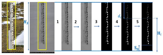
Figure 1 Snow depth retrieval procedure algorithm (SPICE (Solid Precipitation Intercomparison Experiment) site – Sodankylä).

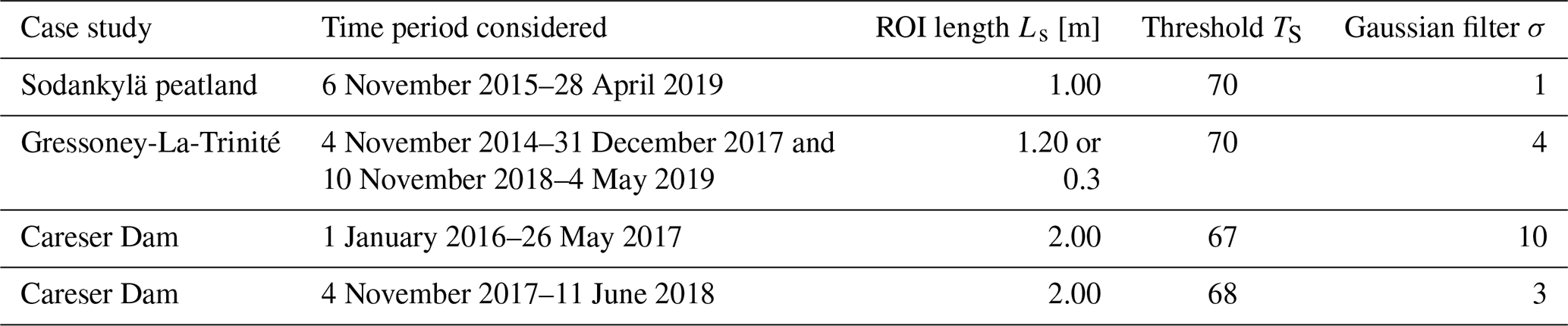
In Table 1, the values of parameters used are reported for each case study. As can be seen, depending on the maximum snow depth observed on the ground, different values of ROI length L_s were used: Careser Dam is located near 2600 m a.s.l., so the expected maximum snow depth is near 2 m; thus L_s=2 m. In contrast at the Sodankylä peatland site, a smaller value equal to 1 m was observed; thus L_s=1 m. The values for the brightness threshold T_s and the Gaussian filter σ were used from 65 to 70 and from 1 to 10, respectively.

Table 1 Snow depth algorithm parameters for each case study.

The best method consists of repeating the run of the algorithm with different parameter combinations and defining an “ensemble” snow depth as the mean of those. This technique improves results by obtaining a more reliable snow depth time series as shown in the Fig. S4 in the Supplement.

Here the principal aim is not only the retrieval of the single snow depth value but also defining a snow depth time series with high accuracy. This issue is very important for hydrological purposes, but until now the application of time-lapse photography has been tested only for small time periods (months). This procedure will be defined without any snow depth measurement knowledge, in other terms, without data assimilation, because in most cases there are only images without real measurements.

The algorithm provides snow depth retrieval close to real values with a high percentage, but sometimes it can fail, especially when atmospheric conditions are bad. In these cases, estimated snow depth values were found to be close to 0 or classified as not a number (NaN) or affected by high biases. A procedure was defined to remove these incorrect values, running the algorithm five times with different parameter combinations. In particular, the brightness threshold parameter T_s=70 was fixed, and five different values of the Gaussian filter parameter σ from 1 to 5 were defined. Then each time series was used to define the “corrected snow depth time series”. Then all the necessary steps were reported to run the retrieval algorithm: at first, the single snow depth time series estimated with fixed threshold T_s and Gaussian filter parameter σ, called SD_O(t), where “O” means original, was loaded. Then errors and high biases were removed to obtain a more correct snow depth time series, which is called SD_C(t).

First of all, with an assumption that it was difficult to have snowfall or melting of much more than 0.02 m in 1 h, the time series was reclassified as a not-a-number SD_O(t) if there was a difference of more than 0.02 m to the previous or the following one. In some cases, it was noticed that a cluster of misclassifications, i.e., values near not a number, were suspicious, so it was decided to reclassify each value near to a not-a-number value as not a number itself. As a summary these conditions can be given below:

$$\begin{array}{}\text{(4)}& {\displaystyle }\begin{array}{rl}\text{if }& (\left|{\text{SD}}_{\mathrm{O}}\left(t\right)-{\text{SD}}_{\mathrm{O}}(t-\mathrm{1})\right|>\mathrm{2}\mathrm{cm}\text{or}\\ & \left|{\text{SD}}_{\mathrm{O}}(t+\mathrm{1})-{\text{SD}}_{\mathrm{O}}\left(t\right)\right|>\mathrm{2}\mathrm{cm}),\text{then}\\ & {\text{SD}}_{\mathrm{C}}\left(t\right)=\text{NaN};\end{array}\text{(5)}& {\displaystyle }\begin{array}{rl}\text{if }& \left({\text{SD}}_{\mathrm{O}}\right(t)=\text{NaN}),\text{then}{\text{SD}}_{\mathrm{C}}(t-\mathrm{1})=\text{NaN and}\\ & {\text{SD}}_{\mathrm{C}}(t+\mathrm{1})=\text{NaN}.\end{array}\end{array}$$

In addition, in order to remove noise due to the optical sensor, the value at time t was corrected if this had an absolute difference of more than 0.005 m (S) from the mean of the 12 (W) following and previous values. That is why the value at time t was substituted with a moving average of 24 values centered at time t. If there were NaN values inside this window, they were not considered:

$$\begin{array}{}\text{(6)}& \begin{array}{rl}\text{if}& (\left|{\text{SD}}_{\mathrm{C}}\left(t\right)-{\displaystyle \frac{\mathrm{1}}{n}}\sum _{t-W}^t{\text{SD}}_{\mathrm{C}}\left(t\right)\right|>S\text{and}\\ & \left|{\text{SD}}_{\mathrm{C}}\left(t\right)\right.-\left.{\displaystyle \frac{\mathrm{1}}{n}}\sum _t^{t+W}{\text{SD}}_{\mathrm{C}}\left(t\right)\right|>S),\\ & \text{then}{\text{SD}}_{\mathrm{C}}\left(t\right)={\displaystyle \frac{\mathrm{1}}{n}}\sum _{t-W}^{t+W}{\text{SD}}_{\mathrm{C}}\left(t\right),\end{array}\end{array}$$

where S is the maximum snow depth difference, equal to 0.005 m, and W is the window length of the moving average procedure, equal to 12 values. In this case n can be different from W, depending on how many NaN values there are between t−W and t+W. In Fig. 2, results of these two previous steps are shown using images from Sodankylä peatland with hourly resolution, from 1 January to 30 June 2017, and estimations obtained from the FMIPROT with parameters T_s=70 and σ=5.

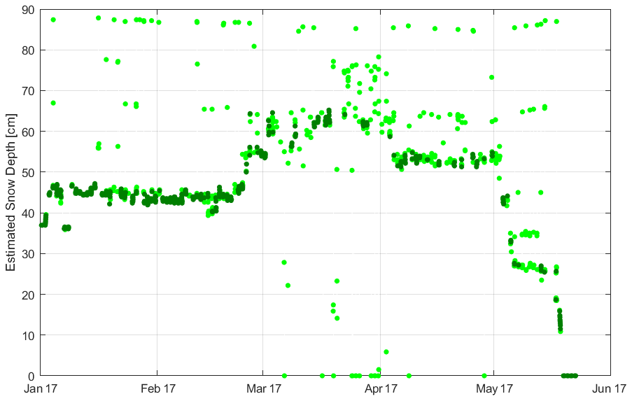
Figure 2 Sodankylä peatland – smoothing algorithm correction of the FMIPROT applied to the snow depth estimate in the first half of 2017. In light-green dots we report the snow depth originally estimated by the FMIPROT using T_s=70 and σ=5, with dark-green dots being the corrected snow depth time series.

Finally the final snow depth time series were defined: the same correction (points 1 and 2) was repeated for each snow depth time series with five different values of parameter σ, from 1 to 5, which can be called SD_C i(t), where C means corrected and i goes from 1 to 5. The advantage of having five runs was the possibility of comparing the single value of one run SD_C i(t) with the mean of the other four, classifying the first as NaN if the difference was more than 0.001 m. In this way one single value was defined as reliable only if more or less the same value was observed in the other four cases. The following condition is given as a summary:

$$\begin{array}{}\text{(7)}& \begin{array}{rl}\text{if}& (\left|{\text{SD}}_{\mathrm{C}i}\left(t\right)-{\displaystyle \frac{\mathrm{1}}{m}}\sum _{j\ne i}{\text{SD}}_{\mathrm{C}j}\left(t\right)\right|>\mathrm{0.1}\mathrm{cm}),\\ & \text{then}{\text{SD}}_{\mathrm{C}i}\left(t\right)=\text{NaN},\end{array}\end{array}$$

where m is equal to 4, i can take a value from 1 to 5 and j must be different from i. In this case m can assume values from 1 to 5 depending on how many values are different from NaN or 0.

Then, the “mean snow depth time series” was obtained as the mean value of the five SD_C i(t) values as

$$\begin{array}{}\text{(8)}& {\text{SD}}_{\mathrm{MEAN}}\left(t\right)={\displaystyle \frac{\mathrm{1}}{n}}\sum _{i=\mathrm{1}}^{\mathrm{5}}{\text{SD}}_{\mathrm{C}i}\left(t\right).\end{array}$$

The mean snow depth time series may still contain not-a-number values. In the case that there is not a long time period with lack of data, not-a-number values were reclassified as the first previous valid value:

$$\begin{array}{}\text{(9)}& {\mathrm{\text{if SD}}}_{\mathrm{MEAN}}\left(t\right)=\text{NaN},\text{then}{\text{SD}}_{\mathrm{MEAN}}\left(t\right)={\text{SD}}_{\mathrm{MEAN}}(t-t_f),\end{array}$$

where t_f is the number of time units before t where a valid snow depth value is available. It is important to underline that this condition works well only if images have a fine temporal resolution and small periods with lack of data. Figure S4 shows with colored dots the five corrected time series obtained with a fixed brightness threshold T_S and for different values of parameter σ from 1 to 5, after applying the removing-bias procedure previously defined (points 1 and 2), whereas the SD_MEAN time series as a result of points 7 and 8 is shown with black dots and a black line. The period of analysis was the first half of 2017, and images are those collected from the Sodankylä peatland camera. Focusing on the SD_MEAN time series, it was shown that, despite the original runs being characterized by lack of data or NaN values, a complete hourly time series was defined. This procedure can give better results if there are images with a high temporal resolution (less than 1 h), because a high drop was not observed between two subsequent values in the case of high melting or snowfall rates, making the discarding phase much easier. Within the “Results” section, this procedure is evaluated in terms of accuracy and efficiency.

To better understand if this method is comparable in terms of accuracy and efficiency to the most common ones available in the literature, two indices were calculated: root mean square error (RMSE) and Nash–Sutcliffe efficiency (NSE). Those indices compared results obtained by the FMIPROT, which will be indicated with the subscript “Sim”, with the observed snow depth values indicated with the subscript “Obs”. The last one was obtained by image inspection for all the three case studies. In the future, we plan to also compare results with in situ measurements. The definition of the two above-mentioned accuracy parameters are given as follows:

$$\begin{array}{}\text{(10)}& {\displaystyle }\text{RMSE}=\sqrt{{\displaystyle \frac{\mathrm{1}}{n}}\sum _{i=\mathrm{1}}^n{\left({\text{SD}}_{\mathrm{Sim}}\left(i\right)-{\text{SD}}_{\mathrm{Obs}}\left(i\right)\right)}^{\mathrm{2}}},\text{(11)}& {\displaystyle }\text{NSE}=\mathrm{1}-{\displaystyle \frac{\sum _{i=\mathrm{1}}^n{\left({\text{SD}}_{\mathrm{Sim}}\left(i\right)-{\text{SD}}_{\mathrm{Obs}}\left(i\right)\right)}^{\mathrm{2}}}{\sum _{i=\mathrm{1}}^n{\left({\text{SD}}_{\mathrm{Obs}}\left(i\right)-\stackrel{\mathrm{‾}}{{\text{SD}}_{\mathrm{Obs}}}\right)}^{\mathrm{2}}}},\end{array}$$

where i means the temporal resolution, n is the total number of simulated values, SD_Sim is the simulated snow depth, and SD_Obs the observed one (obtained by visual inspection of images). Moreover, $\stackrel{\mathrm{‾}}{{\text{SD}}_{\mathrm{Obs}}}$ is the mean observed value.

The RMSE allows us to calculate how much the single snow depth estimated value is different from the observed one, in average terms inside the whole observation period. It will be used to check the result's accuracy.

The NSE compares the residual variance (numerator) with the observation variance (denominator). An efficiency value of 1 corresponds to a perfect match, but also values from 0 to 1 indicate that results are better predictors than the mean observed value. Generally, to indicate a sufficient quality has been suggested, NSE values greater than a threshold from 0.5 to 0.65 are used.

Unfortunately, this coefficient is sensitive to extreme values, so it is not optimal in the case of observed values with high biases.

3 Case studies

3.1 Sodankylä peatland

As a first case study, we considered the Sodankylä infrastructure, which monitors boreal and sub-arctic environmental and climate processes from below the surface to the upper limits of the atmosphere and to space weather phenomena (Fig. S1). In particular we referred to the images from the MONIMET Camera Network (Arslan et al., 2017; Peltoniemi et al., 2018; https://monimet.fmi.fi, last access: 13 January 2021). In Sodankylä, there are a lot of cameras, but we selected the peatland one because it was not affected by snow canopy interception; it is located in the prairie; and it does not suffer from very strong windy conditions, so the relative position between camera and stake remains the same. In addition, at the same site, there is also an automatic weather station as reported in Fig. S1.

Images were collected at a 30 min resolution from 08:00 to 18:00 LT, but generally in winter the first three images and those from the hours after 15:30 are totally dark, since the retrieval of snow depth strongly depends on their clarity. It was decided to limit the use of images within a period of about 6 h with a time resolution of 30 min. Images available are from between 6 November 2015 and 28 April 2019.

The camera was located in front of a white snow stake with 1 cm spaced black markers. The distance between camera and stake was 4.16 m, and between camera and weather station it was 222 m. The distance between camera and stake affected the resolution of the snow depth retrieval because the algorithm cannot detect anything less than 1 cm. Each image has 2592×1944 pixels with horizontal and vertical resolutions of 96 dpi. For images collected in the years 2015 and 2016, more stakes (two or three depending on the period) were deployed at different distances from the camera. The positioning of more than one stake enables us to study the snow depth spatial distribution and also to compare the estimations between different stakes.

An ultrasonic snow depth sensor, available at the test site, collected data at a 1 min time resolution, used to validate and compare the results of the time-lapse photography. Generally, ultrasonic measurements suffer from a lot of noise due to the conversion of the travel time of the emitted and retrieved signals or to the grass above the ground. A correction was automatically implemented and was based on air temperature data. To compare the results and reduce the noise, we defined a snow depth value every 30 min. This dataset is available at https://litdb.fmi.fi/suo0003_data.php (last access: 13 January 2021), for the period 3 November 2011 to 27 March 2019. Having a fine temporal resolution and no lack of data for a long period, these snow depth measurements could be considered a valid reference to test our method. Moreover, Finnish Meteorological Institute (FMI) personnel planned weekly field campaigns with the aim of retrieving snowpack conditions from 3 November 2011 to 28 April 2015. They measured snow water equivalent, snow density and snow depth.

The ultrasonic snow depth measurements were compared with the manual ones, over the overlapping period of observation, 2011–2015, in order to see how the ultrasonic measurements performed in comparison to the manual ones. In order to reduce the noise of ultrasonic measurements, they were aggregated at an hourly resolution. Figure 3 gives the comparison between manual measurements (red dots) and ultrasonic one (dark dots). Focusing on the years 2011 and 2014, an agreement was found between the two methods of measurement, whereas in 2012 and 2013, some differences were seen. In 2012, the ultrasonic snow depth sensor was characterized by some problems, which prevented the measurements from being performed correctly. In 2015, the ultrasonic snow depth sensor measured the highest snow depth peak which was smaller than the manual measurements. This situation was vice versa in 2013. In both 2013 and 2015, the accumulation season (typically winter) and the melting one (typically late spring) show a good agreement although there were differences in estimation peak values. In addition, we highlight that the snow depth ultrasonic sensor was not affected by a persistent under- or overestimation that can be a warning of instrument drift.

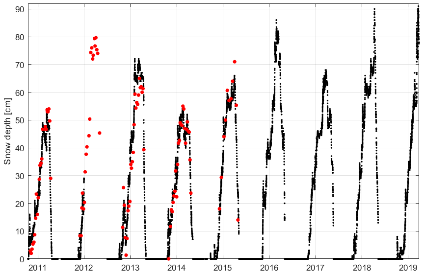
Figure 3 Sodankylä peatland snow depth hourly time series collected by Campbell ultrasonic snow depth sensor (black dots) and manual measurements (red dots).

Caused by the poor resolution of the manual measurements and some periods with lack of data, only 105 values were compared. In addition, all the snow depth data series (ultrasonic, manual and FMIPROT estimations) cannot be used in comparison because manual measurements were not available when the camera was installed. Finally, for each day in which there were both manual and ultrasonic snow depth sensor measurements, an RMSE was calculated equal to 0.045 m. With this, reliable ultrasonic measurements were retained and used as reference for the years between 2015 and 2019 to compare the snow depth retrievals from time-lapse photography. Table 2 reports information about sensors, the period of observation and the time resolution used.

Table 2 Data description related to each case study with observation period and temporal resolution.

3.2 Gressoney-La-Trinité

The second case study is located in the Aosta Valley region (Italy), at an altitude of 1850 m a.s.l. where since 1927 the Italian Meteorological Society has measured the snow depth on the ground by rulers. This site can be considered a historical meteorological observatory of snow depth retrieval in Italy due to the long-term data availability. In addition, from 2002 the autonomous Aosta Valley region has had an automatic weather station, with which is measured precipitation (without heated pluviometer), temperature and relative humidity.

Figure S2 shows (from the right to left) Aosta Valley inside the Italian territory, the Gressoney-La-Trinité Dejola site, and a picture of the snow stake inside the meteorological observatory. Recently, from 1 September 2013 AINEVA (Interregional Association for Snow and Avalanche problems coordination) has positioned a snow stake with 10 cm spaced dark markers. The total length of the stake is 2 m, and it has a width of 10 cm. The camera is a Siap Micros model, with a height of 2 m above ground level (a.g.l.) and 10 m distance from the stake. As shown in Fig. S2, the snow stake was not positioned specifically for the remote sensing image-processing purpose, and it is affected by a non-optimal geometrical configuration because there is a different distance between the camera and the top and the bottom of the stake. The importance of the positioning and optimal geometrical configuration is described later in the section related to the discussion of results (Sect. 5).

AINEVA, from 1 September 2013, saves images from the camera at an hourly resolution from 06:00 to 18:00 LT. Especially in the winter season some images appear totally dark, so it was decided to use only those taken from 08:00 to 15:00. Dimensions of the images are 1280×960 pixels, with horizontal and vertical resolutions of 96 dpi.

AINEVA operators made the visual estimation of the snow depth, saving the snow depth value accumulated on the ground in a spreadsheet file. From personal communication with people who made these measurements, the camera is affected by a parallax effect, due to the relative distance between the height of the camera and the bottom of the stake. In addition, the real snow depth value cannot be retrieved simply reading the first marker not covered by snow because there is a heat transfer from the stake to the snowpack due to conduction and reflection of incident solar radiation. Therefore, operators reporting measurements considered this effect, defining the real snow depth obtained as a cross between snow stake markers and a virtual line which links the snowpack accumulated on the ground at the left and right side of the stake (Fig. 4a).

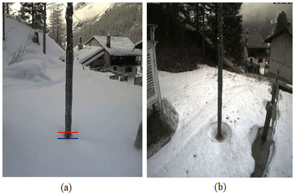
Figure 4 (a) Images from Gressoney Dejola camera, taken at 08:00 LT on 9 February 2017. In red we marked the AINEVA operator estimation, and in blue we marked the first selected marker from the FMIPROT algorithm. (b) Image from Gressoney-La-Trinité Dejola camera on 13 April 2016 which shows the high melting rate close to the stake.

In this way AINEVA operators defined two snow depth values for each day at 08:00 and 14:00. We decided to use these values as a reference to compare the results obtained by our procedure (these values are reported with black dots in Figs. 9 and 10).

Because our aim is to compare and validate the snow depth values retrieved from digital images, it was decided to discard years in which the reference value cannot be detected directly by visual inspection of images, focusing in the period between November 2014 and December 2017. As a period of validation, we selected the period between 2018–2019, as reported in the “Results” section.

3.3 Careser Dam

The third case study is located in the Trentino region (Italy), the Careser Dam, at an altitude of about 2600 m, near Careser Glacier. The Civil Protection Agency installed a snow camera in 2014 with the aim of collecting snow data for hydrological purposes.

In this region, there are a lot of sites in which manual measurements are taken every day. In fact, there are a lot of dams and ski areas, where private companies have an interest in monitoring the snow availability during the winter season. In addition, AINEVA and Meteotrentino collected and disseminated daily information related to the snowpack such as snow depth and density to define the avalanche risk. Unfortunately, in the Trentino region, as well as in the whole Italian territory, there are not many snow cameras which can be used for our study. Figure S3 gives the location of Careser Dam and an image from the camera.

Despite the fact that the camera was not specifically installed for remote sensing image processing and the retrieval of snow depth, we used this to test the potential of the time-lapse photography. The camera was located at 3 m a.g.l., with a distance of about 6.5 m from the graduated stake which has a width of 15 cm and is colored in yellow with 1 cm spaced markers. The total length of the stake is 2 m. The camera model is Axis 214 PTZ, with a semispherical protection in Plexiglas. Unfortunately, the temporal resolution is poor in this case, as operators collected only four images per day at 05:00, 08:00, 11:00 and 14:00 LT. In most of the cases the first one at 05:00 appears totally black, so we have discarded it.

The observation period goes from 1 January 2014 to 31 December 2018, but in some periods, there was a lack of data due to bad atmospheric conditions in which strong wind produced a camera rotation resulting in images without the snow stake. Other images which had to be discarded are those in which snowflakes remained on the camera's objective, making images totally grey or the snow stake partially invisible. These problems occurred when the camera was not protected properly. In fact, in most of the places where this technology was implemented, the camera was placed in a small wooden box. In addition, sometimes, the snow stake is positioned near a fence, which, especially in the melting season, enables percolation toward the stake, which increases the snowmelt. After summer 2017, AINEVA replaced the camera with one with an increased image resolution. As a result of this change, the relative position between the camera and stake was not the same for the whole observation period.

Regarding images, from 2014 to the middle of 2017, they are 768×576 pixels with a horizontal and vertical resolution of 96 dpi. Starting from November 2017, the number of pixels of each image was increased to 1920×1080.

Unfortunately, in this case there was no snow depth sensor or snow field manual measurements; we made visual estimations of the snow depth, simply opening each image and looking at the snow stake markers in order to have a reference value to compare our estimations. In many cases the visual estimations were not so easy to make because an amount of snow remained attached to the snow stake. Another problem is the differential melting rate between the snowpack close to the stake and at a distance of more than 1 m. This is caused by the high snow stake reflectivity related to the incoming sunlight, heat transmitted by conduction and the water percolation from the top to the bottom of the stake. This effect is hardly quantifiable and depends on the atmospheric conditions. Therefore, for the “visual estimation”, this time series is also affected by noise which can be quantified as 5 cm. The visual estimation is obviously time-consuming because we have to open and read each image, but we are quite sure that this kind of estimation is not affected by outliers or unreliable values. We also have to point out that the visual estimation is subjective, and the same image can lead to different values estimated by different observers. Figure 11 shows the snow depth daily time series obtained from visual estimation with black dots for the period between 1 November 2015 and 31 December 2018.

4 Results

As a general comment, we can say that the algorithm of retrieval may fail in snow depth detection when the geometrical configuration of the camera and the stake were not defined for this aim. For the two Italian case studies, the cameras were installed only for a rough evaluation of snow depth and were not intended for the quantitative monitoring of snowpack dynamics.

In the Sodankylä peatland case study, we used an ultrasonic sensor, manual measurements and visual estimations from images as reference data for comparison. For the two Italian case studies, we must refer only to the visual estimations from images. In particular for Careser Dam, we did not have any additional information, but for the Gressoney Dejola, the Italian Meteorological Society visually estimated snow depth, with a “critical” snow depth definition, which means that they took into account the high melting that occurred close to the stake and tried to remove the parallax effect due to the different height between the camera and the top of the stake.

4.1 Sodankylä peatland

In this case the algorithm works well because the stake was positioned closer to the camera and the images have more pixels showing the stake and appear clear, without high or low values of brightness and reflectivity. Moreover, it was positioned inside a small housing which could protect it against strongly windy conditions and the possibility of obstruction of the camera's view caused by snowflakes. The stake much closer to the camera was enough to retrieve snow depth values with an adequate temporal resolution and geometrical accuracy. As mentioned in the data description section (Sect. 3), here we only had images from after 2014, so to check the reliability of the FMIPROT snow depth algorithm, we could only use the ultrasonic snow depth sensor, positioned close to the camera, because we did not have any other information, like manual measurements.

The comparison between retrieved and observed values of snow depth is reported in Fig. 5, related to the period from 6 November 2015 to 27 March 2019. Specifically we plotted retrieved values in blue dots, the visual estimation of images with red dots and Campbell ultrasonic measurements in black dots. The snow depth time series is correctly reproduced, and good agreement between retrieved values and measurements has been found.

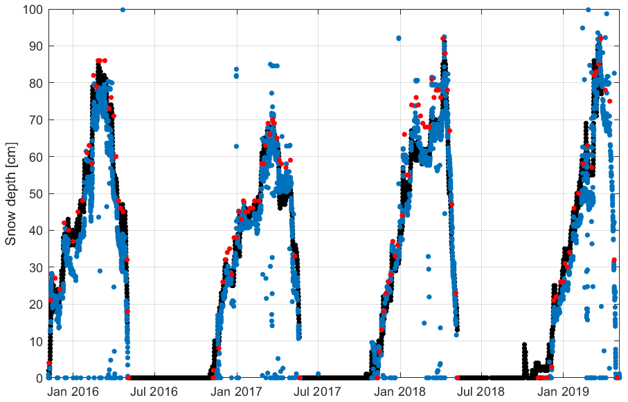
Figure 5 Sodankylä peatland: snow depth estimation comparison – ultrasonic measurements (black dots), estimated by the FMIPROT (blue dots) and visual observations (red dots).

In general, visual estimations provide higher values, so we can observe an underestimation of the ultrasonic snow depth sensor and FMIPROT retrievals. Here it is interesting to highlight that the temporal resolution of FMIPROT retrievals is 30 min, within the daylight hours which start from 09:00 and end at 15:00 LT. Ultrasonic sensors measured snow depth at a 10 min resolution, and visual estimations were reported weekly. Therefore, if the images were clear and without a long period with lack of data, we could build a snow depth time series with a high temporal resolution. Regarding the accuracy, we calculated the RMSE and NSE, comparing FMIPROT retrievals with ultrasonic snow depth measurements and the visual observation of images.

Comparing FMIPROT retrievals and ultrasonic snow depth sensor measurements, we obtained ${\text{RMSE}}_{\mathrm{FMI}-\mathrm{US}}=\mathrm{0.096}$ m and ${\text{NSE}}_{\mathrm{FMI}-\mathrm{US}}=\mathrm{0.799}$, while comparing FMIPROT retrievals with visual observation of images, we found ${\text{RMSE}}_{\mathrm{FMI}-\mathrm{VO}}=\mathrm{0.085}$ m and ${\text{NSE}}_{\mathrm{FMI}-\mathrm{VO}}=\mathrm{0.881}$. Visual observations are considered much more reliable than the ultrasonic measurements because they were obtained by a direct reading of the markers' stake in contrast to the ultrasonic sensor, which was positioned much nearer to the camera and very far from the stake. We also have to highlight that the comparison with the ultrasonic snow depth sensor was performed at an hourly resolution, despite those data with visual inspections having a weekly resolution. Another interesting issue is the number of misclassifications, or the inability of the FMIPROT algorithm to give a snow depth real value. In this case, NaN values were assigned to 2.91 % of the images.

Building the snow depth time series in the first half of 2017

Thanks to the 30 min temporal resolution of the images and a period without lack of data, we tested the “smoothing” procedure defined in Sect. 2 inside a 6-month period, in the first part of the year 2017, to obtain a complete snow depth time series without NaN values. Moreover, we repeated retrievals, fixing the threshold parameter at 70 and varying the Gaussian filter parameter σ from 1 to 5. The final snow depth time series was obtained by calculating the average of five retrievals. In Fig. 6, we show the comparison between the FMIPROT snow depth time series, visual estimation from images and the ultrasonic snow depth measurements.

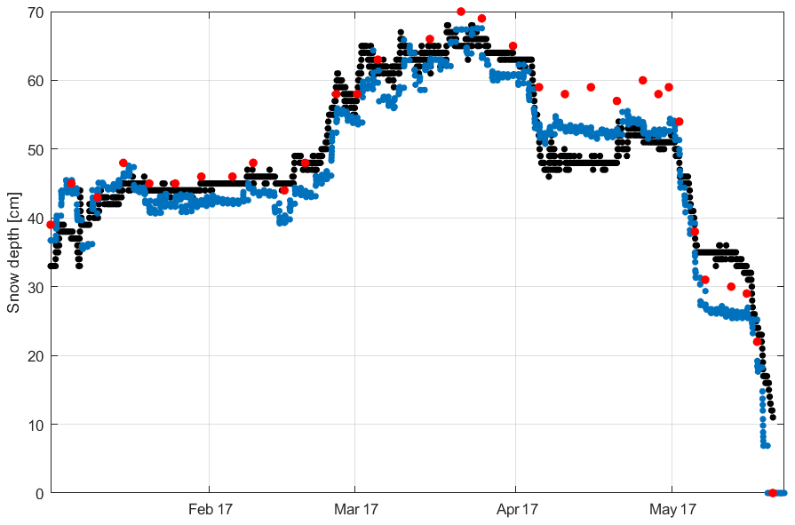
Figure 6 Sodankylä peatland: comparison between visual estimations (red dots), ultrasonic measurements (black dots) and the FMIPROT estimations (blue dots) in the first half of 2017.

As we can see from Fig. 6, we can build the snow depth time series with a high temporal resolution and with high accuracy. As previously, considering as reference the visual snow depth estimations, we found for the ultrasonic snow depth sensor RMSE_US=0.052 m and NSE_US=0.881, while for the FMIPROT retrievals RMSE_FMI=0.039 m and NSE_FMI=0.917. With these values we can say that FMIPROT retrievals are much more accurate and efficient compared to the ultrasonic snow depth sensor values, and this happened especially in January and April.

These results are important because we can not only retrieve a single value of the snow depth with high accuracy but also build a snow depth time series, without lack of data. Moreover, these results were obtained without a data assimilation procedure, which in most of the cases “force” the results by knowing the real snow depth value. In addition, this procedure is completely automatic and not time-consuming.

4.2 Gressoney-La-Trinité

Regarding the snow depth observed values, which will be used to compare our results, AINEVA operators defined three values with a visual inspection of the images at 08:00, 14:00 and 21:00 LT on each day in the period from 4 November 2014 to 31 December 2017. The last one (21:00) is equal to the last visible image for each day (AINEVA operator, personal communication, 2019), so, as it is not known exactly to which time those measurements referred, we avoided using those. For this reason, having only two reference values for each day, to estimate the snow depth with the FMIPROT, we decided to select only two images per day, which correspond to the same hours (08:00 and 14:00 LT). In most cases images appeared clear, without any lack of data, and defining the threshold values as mentioned in the algorithm section (Sect. 2.1), we made the computations using the FMIPROT.

In addition, as mentioned in Sect. 3, AINEVA operators defined a visual observation that considered the parallax effect, so the algorithm detection of the first visible marker could be different from this visual estimation as shown in Fig. 4a.

In this case, we had to define two different parameterizations to make retrievals due to the parallax effect, caused by the different distance which exists between the top and the bottom of the stake to the camera. Here the relative position between camera and stake was not optimal, because the camera was not positioned, in terms of height, at the middle of the stake. This situation leads to a greater number of pixels corresponding to a marker for the top of the snow stake compared to the bottom. As a consequence, considering a unique ROI, the parallax effect would cause a strong underestimation. In conclusion, when the snow depth is less than 0.3 m we used the following parameterization: L_s=0.3 m, T_S=70 and σ=4. When the snow depth is greater than 0.3 m we used L_s=1.2 m, T_S=70 and σ=4.

Comparing the retrievals obtained by the FMIPROT and values given by operators, we found that there was a strong difference between the two as shown in the scatterplot in Fig. 7. This showed a constant underestimation of the FMIPROT algorithm results. For this reason, in the following we will define a constant bias to correct our estimations. In addition, we calculated the ratio between observed and estimated values, as shown in Fig. 8, in which we can see that the lowest values are those affected by the greater underestimations; this fact was expected because, due to the higher melting near the stake, if the snowpack had accumulated on the ground, the first visible marker could be near 0. In other terms when the real snow depth on the ground is near 0.1 m, the retrieval algorithm can fail. To better explain this fact, we also show an image related to the data from 13 April 2016 (Fig. 4b). Here the estimated snow depth reported by the operator was 0.24 m, but the algorithm gives 0.052 m because the stake was almost totally visible from the camera angle. As we will discuss in the following section, when the snow depth is less than 0.1 m, those images and this geometric configuration did not allow us to adequately estimate snow depth. But we have to highlight that this is due to the imperfect design of the relative position between camera and stake and not to the algorithm incapability.

Figure 7 Gressoney-La-Trinité Dejola: scatterplot between FMIPROT-estimated (before correction procedure) and observed values.

Figure 8 Gressoney-La-Trinité Dejola: ratio between observed and estimated snow depth values in the calibration period.

These differences between visual estimation and the FMIPROT results seem to be constant, and we decided to calculate the mean error, splitting the snow depth values between those greater than 0.3 m and others.

Considering observed values more than 0.3 m, we found a mean error equal to 0.12 m, whereas for the values greater than 0.3 m, we found a mean error of 0.19 m.

Because our aim was to define a method to estimate snow depth which can be carried out automatically in the future without the long procedure of visual estimation from images, we defined a corrected snow depth retrieval time series in this way:

• -

  if SD_Sim(t)<0.30 m, then ${\text{SD}}_{\mathrm{Sim}\mathrm{Cor}}\left(t\right)={\text{SD}}_{\mathrm{Sim}}\left(t\right)+\mathrm{0.12}$ m, and

• -

  if SD_Sim(t)>0.30 m, then ${\text{SD}}_{\mathrm{Sim}\mathrm{Cor}}\left(t\right)={\text{SD}}_{\mathrm{Sim}}\left(t\right)+\mathrm{0.19}$ m,

where SD_Sim(t) is the original snow depth time series obtained by FMIPROT retrievals and SD_Sim Cor(t) is the corrected values obtained by adding a correction factor (operator specific).

To verify visually the method's accuracy, in Fig. 9, we reported the comparison between observed and retrieved values before and after correction. The new snow depth seems to be much closer to the observed one after this correction procedure.

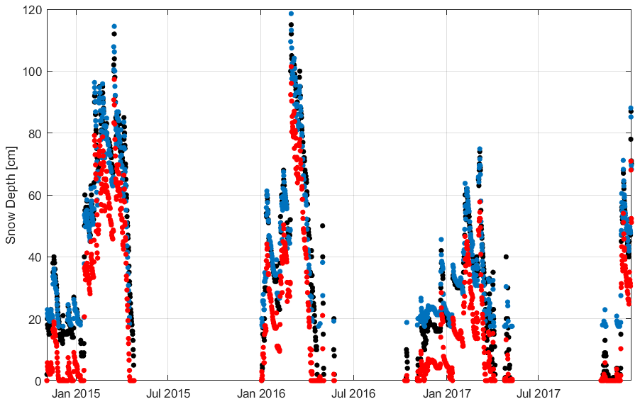
Figure 9 Gressoney-La-Trinité Dejola case study: comparison between snow depth daily time series retrieval from camera images, through visual estimation carried out by AINEVA operators (black dots) and estimated snow depth after (blue dots) and before (red dots) correction, in the calibration period.

We also calculated RMSE and NSE before the correction (BC) and after the correction (AC). In the case of considering the original snow depth retrieval, the accuracy parameters RMSE_BC=0.171 m and NSE_BC=0.609 were obtained. After the correction procedure we increased the performance of retrievals, obtaining these accuracy values: RMSE_AC=0.052 m and NSE_AC=0.963. In addition, it is important to highlight that the number of algorithm failures (i.e., when snow depth is equal to NaN) is only 1 among 1054. Therefore, the percentage is less than 0.1 %.

Moreover, to test the model reliability, we selected images between 10 November 2018 and 3 May 2019. Unfortunately, this period is not optimal to test our model because most of the time the snow depth on the ground was less than 0.1 m. Since we were interested in validating the method and checking if the algorithm can retrieve the snow depth with enough accuracy, we considered only those values greater than 0.1 m.

With this aim, the FMIPROT was run, and using the correction factor previously defined, the results were compared with the observed snow depth, shown in Fig. 10. RMSE=0.062 m and NSE=0.771 were found. These results are comparable to those reported for the period 2015–2017.

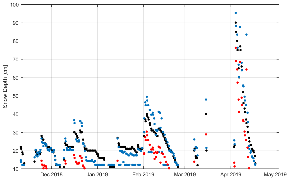
Figure 10 Gressoney-La-Trinité Dejola: comparison between snow depth daily time series retrieval from camera images, through visual estimation carried out by AINEVA operators (black dots) and simulated snow depth after (blue dots) and before (red dots) correction, in the validation period (November 2018–May 2019).

This case study was interesting because, even though the geometrical configuration was not optimal, most of the images were discarded and high melting close to the stake occurred, by studying the results in a critical way and simply applying a constant correction factor, snow depth values can be estimated with good accuracy.

In this section, the correlation plot helped us to define the method to correct the data, trying to minimize FMIPROT estimation errors. In the Sodankylä case study, measurements were corrected with another approach that is shown in Fig. S4, defining an ensemble of runs with different parameters. In this way two different solutions were shown to make our results more reliable.

4.3 Careser Dam

In this case study, we have only three visible images per day at 08:00, 11:00 and 14:00 LT. In addition, in the last year, the camera was broken, so we could not use images to retrieve the snow depth. For these reasons, the period between 1 January 2016 and 11 June 2018 was selected.

As in Gressoney-La-Trinité Dejola case study, here we also could not compare the FMIPROT algorithm estimations with manual or ultrasonic snow depth measurements. Thus, we referred to the visual estimation of images to validate our results. For most of the available images we estimated the snow depth visually by inspecting each image and recording in files the height of the first visible marker above the snowpack layer. These measurements were used as a reference to compare the results. As it was said before, this method is not optimal, and it is affected itself by an error which can be quantified as 0.05 m. It is also good to note the change in the camera in summer 2017; this is the reason why different parameters had to be chosen before and after that date. In fact, previous images have a worse pixel image resolution, but the camera's view is much more focused on the stake. After summer 2017, a better pixel image resolution can be observed, but camera zoom decreased and the stake appeared much farther from the camera. In addition, it is important to highlight that a much greater camera stability occurred in the first period compared to the second one.

Initially there were worries about results because this site is located at an altitude near 2600 m, in a wind-prone area and with very poor climatic conditions in winter in terms of temperature and high snowfall. In addition, AINEVA and Meteotrentino collected images at 08:00, 11:00 and 14:00 LT, and especially in spring the last one is not optimal because of high sunlight levels.

In Fig. 11 a comparison is shown within the observation period: 1 January 2016–31 December 2018.

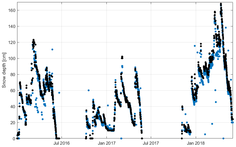
Figure 11 Careser Dam case study. Comparison between snow depth retrieved by the FMIPROT (blue dots) and through visual estimation of images (black dots) for the period 1 January 2016–1 June 2018.

These results were obtained defining the set of parameters as L_s=2 m, T_S=67 and σ=10, for the period until June 2017. Afterward, the set of parameters was changed to L_s=2 m, T_S=68 and σ=3.

The accuracy indices were calculated between visual inspection and FMIPROT retrievals, obtaining these results: RMSE=0.108 m and NSE=0.916.

Here it is seen that the algorithm was very successful, especially within the hydrological year 2016–2017 in which snow depth was not very high and there were few snowfall events and subsequent rapid melting. Despite this site not being established for the purpose of snow retrieval, we obtained good results in terms of accuracy. The only problem here was the camera use limitation due to the poor atmospheric conditions which characterized the mountain region. It is also good to mention that, despite the temporal resolution being poor, just three images per day, it seems that the snowpack temporal variability can be followed with high accuracy. It would probably be better to increase the temporal resolution, to allow us to have a snow depth time series with an hourly resolution. The algorithm detected the snow depth well because markers of the stake were larger than those in the other case studies; here the stake had a width of 0.2 m. Therefore, by applying a Gaussian filter parameter of greater than 1, we can avoid misclassification and correctly detect the stake's marker shapes. The percentage of NaN over total images was calculated, which was equal to 1.5 %.

5 Discussion

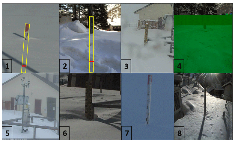
Here we analyze firstly the causes of algorithm failure and secondly configuration issues of the camera–stake system. As shown previously, especially when images had an hourly resolution, in some cases the retrieval algorithm could not correctly provide the snow depth value. Here we explain why that could happen and in the next section how we can solve these problems by improving the geometrical configuration. In the analysis of the three case studies we found eight sources of algorithm failure illustrated in Fig. 12. Now we describe each of them:

• 1.

  Shadows projected on the snowpack, which fall inside the ROI. In some cases, especially when the sun was behind the camera and when some buildings or an automatic weather station or trees were located near the camera, shadows on the snowpack surface were detected as a marker by the algorithm picking phase. This happened in all the three case studies. Panel 1 of Fig. 12 shows this source of error, in which the sunlight highlighted the automatic weather station located near the camera, projecting its shape above the snowpack. This induced the reading of the shadow's position as a first visible marker above the ground, strongly underestimating the snow depth that, in this case, must be near 1 m. To avoid this problem, we suggest removing all the possible sources of shadows near the stake and camera.

• 2.

  Footprint, which alters the snowpack in front of the stake and appears inside the ROI (panel 2 of Fig. 12). The same effect as that previously explained was caused by an alteration in the snowpack surface. Animals, people or drops falling from the trees can alter the surface, creating some discontinuities, which can be classified as a marker by the counting-pixel-algorithm phase. To avoid this problem, we suggest protecting the area close to the stake, making it inaccessible.

• 3.

  Obstruction of the camera's view (panel 3 of Fig. 12). Especially in the case of extreme snowfall events, snowflakes can partially or totally cover both the camera's view and some part of the stake, obscuring the first clean marker which must be visible to correctly detect the snow depth. Here the only suggestion is to protect the camera against rainfall and snowfall events, positioning it inside a box which can be made of wood or steel with one side open or with a transparent window (Plexiglass or glass).

• 4.

  Pixel reflectance alteration. Due to excessive exposure to direct sunlight of the camera's objective, some images lost their true colors, becoming unreadable. This problem occurs rarely (panel 4 of Fig. 12), so it is difficult to find a geometrical design which can avoid this problem.

• 5.

  Rotation of the camera's view (panel 5 of Fig. 12). Extreme windy conditions can cause the camera's rotation, and the stake can disappear from the camera's view. To maintain the camera in the same position, it must be positioned inside a wooden or steel box as previously explained (point 3).

• 6.

  Blurred or opaque images (panel 6 of Fig. 12). In some cases, it can happen that pixels cannot be distinguished from others, so from the algorithm point of view markers appear to be the same as the background, making their counting impossible.

• 7.

  Wind snow drift (panel 7 of Fig. 12). Strong wind velocity can carry snowflakes from the ground to the stake markers. In this case the markers became white and indistinguishable from the white background.

• 8.

  Direct sunlight in front of the camera and high reflectance above the snowpack (panel 8 of Fig. 12). In this case it is not so clear why the algorithm failed and what kind of protection has to be defined to avoid this problem.

Figure 12 Sources of algorithm failing.

Studying in detail the results and causes of algorithm failure, we tried to define the proper geometrical configuration between the camera and stake, highlighting the main characteristics which each single component must have:

• -

  Relative position between camera and stake. The better configuration required that the snow stake be positioned as close as possible to the camera. In this case the algorithm can detect markers' positions more easily because more than 1 pixel can discretize one single marker. We suggest a maximum distance of 10 m. The camera's height has to be set in terms of reducing the parallax effect, so a common stake of 2 m is enough for a camera's height of 2 m. The rotation angle of the camera must guarantee perpendicularity, avoiding pixel size distortion. Between the camera and stake it is better to remove all the possible obstructions such as branches of trees which can be identified as markers.

• -

  Snow stake. We suggest a wooden stake, to reduce conductive heat transfer between the stake and snowpack, limiting the sunlight reflectance from the snow. The background color must be yellow with black markers with 0.01 m spacing. The stake width must be 0.2 m, and markers must cover half of that. It is better to make the area near the stake inaccessible, to avoid problems of snowpack alteration caused by human or animal footprints. To increase stake stability, it is better to fix it on a steel plate which in turn can be fixed on the ground (preferably on the rock) with at least four expandable anchor sleeves with quick-setting cement. The ground or rocks surrounding the stake must be as flat as possible to avoid gravitational movement of the first snowpack level and the possibility of a horizontal translation of the stake.

• -

  Camera. The image resolution is not so important if we respect an adequate distance from the stake; however we suggest using a camera with a high image resolution, say 5 MP. It is mandatory to protect the camera against wind and precipitation events, positioning it inside a wooden box of which one side must remain either open or closed with a plastic or glass window.

• -

  Connection with monitoring service. If characteristics of the snowpack are required in real time, there should be a permanent connection between the camera imaging storage and the monitoring service center. This can be power alimented thanks to a solar panel.

• -

  Other instrumentation or field measurements. To cross-correlate and validate algorithm estimations periodically, it is mandatory to compare algorithm estimations with manual measurements obtained by planned field campaigns. Additionally we suggest placing (a) an automatic weather station with a temperature sensor to remove some misclassification (for example the highest melting rate if the temperature was not more than 0 ^∘C) and (b) an ultrasonic snow depth sensor, which can be used when the algorithm cannot detect snow depth values in the correct way. The last suggestion can be that of positioning more than one stake inside the camera's view and comparing the algorithm estimations, defining different regions of interest selecting each stake one by one.

Generally, working with images to detect if 1 pixel could be classified as snow, we defined a brightness threshold of 127. But in the three case studies it was found that a brightness threshold of between 60 and 75 is better to detect the snowpack layer (probably because we were more interested in the marker's shape detection despite the single-pixel classification). In addition, it was found that in most of the cases a Gaussian filter sigma of 1 was good enough to correctly retrieve markers' shapes and positions. Moreover, to define a reliable snow depth time series, it is better to repeat the analysis with different parameter configurations and take the mean value among them to remove all possible errors which can affect a single time series as explained for the Sodankylä peatland case study.

In addition, for the first image it is mandatory to have the whole snow stake not covered by snow, because we have to detect the right ROI (region of interest), which must have as the lower bound the ground level without snow. The highest contour level can be defined by the users remembering that it should be much more than the expected maximum snow depth in the accumulation season. Consequently, and coherently with the previous phase, at the ROI identification stage it has to be associated with the real stake length in meters.

6 Conclusions

The main aim of this study was to explore the capability of the time-lapse photography method to retrieve snow depth time series in various snow conditions. Three case studies were considered: one in boreal forest, Finland, and two in the Italian Alps. The first case study was properly designed for retrieving the snow depth by camera images, while in the other two, cameras were set up for other purposes (a simple qualitative monitoring of the snow depth on the ground).

The results showed that, if the images were clear and the relative position between the camera and stake allowed us to detect the stake's markers, the proposed algorithm implemented within the FMIPROT was successful in estimating the snow depth. The agreement between estimations and visual inspection of the images was evaluated with the Nash–Sutcliffe efficiency, which reached values greater than 0.9 for all case studies. To evaluate the accuracy, the root mean square error was calculated, which was higher in the Careser Dam site than in the other two. This can due to (1) the extreme weather conditions at 2600 m a.s.l. which may affect the camera's visibility and (2) the presence of the shadows above the snowpack layer, which can be classified as a stake's marker by the image's segmentation algorithm phase. There is a necessity to define the proper geometrical and parameter configuration for reducing the possible sources of estimation errors. The camera must be positioned at the same distance from the stake's ends, and the stake must be a wooden one of a 15 cm width, with a yellow background color and black markers which cover half of that. The camera must be protected against extreme weather conditions (high wind velocity, intense rainfall or snowfall events) by positioning it inside a wooden or steel box. All possible sources of shadows must be avoided. In the Sodankylä case study, we compared the performances of the proposed algorithm with an ultrasonic snow depth sensor which measured the snow depth near the stake. In terms of NSE and RMSE, we found higher accuracy of the proposed algorithm compared to that of the ultrasonic Campbell sensor, assuming manual measurements as a reference.

In conclusion, we underline some strengths of the proposed algorithm:

• -

  High temporal resolution. Depending on the camera's scan rate and storage data capability, we can build hourly or sub-hourly snow depth time series.

• -

  High accuracy levels. If the geometrical configuration of the camera–stake system and related infrastructure are perfectly designed, the proposed method estimates snow depth with accuracy levels comparable to the most commonly used methods (manual measurements, ultrasonic or optical sensors).

• -

  Reliability. The percentages of algorithm failure are low, and if some outliers are generated, we can easily detect and correct them with a post-processing procedure or simply by opening the image and performing a visual reading of the first visible marker above the snow layer.

• -

  Low cost. This can be considered a low-cost solution with low maintenance costs.

• -

  Remote sensing technique. The approach can be easily extended in remote and dangerous areas such as mountain glaciers or polar regions in which currently there is a lack of data.

Our results indicate that time-lapse photography has good potential to retrieve snow depth time series. Future developments are necessary, such as improving the algorithm for reducing possible misclassifications and errors, and there may be possible upscaling solutions. The time-lapse photography can be a complementary solution used with satellite remote sensing for estimating snow depth automatically and remotely. It can be applied to many other applications such as estimating snowfall events, pluviometer undercatch correction, snowfall and rainfall splitting, estimating reservoir water levels or discharge, estimating glacier melting, and monitoring lake or river water levels in real time in case of floods.