Surges of Harald Moltke Bræ, north-western Greenland: seasonal modulation and initiation at the terminus

Harald Moltke Bræ, a marine-terminating glacier in north-western Greenland, shows episodic surges. A recent surge from 2013 to 2019 lasted significantly longer (6 years) than previously observed surges (2–4 years) and exhibits a pronounced seasonality with flow velocities varying by 1 order of magnitude (between about 0.5 and 10 m d⁻¹) in the course of a year. During this 6-year period, the seasonal velocity always peaked in the early melt season and decreased abruptly when meltwater runoff was maximum. Our data suggest that the seasonality has been similar during previous surges. Furthermore, the analysis of satellite images and digital elevation models shows that the surge from 2013 to 2019 was preceded by a rapid frontal retreat and a pronounced thinning at the glacier front (30 m within 3 years).

We discuss possible causal mechanisms of the seasonally modulated surge behaviour by examining various system-inherent factors (e.g. glacier geometry) and external factors (e.g. surface mass balance). The seasonality may be caused by a transition of an inefficient subglacial system to an efficient one, as known for many glaciers in Greenland. The patterns of flow velocity and ice thickness variations indicate that the surges are initiated at the terminus and develop through an up-glacier propagation of ice flow acceleration. Possibly, this is facilitated by a simultaneous up-glacier spreading of surface crevasses and weakening of subglacial till. Once a large part of the ablation zone has accelerated, conditions may favour substantial seasonal flow acceleration through seasonally changing meltwater availability. Thus, the seasonal amplitude remains high for 2 or more years until the fast ice flow has flattened the ice surface and the glacier stabilizes again.

1 Introduction

Surge-type glaciers are characterized by an alternation of long periods of low flow velocity (several to hundreds of years, quiescent phases) and comparably short periods with velocities increased by at least 1 order of magnitude (1–15 years, active phases or surge events) (Jiskoot, 2011; Benn and Evans, 1998; Bhambri et al., 2017). These rapid changes in ice flow are triggered by internal instabilities and are mostly independent of external influences like weather or climate (Jiskoot, 2011; Benn et al., 2019). Therefore, knowledge about the occurrence and distribution of surge-type glaciers and an understanding of the underlying surge mechanisms are crucial when studying the relationship between climate change and changes in glacier dynamics.

Only about 1 % of the glaciers worldwide are assumed to be surge type (Jiskoot, 1999). Surge-type glaciers normally cluster in certain regions (such as Alaska, Svalbard and the Karakoram) where the conditions are favourable for surge behaviour (e.g. a soft glacier bed and an at least partially temperate regime) (Sevestre and Benn, 2015; Jiskoot, 2011). Some surge-type glaciers are also known in Greenland. For example, clusters of surge-type glaciers in central–western Greenland and central–eastern Greenland were reported by Sevestre and Benn (2015). Apart from these clusters, Hagen Bræ in north-eastern Greenland is assumed to be a surge-type glacier (Solgaard et al., 2020).

Another surge-type glacier isolated from the known surge clusters is Harald Moltke Bræ, a marine-terminating glacier in north-western Greenland. Remarkable changes in the flow behaviour of Harald Moltke Bræ were first documented by Koch (1928) and Wright (1939), who observed an exceptional advance of the glacier front by about 2 km between 1926 and 1928 and inferred that the average surface flow velocity in this interval was at least 1000 m yr⁻¹ (2.7 m d⁻¹). Mock (1966) used the displacement of ice-surface features visible in aerial and terrestrial photographs to show that between 1954 and 1956 the average velocity was about 1 m d⁻¹, 10 times higher than the average velocity between 1937 and 1938. Based on satellite remote sensing, active phases in 1999/2000 and 2005/2006 were documented by Joughin et al. (2010) and Rosenau (2014), and accelerated flow in 2013/2014 was reported by Hill et al. (2018).

The present study was triggered by unprecedented observations of a remarkable flow behaviour of Harald Moltke Bræ, based on the combination of optical and radar remote sensing data. The latest surge lasted from 2013 to 2019, significantly longer than the previous two active phases, 1999/2000 and 2005/2006 (both 2 years). Simultaneously with this surge, there was a strong seasonality with velocities decreasing to the level of the quiescent phase in summer, which has not been observed at Harald Moltke Bræ in this way before. Studying this surge behaviour and its causes may provide new insights into the surge mechanisms of marine-terminating glaciers in Greenland. We provide a detailed overview of changes in the dynamics and the geometry of this glacier between 1998 and 2020. We analyse and interpret the flow behaviour and propose causal processes in the light of previous studies of surge-type glaciers.

The flow of a surge-type glacier during its quiescent phase is typically slower in its lower part than in its upper part. Due to the resulting negative velocity gradient in flow direction, the upper part, called reservoir area, thickens dynamically, while the lower part, called receiving area, thins (Jiskoot, 2011; Benn and Evans, 1998). This pattern reverses in the active phase. When ice flow in the receiving area is enhanced during the active phase, the glacier front may advance rapidly. Most known glacier surges start with an increase in flow velocities in the upper part of the glacier and propagate down-glacier (Raymond, 1987; Solgaard et al., 2020; Wendt et al., 2017). However, some glaciers, such as Aventsmarksbrae (Sevestre et al., 2018) or Monacobreen (Murray et al., 2003) in Svalbard, exhibit an opposite sequence with an initiation of the surge at the glacier front and its subsequent propagation up-glacier.

Two different mechanisms, both involving an internal instability, have been considered as possible causes of glacier surges: (A) thermal and (B) hydrological (Murray et al., 2003). Mechanism (A) occurs in glaciers which are partly frozen to the glacier bed such that the ice flow is in part restricted during the quiescent phase. The increasing shear stress due to the steepening of the reservoir area during the quiescent phase can subsequently trigger a feedback with an initially slow movement producing friction heat. This leads to further acceleration and enables basal sliding over large parts of the glacier base (Murray et al., 2003; Jiskoot, 1999). (B) A hydrologically driven surge event occurs when the subglacial drainage system closes after having been efficient over several years (quiescent phase) and becomes inefficient. When an increasing amount of meltwater meets this inefficient drainage system, subglacial water pressure increases and induces basal sliding (Murray et al., 2003; Jiskoot, 1999). Previous studies tended to explain the surge behaviour of Harald Moltke Bræ by a feedback mechanism associated with weakening of soft subglacial sediments, that is, by a thermally driven mechanism (Hill et al., 2018; Joughin et al., 2010; Mock, 1966).

While system-inherent drivers are responsible for cyclic surge behaviour, the seasonality of the flow velocities of marine-terminating glaciers is caused by seasonal changes in external forcing. According to Moon et al. (2014) and Vijay et al. (2019), seasonal velocity variations of Greenlandic glaciers can be classified into three different types. Type (1) exhibits slow velocities in spring, a rapid acceleration of ice flow in summer and velocities remaining high in autumn. Moon et al. (2014) explain this type with the seasonally changing glacier front position. Type (2) is characterized by a short-lasting velocity peak during the melt season and low velocities over most of the rest of the year. In type (3), velocities increase in autumn or winter, remain high through spring and decrease abruptly in mid-summer. In contrast to type (1), types (2) and (3) are attributed to the seasonally changing meltwater availability (Moon et al., 2014).

2 Study area

Harald Moltke Bræ (Fig. 1) is one of three glaciers that terminate in Wolstenholme Fjord (Mock, 1966). At its present (2020) front the glacier is about 5 km wide. Starting at the present terminus its main stream can be tracked about 65 km upstream (Fig. 1, red line). At a distance of about 10 km from the present glacier front the Blue Ice Valley Glacier (Mock, 1966) flows into Harald Moltke Bræ. A medial moraine between these two streams stretches from their confluence to the terminus. Based on the Arctic Digital Elevation Model (ArcticDEM) and flow lines identified in Landsat images, we estimate the size of the overall drainage basin to be about 1500 km² consisting of Harald Moltke Brae (1200 km²) and Blue Ice Valley Glacier (300 km²). A 3 km long and 1 km wide stationary lake abuts to the northern side of Harald Moltke Bræ at a centreline distance of about 20 km. It might be an additional source of freshwater influx into the glacier system.

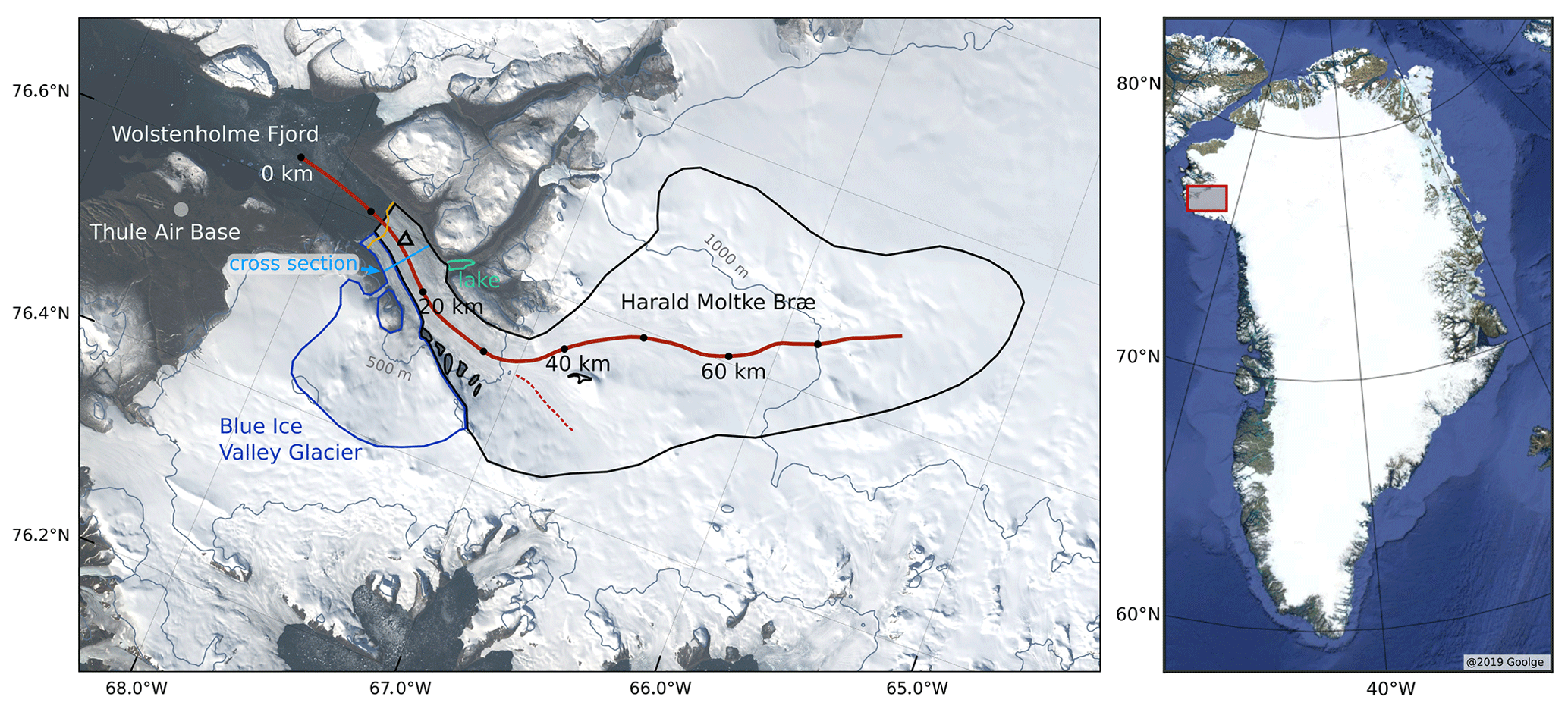
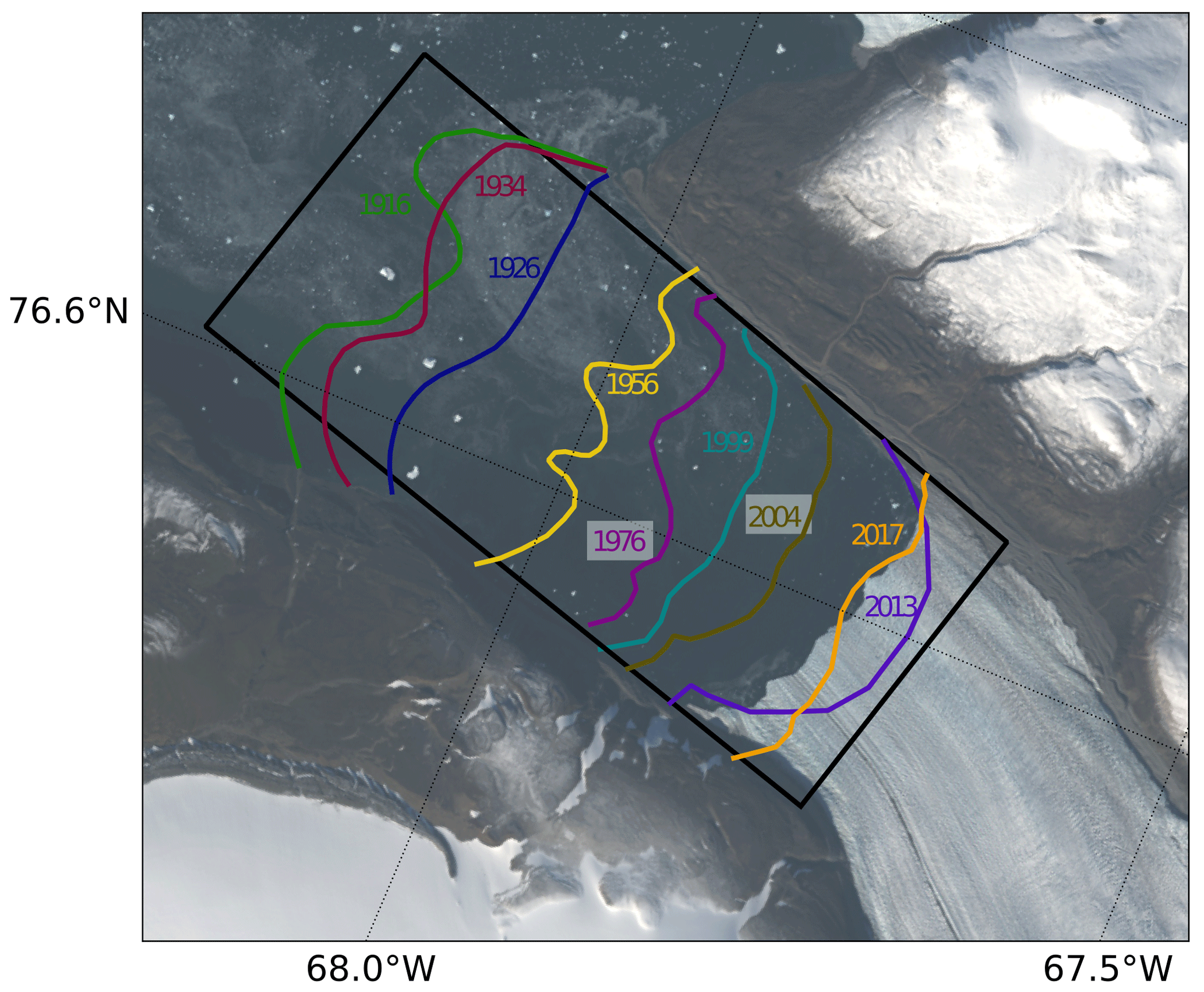
Figure 1 Region of investigation as viewed in a Landsat 8 scene of August 2014 (USGS, 2019) (see red box in the right image for its location in Greenland). Blue and black lines mark the drainage basins of Blue Ice Valley Glacier and Harald Moltke Bræ, respectively. Red lines (solid and dashed) mark the approximate centre line of the main glacier stream and of a tributary, respectively. The starting point of the centre line is at the mean position of the glacier front line in 1916 (year of the first available record of the front position). We use the glacier front position of 1916 as a reference for all longitudinal profiles and glacier front positions. The yellow line marks the approximate front positions of 2020. The black triangle marks the point (67.628^∘ W, 76.588^∘ N) to which all velocity time series in this paper refer.

3 Data and methods

3.1 Ice flow velocity data sets

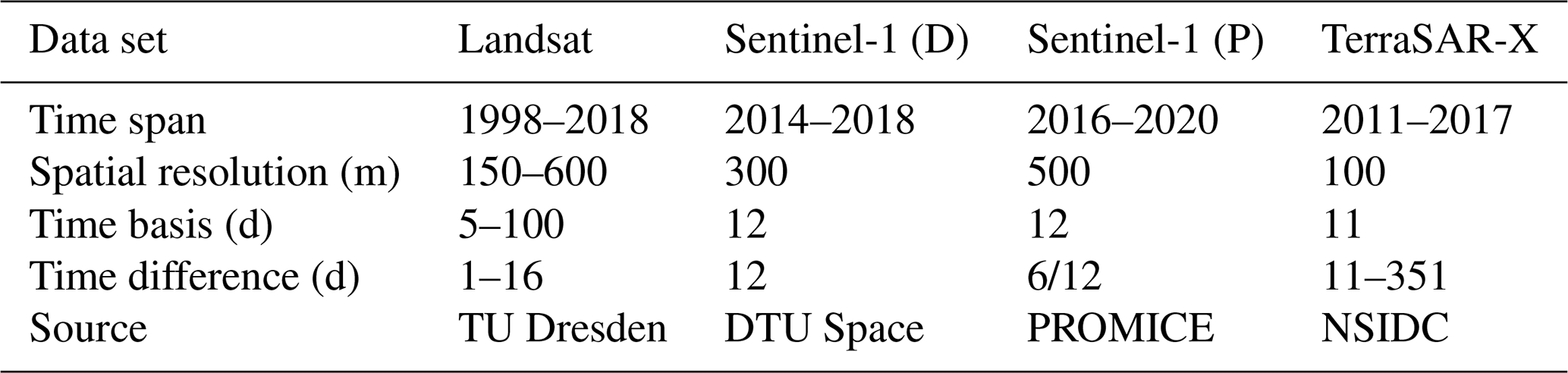
To determine flow velocity fields for outlet glaciers in Greenland, Rosenau et al. (2015) developed a processing scheme based on the feature tracking method using Landsat images available since 1972. Resulting velocity fields are used in the present study. In addition, we included three velocity data sets derived from synthetic aperture radar (SAR) offset tracking: Sentinel-1 (P) and Sentinel-1 (D) processed by PROMICE (Solgaard and Kusk, 2019) and DTU Space, respectively, and TerraSAR-X provided by MEaSUREs (Joughin et al., 2020). Table 1 provides technical details about these four data sets. Besides the time series comprising all available velocity data, we also use time series of monthly and semi-monthly averaged velocity fields for our analysis (Appendix A). By monthly and semi-monthly averaging of the velocity fields, a homogeneous and almost seamless time series can be inferred for the period after 2013. This is necessary for computing monthly ice-height change and ice flow rates. We assume that monthly and semi-monthly averaging is appropriate here, as the resulting time series still contain the main velocity variations (surges and seasonality) relevant for our study. Gaps in the Landsat data set caused by polar night are filled by data from SAR-based techniques. The accuracy of the joint velocity time series is shown to be better than 0.5 m d⁻¹ over most of the time but can exceed 1 m d⁻¹ in single months with rapidly changing ice flow (Appendix A). All velocity time series in this paper refer to the position indicated by the black triangle shown in Fig. 1. Based on the velocity fields and Landsat scenes, we chose a position that both experiences the largest velocity variations and remains behind the front throughout the study period.

Table 1 Overview of the technical details of the velocity data sets from Landsat, Sentinel-1 (D), Sentinel-1 (P) and TerraSAR-X. The velocity fields are given in the form of regular spatial grids. The time basis refers to the acquisition time difference of the image pairs used for the velocity determination. The time difference denotes the interval between two consecutive velocity fields.

3.2 Ice front position

For the period between 1916 and 1960, ice front positions are taken from the previous studies (Koch, 1928; Wright, 1939; Davies and Krinsley, 1962). For the period after 1972, ice front positions are digitized on the basis of Landsat images. The variation of the front position is measured by the average distance from its position in 1916 by applying a method proposed by Moon and Joughin (2008) (Appendix B).

3.3 Surface topography

We use three different digital elevation models (DEMs): ArcticDEM (June 2018) and two interferometric DEMs calculated from repeated TanDEM-X (TDM) acquisitions in January 2011 (7, 13, 18, and 24 January 2011) and December/January 2013/2014 (16 and 22 December 2013, 13 January 2014) (Krieger et al., 2020). The interferometric DEMs from TanDEM-X have been vertically co-registered over flat, ice-free terrain adjacent to Wolstenholme Fjord by adjusting their absolute phase offset (Krieger et al., 2020). Ice-surface height-change rates for the intermediate periods are obtained by computing the differences between these DEMs.

In addition to the measured surface elevation changes, we computed the monthly dynamic ice-height change rates to be expected due to the flow velocity distribution. This provides information on geometric glacier changes with a high sampling rate and enables a better understanding of how these changes are related to the flow velocity changes. To do so, we consider only the horizontal components of ice flow and assume parallel ice flow as well as a constant density of the glacier ice. Then, the relationship between ice flow and the dynamic height change at a given point is

$$\begin{array}{}\text{(1)}& {\displaystyle \frac{\partial H}{\partial t}}=-v\cdot {\displaystyle \frac{\partial H}{\partial x}}-H\cdot {\displaystyle \frac{\partial v}{\partial x}}.\end{array}$$

H denotes the glacier thickness, t denotes time, x denotes the position along the flow line and v is the depth-averaged velocity. We evaluate v by multiplying the observed surface velocities by a factor of 0.9 (Cuffey and Paterson, 2010; Wu and Jezek, 2004). This factor adopted in the absence of more specific information is a rough approximation and a potential source of error, particularly for surge-type glaciers. Note that the total surface height change is the sum of this dynamic height change and the height change due to surface mass balance (SMB).

We implement Eq. (1) by using velocity fields and ice thickness data (see the next section) interpolated to the main flow line. To suppress noise, we fit a straight line to the ice thickness profiles and a fourth-degree polynomial to the velocity profiles.

3.4 Bedrock topography

BedMachine v3 (Morlighem et al., 2017) provides both ocean floor and bedrock topography in a gridded format with a spatial resolution of 150 m. Additional bedrock data are available along profiles of airborne ground-penetrating radar measurements by the Center for Remote Sensing of Ice Sheets (CReSIS) from May 2014 and May 2015 (Paden et al., 2019). Based on a comparative analysis of BedMachine and CReSIS data (Sect. 3.7 and Appendix C), we use BedMachine data only for areas above 16 km of the centre line in Fig. 1.

3.5 Parameters of external forcing

The Regional Climate Model (RACMO2.3p2) provides the monthly cumulative surface mass balance (SMB), runoff, total melt (ice + snow) and precipitation at a resolution of 1 km (Noël, 2019). We average the SMB, precipitation and runoff over a fixed area, which is defined as the part of the glacier basin up-glacier of the cross section at about 16 km (Fig. 1). Additionally, we compute the ice-mass flux through this cross section. Therefore, we determine a cross-sectional profile of surface velocities scaled by a factor of 0.9. At each point of this profile, the mass flux through a vertical column in the glacier is computed using ArcticDEM and BedMachine. By summing up the resulting mass fluxes, we approximate the total flux through the cross-sectional area.

3.6 Visible features

We also assess changes traceable by visual inspection of the Landsat scenes. We focus on four different features: lakes on the glacier surface, outflow of subglacial meltwater at the glacier front (meltwater plumes), sea ice coverage in the fjord, and calving events (Appendix E). We assess these features by distinguishing between three states: not visible, moderate and strong occurrence.

4 Results

4.1 Flow velocity time series near the glacier front

Figure 2 shows the velocity variations in time, observed at a fixed position close to the terminus (Fig. 1). Ice flow accelerated significantly in 1999/2000 and 2005/2006 and in 2013–2019. During the 2013–2019 phase, the dense temporal sampling reveals pronounced seasonal velocity variations by 1 order of magnitude. At the end of 2019, velocities returned to a very low level that was sustained at least until July 2020.

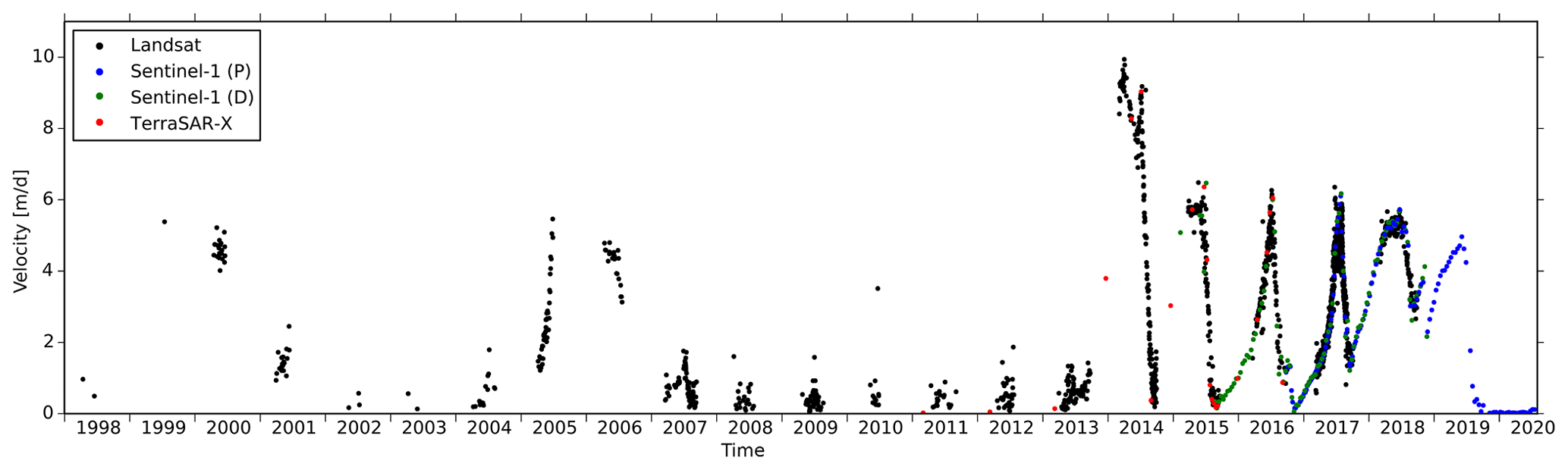
Figure 2 Flow velocity for the time period from January 1998 to July 2020 derived from Landsat, Sentinel-1, and TerraSAR-X at a point close to the terminus of Harald Moltke Bræ. For Sentinel-1 we use two different velocity data sets: one processed at Denmark's National Space Institute (DTU Space), referred to as Sentinel-1 (D), and another one provided by the Programme for Monitoring of the Greenland Ice Sheet (PROMICE), referred to as Sentinel-1 (P).

4.2 Front position

Figure 3 shows that most of the active phases between 1916 and 2020 were accompanied by an advance of the terminus which interrupted its long-term retreat (Mock, 1966). From 1926 to 1928 the frontal advance was more pronounced than in later active phases. During the surge event in 1954–1956, the glacier front retreated slightly.

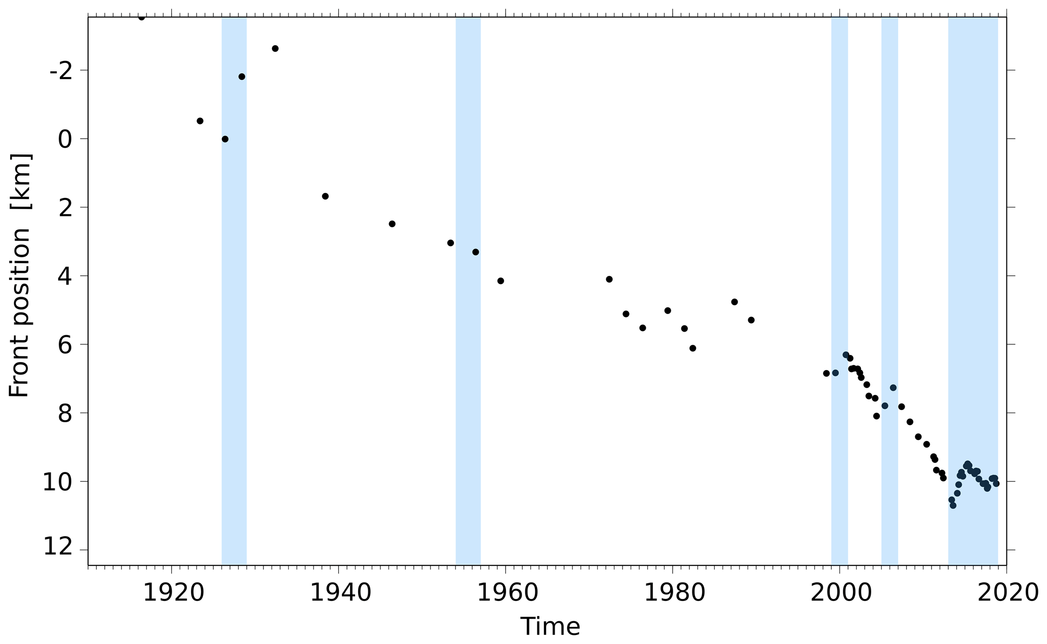
Figure 3 Average front position with respect to the terminus of 1916 consistent with the profile line shown in Fig. 1. The documented surges are marked by light blue colour.

Besides documented surge events, there are further phases of frontal advance between 1970 and 1985 for which, however, independent velocity observations are not available. Further, Fig. 3 indicates a long-term acceleration of the frontal retreat rate from about 100 m yr⁻¹ before 2000 to about 200 m yr⁻¹ thereafter (approx. 8 km between 1920 and 2000 compared to approx. 4 km between 2000 and 2020).

4.3 Ice flow during the active phases 1999/2000 and 2005/2006

In both active phases, 1999/2000 and 2005/2006, the glacier exhibits high velocities (>4 m d⁻¹) in late spring (Fig. 4). There is a rapid acceleration in spring 2005 and a rapid slowdown in summer 2006. In the years 2001, 2004 and 2007, which are before or after surge periods, an acceleration in spring and peak velocities in early summer are also visible. Over most of the rest of the quiescent phases the flow velocities remain clearly below 1 m d⁻¹ with no significant fluctuations.

Figure 4 (a) Yearly precipitation, meltwater runoff and SMB averaged over the drainage basin. (b) Monthly front position with respect to the year 1916 digitized in Landsat images where available. (c) Monthly glacier velocity and its uncertainty estimate derived from the Landsat data set at a point close to the terminus of Harald Moltke Bræ (black triangle in Fig. 1). The surges are marked by light blue colour.

During the quiescent phases the glacier front retreats (Figs. 3, 4), indicating that the flow velocity at the front is lower than the calving rate. In the years before the surge 2005/2006, this retreat was about 500 m yr⁻¹. In the active phases, the glacier front advances by about 500 m yr⁻¹, indicating that the flow velocity exceeds the calving rate.

Generally, no clear correlation between interannual variations of flow velocities and external influences (precipitation, runoff and SMB) could be identified (Fig. 4). Due to exceptionally high precipitation the SMB peaks in 2004 shortly before the initiation of the surge in spring 2005. The basin average annual SMB is negative after the termination of the surge in 2006 due to increased meltwater runoff. This implies that after 2006 the glacier loses mass even without ice discharge by calving.

The velocity fields visualized in Fig. 5 show that in both active phases, 1999/2000 and 2005/2006, the velocities were highest at the glacier front and decreased approximately linearly with increasing distance from the front. As indicated in Fig. 5c and d, shortly after the surge initiation (July 1999 and June 2005), fast ice flow is found, especially in the lower part of the glacier associated with steeply sloped velocity profiles. Towards the end of a surge (e.g. June 2000 and July 2006), however, upper parts of the glacier were increasingly affected by fast ice flow, whereas the velocities were decreasing close to the terminus.

Figure 5 Exemplary velocity fields (a, b) and velocity profiles (c, d) for the surges 1999/2000 and 2005/2006. The profile location is shown as a black line in (a), with black circles every 10 km along the profile. The starting point of this line is the glacier front position of 1916. The background image in (a, b) is a Landsat 8 scene (USGS, 2019).

4.4 Ice flow during the active phase 2013–2019

In autumn/winter 2013 there was an abrupt change from constantly low velocities of less than 1 m d⁻¹ in all months with available data to pronounced seasonal fluctuations over an order of magnitude with maximum velocities of 6–10 m d⁻¹ in spring and summer (Fig. 6). While the velocities dropped well below 1 m d⁻¹ in summers 2014, 2015 and 2016, they remained on a medium level above 1 m d⁻¹ in summers 2017 and 2018.

The front retreated by 1000 m yr⁻¹ between 2011 and 2013 (Fig. 6), faster than in the previous quiescent phases (500 m yr⁻¹), possibly due to a long-term increase in the calving rate. Due to this frontal retreat the constant point to which the velocities in Fig. 6 refer is located closer to the front in 2013. We note that this closer location to the glacier front could be one reason for the higher maximum velocity in 2013 compared to previous surges. However, it cannot be the main cause of the increase in flow velocities by 1 order of magnitude in 2013, since the acceleration in 2013/2014 affects the entire part between 13 and 25 km (Fig. 7). The high average velocity between 2013 and 2015 exceeded the calving rate and led to a rapid advance of the glacier front. Thereafter the terminus retreated on average by 200 m yr⁻¹, since the rather short-term accelerations in 2016 and 2017 were not sufficient to compensate for the calving rate.

Figure 6 (a) Yearly precipitation, meltwater runoff and SMB averaged over the drainage basin. (b) Monthly front position with respect to the year 1916 digitized in Landsat images where available. (c) Monthly glacier velocity and its uncertainty estimate derived from the Landsat data set at a point close to the terminus of Harald Moltke Bræ (black triangle in Fig. 1). Red error bars indicate the standard deviations of monthly velocity values from different data sets. The surges are marked by light blue colour.

The average SMB was exceptionally high (10 $\mathrm{kg}{\mathrm{m}}^{-\mathrm{2}}{\mathrm{d}}^{-\mathrm{1}}$) in 2013, the year of surge initiation. In contrast to the SMB maximum in 2004, the SMB maximum in 2013 is due to a low meltwater runoff rather than a high accumulation rate.

Figure 7 (a–d) Velocity fields for four selected months within the period from September 2013 to August 2014. The background image is a Landsat 8 scene (USGS, 2019). (e, f) Longitudinal and cross velocity profiles for the same year. Profile locations are shown in panel (a). The line marking the longitudinal profile location starts at the glacier front position of 1916 (same as in Fig. 5).

Directly before (September 2013) and after (August 2014) a phase of accelerated ice flow, the velocities were about 1 m d⁻¹ or less over almost the entire glacier (Fig. 7). A slight acceleration already occurred in July and August 2013 (Fig. 6). From September to December 2013 the velocities increased rapidly in the part below 20 km, whereas the parts further upstream were less affected or not affected at all. Subsequently, the upper parts of the glacier also accelerated significantly, leading to velocities of more than 5 m d⁻¹ within most of the glacier area below 25 km.

The longitudinal profiles in Fig. 7e show that a small part at the glacier front with an extension of 2–3 km had slightly increased velocities already in September 2013. Between April and July 2014, the ice flow was slowing down from month to month between 13 and 22 km, whereas it was continuing to accelerate further upstream. After the slowdown between July and August 2014, the glacier had the lowest velocities at the glacier front and a velocity maximum at about 29 km, unlike September 2013.

The cross velocity profiles in Fig. 7f show that both streams, the main stream of Harald Moltke Bræ and the part of Blue Ice Valley Glacier, were equally affected by the surge. Thus, the velocity changes had a uniform effect over almost the entire width of the glacier.

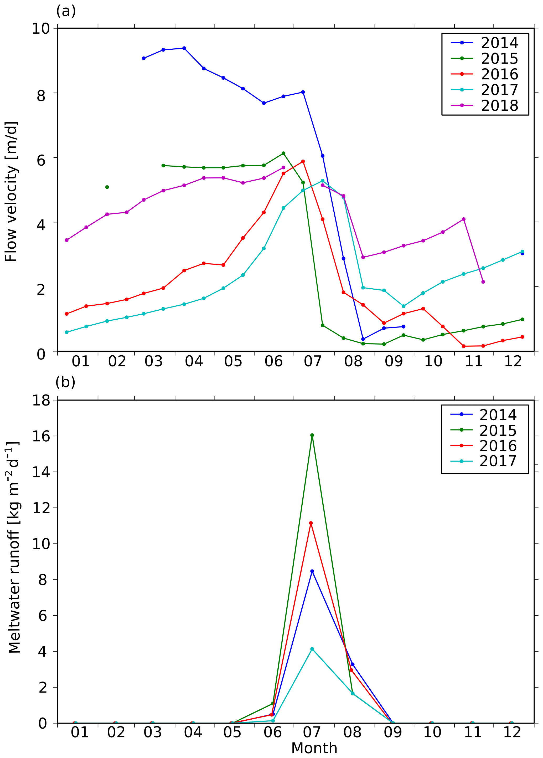
Figure 8 Seasonality of flow velocities (semi-monthly velocities at the point marked by the black triangle in Fig. 1) (a) and meltwater runoff (b). For 2018, data of meltwater runoff were not available.

Two distinct patterns of seasonal ice flow variations can be identified in Fig. 8a. In 2014, 2015 and 2018, the glacier reached high velocities of more than 4 m d⁻¹ already between January and March. By contrast, in 2016 and 2017, the velocities remained below 2 m d⁻¹ in autumn and increased only gently at the beginning of the year, followed by a rapid acceleration between May and June. The rapid slowdown in summer around July and August is common to all years between 2013 and 2018. These decelerations coincide with the maximum of the meltwater runoff (Fig. 8b).

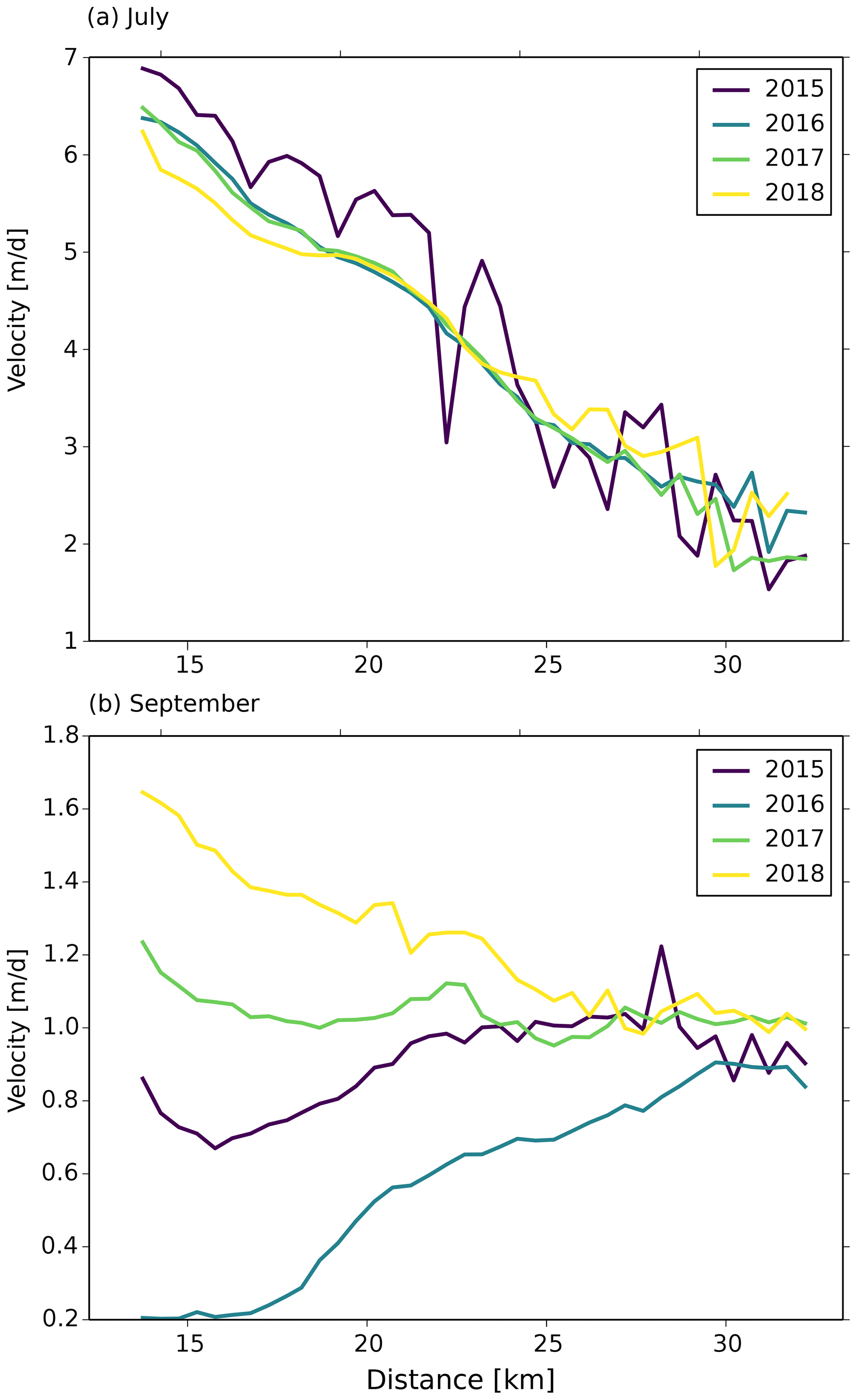
Figure 9 Longitudinal velocity profiles for always a month with high velocities (July) (a) and a month with low velocities (September) (b). The distance is measured from the 1916 glacier front position.

The longitudinal velocity profiles for July of the years 2015 to 2018 (Fig. 9a) all show a similar decrease from about 6.5 m d⁻¹ at 14 km to about 2 m d⁻¹ at 31 km.

In contrast to July, the profiles for September vary largely over the years 2015 to 2018 (Fig. 9b). In 2015 and 2016, velocities remained relatively low and had their maximum at approximately 29 km. In 2017 and 2018 (years with rapidly increasing velocities in autumn), velocities were highest at the glacier front. In 2015, 2016 and 2017, ice flow was enhanced within 2–3 km from the terminus.

4.5 Ice flow during the quiescent phases

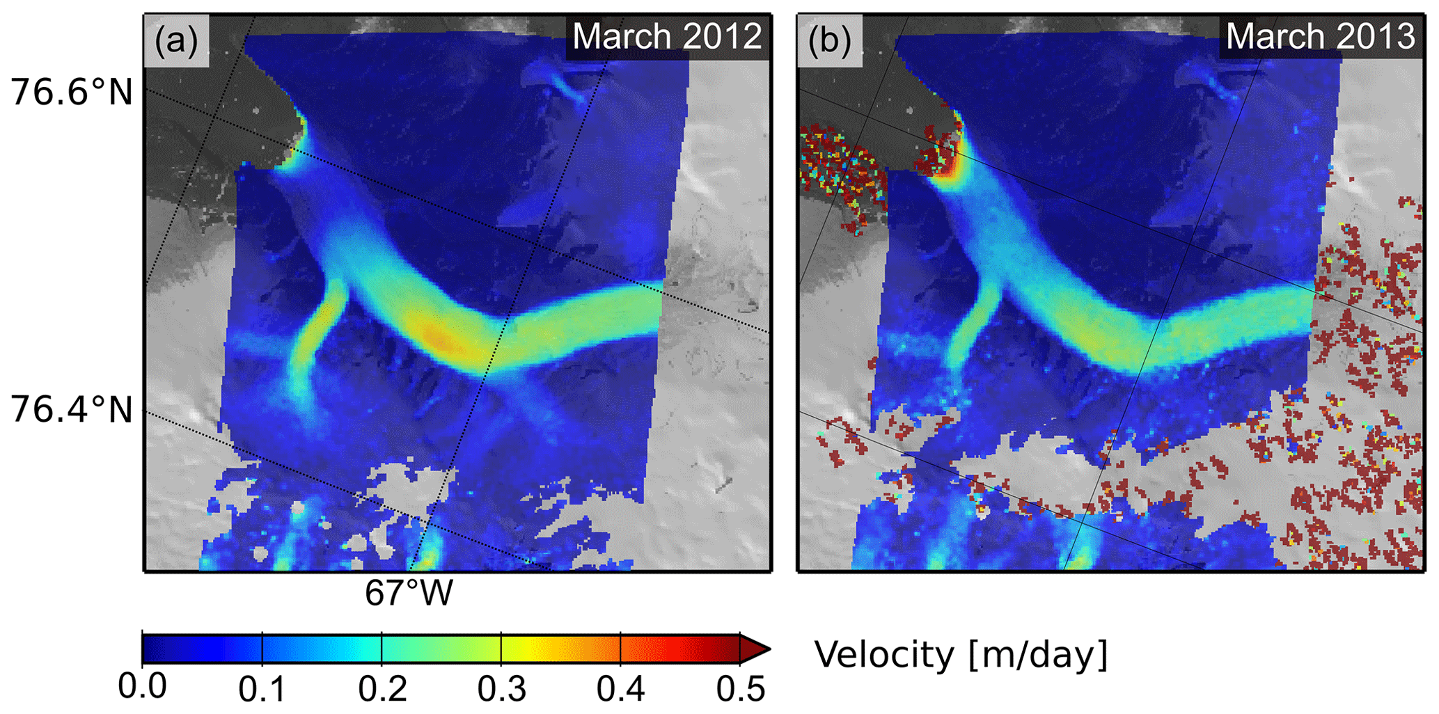
In the quiescent phase, velocity maxima amounted to 0.3–0.4 m d⁻¹ in both the main stream of Harald Moltke Bræ (about 29 km) and in the Blue Ice Valley Glacier about 2 km upstream from the confluence with Harald Moltke Bræ (Fig. 10). Velocities were lowest (lower than 0.2 m d⁻¹) within an area of about 8 km extent right below the confluence. Within 2–3 km from the terminus, however, velocities were slightly higher, at about 0.3 and 0.5 m d⁻¹ in March 2012 and March 2013, respectively.

Figure 10 Exemplary velocity fields during a quiescent phase in March 2012 and 2013. The background image is a Landsat 8 scene (USGS, 2019). The colour scale is different from that in the previous figures.

4.6 Visually inspected features

In years with high flow velocities (2014–2018), both calving events and the sea ice break-up in the fjord started earlier compared to the preceding quiescent phase (Fig. 11). Supraglacial lakes always formed in summer, followed by the formation of meltwater plumes at the glacier front. Meltwater plumes were larger in the active phase 2013–2019 than between 2011 and 2013. However, the extent of supraglacial lakes on the glacier surface was about the same before and after 2013. In contrast to the supraglacial lakes, the stationary lake at the northern side of the glacier does not exhibit any significant seasonal or long-term variations visible in the Landsat images.

Due to the low resolution of the Landsat images, the formation of crevasses was not analysed. All further remarks on crevasses are solely based on the assumption that the rapid velocity fluctuations involve crevasse formation.

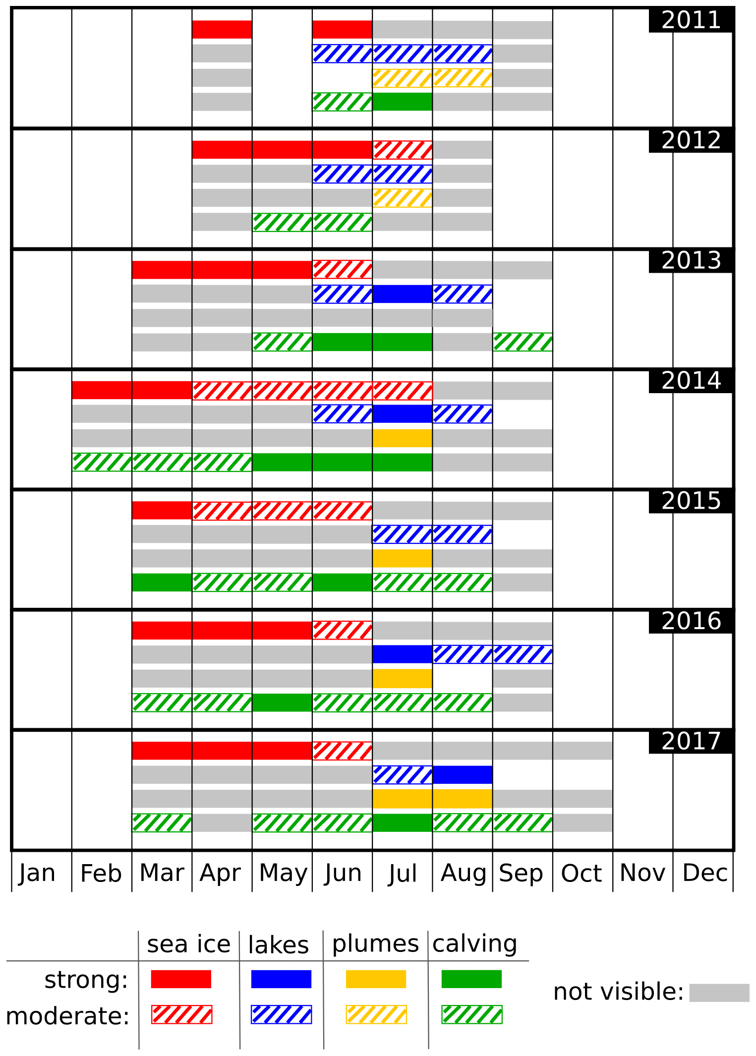
Figure 11 Occurrence of four different visual features from 2011 to 2017. Examples for the assessment of these visual features in Landsat scenes are given in Appendix E.

The middle moraine between Blue Ice Valley Glacier and the main stream of Harald Moltke Bræ, as inspected from the Landsat images, does not show any significant change in position or surge looped geometry (Appendix E), even during phases of highly variable flow velocities. This indicates that both glaciers were identically involved in the surge.

4.7 Ice-mass balance

The time series of the mass flow through a cross-sectional area close to the glacier front (Fig. 12) has three clear steps marking the surge events. During the surge phases, the estimated average ice-mass discharge was 0.5–1 Gt yr⁻¹ subject to uncertainties associated with the interpolation of flow velocities to unobserved months. During the quiescent phases, mass flux was mostly below 0.05 Gt yr⁻¹. The average SMB was roughly 0.2 Gt yr⁻¹ in 1990–1998 and 0.1 Gt yr⁻¹ in 2001–2004. Thus, between 1998 and 2006, the ice discharge exceeded SMB during the active phases, while SMB exceeded discharge during the quiescent phases. After 2006, however, both the ice flux and SMB contribute to an overall mass loss of about 0.4 Gt yr⁻¹. SMB maxima in 2004 and between autumn 2012 and spring 2014 precede the active phases 2005/2006 and 2013–2019.

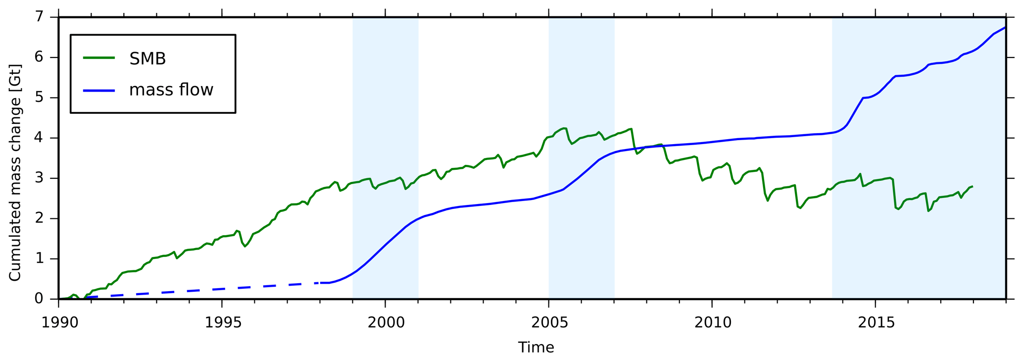
Figure 12 Cumulated mass flow through a cross section of Harald Moltke Bræ close to the terminus (blue) and monthly cumulated SMB (green) summed over the drainage basin. The surges are marked by light blue colour.

4.8 Bedrock and ice surface geometry

We examined the bedrock topography from BedMachine (Morlighem et al., 2017) and from CReSIS, both along the same CReSIS flight path (Fig. 13). BedMachine suggests a trough at 10–12 km (close to the front position of the year 2000) and a ridge at about 13 km (close to the front position in 2015) associated with an ice thickness as low as 40 m. The BedMachine uncertainty in this section is specified at a high level of 100 m. From 13 km up-glacier the BedMachine bedrock declines steeply to a depth of 200 m at 16 km with an uncertainty of 10–20 m (Morlighem et al., 2017). However, between 13 and 16 km, CReSIS data deviate significantly from BedMachine and suggest a gently sloped bedrock with a depth of about 230 m at the front position of the year 2015. From 16 to 25 km the BedMachine–CReSIS differences vary between 5 and 100 m, on the level of the uncertainties specified for BedMachine (Morlighem et al., 2017).

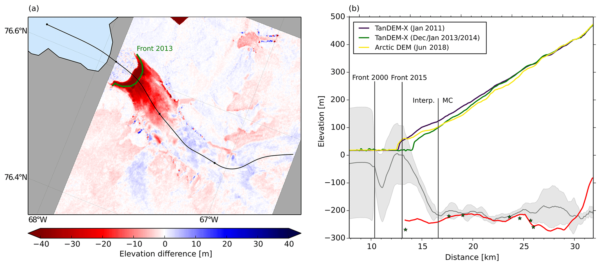
Figure 13 (a) Difference between ice surface elevations from two TanDEM-X observations (December/January 2013/2014 minus January 2011). (b) Profiles of bedrock topography from BedMachine (grey) and CReSIS (red) along the ground track of a flight path from May 2014 (Paden et al., 2019). Stated uncertainties for the BedMachine data set (Morlighem et al., 2017) are indicated by the grey error band. Green stars mark the elevations from independent CReSIS measurements at the intersections of the ground tracks. Vertical lines mark the front positions of 2000 and 2015 and the boundary between the areas where BedMachine applied interpolation and a mass conservation approach (MC), respectively (Morlighem et al., 2017). Profiles of glacier surface height at different times are also shown. Panel (a) also shows the profile location (black line starting at the glacier front position of 1916 and black circles every 10 km along the profile) and the front position of December/January 2013/14 (green line).

Below a distance of 16 km only interpolation methods were used in BedMachine (see Appendix C). Independent CReSIS observations are in good agreement with each other (see crossovers in Fig. 13). Thus, we assume that CReSIS provides a more accurate representation of the true bedrock topography close to the terminus and that the BedMachine sequence of a trough and a ridge at 10–12 and 13 km, respectively, are an interpolation artefact.

Surface elevations and elevation changes are also shown in Fig. 13. The difference between the 2013/2014 and 2011 TDM DEMs (Fig. 13a) reveals a significant ice thinning close to the glacier front by up to 30 m in the 3 years preceding the 2013–2019 surge, whereas parts further up-glacier at 30 km slightly thickened by an average of about 1–2 m. As a consequence, the glacier surface was steepening (Fig. 13b). Between 2013 and 2018, however, the glacier advanced and thickened in a small area at the terminus (Fig. 13b), so that there the surface slope became gentler again. Thus, the geometry near the glacier front in 2018 was similar to that in 2011. At the same time, the ice surface height between 17 and 24 km decreased from winter 2013/2014 to 2018.

Figure 14 Dynamically caused ice-height changes derived from velocity profiles along a flow line (as marked in Fig. 5). The distance is measured from the 1916 glacier front position.

Monthly profiles of dynamic ice-height changes along a flow line are shown in Fig. 14. During the quiescent phase before the surge initiation in 2013, the spatial distribution of flow velocities induced a rather slow dynamic thinning of the glacier tongue between 14 and 20 km and a slow thickening further up-glacier. The pattern of thinning near the terminus is amplified to values of up to 2 m per month in September 2013, shortly before the surge initiation. In December 2013 the extremum of surface lowering has moved further upstream (to 20 km) and has reached a value of −4 m per month. In spring 2014, the massive acceleration of the entire lower part of Harald Moltke Bræ up to 25 km entails a rapid dynamic increase in surface height (3–6 m per month) in the lowest 5 km of the glacier and a rapid thinning (−8 to −6 m per month) further up-glacier. During spring 2014 this pattern appears to propagate upstream.

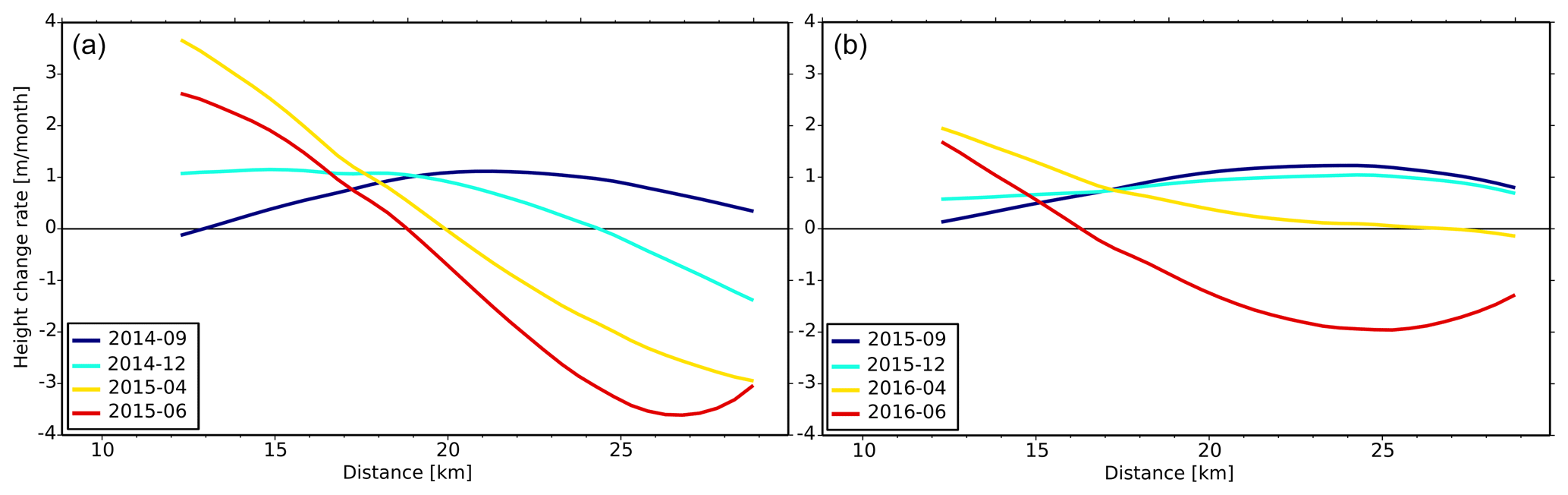
Figure 15 Dynamically caused ice-height changes derived from velocity profiles along a flow line for selected months during ice flow acceleration 2014/2015 (a) and 2015/2016 (b). The distance is measured from the 1916 glacier front position.

The accelerations of 2014/2015 and 2015/2016 (Fig. 15) differ from those of 2013/2014 as they were not preceded by a rapid thinning. The dynamic height changes in 2014/2015 and 2015/2016 indicate overall a simultaneous acceleration of the glacier rather than an up-glacier propagation.

5 Interpretation and discussion

The flow velocity variations of Harald Moltke Bræ exhibit at least two different signals: episodic surges and a seasonality with velocities abruptly decreasing in summer. For the identification of the surge periods, as mentioned in Sect. 1, we use both the strong change in flow velocity and the terminus advance as the main criteria (Sevestre and Benn, 2015). The occurrence of a pronounced seasonality in velocity simultaneously with a surge can be identified for the period 2013–2019 (Figs. 2 and 6). It would be conceivable that similar seasonal velocity changes were present during previous surges. In 1999, 2000 and 2005, any possible deceleration in July/August would have remained unobserved due to the lack of velocity data. In 2006 and 2007, flow velocities indeed decreased rapidly in summer, similarly to 2013–2019 (Figs. 4 and 6). Using the same data as the present study, yet at a different position, Rosenau (2014) showed that the velocities close to the terminus had decreased below 1 m d⁻¹ before they increased again in 2007. The rapid acceleration in spring 2005 and the velocity peaks in summers 2001, 2004 and 2007 are consistent with a seasonality that is characterized by maximum velocities in spring and early summer. Potentially, a seasonality of smaller amplitude was also present during the quiescent phases but could not be identified due to the limited accuracy of the Landsat velocity fields. Thus, our main hypothesis for the explanation of the surge behaviour of Harald Moltke Bræ is as follows: the effect of seasonally changing external influences on ice dynamics is episodically amplified due to internal feedback mechanisms.

5.1 Types of seasonal velocity variations

We distinguish three different types of seasonality (a)–(c) at Harald Moltke Bræ: (a) in some years (e.g. 2016 and 2017), there were low and rather gently increasing velocities at the beginning of the year, followed by a more pronounced acceleration from the onset of the melt season (Fig. 8). Despite a significantly lower amplitude, the seasonality of 2001, 2004 and 2007 may also be consistent with type (a). (b) In 2014 and 2015, for instance, the velocities were already high at the beginning of the year (as they increased in autumn of the previous year) and remained high over several months in spring (Fig. 8). In both cases (a) and (b), the flow velocities decrease rapidly in July or August. (c) During most of the quiescent phase, the velocities remained below 1 m d⁻¹. A significant variation in quiescent velocities cannot be detected either because it does not occur or because of the limited accuracy of the Landsat data.

5.2 Seasonal mechanism

Type-(a) and -(b) behaviours correspond to the seasonality of the glacier types (2) and (3), respectively, identified by Moon et al. (2014) and Vijay et al. (2019) (Sect. 1). Harald Moltke Bræ switches between type-2 and type-3 behaviours. Further, during the surges, the seasonal variations being about 6 m d⁻¹ clearly exceed the fluctuations of about 1–2 m d⁻¹ observed by Moon et al. (2014).

The deceleration of type-2/3 glaciers during the late melt season is correlated with the maximum of meltwater runoff, indicating a transition from an inefficient to a channelized drainage system (Moon et al., 2014; Vijay et al., 2019). Similarly to that, there may be a transition from an inefficient to an efficient subglacial drainage system in July/August in years with a seasonality of our type (a) or (b).

Some additional observations indicate a hydrological control on the seasonality at Harald Moltke Bræ: the formation of large supraglacial meltwater lakes at the beginning of the summer when velocities are highest (see the example in Appendix E), the occurrence of a meltwater plume shortly thereafter, the speedup at the onset of the melt season, and, further, the short-lived accelerations of ice flow right before the slowdown in 2014 and 2015 as a presumed effect of enhanced basal water pressure which subsequently leads to the formation of an efficient drainage system.

According to Moon et al. (2014), type (3) differs from (2) in autumn as there is still enough meltwater available to raise the water pressure significantly and, thus, to accelerate the ice flow. At Harald Moltke Bræ, we find a rather converse relationship: compared to years with low meltwater runoff (e.g. 2017), in years with larger meltwater runoff the ice flow slows down a bit earlier (already in July instead of August), the velocities decrease to a lower level and the deceleration is not directly followed by a rapid velocity increase in autumn (leading to type a in the following year) (Fig. 8). Potentially, more meltwater leads to a more efficient subglacial drainage system that prevails for a longer time in the year so that less meltwater is trapped at the glacier base in autumn. Consequently, the comparably less pronounced decelerations in 2017 and 2018 may be interpreted as an effect of lesser amounts of meltwater runoff.

5.3 Is the surge 2013–2019 different from previous surges?

There are several similarities between the surges 1999/2000 and 2005/2006: a duration of 2 years (years with velocities exceeding 4 m d⁻¹), persisting high velocities over at least 3 months in the second year of the surge (2000 and 2006) (Fig. 5), and a year with slightly enhanced summer velocities following the surge. By contrast, the surge 2013–2019 had at least 6 years with velocities exceeding 4 m d⁻¹. Further, the surge 2013–2019 was initiated by an abrupt acceleration in autumn/winter reaching velocities of up to 10 m d⁻¹, whereas the surge 2005/2006 began with an acceleration in spring 2005. It is likely that all three observed surges, 1999/2000, 2005/2006 and 2013–2019, were modulated by a similar mechanism of seasonality.

It must be considered that – before 2013 – the flow variability may be underestimated due to data gaps and larger time bases (Appendix A) which involve large smoothing effects. Due to the retreat of the glacier front, the fixed reference point for the velocities was closer to the glacier front in 2013 than at the times of previous surges. This is likely one reason why velocity peaks in 2013 to 2019 are higher than during previous surges. Thus, the surges 1999/2000, 2005/2006 and 2013–2019 might be more similar than suggested at first glance in Figs. 2 and 6. However, in terms of its duration, the most recent surge clearly differs from the surges 1999/2000 and 2005/2006.

As the observed accelerations 1926–1928 and 1954–1956 refer to the average over a period of 2 years, the true maximum velocities are probably significantly higher than the documented velocities of 3.6 and 1 m d⁻¹, respectively. In addition, the exact timing of the surges is unknown. They may have lasted longer or shorter than 2 years. In summary, there are not enough data to state whether the surges 1926–1928 and 1954–1956 were significantly different from the more recent surges.

5.4 Classification of flow patterns

We distinguish between four different flow patterns (A–D) based on the spatial distribution of flow velocities. Each pattern is associated with a certain profile of dynamic ice-height changes and, thus, has certain consequences for the stresses and the mass redistribution in the glacier system.

(A) A first pattern is characterized by low velocities (<0.3 m d⁻¹) in the lower part of the glacier and moderately higher velocities further upstream. This causes only minor dynamically induced changes in the receiving area and a dynamic thickening in the reservoir area (Fig. 16). This pattern can be found for many of the quiescent phases, e.g. in March 2012 (Fig. 10a). In pattern (B), the glacier exhibits low flow velocities (<0.5 m d⁻¹) over most of its area except for a small part at the front where the velocities exceed 1 m d⁻¹ (Fig. 16). This pattern arises shortly before the surge initiation, e.g. in September 2013 (Fig. 7). Thus, a pronounced thinning occurs directly at the glacier front. (C) A third pattern has a steeply sloped velocity profile (with a maximum of about 6–10 m d⁻¹ at the glacier front) in the lower 10 km of the glacier, whereas larger parts further upstream remain at low velocities similar to patterns (A) and (B) (Fig. 16). This was the case in December 2013 (Fig. 7), for instance. This pattern may be associated with only moderate height changes at the glacier front and in the upper parts of the glacier, whereas the middle part of the glacier is rapidly thinning (Figs. 14 and 16). This results in a decrease in surface slope at the terminus and a significant increase in surface slope in the middle part. (D) The fourth pattern shows high velocities at the glacier front, similar to pattern (C). (D) differs from (C) in that it has higher velocities in the middle and upper parts of the glacier (Fig. 16). This is associated with a more gently sloped velocity profile in the lower 10 km of the glacier. As a consequence, the glacier is dynamically thickening in its lower part and thinning in its upper part. Pattern (D) reverses the combined effect of patterns (A) and (B), however, with a difference in magnitude. Thus, the effect of the longer-lasting quiescent phase can be compensated for by a shorter-lasting active phase. Pattern (D) can be found e.g. in the velocities of spring and early summer 2014 (Fig. 7).

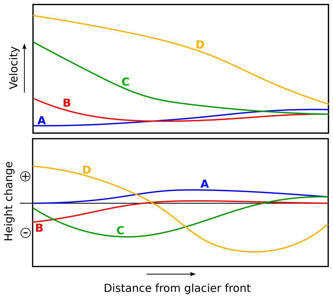
Figure 16 Schematic representation of the velocity and the corresponding dynamic ice-height changes for the patterns (A), (B), (C) and (D).

During the initiation of the surge 2013–2014, these flow patterns followed each other in the sequence (A)–(B)–(C)–(D). Similarly to winter 2013/2014, the velocity profiles in 1999 and 2005 (first year of the surge) were also steeper than in the following years 2000 and 2006 (second year of the surge). Hence, there might have been a similar sequence (A)–(B)–(C)–(D) initiating all surges. This sequence reflects an evolution of dynamic changes within the glacier where first, through pattern (B), mass from the middle part of the glacier is mobilized to compensate for the mass deficit at the glacier front leading to (C). Subsequently, the surplus of mass in the upper part of the glacier is set in motion to compensate for the mass deficit in both the middle and lower parts, resulting in pattern (D).

In the years after the surge initiation, the sequence appears to be different. There is a rather direct switch between (A) and (D), whereas the patterns (B) and (C) are largely absent (Fig. 15).

5.5 Up-glacier propagation of the surges

The sequence of patterns (A)–(B)–(C)–(D) is consistent with an up-glacier propagation of the surge. In the consecutive years, however, the direct switch between (A) and (D) reflects a rather uniform acceleration of most of the ablation zone of Harald Moltke Bræ. Based on these findings, we conclude that once the entire glacier has accelerated, large parts of the glacier are set into a condition to accelerate again in the following years.

5.6 Glacier geometry during the quiescent phases

Similarly to other surge-type glaciers, the quiescent phase of Harald Moltke Bræ is characterized by slower flow in the lower part and faster flow in the upper part. However, the transition between slower and faster flow is rather smooth, which implies just a slight dynamic thickening (a few metres over 3 years; see Fig. 13). We therefore hypothesize that for the initiation of the surge, the increase in driving stresses in this transition zone is less important than the decrease in resisting stress at the glacier front implied by the frontal retreat. The findings are opposite to down-glacier propagating surges e.g. observed at Variegated Glacier (Raymond, 1987) and at Bivachny Glacier (Wendt et al., 2017). The pronounced thinning at the glacier front is compatible with an up-glacier propagating surge observed at Aventsmarksbrae (Sevestre et al., 2018). Thus, a significantly larger thinning at the glacier front compared to a lesser thickening in the upper part of the glacier could be a key factor for the surge initiation at the terminus and an up-glacier propagation.

5.7 Potential causes and triggers of the surges

On long timescales, the dynamics of Harald Moltke Bræ may be determined by externally driven influences such as SMB and the long-term retreat of the glacier front. On the interannual timescale, however, the flow velocity does not react simultaneously to external drivers such as the terminus retreat and the cumulated SMB. Instead, local conditions might restrict the ice flow during the quiescent phase and facilitate an increasing instability that finally results in a surge.

Several factors may potentially restrict the ice flow in the lower part of the glacier during a quiescent phase: a cold glacier base that is partly frozen to the glacier bed (corresponding to the thermally driven mechanism, maybe related to strengthened subglacial till), a subglacial drainage system remaining efficient over several years (corresponding to the hydrologically driven mechanism), a bump in the bedrock topography, a dynamic interaction of Blue Ice Valley Glacier and Harald Moltke Bræ, and the absence, or closure, of crevasses preventing meltwater from reaching the glacier base.

Wendt et al. (2017) discussed a bump in the glacier bed as the cause of restricted ice flow during the quiescent phase of Bivachny Glacier. At Harald Moltke Bræ, there is a bump at about 25 km according to the CReSIS data set, which is, however, small compared to the ice thickness. Closer to the terminus, the large uncertainties of the BedMachine data set do not allow us to identify relevant features of the bedrock topography.

The presence of a seasonality parallel to surges has been taken as a clear indicator of a hydrologically driven mechanism at other glaciers (Wendt et al., 2017; Raymond, 1987). Furthermore, the rapid onset of the surge in 2013 suggests a hydrological mechanism. By contrast, a thermally driven mechanism is typically characterized by a rather gradual surge initiation (Murray et al., 2003; Jiskoot, 2011). A thermally driven mechanism is also unlikely, as the intermediate decelerations during summer, when the glacier goes back to a state similar to the quiescent phase, cannot be explained by an abrupt freezing of the glacier base or a strengthening of subglacial sediments. Therefore, the hydrologically driven mechanism provides an overall more plausible explanation for the surges at Harald Moltke Bræ than a thermally driven mechanism.

The surges of Harald Moltke Bræ may develop as follows: during the quiescent phase, the combined effect of low flow velocities and a negative mass balance in the ablation zone involves a thinning and steepening of the glacier tongue and a retreat of the glacier front. Observations from CReSIS indicate a rather thick marine-terminating glacier front of more than 200 m which could facilitate the thinning and the retreat. These factors may lead to a decrease in resisting forces at the terminus. Additionally, at a thick glacier, the steepening of the glacier due to thinning at the terminus could increase the driving stress (Sevestre et al., 2018). The resulting large net stress in the flow direction may cause a small area at the glacier front to accelerate (flow pattern B). This induces different effects that facilitate a further acceleration and the upward propagation of the surge: crevassing of the ice surface enabling more meltwater to reach the glacier base (Sevestre et al., 2018), weakening of subglacial till (deformation of the glacier bed), longitudinal stresses (tension) and a further surface thinning/steepening. As a result, the glacier may change into pattern (C), which, in turn, transfers these processes further up-glacier, leading to pattern (D). Once the entire ablation zone of Harald Moltke Bræ was affected by the sequence (A)–(B)–(C)–(D), the externally driven seasonal changes in meltwater availability could have a more pronounced effect as crevasses have spread over large parts of the glacier and subglacial till has weakened.

This could explain why in years after the year of surge initiation there is a simultaneous acceleration of large parts of the glacier according to a direct flipping between (A) and (D) rather than an up-glacier propagation. Pattern (D) causes the ice surface to become more gently sloped. Such a decrease in surface slope could stabilize the glacier during the surge and, thus, lead to a reverse feedback: a decreasing annual amplitude causing a gradual closure of the crevasses and, possibly, a strengthening of the subglacial sediments until the glacier enters a quiescent phase. Such an evolution is consistent with the velocity peaks in summer 2001 and 2007 following the surges.

Both the SMB and the retreat of the glacier front could determine the time of initiation and the length of the surge cycle. The 2013–2019 surge and its preceding quiescent phase lasted longer (5 and 6 years) than the surge and the quiescent phase in the preceding cycle (5 and 2 years, respectively). This could be related to the SMB in the drainage basin being negative after 2006. Also, the intermediate annual retreat of the glacier front in 2016 and 2017 could have prevented the glacier from stabilizing such that in 2018 and 2019 velocities of more than 4 m d⁻¹ are still reached.

6 Conclusions

By combining four different remotely sensed velocity data sets, we estimated a monthly velocity time series for Harald Moltke Bræ with high spatial and temporal resolution. Based on this time series we identified mainly two different signals of velocity variations close to the terminus of Harald Moltke Bræ: episodic surges and a pronounced seasonality. As we assume that there is a similar seasonality in most years of the observation period, we interpret the surges as phases with a strongly amplified seasonal amplitude.

The annual flow velocities of Harald Moltke Bræ were high over a relatively long period of 6 years from 2013 to 2019, which has not been observed in this way before. However, flow velocities remaining low in autumn/winter 2019 and spring 2020 indicate the beginning of a new quiescent phase. Thus, the high velocities between 2013 and 2019 may constitute a longer surge than previous ones but no fundamental change in the flow regime. We therefore assume that Harald Moltke Bræ is likely to maintain its surge behaviour.

Regarding temporal velocity variability, we identified types of seasonality which indicate a hydrological control of the seasonal velocity changes. The time of a rapid deceleration in July or August suggests a switch between an inefficient and an efficient subglacial drainage system due to the changing amount of meltwater availability. This, however, does not provide an explanation for the significant increase in seasonal amplitude during the surges.

Over the past 2 decades, the overall discharge of the glacier was larger than the overall ice mass accumulation. Thus, the overall thickness of the glacier was decreasing, which could be a reaction to the observed long-term retreat of Harald Moltke Bræ. However, the glacier does not react instantaneously to the terminus retreat by dynamic thinning. The reason might be a restricted ice flow during the quiescent phases due to internal factors, probably related to the glacial hydrology. This possibly causes an increasing instability and results in an alternation of two reverse feedback mechanisms which involve pronounced acceleration and deceleration, respectively.

By distinguishing between different patterns of spatial distribution of flow velocities, we could demonstrate that the surge develops first at the glacier front and that it is propagating rapidly up-glacier within a few months thereafter. The seasonal amplitude remains high in the years after the year of surge initiation, with a rather simultaneous acceleration of the entire ablation zone of Harald Moltke Bræ. Thus, we assume that during the surge there are favourable conditions for an enhanced effect of the seasonally changing meltwater availability on the ice flow. This could be a crevassed glacier surface and possibly weakened subglacial till. As the seasonal amplitude decreases gradually after the surges, there might be a stabilization related to the flattening of the glacier with increasing duration of the surge.

The presence of additional factors that could restrict ice flow during the quiescent phase such as a bump in the bedrock topography or a reversely sloped bed at the terminus could not be identified. However, the stationary lake at the northern side of Harald Moltke Bræ and the confluence between the Blue Ice Valley Glacier and Harald Moltke Bræ could be factors that facilitate the surge behaviour.

External factors may not be the cause of the surge behaviour but could play an important role for the time of the initiation and the duration of the surges. Particularly, the rapid retreat of the glacier front with an acceleration and a thinning of a small area at the terminus during the quiescent phase may determine the way in which the surges develop. The marine-terminating glacier front could, thus, be an important factor for the surge behaviour of Harald Moltke Bræ.

Appendix A: Velocity data sets and determination of joint velocity time series

A1 Initial velocity fields and pre-refinements

The velocities derived from remote sensing techniques represent average values over the given time basis, the time basis being the time difference between the acquisition epochs of the two images used for the velocity estimation. Thus, long time bases might result in a stronger temporal smoothing. Regarding the quality and the temporal coverage of the Landsat velocity fields, the deployment of the Operational Land Imager (OLI) at Landsat 8 launched in 2013 was a significant improvement. It extended the yearly image acquisition to the period March–November, while the acquisition period was May–October before Landsat 8. It also improved the spatial resolution of the derived velocity fields from 300 to 150 m. These improvements, in turn, enabled us to use image pairs with shorter time bases and, thus, the resolution of rather short-term velocity fluctuations. The initial Landsat data set contains velocity fields with very different time bases (Table 1), which leads to varying smoothing effects (Fig. A1).

Therefore, we reject those velocity fields with a time basis longer than 60 d in order to avoid strong smoothing effects. Further, we do not use Landsat ice flow velocity fields with a time basis shorter than 25 d, as these are assumed to be of comparatively lower accuracy.

Velocities are analysed in the form of spatial fields, time series with respect to a point close to the glacier front or velocity profiles along a flow line.

A2 Estimation of monthly velocity fields

To ensure consistency when determining a joint time series, all given data grids are transformed to the coordinate system of the Landsat data (Polar Stereographic Grid North). Subsequently, monthly medians are calculated separately for each data set. The resulting monthly time series are merged by computing the monthly mean for each cell. A similar approach was applied to determine semi-monthly velocity fields.

Table A1 First row: uncertainties specified for each data set. Rows 2–4: root-mean-square (RMS) differences between the two data sets indicated in the line and column heads, evaluated within the ablation area of Harald Moltke Bræ. As the temporal variability of the flow velocities within 1 month is not negligible, we distinguish between months with slow maximum velocities (<2 m d⁻¹) and high maximum velocities (>5 m d⁻¹, parentheses). Unit is m d⁻¹.

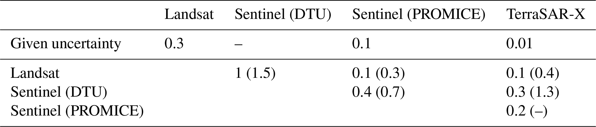
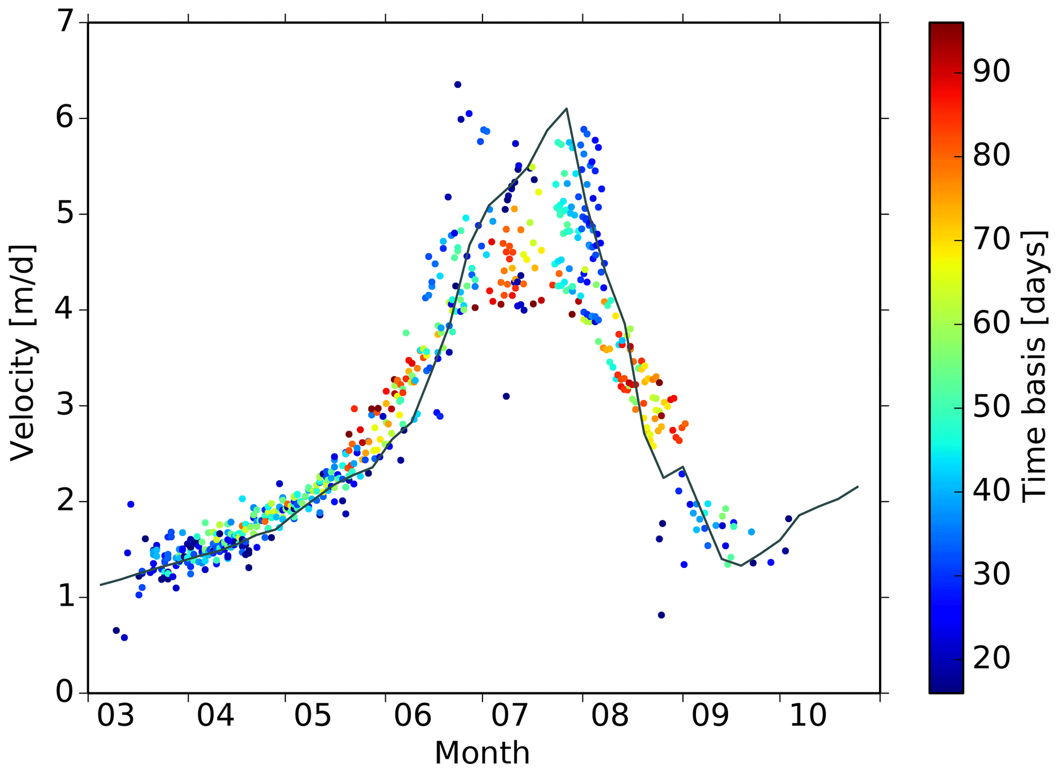
Figure A1 Landsat velocities at the terminus of Harald Moltke Bræ in the year 2017, colour scaled with the time basis. For comparison, the velocities from Sentinel-1 (P) are plotted as grey line.

A3 Accuracy of the velocity fields

The point velocities derived from different methods (Fig. 2) agree well, with only minor deviations being generally less than 0.5 m d⁻¹. The uncertainties specified for Sentinel-1 (P) and TerraSAR-X (0.1 and 0.01 m d⁻¹, respectively) are significantly lower than the uncertainties for Landsat (0.3 m d⁻¹, Table A1). However, methods applied for uncertainty assessment may differ between the data sets. A direct comparison of the monthly medians shows that the mean deviations between Landsat, Sentinel-1(P) and TerraSAR in the ablation zone of Harald Moltke Bræ range from 0.1 to 0.4 m d⁻¹ in phases with low velocities (<2 m d⁻¹) and from 0.3 to 1.3 m d⁻¹ in phases with high velocities (>5 m d⁻¹). We conclude that the accuracy of the estimated joint time series of monthly velocities significantly depends on the magnitude and the temporal variability of the flow velocities.

Appendix B: Ice front positions

To compute the mean ice front position change, we define a rectangle approximately having the width of the glacier as shown in Fig. B1 (Moon and Joughin, 2008). The glacial area enclosed by the front positions and the rectangle is determined and divided by the width of the rectangle to obtain the average change in the front position.

Figure B1 Digitized ice front positions and rectangle used for the estimation of the mean front position change. Background image: Landsat 8 scene of 2014 (USGS, 2019).

Appendix C: Bedrock geometry

As shown in Fig. 13, the BedMachine bedrock topography exhibits a significant depression close to the front position of the year 2000 (terminus position used in BedMachine), a pronounced elevation at the terminus position of 2015 and a sharply down-sloping bedrock further upstream. The methods applied for bedrock topography determination depend on surface properties and data availability (Morlighem et al., 2017). The mentioned distinct topographic features coincide with transitions between different methods and different associated uncertainty levels (Fig. C1a, c). In particular, different interpolation methods prevail near the glacier front. A synthetic approach was applied for Wolstenholme Fjord (Williams et al., 2017), where only few bathymetry data were available. There, the assessed uncertainties are as large as 250 m (Morlighem et al., 2017).

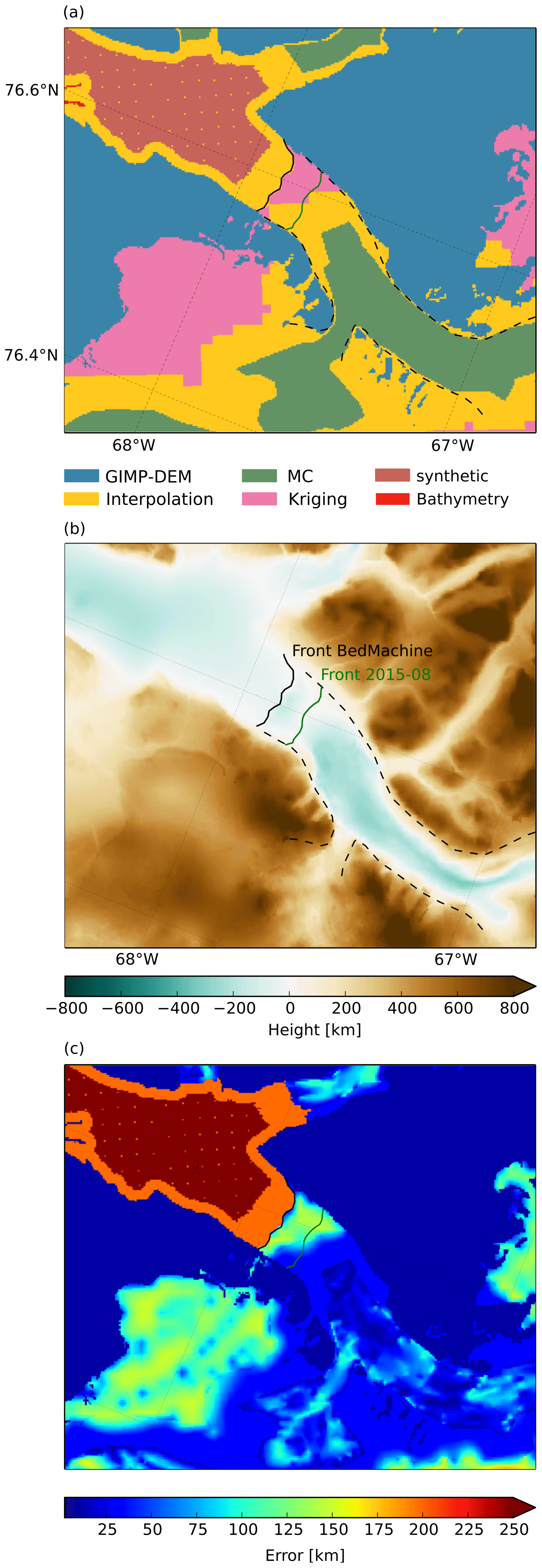
Figure C1 Comparison of the applied methods, the resulting bedrock topography and the corresponding error estimations by Morlighem et al. (2017). Elevations are given with respect to the WGS84 ellipsoid.

Appendix D: Dynamic ice-height change

To determine the dynamic ice-height change using Eq. (1), profiles of ice thickness and velocity are used. The ice thickness for the dynamic height change estimation is approximated by the difference between the ice surface elevation from ArcticDEM and the bedrock topography. Test results for the dynamic height changes have been computed with the bedrock topography from CReSIS and from BedMachine for distances >16 km along the profile. The results showed approximately the same overall pattern of dynamic height changes as when using a constant height of −250 m. The steeply sloping profile from BedMachine is assumed to be an artefact due to interpolation methods. Minor structures (<20 m) in the bedrock topography can be neglected for their small effect on the derived patterns of dynamic ice-height changes. Thus, we used a constant bedrock topography of −250 m to compute rough patterns of dynamic height changes.

Appendix E: Visually inspected features in Landsat images

Figure E1a shows Harald Moltke Bræ at the time with high flow velocities shortly before the deceleration. This scene is an example of the strong occurrence of supraglacial meltwater lakes and iceberg calving. As sea ice is still present but has already broken up, we assess the occurrence of sea ice here as moderate. Due to ice mélange the presence of a meltwater plume cannot be evaluated in this scene. Figure E1b shows the glacier during the rapid slowdown. In this scene, calving is no longer visible. Sea ice and supraglacial lakes are only moderately present. A strong meltwater plume can be detected at the glacier front. In Fig. E1b, which shows Harald Moltke Bræ after the deceleration, none of the four features is visible. In Fig. 11, we assess the state of these features on a monthly basis. For this, we use multiple scenes per month and choose the state that is predominant during the month.

Figure E1 Exemplary three different Landsat scenes during the phase of highly variable flow velocities in summer 2014 (USGS, 2019).