the Creative Commons Attribution 4.0 License.
the Creative Commons Attribution 4.0 License.
 | 12 Jul 2021
Presentation and evaluation of the Arctic sea ice forecasting system neXtSIM-F
Timothy Williams
Anton Korosov
Pierre Rampal
Einar Ólason
The neXtSIM-F (neXtSIM forecast) forecasting system consists of a stand-alone sea ice model, neXtSIM (neXt-generation Sea Ice Model), forced by the TOPAZ ocean forecast and the ECMWF atmospheric forecast, combined with daily data assimilation of sea ice concentration. It uses the novel brittle Bingham–Maxwell (BBM) sea ice rheology, making it the first forecast based on a continuum model not to use the viscous–plastic (VP) rheology. It was tested in the Arctic for the time period November 2018–June 2020 and was found to perform well, although there are some shortcomings. Despite drift not being assimilated in our system, the sea ice drift is good throughout the year, being relatively unbiased, even for longer lead times like 5 d. The RMSE in speed and the total RMSE are also good for the first 3 or so days, although they both increase steadily with lead time. The thickness distribution is relatively good, although there are some regions that experience excessive thickening with negative implications for the summertime sea ice extent, particularly in the Greenland Sea.
The neXtSIM-F forecasting system assimilates OSI SAF sea ice concentration products (both SSMIS and AMSR2) by modifying the initial conditions daily and adding a compensating heat flux to prevent removed ice growing back too quickly. The assimilation greatly improves the sea ice extent for the forecast duration.
- Article
(3294 KB) - Full-text XML
- BibTeX
- EndNote


Arctic sea ice has been in great decline in the last number of years (Meier, 2017). Perovich et al. (2018) report that in 2018, the summer extent was the sixth lowest and the winter extent was the second lowest in the satellite record (1979–2018). Moreover, surface air temperatures in the Arctic continued to warm at twice the rate relative to the rest of the globe, and Arctic air temperatures for the past 5 years (2014–2018) have exceeded all previous records since 1900 (Overland et al., 2018), which will also contribute to future sea ice decline if it continues.
With less sea ice comes an increase in summertime accessibility for shipping. Azzara et al. (2015) considered a range of different scenarios and projected an increase in the number of vessels operating in the Bering Strait and the US Arctic of between 100 and 500 %. The International Maritime Organization has also recognised that shipping would increase and adopted an International Code for Ships Operating in Polar Waters (Polar Code)1 on 1 January 2017. This polar code addresses the increased safety and pollution risks of operating in the Arctic. A recent example of the risks and concomitant costs of accidents in the Arctic is the rescue of the fishing vessel Northguider, which ran aground between Spitzbergen and Nordaustlandet (Svalbard) after getting into trouble with sea ice. The crew had to be rescued by the Norwegian Coast Guard icebreaker KV Svalbard, who then had to drain 300 kL of diesel from the damaged vessel.2
Thus sea ice forecasting is becoming increasingly important. As well as search and rescue/accident prevention, other applications are optimised ship (icebreaker) routing based on forecasts (Kaleschke et al., 2016) and support of research activities – e.g. Schweiger and Zhang (2015) give an example of scheduling of high-resolution synthetic-aperture radar (SAR) images in order to follow the drift of some ice-mass balance (IMB) buoys by using the PIOMAS/MIZMAS forecast from the University of Washington. The year-long drift of the Polarstern from September 2019 (part of the MOSAiC project) also relied heavily on sea ice and weather forecasts.
Tonani et al. (2015) give a good overview of the 2015 status of operational forecasting (here we take “operational forecasts” to refer to those with forecast horizons of about a week), while Hunke et al. (2020, Table 1) give many examples of modelling systems that include sea ice, most of which are used operationally in national forecasting capacities. They vary in resolution, in complexity (with regards to the modelled processes and the coupling between these processes) and in the data assimilation schemes that are used. We note however that their sea-ice dynamics schemes are all based on Eulerian advection schemes and on variants of the viscous–plastic (VP) rheology (although some solve the rheological equations directly while others solve modified equations as is done with the elastic–viscous–plastic method (EVP)). In this review, Hunke et al. (2020) note that the trend is towards fully coupled systems and high resolution. For example, the ECMWF forecast coupled ice and ocean models to their atmospheric model in between the two papers (this system went operational in June 2018) at a resolution of 0.1∘. neXtSIM-F uses this latest ECMWF product (IFS, integrated forecast system: Owens and Hewson, 2018) to provide forecast atmospheric forcing, along with ocean forcing from TOPAZ (Sakov et al., 2012).
Another relevant example is the replacement of RIPS3 (Lemieux et al., 2016a) by RIOPS4 in 2016, having NEMO coupled to the system (Smith et al., 2021). The move was partly motivated by wishing to have detailed currents forecast around the Canadian coast for search-and-rescue purposes, including tidal forecasts. RIPS used a stand-alone sea ice model based on the CICE sea ice model which used 3DVAR assimilation of concentration retrievals from passive microwave (Special Sensor Microwave Imager (SSM/I) and Special Sensor Microwave Imager/Sounder (SSMIS)), advanced scatterometer data and ice charts from the Canadian Ice Service.
In this paper, we introduce a new sea ice forecasting system, neXtSIM-F, which is based on a stand-alone version of the sea ice model neXtSIM (Rampal et al., 2016, 2019). Not being part of a coupled system it is quite dependent on the atmospheric and oceanic forcings, which are quite influential on things like the ice edge location and how long corrections to the ice edge persist if the ice edge in the forcings are incorrect. On the other hand, not having an ocean model, the computational cost of the system is quite low, and it is relatively stable to perturbations during assimilation – something which gives a certain amount of flexibility to the possible approaches to assimilation.
neXtSIM is a Lagrangian finite element model, and we are running it with a nominal triangle side length of 10 km, with a distance from one point of a triangle to the opposite edge being about 7.5 km. The name neXtSIM-F refers to the entire platform, including data input/output and assimilation, model initialisation and simulation, export, visualisation, and evaluation of results (see Sect. 3). Due to the relatively recent arrival of the sea ice model, neXtSIM-F is simpler than most other platforms, both in terms of assimilation scheme (data insertion with nudging) and model components (uncoupled to ocean or atmosphere). (See Sect. 5 for planned improvements.) However, it is the first forecasting system based on a model with brittle sea ice rheology instead of the traditional viscous–plastic (VP) family of rheologies. It is also the first system being based on a Lagrangian (adaptive) deforming grid, as opposed to the other ones being based on the standard Eulerian (fixed) grids.
neXtSIM-F entered into operations as part of the Copernicus Marine Environment Monitoring Services (CMEMS) on 7 July 2020. It was equipped with neXtSIM v1.0 based on the Maxwell elasto-brittle (MEB) rheology (Dansereau et al., 2016), which had been shown to reproduce Arctic sea ice drift and deformation particularly well (Rampal et al., 2016, 2019). MEB consisted of an elastic spring in series with a dashpot, together with two main modifications to improve localisation and to prevent excessive convergence: the damage value was only used to modify the stress when it exceeded a threshold of 0.95, and a kind of viscoplastic stress term was added which only played a role when the ice was very damaged. This improved the thickness field somewhat over longer simulations of around 1–2 years (Rampal et al., 2019) but not quite enough for longer than that.
In September 2020 the core of the forecasting platform was replaced with a new model: neXtSIM v2.0 based on a preliminary version of the novel brittle Bingham–Maxwell (BBM) sea ice rheology (Ólason et al., 2021). This newer version of neXtSIM-F entered into operations in December 2020.
BBM consists of an elastic spring in series with a composite element that contains a dashpot and a frictional sliding element in parallel (Ólason et al., 2021). (For a summary of the BBM equations, see Appendix A.) The BBM's main physical achievement has been to stabilise the thickness for decadal-scale simulations; computationally it is also 5–6 times faster, since it is able to be solved explicitly, unlike our version of the MEB. It also kept the improvements in the model's representation of the main spatial and temporal characteristics of observed deformation that were gained by MEB – strain localisation and scaling (Marsan et al., 2004; Rampal et al., 2008; Stern and Lindsay, 2009), as well as multifractality and intermittency in time (Rampal et al., 2019) – meaning that higher deformations are more localised in space and more intermittent in time than smaller ones. These properties have strong implications for things like distribution and size of lead openings and how long they will stay open, which controls the heat and salt fluxes across the ocean–ice–atmosphere coupled system. While the precise forecast of individual leads is very challenging, and probably requires assimilation of quite specific data like SAR-derived deformation (Korosov and Rampal, 2017), reliable information of this sort would be very useful for icebreakers that wish to reduce fuel consumption or submarines wishing to surface.
The paper is organised as follows: we begin by introducing the data and methods that we use throughout, and then we evaluate the neXtSIM model's general performance for a free run from November 2018 to June 2020 in terms of concentration/extent, thickness and drift. This free run uses hindcast forcing fields. We then evaluate the neXtSIM-F forecast platform for the same period, when we assimilate concentration but use forecast forcing fields.
2.1 Forecast ocean forcing from TOPAZ4
The official European forecast for the Arctic is developed and run by the CMEMS Arc-MFC (Arctic Monitoring and Forecasting Centre)5. This uses the TOPAZ system (Simonsen et al., 2018; Sakov et al., 2012), which uses version 2.2.37 of the Hybrid Coordinate Ocean Model (HYCOM) (Bleck, 2002). In the current version (4) of TOPAZ, HYCOM is coupled to a sea ice model derived from version 4.1 of the Community Ice CodE (CICE: Hunke and Lipscomb, 2010); ice thermodynamics are described in Drange and Simonsen (1996), while the dynamics are based on the viscous–plastic (VP) sea ice rheology (implemented with the elastic–viscous–plastic (EVP) solver of Hunke and Dukowicz, 1997). The model's native grid covers the Arctic and North Atlantic oceans and has a horizontal resolution of between 11 and 16 km. TOPAZ4 uses the ensemble Kalman filter method (EnKF; Sakov and Oke, 2008) to assimilate remotely sensed sea level anomalies, sea surface temperature, sea ice concentration, sea ice thickness and Lagrangian sea ice velocities (the latter two in winter only), as well as temperature and salinity profiles from Argo floats and ice-tethered profilers. Data assimilation is performed weekly.
To force neXtSIM, we use the following daily-averaged variables from TOPAZ: the sea surface (0–3 m) ocean velocity, temperature and salinity (SST and SSS, respectively), and the mixed layer depth (MLD). We give more details of how they are used in Sect. 3.1 below.
2.2 Forecast atmospheric forcing from ECMWF
For our forecast demonstration, we use the latest version (Cycle 45r1) of the Integrated Forecast System from ECMWF (IFS: Owens and Hewson, 2018) to provide atmospheric forcing fields to neXtSIM. It consists of an atmospheric model coupled to the NEMO 3.4 ocean model (Nucleus for European Modelling of the Ocean), the LIM2 (Louvain-la-Neuve Sea Ice Model) sea ice model, the ECWAM (ECMWF Wave Model) wave model and a land surface model (HTESSEL). Its spatial resolution is 0.1∘, and while its temporal resolution is 1 h we update our forcing fields less frequently (every 6 h).
The variables we use are the 10 m wind velocity, the 2 m air and dew point temperatures (the latter is used to determine the specific humidity of air for the latent heat flux calculation), the mean sea level pressure, the long- and short-wave downwelling radiation, and the total precipitation (this becomes snow if the 2 m air temperature is below 0 ∘C).
2.3 Sea ice concentration products from OSI SAF
OSI SAF provides estimates of sea ice concentration derived from the Special Sensor Microwave Imager Sounder (SSMIS) radiometer (Tonboe et al., 2016; Tonboe and Lavelle, 2016; Lavelle et al., 2017) and from the Advanced Microwave Scanning Radiometer 2 (AMSR2: Lavelle et al., 2016a, b; Tonboe and Lavelle, 2015). The SSMIS algorithm uses the 19 GHz frequency (vertically polarised, footprint size about 56 km) and the 37 GHz frequency (both vertically and horizontally polarised, footprint size about 33 km). The AMSR2 algorithm uses three frequencies: 18.7, 36.5 and 89 GHz (also in vertical and horizontal polarisations with footprints from 22 to 5 km). The AMSR2 data are presented on a 10 km grid, and we chose this product over the higher-resolution (3.25 km) ASI product as we found it less noisy near the ice edge. These products are available daily within 12 h after acquisition and processing, so it is possible to assimilate these data in operational forecasts. However, the file for the day before the bulletin date (the day the model is run) does not arrive early enough to be assimilated in our daily run, which is launched at 03:00 (central European time). Therefore, we use the file from 2 d before the bulletin date.
As specified in the validation reports cited above the SSMIS has lower-resolution ice concentration but has the advantage of higher accuracy, while the AMSR2 algorithm has higher resolution but also higher uncertainties. In order to combine the advantages of these products we generated a blended product that was used for assimilation during the forecasts. Blending was performed with a weighted average of the two products (using the errors in the products to calculate the weights):
where c denotes sea ice concentration and σ denotes the concentration uncertainty.
Sea ice extent, used as an evaluation metric of the model, was calculated from the concentration product as a sum of areas of all pixels within the model domain with concentration above 15 %. Sea ice extent uncertainty was calculated as a difference between the extents calculated from the sum of concentration and uncertainty and concentration alone.
We use both SSMIS and AMSR2 products for assimilation by the forecasts but only SSMIS for evaluation of the free run and our forecasts. This was because we found the AMSR2 product somewhat inconvenient due to missing sections of data, which made our evaluation statistics quite noisy. (OSI SAF SSMIS is therefore not an independent validation dataset for the forecasts.)
2.4 Sea ice drift from OSI SAF
We use this product for evaluation of both our free run and our forecasts. It is not assimilated. To produce it, low-resolution ice drift datasets are computed on a daily basis from aggregated maps of passive microwave (e.g. SSMIS, AMSR-E) or scatterometer (e.g. ASCAT) signals (all channels are used) using the continuous maximum cross-correlation method (CMCC: Lavergne et al., 2010; Lavergne and Eastwood, 2010; Lavergne, 2010). Daily 48 h ice drift vectors can be obtained at a spatial resolution of 62.5 km. As part of our evaluation we apply a filter on the uncertainty given in the product to remove less accurate observations. We usually take the maximum allowed 2 d drift uncertainty to be 20 km, which allows a reasonable sample size of vectors to compare the model to, and right throughout the year. However, it is useful to sometimes focus on the more precise observations when considering winter drift. Therefore in those cases we apply a stricter filter, where the 2 d drift uncertainty is less than 2.5 km. This completely excludes the summer period of May to September (rms uncertainty is about 12 km), since surface melting and a denser atmosphere preclude the retrieval of precise information. From October to April, we can still retain about 75 % of the observation vectors after using this threshold, with the removed vectors generally being close to the ice edge, the coast or the north pole. The error is higher in these regions as the sub-images on which the CMCC method is applied must be reduced to limit them to being inside regions where there actually is ice (Lavergne and Eastwood, 2010). In the case of the north pole, there are fewer observations there, while the vectors in the marginal ice zone (MIZ) have especially high uncertainties (sometimes up to 12 km) due to the high velocities in those regions, combined with the relatively long time interval over which the drift is calculated.
In order to compare neXtSIM drift to this product more accurately, every day at 12:00 we seed synthetic Lagrangian drifters at the grid points of the OSI SAF drift product and advect them for 48 h according to the ice velocity in the model. That is, their drift from the original position is updated every model time step (Δt)
where u is the ice velocity in the model. (Note that the drift dmod is a global field.) At output time, and when the model mesh needs regridding due to it becoming too deformed, the drifter positions are updated with
and dmod is reset to zero. This step, which requires dmod to be interpolated, is done as little as possible for the sake of model performance and to avoid the accumulation of interpolation error. The total drift after 48 h is then compared to the OSI SAF drift product.
2.5 Sea ice thickness from CS2–SMOS
We use the CS2–SMOS sea ice thickness product (version 2.3: Ricker et al., 2017) to initialise our free run and forecast (this is done once only and is not to be confused with our daily assimilation, which corrects the initial conditions of individual forecast bulletins) and for long-term evaluation of our free run. This product is a daily hybrid product which combines thickness estimates from the CryoSat-2 (CS2) altimeter (more reliable for thicker ice, ≳ 0.5 m) and from SMOS (Soil Moisture and Ocean Salinity: better for thin ice). The CS2 altimeter tracks are somewhat sparse, so optimal interpolation (OI) is used to fill the gaps between them and the areas of thin ice. For this reason each file covers a 7 d period. The OI method requires a background field to be created with full coverage, and it requires that the background field is independent of the target week so it is created from the CS2 values for the 2 weeks ahead and behind the target week, as well as from the SMOS values for the day before the target week.
The errors from this approach can be particularly high in coastal areas of thick ice (for example north of Greenland and Canada), which are too thick to be measured by SMOS, but may be only covered by altimeter tracks every 2–3 weeks. For these gaps in coverage, the product uses the background field.
Figure 1 gives an overview of the neXtSIM-F platform, showing the steps that are run daily automatically. First, initial conditions for the forecast are set by taking the restart file created by the previous day's run and updating them according to the most recent OSI SAF concentrations (SSMIS and AMSR2). The model is then run for 8 d using forecast ocean and atmospheric forcings – the first day of simulation is an analysis, while the last 7 d are forecasts. Finally, some post-processing steps are run: exporting of data (e.g. preparing the CMEMS files and uploading them to the CMEMS Diffusion Unit), creating some visualisations and doing evaluations (where possible). Not shown in the figure are steps that were done only once: initial generation of the model mesh and initialisation of the model fields from the CS2-SMOS thickness product. These steps are explained in more detail in the sections below.
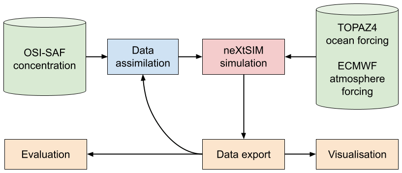
Figure 1Overall scheme of the neXtSIM-F forecasting platform. Blue block: data assimilation step (pre-processing); red block: running of the model core; light-brown blocks: post-processing steps; green blocks: input data. Note that we only assimilate OSI SAF SSMIS and AMSR2 concentrations.
3.1 The neXtSIM model
neXtSIM is a stand-alone sea-ice model which can use winds and currents from a variety of atmospheric and oceanic models (hindcasts or forecasts). This makes it quite flexible and light to run and therefore ideal for a forecasting context. Its dynamical core is the new brittle Bingham–Maxwell (BBM) rheology (Ólason et al., 2021). (The version of the BBM rheology corresponding to the results in this paper is also summarised in Appendix A.) Rampal et al. (2016) presented results using a previous version of neXtSIM including an elasto-brittle (EB) rheology as described in Bouillon and Rampal (2015), showing good agreement with observed drift and concentration in particular. More recently, Rampal et al. (2019) showed the ability to reproduce the characteristic multi-fractal scalings of deformation when using the previous version of neXtSIM, which included the Maxwell elasto-brittle (MEB) rheology (Dansereau et al., 2016). The key contribution of the MEB rheology was the addition of a viscous dissipation of stress in areas where the ice is damaged, allowing it to move more freely. However, in longer-term simulations the MEB showed unrealistic pile-up of ice particularly along the northeast coast of Greenland and the northwest coast of Svalbard. This led to the further addition of a frictional element to the rheology (Ólason et al., 2021), which provides some resistance to compression (up to a threshold). This framework, of a spring in series with a composite element made up a dashpot and fraction element in parallel, is called BBM.
The dynamical equations are solved with a finite element method on a Lagrangian (moving) triangular mesh. The code is currently a parallelised C++ code, used by Rampal et al. (2019), and presented by Samaké et al. (2017). Momentum input comes from the wind and ocean stresses (a turning angle of 25∘ is applied to the ocean velocity from the ocean forcing), the Coriolis force, and sea surface slope, and there is also a basal stress applied at the bottom of the ice when it becomes grounded. For this basal stress we follow the scheme of Lemieux et al. (2016b), using the parameters k1=10, k2=15 Pa m−1, αb=20, and m s−1.
There is also a thermodynamic component of the code, and beneath the ice is a slab ocean with three variables: temperature, salinity and thickness. The temperature and salinity are modified by the heat and salinity fluxes determined by the thermodynamical model as ice melts and freezes and as the model interacts with the atmosphere. They are relaxed towards the SST and SSS from TOPAZ over a timescale of about 1 month, while the thickness of the slab ocean is taken directly to be the MLD of TOPAZ. This varies spatially and evolves with time according to the forecast from TOPAZ. The thermodynamical model is a three-category model (detailed in Rampal et al., 2019, Appendix A): open water, newly formed ice (treated as one ice layer and one snow layer; Semtner, 1976) and older ice (treated as two ice layers and a snow layer; Winton, 2000).
The older ice is characterised in the model by concentration, c, and thickness averaged over the entire cell (effective thickness or, in other words, volume per unit area), h. The absolute thickness of ice can be computed as the ratio: ; there is also an effective snow thickness, s. The young ice has concentration cy, effective thickness hy, and snow thickness sy. The absolute thickness of young ice is constrained so that . If Hy<Hmin, cy is reduced to ; if Hy>Hmax, some ice is moved to the older ice category. During this process Hy is reduced to , while cy is also reduced to . This concentration reduction is intended to give some lateral decrease in young ice volume and not just vertical. The corrected values for hy and sy are and ); the corresponding properties for the older ice h, c and s are then increased in a ice-and-snow-volume-conserving manner. The values that we used for the thresholds on the absolute thin ice thickness are Hmin=0.05 m and Hmax=0.275 m.
The domain we present simulations for is a pan-Arctic one, with a resolution of about 7.5 km. A 7 d forecast for this domain runs in about 30 min using 16 processors.
3.2 Initialisation of the model fields
Before the model can be run it has to be initialised. (Note this is only done once and is not to be confused with the daily assimilation, which modifies the initial conditions for each new forecast). First, the triangular mesh for the destination domain is generated with Unref (a component of the open-source mesh-generation library GMSH: Geuzaine and Remacle, 2009) and using the Global Self-consistent, Hierarchical, High-resolution Shoreline Database (GSHHS) (Wessel and Smith, 1996). Then model variables like the ice concentration, the ice and snow thicknesses, and the temperature and salinity of the slab ocean are initialised. We use the CS2SMOS product (Sect. 2.5) to set the ice concentration and thickness, and we use the simulated sea surface temperature and salinity from TOPAZ4 (Sect. 2.1). The ice concentration in the CS2SMOS product comes from the low-resolution OSI SAF product (SSMIS), which is known to be too low in areas with low thickness (Ivanova et al., 2015). Therefore total sea ice concentration (ctot) is calculated by increasing the observed SIC according to the empirical formula:
where ccs2smos and hcs2smos are respectively the concentration and effective thickness in the CS2SMOS product, and a0=0.9569, a1=0.06787 and a2=0.4255 are parameters fitted from the observations (Thomas Lavergne, personal communication, 2019).
As mentioned above the model has two ice categories – young ice and older ice with different rheological behaviour. At the initialisation step young ice cy is set to comprise 20 % and the older ice c 80 % of the total SIC. If the observed absolute thickness is below the young ice upper thickness limit Hmax, then thickness is distributed between young and older ice in the same proportion; otherwise young ice thickness is calculated as and for the older ice: . It was identified that the model has little sensitivity to the fraction of young ice, and it may vary within 5 %–30 %.
The temperature and salinity of the slab ocean is taken to be equal to the TOPAZ4 surface forecast, while the ice velocity and damage are set to zero.
3.3 Assimilation of concentration
The assimilation is performed before each forecast run using the data insertion method – an updated (analysis) concentration () is calculated as a function of the forecast variable () and observations (cosisaf), the blended SSMIS/AMSR2 concentration from Eq. (1). Other variables (particularly ice and snow thicknesses and the SST of the slab ocean) are adjusted for consistency, the simulation is then restarted using the updated variables, and the model is run for 8 d to provide 1 d of hindcast and a 7 d forecast. The assimilation is performed on the model mesh – the satellite observations, originally provided on a regular grid, are linearly interpolated onto the centres of the mesh elements so that they can be directly compared with the neXtSIM prognostic variables.
The concentration update is done as follows. A target concentration is calculated using a weighted average approach:
The uncertainties of the observed concentration (σosisaf) are obtained from the input products (the root mean square of the SSMIS and AMSR2 errors), while the value for the uncertainty in the forecast concentration is set to 0.3 and can also be thought of as introducing a timescale (in days) of for relaxation towards the observations that depends on the relative uncertainties. Assimilation of concentration is performed in all elements that have valid observations.
In the pack, the total (young and old ice) model concentration ctot is generally close to 100 % (except inside leads and cracks), while the OSI SAF concentration can be around 90 %–95 %. We found that using ctarget as the actual update produced too much of a drop in the pack concentration, lowering the internal stress to near zero and allowing too much drift. This quickly led to rapid build-up of very thick ice in unusual places. Therefore we had to take a quite conservative approach to our correction and only change the model to make sure the ice mask (the part of the domain where the concentration is higher than 15 %) was correct (this is a kind of assimilation of extent):
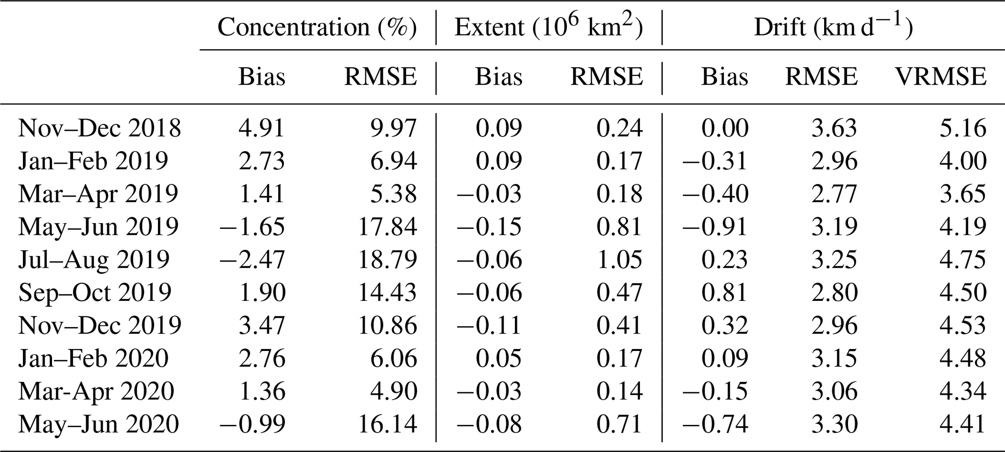
Table 1Accuracy of the free run. Concentration and extent are evaluated against OSI SAF SSMIS; thickness is evaluated against CS2-SMOS; drift is evaluated against OSI SAF drift, where observations with reported error up to 10 km d−1 are considered. Results are 2-monthly-averaged.
After calculating the updated variables as specified in Eq. (4) the fractions and thicknesses of young and older ice are calculated in the same way as in the initialisation procedure (see Sect. 3.2).
Once all the assimilation steps have been performed the model fields are checked for consistency with each other and corrected if necessary. First, the concentration of young ice is reduced in the elements where the total concentration exceeds 100 %. Second, the volume of ridged ice, damage, and the ice and snow thicknesses are set to zero in the added ice. Lastly, we need to correct the SST of the slab ocean. Where new ice is added during assimilation it is set to the freezing point, but if ice is removed then the situation is more complicated. Then we proceed as in the following section.
3.4 Compensating heat flux
One of the side effects of assimilation is that the heat balance in the model is disturbed: reducing the concentration opens more water, and depending on the temperatures, atmospheric humidity and ocean salinity provided by the forcing, the heat flux out of the ocean can increase dramatically, causing the ice to freeze up again very fast. This effect is strongest when the atmosphere is very cold. Therefore a compensating heat flux is added to the total ocean heat flux in order to keep the heat balance and prevent refreezing of ice where it was removed by assimilation, thus prolonging the effect of assimilation. If and are respectively the total concentrations before and after assimilation, a compensating heat flux (Qcomp) is calculated if ice was removed – i.e. if – according to the following formula:
where Qocean is the total heat flux from the ocean (sum of flux from the ocean to sea ice and to the atmosphere), and n is a parameter controlling the strength of correction. The function was chosen so that Qcomp is zero when the concentration update is zero, and when ; i.e. all the ice was removed by assimilation. With n=1 the reduction of Qcomp from 0 to −Qocean is linear, and with n>1 it becomes steeper for values of closer to . We use n=4 for the runs presented here, as this gives a suitably strong heat flux for a modest reduction in concentration.
We begin with an evaluation of a free run over the 20-month period from 1 November 2018 to 30 June 2020. This shows the general strengths and weaknesses of the model. We then evaluate the performance of the forecast system over this period to show the improvements gained by the assimilation of OSI SAF concentration.
4.1 Evaluation of free model run
In this section we demonstrate that the model is generally able to reproduce the overall drift, concentration and thickness patterns in observations. For all comparisons we average the model fields in time over an appropriate time window (in practice 1, 2 or 7 d), apply some spatial smoothing (being guided by the size of the satellite footprint) and interpolate onto the observation grid. For scalar variables, we define bias as 〈Vmod−Vobs〉 (with 〈⋅〉 defining the spatial mean over pixels where both model and observation are defined, and where either model or observations have ice). We also define RMSE as . For the ice extent, we define bias in extent as A10−A01, where A10 is the total area of pixels where neXtSIM predicts the presence of ice (total concentration greater than 15 %) but the observation has no ice, while A01 is the total area of pixels where neXtSIM predicts no ice but the observation does have ice. Instead of an RMSE, for the ice extent we define IIEE (integrated ice edge error, Goessling et al., 2016) as A10+A01. Thus the IIEE is always positive, and the bias is positive if neXtSIM is overestimating the total extent and negative if it is underestimating it. For the ice velocity we define the bias and RMSE as the mean and rms values of the difference in speed respectively – i.e. and . We also define the vector RMSE (VRMSE) as the rms of the vector difference, . Note that these drift errors can only be calculated where both model and observation have ice.
Table 1 shows 2-monthly summary statistics for observations that are available year-round (although they are much less reliable between May and September). Errors which are particularly high are the RMSE in ice concentration and the IIEE for extent between May and August – we will discuss reasons behind this below. The bias in these quantities is quite low, being highest between November and December, reflecting an ice advance which is too fast. The drift on the other hand compares quite well throughout the period, with the VRMSE being generally less than 4.5 km d−1 and the RMSE in speed less than 3.3 km d−1 (with the exception of the first 2 months). The bias is quite low, staying between ±0.8 km d−1. The first 2 months have a bias of zero, despite their high VRMSE and RMSE, with a Beaufort Gyre that is too slow cancelling a drift that is too fast in the triangle between the north pole, Svalbard and Franz Josef Land.
Table 2Accuracy of the free run for the 2018–2019 and 2019–2020 winters. Thickness is evaluated against CS2-SMOS and drift against OSI SAF drift, where only observations with reported error less than 1.25 km d−1 are considered. Results are 2-monthly-averaged.
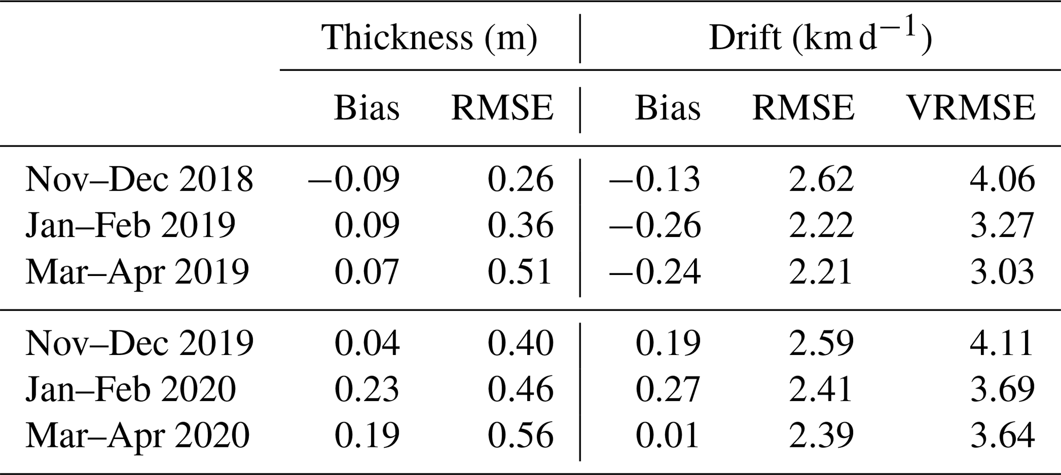
Table 2 shows the effect of restricting the drift evaluation to regions where the observational error is less than 1.25 km d−1. As discussed in Sect. 2.4 this removes the entire period from May to September, as well as the MIZ, the area around the north pole and areas close to the coast. Without the less accurate observations, the drop in VRMSE is between 0.3 and 1 km d−1, with their values now between 3 and 4.1 km d−1. However, the less accurate regions are also regions where the model has difficulties with other variables like thickness and extent, so this could also contribute to the reduction in error. Notwithstanding this, the November–December 2018 period is now much less of an outlier, now being quite close to November–December 2019. The RMSE in speed is now less than 2.6 km d−1, while the bias is between ±0.3 km d−1. There is a clear deterioration going from the first to the second winter.
Table 2 also summarises the comparison of model thickness with the CS2-SMOS product. RMSE is lower (0.26 m) in November–December 2018 since thickness was initialised using CS2-SMOS and grows to 0.51 m over the first winter. The RMSE grows from 0.4 to 0.56 m over the second winter. The bias is quite low in the first winter but about 0.2 m from January–April 2020.
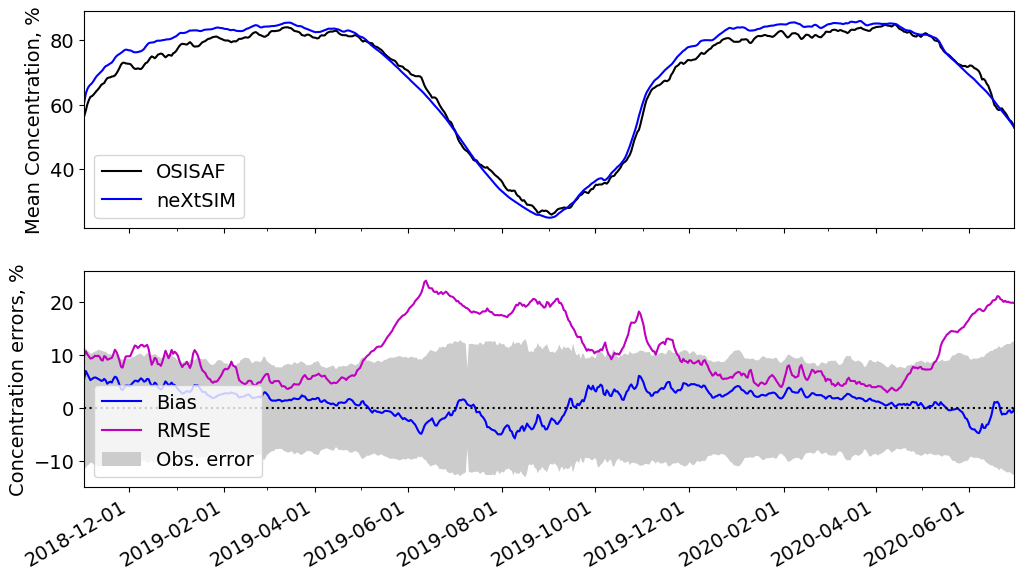
Figure 2Temporal comparison of model and OSI SAF SSMIS concentrations. The shaded area in the lower plot shows the rms uncertainty of the concentration for reference when considering the errors. The mean concentration is the mean over the ocean points in the domain, while the bias is defined as the mean error (model minus observation) over the region where either the model or observations have ice.
Figures 2 and 3 compare the mean concentration and extent from neXtSIM and the OSI SAF concentration product (see Sect. 2.3). Since we do not have enough information to create an error model for the concentration observations (for example it cannot be Gaussian due to its restriction to being between 0 % and 100 %) we could not generate confidence intervals for the mean concentration but instead plot a shaded area corresponding to for reference when considering the bias and RMSE in concentration. The seasonal cycle for mean concentration and extent is captured reasonably well, but the bias is clearly positive in winter and clearly negative in summer. As noted from Table 1 the RMSE in concentration and the IIEE are very high between mid-April and August. The RMSE in concentration is generally comparable to the rms error level outside these periods.
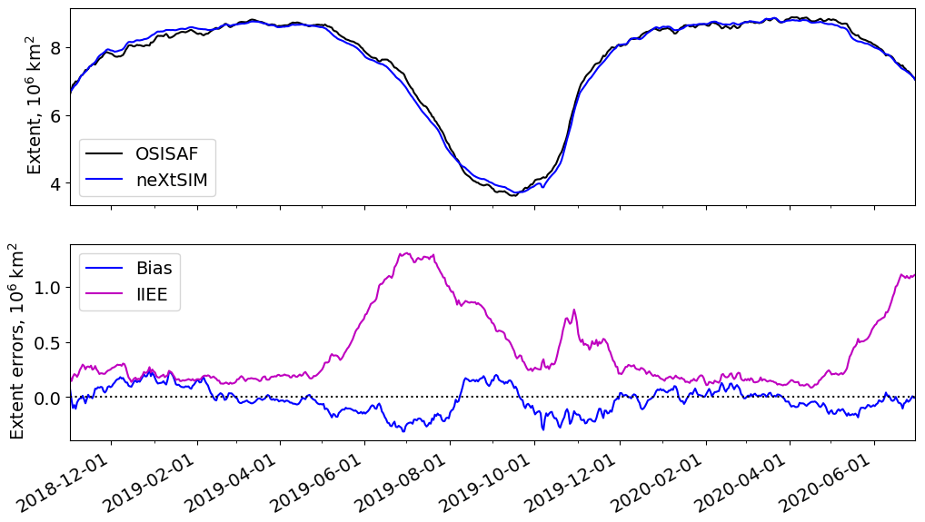
Figure 3Temporal comparison of extents (region where the concentration exceeds 15 %) from model and OSI SAF SSMIS concentrations. The bias is defined as modelled extent–observed extent.
In January–February there is a general overestimation in the pack as the model is approximately 100 % with some leads, while the SSMIS field has large regions of lower concentration that contribute to the errors (85 %–90 %). There is also a general overestimation in ice extent, which is also the case in November–December, primarily located in the Greenland Sea and the Barents seas. The areas north of Novaya Zemlya (around the Santa Anna Trough), around Franz Josef Land, and northwest of Svalbard stood out as places where the ice edge was not being located correctly. This continues into March–April and can be seen in Fig. 4, which shows selected maps of the concentration bias from March–October 2019. The region of underestimation to the northwest of Svalbard is related to the development of an arch between there and the northeast tip of Greenland. (This is also related to relatively large thicknesses in these areas, which increases the capacity of undamaged ice to stay undamaged.) This arching also reduces the ice export through the Fram Strait, the effect of which is seen in the maps for May–June and July–August. In May–June we also see that the ice that is in the Greenland Sea and is displaced too far to the east, producing a double penalty effect in the RMSE score. This is also a result of the arching in this area – the ice at the corner of Greenland is too thick to be exported, and so the ice that is exported has detached from the arch away from the coast and has then travelled roughly parallel to the coast without being pushed back towards it. In July–August the thicker ice has mostly melted and there is less of a dipole situation and more of a clear-cut underestimation.
Another problem area is around the Novosibirsk Islands (also known as New Siberian Islands) and the Laptev Sea. April sees the model opening slightly too far to the north; in May and June there is a strong underestimation to the north of the islands and too much fast ice. The underestimation is partly from melting that is too fast and from the fact that the fast ice has not detached and flowed into this area.
There is a similar problem to the west of Wrangel Island in the Chukchi Sea – an opening that is too large compared to the observations and with too much land-fast ice close to the coast which should be flowing into this region. There is also a large region of overestimation to the east of Wrangel Island, which is actually an artefact of the boundary conditions that we are using at the open Bering Strait boundary. If there is inflow at any open boundaries the value of any tracers is taken to be its value in the nearest mesh element, and in this case we have too much ice being imported through the Bering Strait, which leads to a build-up at this location.
The last things to mention about the July–August map are the strong overestimation around Franz Josef Land and the dipole situation in the Beaufort sea, which is the result of a Beaufort Gyre that is too slow.
However, by September–October, the situation has improved substantially. The main disagreement is in the ice edge from Severnaya Zemlya round to the just past Svalbard. This is due to an ice advance that is slightly too fast.
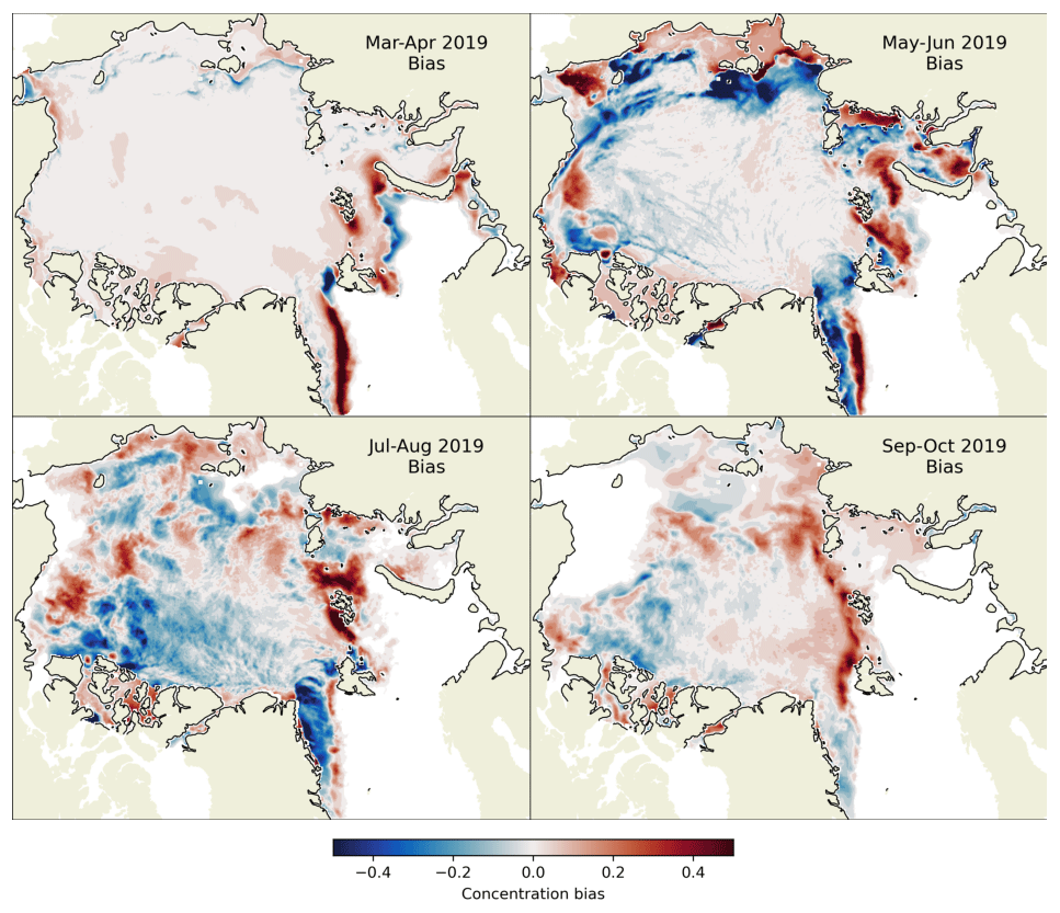
Figure 4Selected maps of the 2-monthly-averaged concentration biases between the free model run and from OSI SAF SSMIS. The bias is defined as model minus observation.
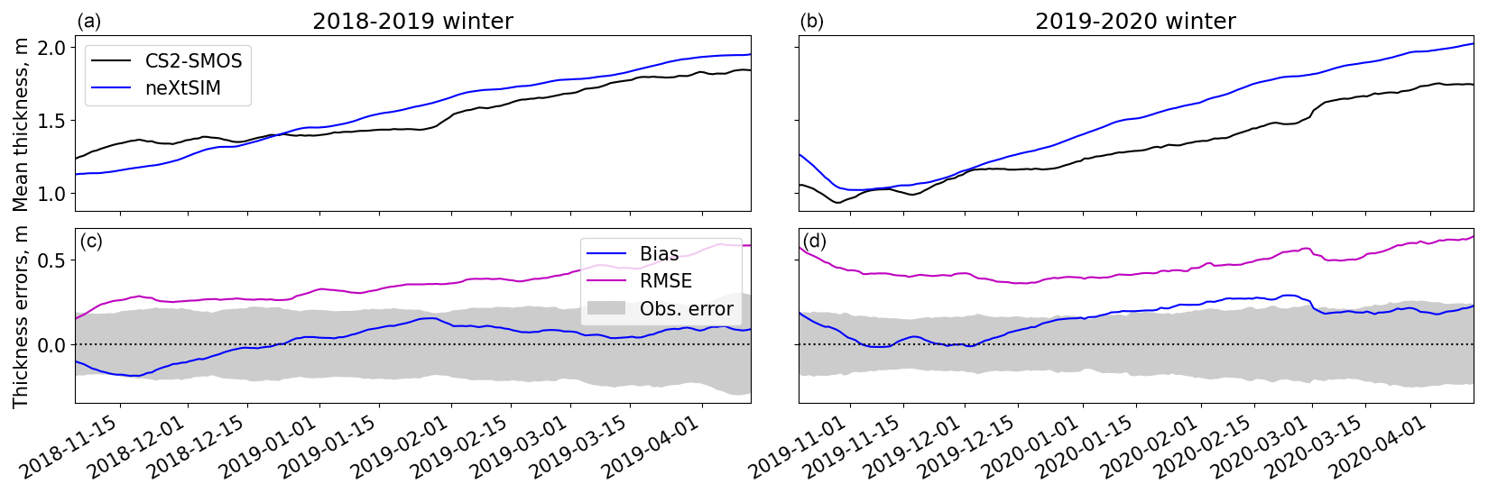
Figure 5Temporal comparison of model and CS2-SMOS thickness for two winters, 2018–2019 (a, c) and 2019–2020 (b, d). The shaded regions show the rms uncertainty in the CS2-SMOS product for reference. The mean thickness is the mean over the ocean points in the domain, while the bias is defined as the mean error (model minus observation) over the region where either the model or observations have ice.
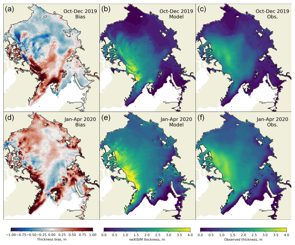
Figure 6Comparisons of time-averaged model and CS2-SMOS thickness for early (a–c) and late (d–f) in the 2019–2020 winter. (a, d) Bias maps; (b, e) neXtSIM thickness; (c, f) CS2-SMOS thickness. The bias is defined as model minus observation.
Figure 5 shows time series of mean thicknesses and of thickness errors when compared to CS2-SMOS, which have already been discussed to some extent in the context of Table 2. The mean observed and modelled thicknesses show a steady increase after November, but the modelled value is increasing faster than the observed one. The timing of when the modelled increase starts is close to when the observed increase starts. The lower plots have the rms uncertainties plotted for reference, and the model bias is generally at a similar level to this uncertainty. The RMSE is about twice this uncertainty in the second winter. We note here that the error levels in the CS2-SMOS product are only the interpolation error and are thus a lower bound as they do not include uncertainties in the individual CS2 and SMOS products. CS2 in particular is sensitive to the ice and snow densities used or the snow thickness which affect the conversion from freeboard to thickness (Zygmuntowska et al., 2014).
Figure 6 also shows the spatial distribution of the errors. Throughout the winter there is overestimation off the north coast of Greenland round to Axel Heiberg Island. Further to the west there is a thinning (but not an opening) from Axel Heiberg Island to Ellef Ringnes Island, which also seems to be related to the westward drift along this coast being too high. This persists throughout the winter, but the affected area reduces with time. In October–December there is a dipole pattern where the ice is too thin in the Beaufort Sea and too thick in the triangle between the north pole, Svalbard and Franz Josef Land. However, in January–April, this dipole reverses.
The modelled thickness is also quite high around the north of Svalbard, in contrast with the CS2-SMOS product, which has quite thin ice. This build-up contributes to the arching discussed in relation to the concentration errors, reducing the ice export through the Fram Strait. This stems from damaged ice not having enough resistance to compression. In the BBM rheology there is a balance between resisting compression enough to stop the build-up of ice at the coasts and resisting it so much that drift becomes too slow.
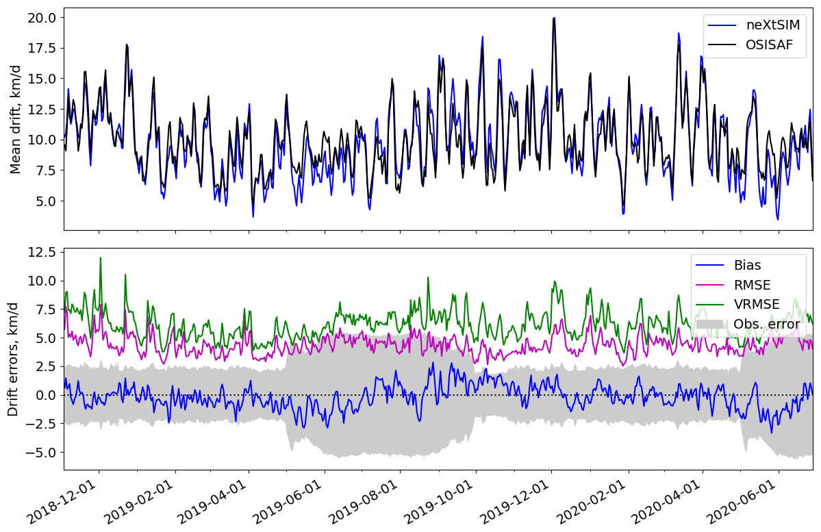
Figure 7Temporal comparison of model and OSI SAF drift. The shaded region shows the rms uncertainty in the OSI SAF drift product. The bias is defined as the mean modelled speed minus observed speed. The mean drift and errors are averages over the regions where both model and observations have valid drift vectors. Valid observations here are those that have reported errors less than 10 km d−1.
Figure 7 shows the drift bias and RMSE of neXtSIM when compared to the OSI SAF drift product. The shaded area corresponds to , where the factor of 2 comes from the fact that drift has two components. We also note that if one cell has components (xi,yi) with (not-necessarily Gaussian) noise (εi,δi) added to it (each with zero mean and variance ), the mean-squared drift in the presence of noise,
is higher than the noise-free (“true”) value 〈d2〉 by . It is tempting to then just subtract this amount from the speed when comparing with the model, but we decided that the uncertainty in the quoted uncertainty could be too influential and also that the model drift has some unknown uncertainty associated with it, so we persisted with directly comparing the drift in the OSI SAF product with the model drift in order to judge when the model is too fast or too slow and plotted the error level for reference. The difference in speed (model speed minus observed speed) fluctuates somewhat but stays largely within the error limits. The rms error for this product is approximately 1.8 km d−1 from October to May but increases to about 4 km d−1 from May to September. However, the model is starting to show signs of being too slow in April and May 2020. The RMSE in speed ranges between about 3–4.5 km d−1, which is outside the estimated error for the more accurate colder months. The VRMSE (vector RMSE) is higher than the RMSE by about 1.5 km d−1.
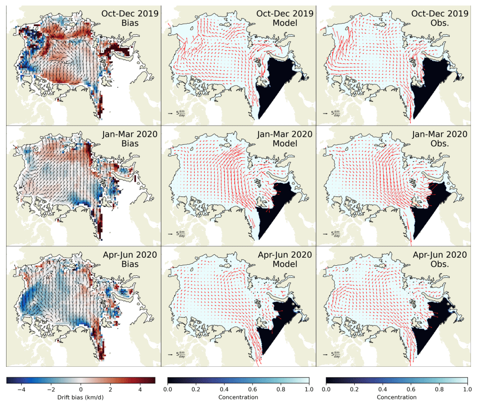
Figure 8Comparisons of 2-monthly-averaged model and OSI SAF drift from the 2019–2020 winter. The drift bias colour maps (left column) show the bias in speed, while the directions show the difference between the model and observation directions (arrows pointing up indicate the directions are the same). The central column shows ice velocity vectors from neXtSIM, while the right-hand column shows OSI SAF vectors. The concentration colour maps show the average neXtSIM concentration over the analysis period. The bias is defined as modelled speed minus observed speed.
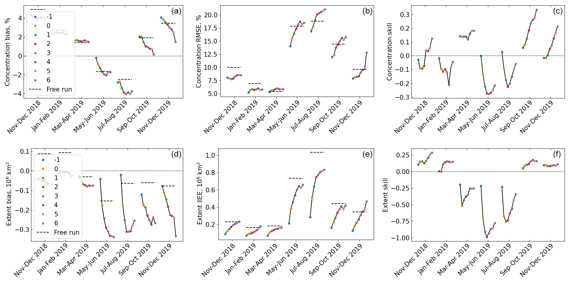
Figure 9Two-monthly-averaged forecast errors grouped by lead time (lead times are indicated in the figure legends). The free run errors for the corresponding periods are plotted as dotted lines for reference on the bias and RMSE/IIEE plots. (a–c) Two-monthly-averaged bias, RMSE and forecast skill for concentration grouped by lead time. (d–f) Two-monthly-averaged bias, IIEE and forecast skill for extent grouped by lead time.
Figure 8 shows the general spatial pattern in the drift errors. The maps for October–December 2019 show that the general circulation of the model and the observations are agreeing well, with the main feature being the gyre in the central Arctic Ocean. However, this gyre is slightly too fast and there is also too much westward drift along the Canadian Arctic Archipelago. The observations also show a small gyre in the East Siberian Sea which is not apparent in the model drift. The strongest positive bias is in the Kara Sea although the errors in the observations are high there, being close to the coast and the MIZ. The model is also showing strong positive biases in the Laptev and East Siberian seas where the ice is thinner. On the other hand, the drift in the Beaufort and Chukchi seas is too slow.
In January–March 2020, the general pattern in the observations is a strong flow from the Laptev over to the Greenland Sea, with a weaker transpolar drift from the Chukchi Sea joining this outflow. The model also produces the flow from the Laptev Sea, but the flow from the Chukchi Sea is more directed towards the Beaufort Sea than across to the Greenland Sea. This may be contributing to the biases seen in the thicknesses – too thick in the Beaufort Sea while too thin in the region between the Laptev and Greenland seas. The drift is also starting to become too slow north of Greenland and Svalbard, and this is most likely due to the ice build-up in those areas.
In April–June 2020 there is a stronger Beaufort Gyre and a similarly strong cyclonic gyre in the Laptev Sea. These connect to form quite a wide stream from the central Arctic to the Greenland Sea. While the model captures the gyre in the Laptev Sea, the Beaufort Gyre is less well defined in this period, possibly due to the ice being too thick in the Beaufort Sea at this time. As in January–March, drift is also too slow to the north of Greenland.
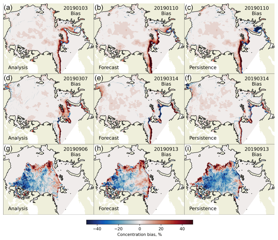
Figure 10Selected maps of daily-averaged biases in concentration compared to OSI SAF SSMIS for three examples of forecasts, starting on 3 January 2019 (a–c, positive skill) and the other on 7 March 2019 (d–f, negative skill) and 6 September 2019 (g–i, positive). Panels (a), (d) and (g) show the evaluation for the first day of simulation (lead time −1: analysis or hindcast), while panels (b), (e) and (h) show the evaluation for the eighth day of simulation (lead time 7). Panels (c), (f) and (i) show the bias in the persistence forecast (defined as the results for the first day of simulation) for lead time 7. The bias is defined as model minus observation.
4.2 Evaluation of forecasts with assimilation
The performance of the forecasting system with assimilation of concentration was evaluated over the same period as the free run was in Sect. 4.1 (that is the 20 months from November 2018 to the end of June 2020). In order to reduce computation time, the 7 d forecasts were launched approximately only every 7 d, with 1 d analyses being launched in between so that the assimilation was still performed daily.
The model performance was evaluated against satellite observations of the sea ice SSMIS concentration and drift from OSI SAF (see Sect. 2.3 and 2.4). The metrics we used in our assessment were bias and RMSE in concentration; bias and IIEE in extent; and bias, RMSE and VRMSE in drift. A persistence forecast of concentration (the initial concentration, defined for technical convenience as the average of the first hour) was used as a benchmark for concentration and extent, and forecast skill was defined as
Thus, a model that is agreeing perfectly with the observations has skill equal to 1, while it is negative (with no lower bound) if the persistence error is lower than the forecast error. We decided that given the strong dependence of drift on wind, its rapid variability in time would render a persistence forecast for drift quite easy to beat, so for this variable we just present the forecast errors. However, we can make some rough comparisons to the drift errors of other products, even though they use different observations for their evaluation so we cannot make a direct comparison. We note that the drift from the TOPAZ forecast generally has a bias in speed of about 2 km d−1 and a VRMSE of about 5–8 km d−1 Melsom et al. (2018), while Metzger et al. (2017) report an rms drift speed error of about 5–8 km d−1 in the Arctic for the GOFS 3.1 system.
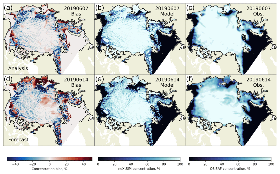
Figure 11Maps of daily-averaged biases (a, d) in concentration compared to OSI SAF SSMIS, and modelled (b, e) and observed (c, f) concentrations, for an example forecast starting on 6 June 2019. Panels (a)–(c) show the comparison for the first day of simulation, while panels (d)–(f) show the comparison for the eighth day of simulation. The bias is defined as model minus observation.
Figure 9 shows the 2-monthly averages for the different metrics applied to the concentration and extent. We only plot results for the first year and 2 months, since the error statistics from the 2020 results were nearly identical to the previous years. As with the free run, the concentration from the forecast is generally higher than OSI SAF in the winter months. As mentioned earlier, we do not try to correct this as reducing the concentration in the pack causes serious problem with the drift and thickness. The extent, which is adjusted during assimilation, is also lower than the observed one for the whole period, by differing amounts. Figure 10 shows some example forecasts from winter and autumn – one from January, March and September 2019 respectively. The first and third examples are forecasts with positive skill in extent (model does better than persistence), while the second has negative skill. However, they all have relatively low IIEE and RMSE in concentration. The January example shows that the rapid advance in the Kara Sea is captured relatively well by the model, and while the extent in the Greenland and Barents seas is too high, the ice edge is quite variable, and the model is doing better than the persistence at this time. The March example shows an example where there is quite a persistent negative bias to the northwest of Svalbard and in the Barents Sea. These errors probably originate in the ocean forcing, which we are unable to overcome even with our flux compensation. The persistence forecast does well in this example since the ice conditions are not changing very much. In the September example, the bias is similar to the free run, but it has been reduced by the assimilation. There is still an ice advance that is too fast in the European Arctic, but it is closer to the observations than the persistence forecast.
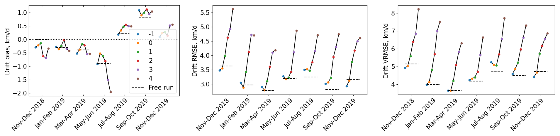
Figure 12Two-monthly-averaged bias, RMSE and VRMSE for drift grouped by lead time (lead times are indicated in the figure legends). The lead times refer to the start of each 2 d drift evaluation period – e.g. “0” covers the period from day 0 (12:00) to day 2 (12:00). The free run errors for the corresponding periods are plotted as dotted lines for reference. The bias is defined as modelled speed minus observed speed.
In the summer, the forecasts are systematically lower in concentration, partly due to differences in the pack, which we do not correct for, and in the extent. We are not too concerned by differences in the pack, as the differences are still comparable to observation error. Differences in the extent however are more concerning. In the summer, the forecasts score particularly badly with this metric, largely due to the dynamical problems also seen in the free run: arching above the Fram Strait, as well as fast ice in the Laptev and East Siberian seas that is too slow to detach. Figure 11 shows a typical example from this time period. Despite the correction in extent during assimilation, the ice that is added in the Fram Strait is quite thin and it melts quite quickly.
Figure 12 shows the bias, RMSE and VRMSE for the forecast drift. For smaller lead times it has similar quality to the free run, which is to be expected since the assimilation does not modify fields in the pack, with minor differences that are probably just due to differences in extent determining which observations are included or not. There is a small negative bias in speed in the winter months and a slight positive bias in the summer. The bias is not showing a large variability with forecast lead time, although there are some exceptions. With the exception of the first 2 months, which is slightly higher than the others, the RMSE (RMSE in speed) is quite consistent throughout the whole evaluation period, with a steady increase with lead time. The RMSE for the final day is still mostly less than 5 km d−1. The VRMSE, which evaluates the drift direction as well as its speed, shows a larger dependence on lead time, starting between 4.5–5 km d−1 but getting up to between 7–8 km d−1 by the final day (occasionally being under 7 km d−1 or over 8 km d−1). This dependence on lead time is almost certainly due to increasing inaccuracy in the forecast winds.
neXtSIM-F became operational in July 2020 as part of CMEMS, and this paper presents an upgraded version that will be included in December 2020. Here we have evaluated the neXtSIM model itself in a free run for the period 1 November 2018 to 30 June 2020, as well as the neXtSIM-F forecast platform which corrects the initial conditions daily by assimilating sea ice concentration.
The free run, which used hindcast winds, had good drift, being relatively unbiased and having a low RMSE in speed of 3–4 km d−1. The RMSE was closer to 2.5 km d−1 when less accurate observations (uncertainty less than 2.5 km for the 2 d drift) were filtered out, although the observations so removed would also be near the coast and in the MIZ where we do have problems with thickness and extent respectively. Considering the VRMSE, the RMSE in the final position of each trajectory added about 1 km d−1.
The model thickness was biased slightly too thick in general, and there was also a tendency to have a dipole behaviour with one or too areas being too thick and one or two being too thin. The location of these regions that are too thin varied over the winter (the only time when the CS2-SMOS observations were available), but the thickness off northeast Greenland and north Svalbard was invariably too high. This caused the formation of an arch across the Fram Strait, which limited the export of ice through this strait in the summer, especially close to the coast.
When we evaluated the concentration and extent we found that the sea ice extent in the summer was greatly affected by the arching mentioned above, in that the total extent was too small and that the ice was also displaced from where it should be – there was no ice close to the east coast of Greenland (unlike in the observations), and it extended too far to the east.
There were also less severe differences in the ice edge which were probably partly due to errors in the ocean and/or atmospheric forcings, but the other big issue was the extent of the land-fast ice in May and June in the Laptev and East Siberian seas – this was too slow to detach and also contributed to there being too little ice further away from the coast at this time.
Owing to the fairly conservative approach that we had to take to the assimilation, the forecasts generally had the same properties as the free run with regards to thickness and drift. The bias in drift remains close to zero for the whole 8 d simulation, although the RMSE in speed and the VRMSE begin to deteriorate after about 4–5 d of simulation (up to a lead time of 4) – this is almost certainly due to less accurate winds at these lead times. The forecasts also had greatly improved IIEE scores compared to the free run. However, the more serious problems with the summer extent – in the Greenland Sea (due to arching) and to a lesser degree the Laptev and East Siberian seas (land fast ice) – were still present in the forecasts. The land-fast ice could possibly be improved with further tuning of the basal grounding scheme, while the arching problem is more difficult to solve. However, recent experiments indicate that changing the role of concentration in the rheology could give some improvements here – note that the viscous relaxation time in Eq. (A3) and thus the entire left-hand side of Eq. (A2) only depend on damage and not on concentration, so larger stresses do not drop very quickly if the ice is undamaged and the concentration drops (low concentrations cause the right-hand side of Eq. A2 to drop to near zero). There may be additional modifications to the rheology that could be made to help reduce arching in this region.
Assimilation of different data might also help.
-
Sea ice thickness. We could use either the hybrid CS2-SMOS product or the CS2 trajectories themselves to limit the build-up of ice on either side of the Fram Strait. However, these data stop in mid-April, so build-up that occurs later may still be enough to cause the arching.
-
Sea ice deformation Korosov and Rampal (2017) were able to derive sea ice drift from SAR data using a combination of feature tracking and pattern matching. Deformation can then be calculated to modify the damage variable and thus induce break-up at the right place. Unfortunately, this option is also time-limited as surface melt makes the ice smoother and stops the feature tracking algorithm from working as effectively.
Another possibility could be to take the approach of Ying (2019) and to morph the modelled ice mask onto the observed one so that, for example, ice in the Greenland sea could be moved over towards the coast, instead of removing thicker ice at the ice edge and adding thinner ice towards the coast. Possibly a better source of ice extent than OSI SAF concentration could also be used in conjunction with such a morphing approach. For example, the United States Naval Ice Center6 produces daily, pan-Arctic ice charts. Other alternatives for assimilating extent are MASIE (Multisensor Analyzed Sea Ice Extent: Fetterer et al., 2010) and IMS (Interactive Multisensor Snow and Ice Mapping System: Helfrich et al., 2007), as done by the GOFS 3.1 system for example. Automatic ice type classification from SAR is also possible now – for example the algorithm developed by Park et al. (2020) and upgraded by Boulze et al. (2020) will become operationally distributed by CMEMS in 2021.
A framework to produce an ensemble forecast with neXtSIM-F is also being developed (Cheng et al., 2021, as a follow-up of the work of Rabatel et al., 2018), with the ultimate aim of using the ensemble Kalman filter (EnKF) assimilation method. Work on using EnKF with models running on adaptive meshes (like neXtSIM) is being developed in parallel at the Nansen Environmental and Remote Sensing Center (NERSC; Aydoğdu et al., 2019). This may also be effective at addressing some of the errors in the forecast.
Finally, in order to provide more consistent ocean inputs to the sea ice model (as well as to provide more realistic stresses and fluxes to the ocean model), work is ongoing to couple neXtSIM with the ocean models HYCOM and NEMO and to add an atmospheric boundary layer model to mediate between the atmospheric model and the ice and/or ocean models. Also, neXtSIM is already coupled to the WAVEWATCH 3 wave model (Boutin et al., 2021), so there is scope for neXtSIM-F to include more components like wave and ocean models.
We refer readers to Rampal et al. (2019) for most of the details but give some important modifications below. The momentum balance is
where is the ice velocity, ρi is the density of ice, hy is the mean young ice thickness, h is the mean thickness of older ice, σ is the internal stress, σP is an additional plastic stress that is most active when damaged ice is under convergence, τ is the sum of stresses applied by the wind and ocean currents and by keels grounding on the sea floor, f is the Coriolis parameter, , g is the acceleration due to gravity, and η is the sea surface height.
There is an evolution equation for the damage (d), which is unchanged from Rampal et al. (2019, see Eqs. A8–A15). The rheology consists of a friction element and a dashpot in parallel, as well as a spring in series with this parallel element. Accordingly the stress follows the constitutive relation
where K is the stiffness tensor (see Eq. A4 of Rampal et al., 2019), is the deformation rate tensor, E is Young's modulus and λ is the viscous relaxation time. E and λ vary according to the damage and the concentration of old ice c
Here E0 is Young's modulus for undamaged ice at 100 % concentration, λ0 is the (large) value of λ for undamaged ice and α>1 is an exponent which can be tuned to control how fast λ drops due to damaging. Note we do not consider young ice in the constitutive relations since it is assumed to be weak. The term depends on the normal stress (defined to be positive under convergent conditions) and particularly on whether the ice is converging or not:
where the different regimes are (i) diverging, (ii) converging and elastic, and (iii) converging and ridging. Also, is the concentration- and thickness-dependent threshold for when the Bingham element starts moving (P* is a constant tuning parameter of the order of 10 kPa). If σn<0, the friction element is inactive and the dashpot is free to move, and the internal stress is quickly dissipated in damaged areas. If , the friction element is active and stationary, which also stops the dashpot from moving and dissipating stress. Thus even highly damaged ice is able to resist compression. However, once σn>Pmax, the friction element starts to move, the dashpot becomes active again and the ice starts to ridge.
The MEB rheology as presented by Rampal et al. (2019) corresponds to the situation where is always 1 in Eq. (A4). In addition, the term involving in Eq. (A2) was not present (it was required to stabilise the explicit solution of the BBM equations). In the first version of our CMEMS forecast (which ran from July–December 2020), two modifications were made to the version of MEB in Rampal et al. (2019):
- i.
In Eq. (A3a) for E, d was taken to be zero if it was less than 0.95, which helped to improve localisation of deformation.
- ii.
An extra stress σP was added to σ in the momentum equation (Eq. A1), which provided some resistance to compression. This stress was given by
where was a tuning parameter of the order of 10 kPa, and δP was a small parameter needed for numerical stability.
Real-time forecast data and best estimates can be accessed through the Copernicus Marine Environment Monitoring Services portal (https://resources.marine.copernicus.eu/?option=com_csw&view=details&product_id=ARCTIC_ANALYSISFORECAST_PHY_ICE_002_011, last access: 8 July 2021, Copernicus Marine Environment Monitoring Services, 2021).
TW and AK wrote the paper and did the experiments. PR and EO contributed to writing and planning the paper and experiments. EO was also behind many background developments in the model code.
The authors declare that they have no conflict of interest.
Publisher’s note: Copernicus Publications remains neutral with regard to jurisdictional claims in published maps and institutional affiliations.
We would like to acknowledge Véronique Dansereau for interesting discussions on the MEB and BBM rheology; Abdoulaye Samaké, who parallelised the neXtSIM code; and Mika Malila, who contributed to our evaluation scripts. Finally, we would like to thank Sylvain Bouillon and Philip Griewank for their original contribution to building a forecasting system around the neXtSIM sea ice model. Computing and storage resources were provided by UNINETT Sigma2 – the National Infrastructure for High Performance Computing and Data Storage in Norway (projects NN2993K and NS2993K).
This research has been supported by the Norwegian Research Council (neXtWIM (grant no. 244001) and Nansen Legacy (grant no. 276730)), the European Commission (SWARP (grant no. 607476)), the Service hydrographique et océanographique de la Marine (IMPSIM (grant no. 30 18CP10)), Copernicus Marine Environment Monitoring Services (contract no. 69), and the European Space Agency through the Cryosphere Virtual Laboratory (CVL, grant no. 4000128808/19/I-NS).
This paper was edited by John Yackel and reviewed by Jean-François Lemieux and one anonymous referee.
Aydoğdu, A., Carrassi, A., Guider, C. T., Jones, C. K. R. T., and Rampal, P.: Data assimilation using adaptive, non-conservative, moving mesh models, Nonlin. Processes Geophys., 26, 175–193, https://doi.org/10.5194/npg-26-175-2019, 2019. a
Azzara, A. J., Wang, H., Rutherford, D., Hurley, B. J., and Stephenson, S. R.: A 10-year projection of maritime activity in the US Arctic region, Tech. rep., The International Council on Clean Transportation, Washington, DC, 2015. a
Bleck, R.: An oceanic general circulation model framed in hybrid isopycnic-Cartesian coordinates, Ocean Model., 4, 55–88, 2002. a
Bouillon, S. and Rampal, P.: Presentation of the dynamical core of neXtSIM, a new sea ice model, Ocean Model., 91, 23–37, https://doi.org/10.1016/j.ocemod.2015.04.005, 2015. a
Boulze, H., Korosov, A., and Brajard, J.: Classification of sea ice types in Sentinel-1 SAR data using convolutional neural networks, Remote Sensing, 12, 2165, https://doi.org/10.3390/rs12132165, 2020. a
Boutin, G., Williams, T., Rampal, P., Olason, E., and Lique, C.: Wave–sea-ice interactions in a brittle rheological framework, The Cryosphere, 15, 431–457, https://doi.org/10.5194/tc-15-431-2021, 2021. a
Cheng, S., Aydoğdu, A., Rampal, R., Carassi, A., and Bertino, L.: Probabilistic forecasts of sea ice trajectories in the Arctic: impact of uncertainties in surface wind and ice cohesion, Oceans, 1, 326–342, https://doi.org/10.3390/oceans1040022, 2021. a
Copernicus Marine Environment Monitoring Services: Arctic Ocean Sea Ice Analysis and Forecast, available at: https://resources.marine.copernicus.eu/?option=com_csw&view=details&product_id=ARCTIC_ANALYSISFORECAST_PHY_ICE_002_011, last access: 8 July 2021. a
Dansereau, V., Weiss, J., Saramito, P., and Lattes, P.: A Maxwell elasto-brittle rheology for sea ice modelling, The Cryosphere, 10, 1339–1359, https://doi.org/10.5194/tc-10-1339-2016, 2016. a, b
Drange, H. and Simonsen, K.: Formulation of air-sea fluxes in the ESOP2 version of MICOM, Tech. Rep. 125, Nansen Environmental and Remote Sensing Center, Bergen, Norway, 1996. a
Fetterer, F., Savoie, M., Helfrich, S., and Clemente-Colón, P.: Multisensor Analyzed Sea Ice Extent – Northern Hemisphere (MASIE-NH), Version 1, https://doi.org/10.7265/N5GT5K3K, 2010. a
Geuzaine, C. and Remacle, J.-F.: Gmsh: A 3-D finite element mesh generator with built-in pre- and post-processing facilities, Int. J. Numer. Method. Eng., 79, 1309–1331, https://doi.org/10.1002/nme.2579, 2009. a
Goessling, H. F., Tietsche, S., Day, J. J., Hawkins, E., and Jung, T.: Predictability of the Arctic sea ice edge, Geophys. Res. Lett., 43, 1642–1650, https://doi.org/10.1002/2015GL067232, 2016. a
Helfrich, S. R., McNamara, D., Ramsay, B. H., Baldwin, T., and Kasheta, T.: Enhancements to, and forthcoming developments in the Interactive Multisensor Snow and Ice Mapping System (IMS), Hydrol. Process., 21, 1576–1586, 2007. a
Hunke, E., Allard, R., Blain, P., Blockley, E., Feltham, D., Fichefet, T., Garric, G., Grumbine, R., Lemieux, J.-F., Rasmussen, T., Ribergaard, M., Roberts, A., Schweiger, A., Tietsche, S., Tremblay, B., Vancoppenolle, M., and Zhang, J.: Should Sea-Ice Modeling Tools Designed for Climate Research Be Used for Short-Term Forecasting?, Curr. Clim. Change Rep., 6, 121–136, 2020. a, b
Hunke, E. C. and Dukowicz, J. K.: An Elastic–Viscous–Plastic Model for Sea Ice Dynamics, J. Phys. Oceanogr., 27, 1849–1867, 1997. a
Hunke, E. C. and Lipscomb, W. H.: CICE: the Los Alamos Sea Ice Model Documentation and Software User’s Manual Version 4.1, Tech. Rep. LA-CC-06-012, T-3 Fluid Dynamics Group, Los Alamos National Laboratory, 2010. a
Ivanova, N., Pedersen, L. T., Tonboe, R. T., Kern, S., Heygster, G., Lavergne, T., Sørensen, A., Saldo, R., Dybkjær, G., Brucker, L., and Shokr, M.: Inter-comparison and evaluation of sea ice algorithms: towards further identification of challenges and optimal approach using passive microwave observations, The Cryosphere, 9, 1797–1817, https://doi.org/10.5194/tc-9-1797-2015, 2015. a
Kaleschke, L., Tian-Kunze, X., Maaß, N., Beitsch, A., Wernecke, A., Miernecki, M., Müller, G., Fock, B. H., Gierisch, A. M., Schlünzen, K. H., Pohlmann, T., Dobrynin, M., Hendricks, S., Asseng, J., Gerdes, R., Jochmann, P., Reimer, N., Holfort, J., Melsheimer, C., Heygster, G., Spreen, G., Gerland, S., King, J., Skou, N., Søbjærg, S. S., Haas, C., Richter, F., and Casal, T.: SMOS sea ice product: Operational application and validation in the Barents Sea marginal ice zone, Remote Sens. Environ., 180, 264– 273, https://doi.org/10.1016/j.rse.2016.03.009, 2016. a
Korosov, A. A. and Rampal, P.: A combination of feature tracking and pattern matching with optimal parametrization for sea ice drift retrieval from SAR data, Remote Sensing, 9, 258, https://doi.org/10.3390/rs9030258, 2017. a, b
Lavelle, J., Tonboe, R., Pfeiffer, H., and Howe, E.: Product User Manual for the OSI SAF AMSR-2 Global Sea Ice Concentration, Tech. Rep. SAF/OSI/CDOP2/DMI/TEC/265, Danish Meteorological Institute, available at: http://osisaf.met.no/docs/osisaf_cdop2_ss2_pum_amsr2-ice-conc_v1p1.pdf (last access: 2 July 2021), 2016a. a
Lavelle, J., Tonboe, R., Pfeiffer, H., and Howe, E.: Validation Report for The OSI SAF AMSR-2 Sea Ice Concentration, Tech. Rep. SAF/OSI/CDOP2/DMI/SCI/RP/259, Danish Meteorological Institute, available at: http://osisaf.met.no/docs/osisaf_cdop2_ss2_valrep_amsr2-ice-conc_v1p1.pdf (last access: 2 July 2021), 2016b. a
Lavelle, J., Tonboe, R., Jensen, M., and Howe, E.: Product user manual for osi saf global sea ice concentration, Tech. Rep. SAF/OSI/CDOP2/DMI/SCI/RP/225, Danish Meteorological Institute, 2017. a
Lavergne, T.: Validation and Monitoring of the OSI SAF Low Resolution Sea Ice Drift Product, Tech. Rep. SAF/OSI/CDOP/Met.no/T&V/RP/131, Norwegian Meteorological Institute, 2010. a
Lavergne, T. and Eastwood, S.: Low Resolution Sea Ice Drift Product User’s Manual, Tech. Rep. SAF/OSI/CDOP/met.no/TEC/MA/128, Norwegian Meteorological Institute, 2010. a, b
Lavergne, T., Eastwood, S., Teffah, Z., Schyberg, H., and Breivik, L.-A.: Sea ice motion from low-resolution satellite sensors: An alternative method and its validation in the Arctic, J. Geophys. Res.-Oceans, 115, C10032, https://doi.org/10.1029/2009JC005958, 2010. a
Lemieux, J.-F., Beaudoin, C., Dupont, F., Roy, F., Smith, G. C.,Shlyaeva, A., Buehner, M., Caya, A., Chen, J., Carrieres, T., Pogson, L., DeRepentigny, P., Plante, A., Pestieau, P., Pellerin, P., Ritchie, H., Garric, G., and Ferry, N.: The Regional Ice Prediction System (RIPS): verification of forecast sea ice concentration, Q. J. Roy. Meteor. Soc., 142, 632–643 2016a. a
Lemieux, J.-F., Dupont, F., Blain, P., Roy, F., Smith, G. C., and Flato, G. M.: Improving the simulation of landfast ice by combining tensile strength and a parameterization for grounded ridges, J. Geophys. Res.-Oceans, 121, 7354–7368, https://doi.org/10.1002/2016JC012006, 2016b. a
Marsan, D., Stern, H., Lindsay, R. W., and Weiss, J.: Scale dependence and localization of the deformation of Arctic sea ice, Phys. Rev. Lett., 93, 178501, https://doi.org/10.1103/PhysRevLett.93.178501, 2004. a
Meier, W. N.: Losing Arctic sea ice: Observations of the recent decline and the long-term context, 3 edn., chap. 11, in: Sea Ice, edited by: Thomas, D. N., John Wiley & Sons, 290–303, 2017. a
Melsom, A., Simonsen, M., Bertino, L., Hackett, B., Waagbø, G. A., and Raj, R.: Quality Information Document For Arctic Ocean Physical Analysis and Forecast Product ARCTIC_ANALYSIS_FORECAST_PHYS_002_001_A, Tech. Rep. CMEMS-ARC-QUID-002-001a, Norwegian Meteorological Institute, 2018. a
Metzger, E., Helber, R. W., Hogan, P. J., Posey, P. G., Thoppil, P. G., Townsend, T. L., Wallcraft, A. J., Smedstad, O. M., Franklin, D. S., Zamudo-Lopez, L., and Phelps, M. W.: Global Ocean Forecast System 3.1 validation test, Tech. rep., Naval Research Laboratory, Stennis Space Center, 2017. a
Ólason, E., Boutin, G., Korosov, A., Rampal, P., Williams, T., Kimmritz, M., Dansereau, V., and Samaké, A.: A new brittle rheology and numerical framework for large-scale sea-ice models, in preparation, 2021. a, b, c, d
Overland, J. E., Hanna, E., Hanssen-Bauer, I., Kim, S.-J., Walsh, J. E., Wang, M., Bhatt, U. S., and Thoman, R. L.: Surface air temperature, in: Arctic Report Card 2018, NOAA, available at: https://www.arctic.noaa.gov/Report-Card/Report-Card-2018 (last access: 6 July 2021), 2018. a
Owens, R. G. and Hewson, T.: ECMWF Forecast User Guide, Tech. rep., ECMWF, Reading, https://doi.org/10.21957/m1cs7h, 2018. a, b
Park, J.-W., Korosov, A. A., Babiker, M., Won, J.-S., Hansen, M. W., and Kim, H.-C.: Classification of sea ice types in Sentinel-1 synthetic aperture radar images, The Cryosphere, 14, 2629–2645, https://doi.org/10.5194/tc-14-2629-2020, 2020. a
Perovich, D., Meier, W., Tschudi, M., Farrell, S., Hendricks, S., Gerland, S., Haas, C., Krumpen, T., Polashenski, C., Ricker, R., and Webster, M.: Sea ice, in: Arctic Report Card 2018, NOAA, available at: https://www.arctic.noaa.gov/Report-Card/Report-Card-2018 (last access: 6 July 2021), 2018. a
Rabatel, M., Rampal, P., Carrassi, A., Bertino, L., and Jones, C. K. R. T.: Impact of rheology on probabilistic forecasts of sea ice trajectories: application for search and rescue operations in the Arctic, The Cryosphere, 12, 935–953, https://doi.org/10.5194/tc-12-935-2018, 2018. a
Rampal, P., Weiss, J., Marsan, D., Lindsay, R., and Stern, H.: Scaling properties of sea ice deformation from buoy dispersion analysis, J. Geophys. Res., 113, C03002, https://doi.org/10.1029/2007JC004143, 2008. a
Rampal, P., Bouillon, S., Ólason, E., and Morlighem, M.: neXtSIM: a new Lagrangian sea ice model, The Cryosphere, 10, 1055–1073, https://doi.org/10.5194/tc-10-1055-2016, 2016. a, b, c
Rampal, P., Dansereau, V., Olason, E., Bouillon, S., Williams, T., Korosov, A., and Samaké, A.: On the multi-fractal scaling properties of sea ice deformation, The Cryosphere, 13, 2457–2474, https://doi.org/10.5194/tc-13-2457-2019, 2019. a, b, c, d, e, f, g, h, i, j, k, l
Ricker, R., Hendricks, S., Kaleschke, L., Tian-Kunze, X., King, J., and Haas, C.: A weekly Arctic sea-ice thickness data record from merged CryoSat-2 and SMOS satellite data, The Cryosphere, 11, 1607–1623, https://doi.org/10.5194/tc-11-1607-2017, 2017. a
Sakov, P. and Oke, P. R.: A deterministic formulation of the ensemble Kalman filter: an alternative to ensemble square root filters, Tellus A, 60, 361–371, 2008. a
Sakov, P., Counillon, F., Bertino, L., Lisæter, K. A., Oke, P. R., and Korablev, A.: TOPAZ4: an ocean-sea ice data assimilation system for the North Atlantic and Arctic, Ocean Sci., 8, 633–656, https://doi.org/10.5194/os-8-633-2012, 2012. a, b
Samaké, A., Rampal, P., Bouillon, S., and Ólason, E.: Parallel implementation of a Lagrangian-based model on an adaptive mesh in C++: Application to sea-ice, J. Comp. Phys., 350, 84–96, https://doi.org/10.1016/j.jcp.2017.08.055, 2017. a
Schweiger, A. J. and Zhang, J.: Accuracy of short-term sea ice drift forecasts using a coupled ice-ocean model, J. Geophys. Res.-Oceans, 120, 7827–7841, https://doi.org/10.1002/2015JC011273, 2015. a
Semtner, A. J.: A model for the thermodynamic growth of sea ice in numerical investigations of climate, J. Phys. Oceanogr., 6, 379–389, 1976. a
Simonsen, M., Hackett, B., Bertino, L., Røed, L. P., Waagbø, G. A., Drivdal, M., and Sutherland, G.: Product User Manual For Arctic Ocean Physical and Bio Analysis and Forecasting Products ARCTIC_ANALYSIS_FORECAST_PHYS_002_001_A ARCTIC_ANALYSIS_FORECAST_BIO_002_004 ARCTIC_REANALYSIS_PHYS_002_003 ARCTIC_REANALYSIS_BIO_002_005, Tech. Rep. CMEMS-ARC-PUM-002-ALL, Norwegian Meteorological Institute, 2018. a
Smith, G. C., Liu, Y., Benkiran, M., Chikhar, K., Surcel Colan, D., Gauthier, A.-A., Testut, C.-E., Dupont, F., Lei, J., Roy, F., Lemieux, J.-F., and Davidson, F.: The Regional Ice Ocean Prediction System v2: a pan-Canadian ocean analysis system using an online tidal harmonic analysis, Geosci. Model Dev., 14, 1445–1467, https://doi.org/10.5194/gmd-14-1445-2021, 2021. a
Stern, H. and Lindsay, R.: Spatial scaling of Arctic sea ice deformation, J. Geophys. Res., 114, C10017, https://doi.org/10.1029/2009JC005380, 2009. a
Tonani, M., Balmaseda, M., Bertino, L., Blockley, E., Brassington, G., Davidson, F., Drillet, Y., Hogan, P., Kuragano, T., Lee, T., Mehra, A., Paranathara, F., Tanajura, C. A. S., and Wang, H.: Status and future of global and regional ocean prediction systems, J. Oper. Oceanogr., 8, s201–s220, 2015. a
Tonboe, R. and Lavelle, J.: The EUMETSAT OSI SAF AMSR-2 Sea Ice Concentration Algorithm Algorithm Theoretical Basis Document, Tech. Rep. SAF/OSI/CDOP2/DMI/SCI/MA/248, Danish Meteorological Institute, available at: http://osisaf.met.no/docs/osisaf_cdop2_ss2_atbd_amsr2-sea-ice-conc_v1p1.pdf (last access: 6 July 2021), 2015. a
Tonboe, R. and Lavelle, J.: Product user manual for osi saf global sea ice concentration, Tech. Rep. SAF/OSI/CDOP/DMI/SCI/MA/189, Danish Meteorological Institute, 2016. a
Tonboe, R., Lavelle, J., Pfeiffer, R.-H., and Howe, E.: Product user manual for osi saf global sea ice concentration, Tech. Rep. SAF/OSI/CDOP3/DMI_MET/TEC/MA/204, Danish Meteorological Institute, 2016. a
Wessel, P. and Smith, W. H. F.: A global, self-consistent, hierarchical, high-resolution shoreline database, J. Geophys. Res.-Sol. Ea., 101, 8741–8743, https://doi.org/10.1029/96JB00104, 1996. a
Winton, M.: A Reformulated Three-Layer Sea Ice Model, J. Atmos. Ocean Tech., 17, 525–531, 2000. a
Ying, Y.: A multiscale Alignment method for ensemble filtering with displacement errors, Mon. Weather Rev., 147, 4553–4565, 2019. a
Zygmuntowska, M., Rampal, P., Ivanova, N., and Smedsrud, L. H.: Uncertainties in Arctic sea ice thickness and volume: new estimates and implications for trends, The Cryosphere, 8, 705–720, https://doi.org/10.5194/tc-8-705-2014, 2014. a
https://www.imo.org/en/MediaCentre/HotTopics/Pages/Polar-default.aspx (last access: 2 July 2021)
https://www.highnorthnews.com/en/svalbard-preparing-extreme-pumping-operation-using-small-boats (last access: 2 July 2021)
Regional Ice Prediction System: operated by ECCC (Environment and Climate Change Canada) from 2013 to 2016.
Regional Ice Ocean Prediction System: operated by ECCC. See https://eccc-msc.github.io/open-data/msc-data/nwp_riops/readme_riops_en/#technical-documentation (last access: 2 July 2021).
Three institutes contribute to the Arc-MFC: the Nansen Environmental and Remote Sensing Center, the Norwegian Meteorological Institute and the Norwegian Institute for Marine Research.
https://usicecenter.gov/ (last access: 6 July 2021)
- Abstract
- Introduction
- Data sources
- Description of the forecast platform
- Results
- Discussion and conclusions
- Appendix A: Summary of brittle Bingham–Maxwell (BBM) rheological equations
- Data availability
- Author contributions
- Competing interests
- Disclaimer
- Acknowledgements
- Financial support
- Review statement
- References