Sea ice thickness from air-coupled flexural waves

Air-coupled flexural waves (ACFWs) appear as wave trains of constant frequency that arrive in advance of the direct air wave from an impulsive source travelling over a floating ice sheet. The frequency of these waves varies with the flexural stiffness of the ice sheet, which is controlled by a combination of thickness and elastic properties. We develop a theoretical framework to understand these waves, utilizing modern numerical and Fourier methods to give a simpler and more accessible description than the pioneering yet unwieldy analytical efforts of the 1950s. Our favoured dynamical model can be understood in terms of linear filter theory and is closely related to models used to describe the flexural waves produced by moving vehicles on floating plates. We find that air-coupled flexural waves are a real and measurable component of the total wave field of floating ice sheets excited by impulsive sources, and we present a simple closed-form estimator for the ice thickness based on observable properties of the air-coupled flexural waves. Our study is focused on first-year sea ice of ∼ 20–80 cm thickness in Van Mijenfjorden, Svalbard, that was investigated through active source seismic experiments over four field campaigns in 2013, 2016, 2017 and 2018. The air-coupled flexural wave for the sea ice system considered in this study occurs at a constant frequency thickness product of ∼ 48 Hz m. Our field data include ice ranging from ∼ 20–80 cm thickness with corresponding air-coupled flexural frequencies from 240 Hz for the thinnest ice to 60 Hz for the thickest ice. While air-coupled flexural waves for thick sea ice have received little attention, the readily audible, higher frequencies associated with thin ice on freshwater lakes and rivers are well known to the ice-skating community and have been reported in popular media. The results of this study and further examples from lake ice suggest the possibility of non-contact estimation of ice thickness using simple, inexpensive microphones located above the ice sheet or along the shoreline. While we have demonstrated the use of air-coupled flexural waves for ice thickness monitoring using an active source acquisition scheme, naturally forming cracks in the ice are also shown as a potential impulsive source that could allow passive recording of air-coupled flexural waves.

1 Introduction

The term “air-coupled flexural wave” (ACFW) was coined by Press et al. (1951) to describe wave trains of constant frequency, varying with the flexural stiffness of a floating ice sheet, that arrive in advance of the pressure waves produced by an explosive source. The coupling in the case of air-coupled flexural waves is set up between pressure waves in air and flexural waves in the solid that have phase velocity equal to the speed of sound in air. Flexural waves propagating in a floating ice sheet are a class of guided elastic waves analogous to bending waves in rods or beams and the Lamb waves of a free plate. Greenhill (1886) published one of the earliest mathematical descriptions of flexural waves in a floating ice sheet and also discussed the concept of coupling between waves in air and water, which was further developed in Greenhill (1916). Several studies have used the dispersion of ice flexural waves (IFWs) to estimate ice elastic parameters; of these we highlight in particular the early work of Ewing and Crary (1934) and the study of Yang and Yates (1995) that advanced the use of transform methods in this field. Passive seismic studies of flexural wave dispersion are also emerging as an effective means to continuously monitor sea ice properties using array-based wave field transform methods (Moreau et al., 2020a) and noise interferometry and Bayesian inversion of dispersion curves (Moreau et al., 2020b).

Despite their commendable efforts to develop a theoretical foundation for the air-coupled flexural wave (Press and Ewing, 1951), the term has not been widely used since the initial investigation period in the 1950s and the study of Hunkins (1960). This may be because the theory developed by Press and Ewing (1951) is cumbersome, being built-up using demanding analytical integration methods at a time when computing power to handle more convenient numerical methods did not exist. We think this is unfortunate since the term “air-coupled flexural wave” gives a concise description of the physical mechanism that produces these waves. Furthermore, their monochromatic frequency is attractive from an experimental standpoint since it can be estimated from a single time series more readily than the precise time-frequency evolution of the highly dispersive ice flexural wave. Air-coupled flexural waves may therefore provide a simple and effective means to estimate the flexural rigidity of a floating ice sheet and to study variation in ice thickness, for the case when the elastic properties of the ice sheet are assumed or independently estimated.

1.1 A convergence of fields

Coupling between air and surface or guided waves is not limited to the case of a floating ice sheet and can be anticipated in all cases when the phase velocity of the medium below the air can attain the speed of sound in air (Haskell, 1951; Novoselov et al., 2020; Press and Oliver, 1955). For example, one of the strongest air waves ever recorded was produced by the volcanic eruption of Krakatoa in 1883, which travelled around the globe three times. It was not until the concept of air-coupled surface waves emerged that the extent of tidal waves associated with the eruption could be adequately explained, in which previous explanations had to invoke multiple coincidental local earthquakes at different locations to explain the observed arrivals of gravity waves in the ocean (Ewing and Press, 1955). The correlation of the major tide-gauge disturbances with the arrival of the first or second airwave from the Krakatoa eruption has since been explained by waves propagating in a realistically coupled atmosphere–ocean system (Garrett, 1970; Harkrider and Press, 1967).

The idea of coupling between air and surface waves also exists in other fields under different terminological guises. In the field of structural acoustics, the frequency at which the free bending wave becomes equal to the speed of sound in air is called the critical frequency and is closely related to the coincidence frequency at which the speeds of the free and forced bending waves are equal (Renji et al., 1997). An understanding of the coupling between air waves and bending waves in structures therefore permits the design of advanced components like the honeycomb sandwich composite panels that are used in aerospace applications when one may wish to minimize the vibration response of the panels to acoustic excitation (Renji et al., 1997). Coupling between air and guided waves in engineered structures, like concrete slabs, is also relevant to non-contact applications of non-destructive testing (e.g. Harb and Yuan, 2018; Zhu, 2008).

At the coincidence frequency, a plate excited to vibration by travelling acoustic waves is acoustically transparent and maximally transmitting (Bhattacharya et al., 1971). A fascinating manifestation of this property is well known in the world of wild ice skating. Chasing perfectly smooth, newly frozen ice, typically in the ∼ 4–5 cm thickness range, these skaters flex the ice with their body weight and crack it with their skates. The acoustic waves produced by this cracking propagate over the ice surface and are maximally transmitted due to constructive interference with ice flexural waves at the frequency where the phase velocity of the flexural waves in the ice is equal to the speed of sound in air. When the ice is thin, this occurs in the audible frequency range and produces distinctive tones that have captured significant media attention (Griffin, 2018; Rankin, 2018). This phenomenon is analogous to the air-coupled flexural waves of Press et al. (1951), occurring within a different part of the frequency–flexural-stiffness spectrum.

1.2 A general theory – moving loads on floating plates

We now consider the closely related topic of moving vehicles travelling over floating ice sheets. The topic of moving loads on floating plates has received considerable attention due to the importance of roads on floating sea, river and lake ice that are traversed by vehicles from snow scooters to semi-trailers (Takizawa, 1988; Van der Sanden and Short, 2017; Wilson, 1955). Aircraft take-off and landing on floating ice (Matiushina et al., 2016; Yeung and Kim, 2000) or large man-made floating structures (Kashiwagi, 2004) have also received significant attention. A major focus of many of these studies is the so-called critical load speed, at which vehicle speed coincides simultaneously with the flexural phase and group velocities, and the ice deflection can grow very large over time (Wilson, 1955). In general, these studies are geared towards understanding the critical load speed so that vehicular transit at that speed may be avoided (e.g. Schulkes and Sneyd, 1988). Further studies have shown that the build-up of large enough deflections to break the ice may be limited by two-dimensional spreading (Nugroho et al., 1999), viscous effects (Wang et al., 2004), acceleration/deceleration through the critical speed (Miles and Sneyd, 2003) and/or non-linearities (Dinvay et al., 2019). Interestingly, a complementary field of study also exists that focuses on leveraging the resonant flexural waves produced by moving hovercraft to enhance their effectiveness as icebreakers (Hinchey and Colbourne, 1995; Kozin et al., 2017). Submarines surfacing in ice-covered waters may also seek to weaken or break the ice before surfacing by creating flexural gravity waves (Kozin and Pogorelova, 2008), which has been studied via an adaption of the theoretical framework to include moving loads in the water column under a floating plate.

We propose that the air-coupled flexural wave phenomenon can be understood as a special case of the more general paradigm of moving loads on floating plates, in which the load speed is equal to the speed of sound in air. Furthermore, we hope to highlight the close physical relationship between phenomena spanning from Arctic seismic experiments to wild ice skating, ice roads, floating runways, structural acoustics and the eruption of Krakatoa. Our study was also motivated from the pragmatic standpoint that the monochromatic air-coupled flexural wave frequency is readily estimated from single sensor time series and can be related directly to ice thickness and rigidity. While other studies have focussed on measuring the dispersion of ice flexural waves in order to estimate ice physical properties (e.g. DiMarco et al., 1993; Moreau et al., 2020a; Yang and Yates, 1995), we present an additional alternative that is straightforward to implement and effective for both point and line explosive seismic sources.

2 Study area and data acquisition

In this study we investigate a series of active-source seismic experiments conducted in the innermost part of Van Mijenfjorden, on the island of Spitsbergen, in the high-Arctic Svalbard archipelago. The experiments were conducted during the spring season, when sea ice is best developed, in 2013, 2016, 2017 and 2018, as illustrated in Fig. 1. Detonating cord of the type “Nobelcord”, containing 40 g Pentrit (PETN) per metre, was laid on the ice surface in various lengths or coiled into point-like charges to provide the seismic source. An example of the detonation of a point charge is shown in Fig. 2. These explosive charges produce a strong air wave that propagates radially over the ice surface, in addition to energy that travels horizontally through the ice, or downwards through the water column where it may be reflected back to the surface by layers of contrasting acoustic impedance. The sum of all of these modes of propagation gives the complex seismic wave field that was recorded using line arrays of geophones installed on the ice surface. For the majority of the experiments, the geophones were arranged in-line with the source, but we also include oblique arrangements from the 2013 campaign that employed a cross-type array (see Fig. 1).

The main purpose of these experiments was to test different acquisition designs for reflection seismic surveying of sub-seabed sediments, as reported by Johansen et al. (2019), an objective which is made difficult by the flexural wave energy propagating through the ice. Various source and receiver arrangements were tested including airguns, hydrophones and ocean bottom seismometers. However, in this study we focus on the subset of experiments employing explosive sources and vertical-component gimballed geophones deployed on top of the ice. This acquisition setup is operationally the simplest under field conditions but leads to the strongest recordings of ice flexural waves. While the flexural wave energy is regarded as bothersome coherent noise from the context of sub-seabed reflection surveying, it constitutes the primary signal in the present study and is used to estimate the ice thickness.

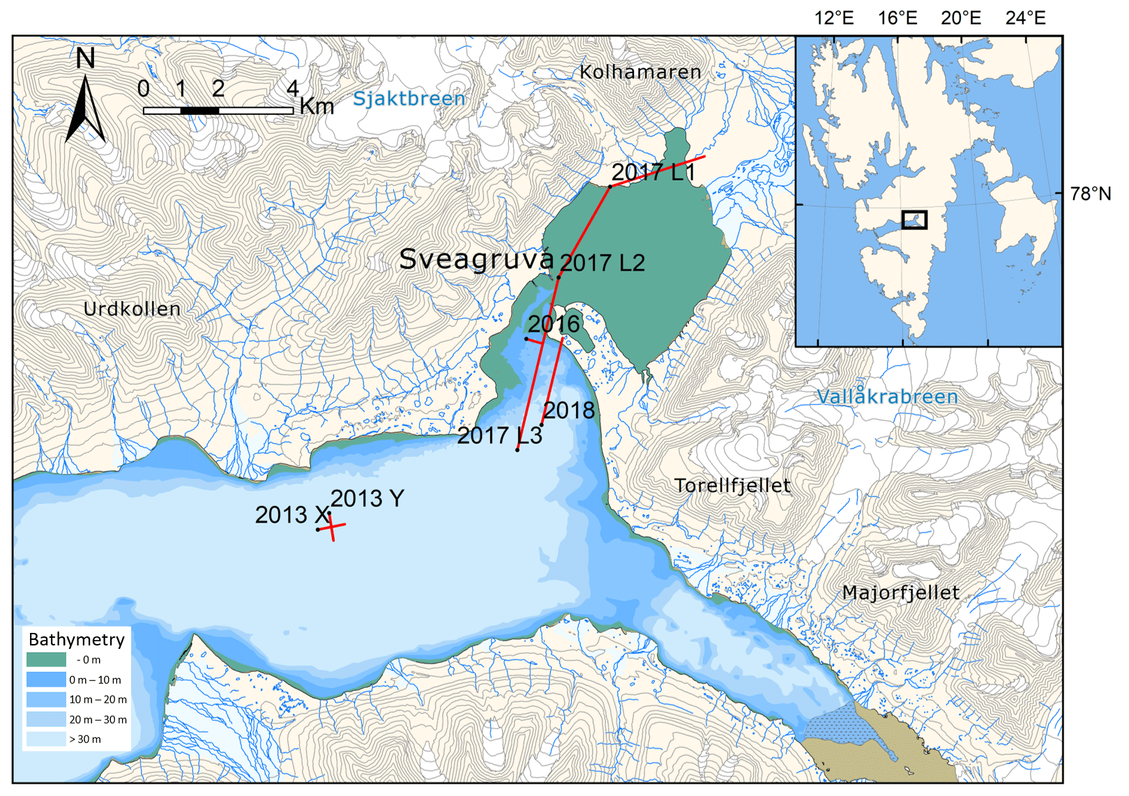
Figure 1 A 1 : 100 000 scale map of the innermost part of Van Mijenfjorden, Spitsbergen, showing the geophone arrays (red lines) deployed during field campaigns in 2013, 2016, 2017 and 2018. Inset map indicates the position relative to the Svalbard archipelago. Land contour interval is 50 m. Map data © Norwegian Polar Institute (https://npolar.no, last access: 25 June 2020).

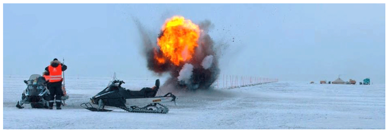
Figure 2 Photo taken during the 2013 field campaign showing the explosive seismic source. The line of seismic receivers is marked with red poles (photo: Robert Pfau).

3 Theory

3.1 General wave field solution

In this study we approximate the air–ice–water system by a thin elastic plate resting on an incompressible inviscid fluid of finite depth, H, that corresponds to the widely used “simplest acceptable” mathematical model advocated by Squire et al. (1996). The plate extends infinitely along the horizontal x and y axes, and the vertical axis, z, is positive downwards with its origin at the upper undisturbed water surface. We impose the constraint that the fluid must satisfy the Laplace equation, ∇²ϕ=0, where ϕ is the velocity potential in the fluid. In addition, we impose a non-cavitation condition at the ice–water interface, ${\left.\frac{\partial \mathit{\varphi }}{\partial z}\right|}_{z=b}=\frac{\partial \mathit{\zeta }}{\partial t}$, where b is the draught of the ice and a normal flow condition at the sea bottom, ${\left.\frac{\partial \mathit{\varphi }}{\partial z}\right|}_{z=H}=\mathrm{0}$, where $\mathit{\zeta }\left(x,y,t\right)$ is the vertical deflection of the plate's neutral surface. The linear spatio-temporal dynamics of the system is described by the partial differential equation (e.g. Squire et al., 1996)

$$\begin{array}{}\text{(1)}& D{\mathrm{\nabla }}^{\mathrm{4}}\mathit{\zeta }+{\mathit{\rho }}_{\mathrm{l}}h{\displaystyle \frac{{\partial }^{\mathrm{2}}\mathit{\zeta }}{\partial t^{\mathrm{2}}}}+{\mathit{\rho }}_{\mathrm{w}}g\mathit{\zeta }=-{\mathit{\rho }}_{\mathrm{w}}{\left.{\displaystyle \frac{\partial \mathit{\varphi }}{\partial t}}\right|}_{z=b}-f(x,y,t).\end{array}$$

Here, $D=\frac{E{h}^{\mathrm{3}}}{\mathrm{12}\left(\mathrm{1}-{\mathit{\sigma }}^{\mathrm{2}}\right)}$ is the plate flexural stiffness, E is Young's modulus, h is the plate thickness, σ is Poisson's ratio, ρ_w is the water density, ρ_l is the plate density, g=9.81 m s⁻² is the acceleration due to gravity, and $f(x,y,t)$ is the applied external spatio-temporal force. The solution to Eq. (1) gives useful insight into the dynamics of the air-coupled flexural wave, and an illustrative example is given in Sect. 5.1.

In order to solve for the spatio-temporal deflection of the ice surface, we apply the three-dimensional Fourier transform (FT), defined as

$$\begin{array}{}\text{(2)}& P\left(k_x,k_y,\mathit{\omega }\right)=\int \int \int p\left(x,y,t\right)e^{i\left(k_{x}x+k_{y}y-\mathit{\omega }t\right)}\mathrm{d}x\mathrm{d}y\mathrm{d}t,\end{array}$$

for an arbitrary spatio-temporal function $p\left(x,y,t\right)$. The wave number vector $\mathit{k}=\left[\begin{array}{c}{k}_x\\ k_y\end{array}\right]$ is decomposed in the x and y directions, $k^{\mathrm{2}}={\left|\mathit{k}\right|}^{\mathrm{2}}=k_x^{\mathrm{2}}+k_y^{\mathrm{2}}$, and i denotes the imaginary unit. By applying the FT defined in Eq. (2) to the spatio-temporal fields in Eq. (1), we find that the solution for the deflection in Fourier space is given by

$$\begin{array}{}\text{(3)}& Z\left(k_x,k_y,\mathit{\omega }\right)=-{\displaystyle \frac{F\left(k_x,k_y,\mathit{\omega }\right)}{G\left(k_x,k_y,\mathit{\omega }\right)}},\end{array}$$

where $G\left(k_x,k_y,\mathit{\omega }\right)=D{k}^{\mathrm{4}}+{\mathit{\rho }}_{\mathrm{w}}g-{\mathit{\rho }}_{\mathrm{l}}h{\mathit{\omega }}^{\mathrm{2}}-\left(\frac{{\mathit{\rho }}_{\mathrm{w}}{\mathit{\omega }}^{\mathrm{2}}}{k}\right)\coth \left(kH\right)$. Recalling linear filter theory, the form of Eq. (3) highlights that the floating ice plate simply acts as a linear filter on an arbitrary spatio-temporal input signal. This formulation is also attractive because the physical significance of the different terms in the denominator are clearly preserved: Dk⁴ expresses the bending forces in the plate, ρ_wg is due to the plate buoyancy, ρ_lhω² is the plate acceleration, and $\left(\frac{{\mathit{\rho }}_{\mathrm{w}}{\mathit{\omega }}^{\mathrm{2}}}{k}\right)\coth \left(kH\right)$ arises due to the constraint of finite water depth.

The general solution for the resulting spatio-temporal deflection wave field, $\mathit{\zeta }\left(x,y,t\right)$, is then given by the full three-dimensional inverse FT of $Z\left(k_x,k_y,\mathit{\omega }\right)$ as

$$\begin{array}{}\text{(4)}& \begin{array}{rl}\mathit{\zeta }\left(x,y,t\right)& =-{\displaystyle \frac{\mathrm{1}}{{\left(\mathrm{2}\mathit{\pi }\right)}^{\mathrm{3}}}}\int \int \int {\displaystyle \frac{F\left(k_x,k_y,\mathit{\omega }\right)}{G\left(k_x,k_y,\mathit{\omega }\right)}}\\ & \cdot e^{-i\left(k_{x}x+k_{y}y-\mathit{\omega }t\right)}\mathrm{d}{k}_x\mathrm{d}{k}_y\mathrm{d}\mathit{\omega }.\end{array}\end{array}$$

3.2 Ring delta function source for radial symmetry

To exploit spatial symmetry and reduce the dimensionality of the problem, we approximate the explosive source as a ring-shaped Dirac delta pulse expanding outwards from the origin with radial symmetry. This allows us to reduce the spatial dimensionality of the problem by using the radial coordinate $r=\sqrt{x^{\mathrm{2}}+y^{\mathrm{2}}}$ and representing the propagating air wave source using the ring delta function,

$$\begin{array}{}\text{(5)}& f\left(r,t\right)=-{\displaystyle \frac{\mathrm{1}}{\mathrm{2}\mathit{\pi }r}}\mathit{\delta }\left(r-c_{\mathrm{air}}t\right),\end{array}$$

where c_air is the speed of sound in air. By performing a partial Fourier transform of Eq. (5) with respect to time, t, we obtain the spatio-frequency representation of the source as

$$\begin{array}{}\text{(6)}& F\left(r,\mathit{\omega }\right)=\underset{-\mathrm{\infty }}{\overset{\mathrm{\infty }}{\int }}f\left(r,t\right)e^{-i\mathit{\omega }t}\mathrm{d}t=-{\displaystyle \frac{\mathrm{1}}{\mathrm{2}\mathit{\pi }r{c}_{\mathrm{air}}}}{e}^{-i\mathit{\omega }r/c_{\mathrm{air}}},\end{array}$$

so the spatio-frequency deflection wave field can be written as

$$\begin{array}{}\text{(7)}& Z\left(r,\mathit{\omega }\right)=-{\displaystyle \frac{F\left(r,\mathit{\omega }\right)}{G_{\mathrm{0}}\left(\mathit{\omega }\right)}},\end{array}$$

where

$$\begin{array}{}\text{(8)}& \begin{array}{rl}{G}_{\mathrm{0}}\left(\mathit{\omega }\right)& =D{\left({\displaystyle \frac{\mathit{\omega }}{c_{\mathrm{air}}}}\right)}^{\mathrm{4}}+{\mathit{\rho }}_{\mathrm{w}}g-{\mathit{\rho }}_{\mathrm{l}}h{\mathit{\omega }}^{\mathrm{2}}\\ & -\left(c_{\mathrm{air}}{\mathit{\rho }}_{\mathrm{w}}\mathit{\omega }\right)\coth \left({\displaystyle \frac{\mathit{\omega }H}{c_{\mathrm{air}}}}\right).\end{array}\end{array}$$

The spatio-temporal deflection wave field in radial coordinates then becomes

$$\begin{array}{}\text{(9)}& \mathit{\zeta }\left(r,t\right)=-{\displaystyle \frac{\mathrm{1}}{\mathrm{2}\mathit{\pi }}}\underset{-\mathrm{\infty }}{\overset{\mathrm{\infty }}{\int }}{\displaystyle \frac{F\left(r,\mathit{\omega }\right)}{G_{\mathrm{0}}\left(\mathit{\omega }\right)}}{e}^{i\mathit{\omega }t}\mathrm{d}\mathit{\omega }.\end{array}$$

When evaluating Eq. (9) numerically, we substitute $G_{\mathrm{0}}\left(\mathit{\omega }\right)\to G_{\mathrm{0}}\left(\mathit{\omega }+i\mathit{\gamma }\right)$, where γ>0, which avoids dividing by zero and gives a tuneable heuristic damping parameter for wave attenuation and dissipation.

3.3 Dispersion relation

The dispersion relation for the propagating wave field in the ice sheet is given by the wavenumber and frequency pairs that satisfy the equation

$$\begin{array}{}\text{(10)}& G\left(k,\mathit{\omega }\right)=\mathrm{0}.\end{array}$$

The solution of Eq. (10) gives the general dispersion relation (e.g. Squire et al., 1996)

$$\begin{array}{}\text{(11)}& {\mathit{\omega }}^{\mathrm{2}}={\displaystyle \frac{\left(D{k}^{\mathrm{5}}/{\mathit{\rho }}_{\mathrm{w}}\right)+gk}{kh\frac{{\mathit{\rho }}_{\mathrm{l}}}{{\mathit{\rho }}_{\mathrm{w}}}+\coth \left(kH\right)}}.\end{array}$$

This dispersion relation is complete in the sense that it retains all physical mechanisms included in the dynamical model Eq. (1), and it is well known from previous studies (e.g. Greenhill, 1886; Squire et al., 1996). At typical vehicle speeds and wavelengths that have been the main focus of moving load on floating plate studies, the plate acceleration may be safely neglected (e.g. Schulkes and Sneyd, 1988; Wang et al., 2004) giving the approximate dispersion relation

$$\begin{array}{}\text{(12)}& {\mathit{\omega }}^{\mathrm{2}}\approx \left({\displaystyle \frac{D{k}^{\mathrm{4}}}{{\mathit{\rho }}_{\mathrm{w}}g}}+\mathrm{1}\right)gk\tanh \left(kH\right).\end{array}$$

Another common assumption is to assume infinite water depth, H, which causes the hyperbolic tangent term to approach unity. However, when the load moves at the speed of sound in air, plate flexural waves with much shorter wavelengths are resonant, and it becomes important to retain the plate acceleration term. The common approximations that are valid at typical vehicle speeds may lead to significant inaccuracies when estimating physical properties of the floating ice sheet from estimates of air-coupled flexural wave frequency.

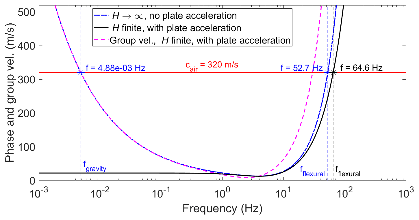
Figure 3 Comparison of simplified dispersion relation neglecting water depth and plate acceleration (blue, Eq. 12) with the full dispersion relation including these effects (black, Eq. 11) for h=0.74 m and sea ice physical properties from Table 1.

Figure 3 compares the full dispersion relation (Eq. 11) with the approximation that neglects water depth and plate acceleration (Eq. 12). Air-coupled waves are excited when the phase velocity is equal to the speed of sound in air, shown as the horizontal red line in Fig. 3. With finite water depth H (black line in Fig. 3), we see that only flexural waves are coupled to the air wave. Gravity waves have been observed in landfast sea ice (Sutherland and Rabault, 2016) and may theoretically couple to the air wave for the case of an infinite fluid (dashed blue line in Fig. 3), but the coupled wave is likely unobservable in practice. The air-coupled flexural waves arrive in advance of the air wave because the group velocity, $\partial \mathit{\omega }/\partial k$, is larger than the phase velocity for a given frequency (dashed magenta line in Fig. 3). The air-coupled flexural frequency is insensitive to water depths >3.2 m, in this example, but is significantly affected by the plate acceleration term. Including the effect of plate acceleration increases the air-coupled flexural frequency by ∼ 23 % using physical properties relevant to our field data (see Table 1). While studies of moving vehicles on floating plates may safely ignore the effect of plate acceleration, we show that it is important to include it when the considered load is moving at the speed of sound in air.

4 Methodology

A key attraction of air-coupled flexural waves is the ability to use the time series recorded by a single sensor to estimate ice thickness. This is possible because, as illustrated by our dynamical model, the phase velocity of the air-coupled flexural wave is equal to the speed of sound in air. This is similar to studies of ice roads and runways, in which the fact that the speed of the vehicle is known raises the potential for routine monitoring of ice flexural rigidity using a single sensor (Squire et al., 1988). The frequency of the air-coupled flexural wave is estimated from the high amplitude, monochromatic segment of the time series that directly precedes the air wave arrival. The air-coupled flexural frequency can then be directly related to the physical properties of the floating ice sheet using the dispersion relation introduced in the previous section.

4.1 Air wave arrival and velocity estimation

Since the arrival time of the air wave increases linearly with horizontal offset between the seismic source and receiver, we can estimate its arrival time and velocity using the linear Radon transform, also referred to as the slant-stack or τ-p transform (Yilmaz, 2001). When the independent variable is source-to-receiver offset, energy with a constant velocity follows a linear trajectory. Under the linear Radon transform, energy corresponding to a specific velocity and origin time is stacked along this trajectory to form a single point in the transform space. For a given explosive charge (see Fig. 4a), we compute the linear Radon transform for offset-sorted geophone signals and estimate the velocity (c_air) and intercept (t_int) that correspond to the air wave by picking the local maximum of the transform magnitude (see Fig. 4b). The estimated arrival time of the air wave at a given geophone, t_air, is then given by $t_{\mathrm{air}}=\frac{d}{C_{\mathrm{air}}}+t_{\mathrm{int}}$, where d is the source-to-receiver offset.

4.2 Thomson multitaper estimation of air-coupled flexural frequency

The frequency of the air-coupled flexural wave is estimated from segments of the recorded time series which precede the arrival of the air wave (see Fig. 4c). We take the derivative of the time series to suppress low frequencies and linearly increase the gain of high frequencies and apply a Hamming window taper. For each time series, the Thomson multitaper power spectral density (Thomson, 1982) is then estimated using a time-half-bandwidth product of 2 and a zero-padded Fourier transform length of 4096 samples. Thomson's estimator utilizes a set of orthonormal data tapers called discrete prolate spheroidal sequences to control spectral leakage and stabilize the estimate through an inherent variance reduction (Hanssen, 1997). The air-coupled flexural frequency (see Fig. 4d) is then estimated from the multitaper power spectral density maximum. We only estimate the air-coupled flexural frequency for source-to-receiver offsets > 125 m because higher-velocity sub-seabed reflections arrive around the same time as the air wave and create too much interference at nearer offsets (see Fig. 5).

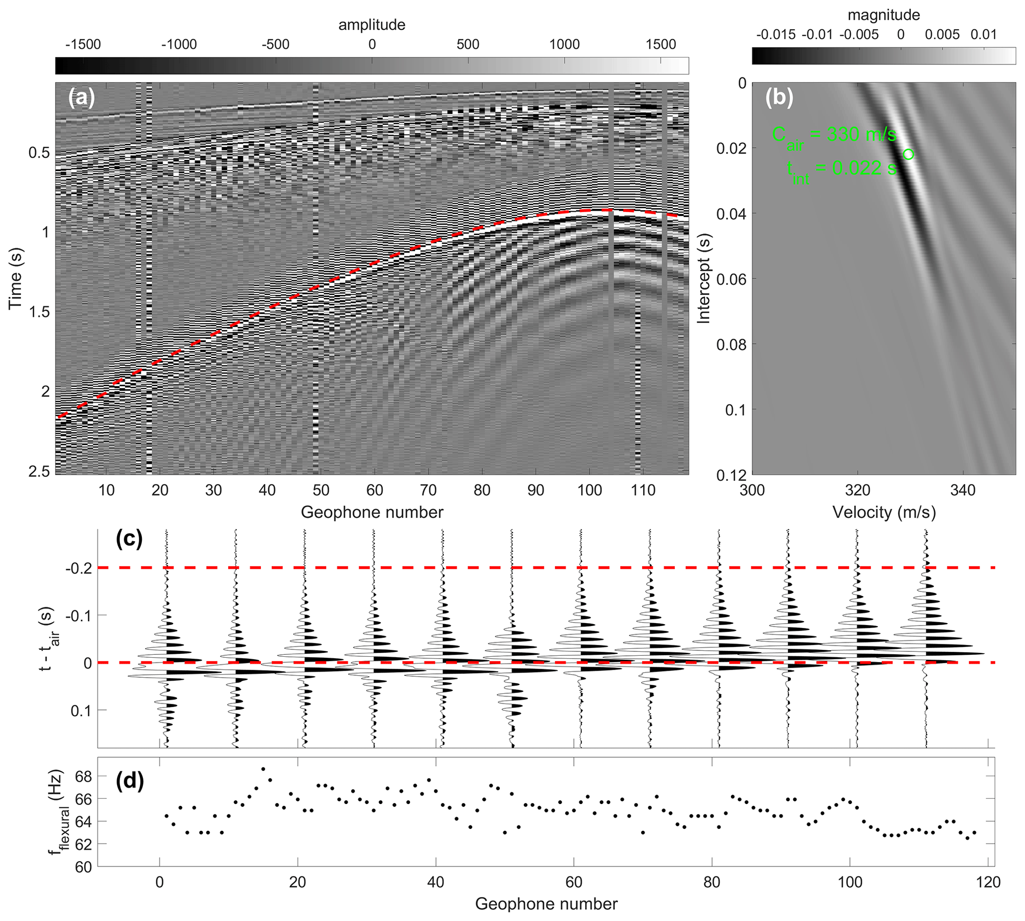
Figure 4 Example of air-coupled flexural wave frequency estimation. (a) Geophone records with dashed red line indicating the air wave arrival, (b) air wave arrival time and velocity is estimated by picking the local maximum of the linear radon transform, (c) waveform plot for every 10th geophone indicating the frequency estimation window (dashed red lines), and (d) air-coupled flexural frequency estimated by the multitaper method.

4.3 Closed-form estimator of ice thickness

Once we have estimated the frequency of the air-coupled flexural wave (ω_f) we can estimate the ice thickness using the dispersion relation (Eq. 11) rearranged as

$$\begin{array}{}\text{(13)}& {\displaystyle \frac{E{h}^{\mathrm{3}}{k}_{\mathrm{f}}^{\mathrm{5}}}{\mathrm{12}{\mathit{\rho }}_{\mathrm{w}}\left(\mathrm{1}-{\mathit{\sigma }}^{\mathrm{2}}\right)}}+g{k}_{\mathrm{f}}={\mathit{\omega }}_{\mathrm{f}}^{\mathrm{2}}\left[k_{\mathrm{f}}h{\displaystyle \frac{{\mathit{\rho }}_{\mathrm{l}}}{{\mathit{\rho }}_{\mathrm{w}}}}+\coth \left(k_{\mathrm{f}}H\right)\right],\end{array}$$

where $k_{\mathrm{f}}={\mathit{\omega }}_{\mathrm{f}}/c_{\mathrm{air}}$ is the wavenumber corresponding to the air-coupled flexural wave. The inclusion of the plate acceleration term means that we are left with a non-linear relation for the plate thickness, h, in terms of the plate elastic properties and the constant flexural frequency and wavenumber. We may either estimate the ice thickness by the non-linear numerical optimization of Eq. (13), using, for example, the bisection method, or we may rearrange Eq. (13) to give the cubic polynomial form

$$\begin{array}{}\text{(14)}& \begin{array}{rl}& \left({\displaystyle \frac{E{k}_{\mathrm{f}}^{\mathrm{5}}}{\mathrm{12}{\mathit{\rho }}_{\mathrm{w}}\left(\mathrm{1}-{\mathit{\sigma }}^{\mathrm{2}}\right)}}\right)h^{\mathrm{3}}-\left({\mathit{\omega }}_{\mathrm{f}}^{\mathrm{2}}{k}_{\mathrm{f}}{\displaystyle \frac{{\mathit{\rho }}_{\mathrm{l}}}{{\mathit{\rho }}_{\mathrm{w}}}}\right)h+g{k}_{\mathrm{f}}\\ & -{\mathit{\omega }}_{\mathrm{f}}^{\mathrm{2}}\coth \left(k_{\mathrm{f}}H\right)=\mathrm{0},\end{array}\end{array}$$

which has one real, positive root corresponding to the plate thickness, h. Since Eq. (14) has a standard cubic form, a closed-form analytical solution can be derived. We followed the modified Cardan's solution method outlined by Nickalls (1993) to derive the following estimator,

$$\begin{array}{}\text{(15)}& h=\mathrm{2}\sqrt{{\displaystyle \frac{b}{\mathrm{3}a}}}\cos \left[{\displaystyle \frac{\mathrm{1}}{\mathrm{3}}}{\cos }^{-\mathrm{1}}\left({\displaystyle \frac{-\mathrm{3}\sqrt{\mathrm{3}}}{\mathrm{2}}}{a}^{\mathrm{1}/\mathrm{2}}{b}^{-\mathrm{3}/\mathrm{2}}c\right)\right],\end{array}$$

where $a=\frac{E{k}_{\mathrm{f}}^{\mathrm{5}}}{\mathrm{12}{\mathit{\rho }}_{\mathrm{w}}\left(\mathrm{1}-{\mathit{\sigma }}^{\mathrm{2}}\right)}$, $b={\mathit{\omega }}_{\mathrm{f}}^{\mathrm{2}}{k}_{\mathrm{f}}\frac{{\mathit{\rho }}_{\mathrm{l}}}{{\mathit{\rho }}_{\mathrm{w}}}$ and $c=g{k}_{\mathrm{f}}-{\mathit{\omega }}_{\mathrm{f}}^{\mathrm{2}}\coth \left(k_{\mathrm{f}}H\right)$. We have confirmed that non-linear numerical optimization of Eq. (13), polynomial root finding of Eq. (14) and the closed form of Eq. (15) all give identical results.

5 Results

Air-coupled flexural waves appear to be a robust part of the wave field excited by explosive sources on floating sea ice and were observed for all four field campaigns, in spite of thin, variable snow covers. Furthermore, Fig. 5 illustrates that since the air-coupled flexural wave precedes the arrival of the air wave, it is recorded equally well for both point and line sources. This is significant because much of our field data employed line sources in order to attenuate the trailing low-frequency ice flexural waves that are an unwanted noise component from the perspective of reflection seismic surveying (Johansen et al., 2019).

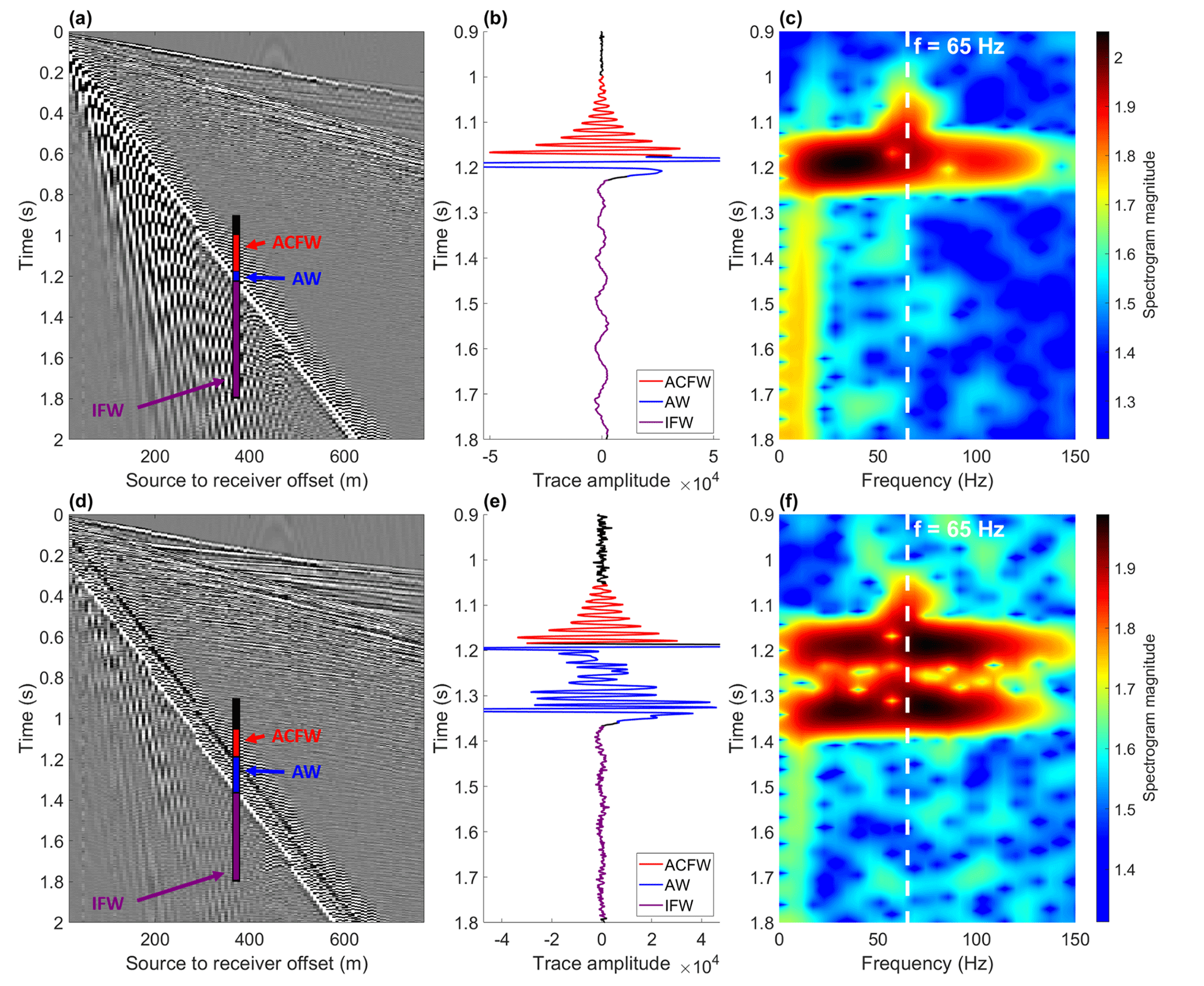
Figure 5 Example geophone records for (a) a point charge and (d) a 50 m long detonating cord line source, (b) and (e) show illustrative time series enlarged around the air wave (AW) arrival, and (c) and (f) show spectrograms for the time series (b) and (e). The air-coupled flexural wave (ACFW) arrives with a constant frequency of ∼ 65 Hz in advance of the broadband air wave. The characteristically dispersive ice flexural waves (IFWs) are significantly attenuated due to destructive interference for the line source.

5.1 Solution of the full dynamical model

It is only strictly necessary to consider the solution to the dispersion relation in order to estimate ice properties from flexural wave observations. However, it is also beneficial to consider the solution to the dynamical equation (Eq. 1) in order to demonstrate that the key physics involved in the propagation of air-coupled flexural waves are represented by the model. To this end, we evaluated Eq. (9) numerically using an inverse fast Fourier transform (IFFT) with N=2¹⁹ discrete points, a temporal sampling interval, $\mathrm{d}t=\mathrm{2.5}\times {\mathrm{10}}^{-\mathrm{4}}$ s, and a numerical attenuation/damping parameter, γ=25. Figure 6 shows a portion of the modelled radially symmetric expanding wave field produced by a propagating ring delta loading that we use as an approximation of the air wave expanding outwards from a point explosive charge and pushing downwards on the ice sheet. We see that the ice sheet is deflected downwards underneath and behind the air wave. The negative deflection decays smoothly and extends to a position around 300 m behind the load, although this is outside the figure view. Ahead of the air wave, the ice surface is elevated, and we see a high amplitude, constant frequency wave train that corresponds to the air-coupled flexural wave, which decays gradually with distance ahead of the load due to the inclusion of numerical damping in the model.

Figure 6 Modelled normalized displacement wave field for h=74 cm, c_air=321 m s⁻¹ and elastic parameters as in Table 1. The black line marks the position of the load (representing the air wave).

To compare the solutions of the full dynamical model result with field data, we calculate the velocity response of the plate at a given offset by numerical time differentiation of the output from Eq. (9) and compare that directly to the recorded geophone time series at the same offset. We find that local velocity estimates calculated from our solutions to the dynamical model are very similar to the real waveforms recorded by geophones, as illustrated by the example in Fig. 7. This increases our confidence that we understand the underlying physics that describe the excitation of air-coupled flexural waves in floating ice sheets.

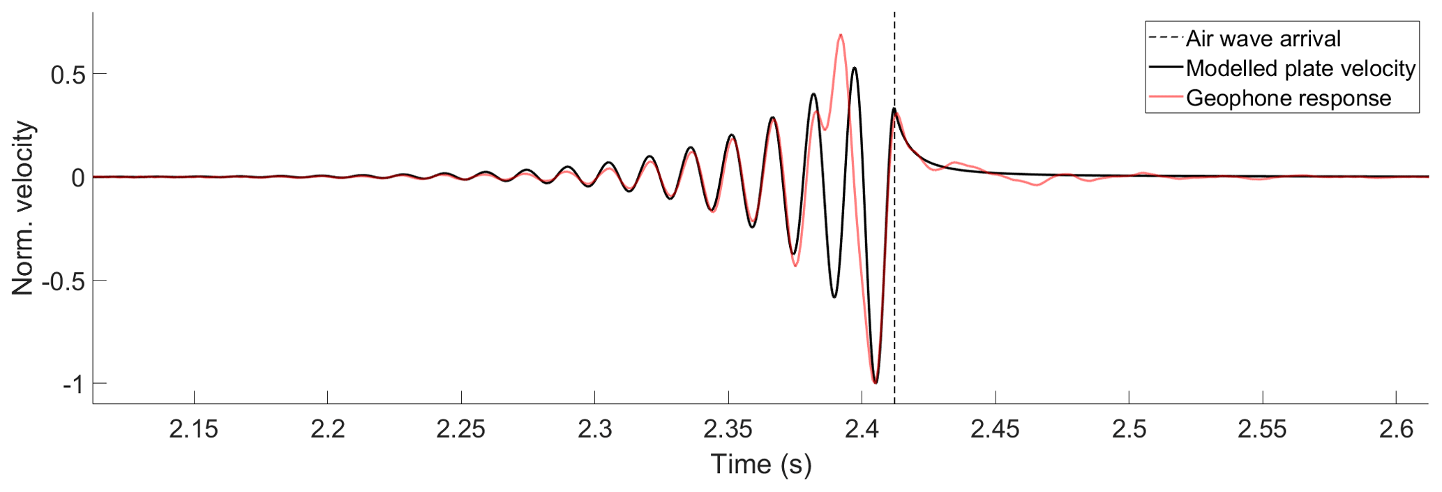
Figure 7 Modelled normalized velocity response time series (black curve) at an offset of 759 m compared with the time series recorded by a geophone at the same offset from a point charge fired during the 2013 field season (red curve). The air wave arrival time is indicated by the dashed line.

5.2 Ice thickness estimation from air-coupled flexural waves

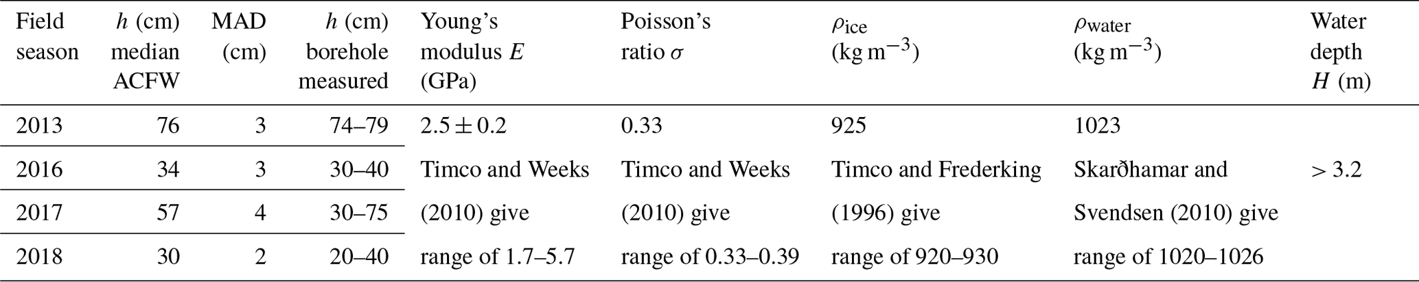
As summarized in Table 1, ice thicknesses calculated using Eq. (15) from the estimated air-coupled flexural frequencies and air wave velocities show very good agreement with ice thicknesses measured in boreholes. Notably, this good agreement was achieved across all four field seasons with a single set of elastic properties that are realistic for sea ice. This is partly because ice thickness is an extrinsic property that has a dominant effect on the air-coupled flexural frequency (stemming from the fact that D∝h³); i.e., the 20–80 cm thickness range from this study corresponds to a 400 % variation in air-coupled flexural frequency. By contrast, variation of intrinsic material properties, i.e., Young's modulus (1.7–5.7 GPa) and Poisson's ratio (0.33–0.39) as reported by Timco and Weeks (2010), for first-year sea ice would give ∼ 60 % and ∼ 2 % variation in air-coupled flexural frequency, respectively. The combined effects of water and ice density variation over the ranges given in Table 1 would only produce a variation of ∼ 0.3 % in air-coupled flexural frequency, while water depth has no effect for depths >3.2 m. Temperature variation over the range −20 to +2 ^∘C would cause the speed of sound in air to vary from 318–332 m s⁻¹, resulting in ∼ 8 % variation in air-coupled flexural frequency. The apparent speed of sound in air at the measurement location is also affected by horizontal wind velocity, and gusts may lead to a variation of ±5 m s⁻¹ over timescales of minutes (e.g. Franke and Swenson, 1989). However, as described in Sect. 4.1, we estimate the apparent velocity of the air wave for each shot, which should ensure that our air-coupled flexural thickness estimates are independent of changes in wind and temperature over time.

The Young's modulus of 2.5±0.2 GPa given in Table 1 was constrained by observing that the median air-coupled flexural wave thickness estimate for the 2013 field season would fall outside the range of borehole-measured thicknesses for Young's modulus outside this range. The fact that this Young's modulus gives thickness estimates that fit with borehole measurements across all four field seasons indicates that the bulk, effective elastic properties of first-year sea ice in Van Mijenfjorden are relatively consistent from year to year. A somewhat higher Young's modulus of ∼ 4 GPa was reported for Van Mijenfjorden by Moreau et al. (2020a), but the deviation from the present study is likely attributable to the protected physical setting of their study site at the estuarine Vallunden lake. It is also important to highlight that all elastic properties we assume represent bulk, apparent values corresponding to the thin isotropic plate assumption, while real floating ice sheets are a composite sandwich material consisting of multiple ice layers of varying strength (Timco and Weeks, 2010).

Table 1 Summary of ice thicknesses (h) estimated from air-coupled flexural waves (ACFW) compared to the range of ice thicknesses measured in boreholes drilled through the ice. MAD signifies median absolute deviation.

Here we give a summary of our air-coupled flexural wave ice thickness estimates for each field season and examine them in the context of borehole measurements of ice thickness and prevailing meteorological conditions, as represented by records at the nearby Sveagruva weather station (Norwegian Meteorological Institute, 2020), which was upgraded prior to the 2017 season to include measurement of precipitation. We assume the air-coupled flexural frequency recorded at a given geophone is related to the ice thickness at the location of the geophone as this gave the strongest correlation with borehole thickness measurements.

5.2.1 The 2013 field season

The ice thickness estimates for the 2013 field season are summarized in Fig. 8 and show good agreement with borehole measurements. There is somewhat greater spread in the results on the Y line which is likely related to the fact that the majority of the source positions were inline with the X line and therefore oblique to the Y line (see Fig. 1). The oblique geometry reduces the precision of using the linear Radon transform to estimate the arrival time and velocity of the air wave, which becomes smeared in the transform domain. Air temperatures remained consistently <0 ^∘C, and the thickness estimates are quite similar over the ∼ 3 d field campaign, though there is some indication of ice growth with time.

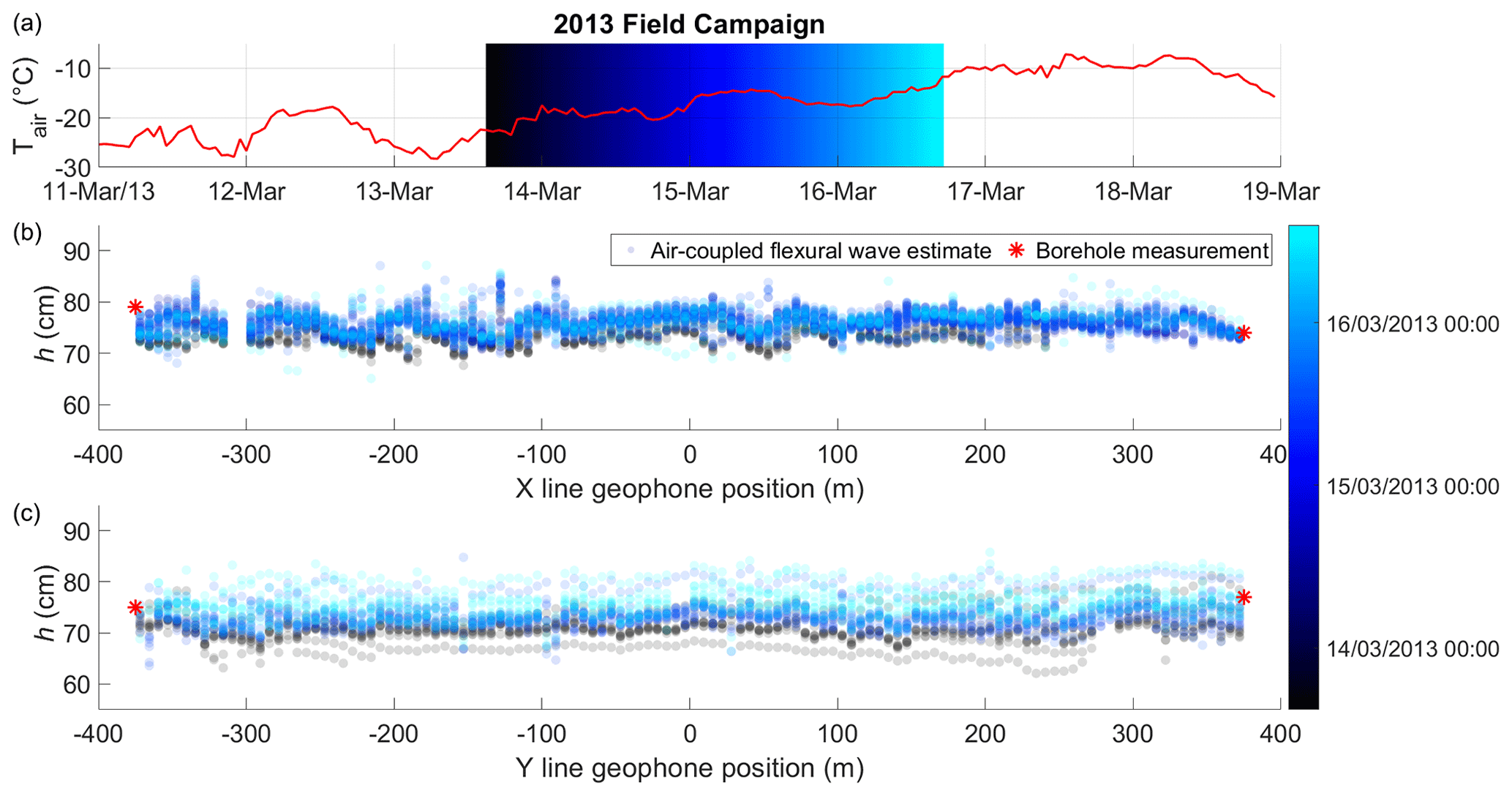
Figure 8 The 2013 field campaign air-coupled flexural wave ice thickness estimates (circles), borehole drilled thicknesses (red stars) and air temperature at nearby Sveagruva weather station (red line). The time span of the field campaign is indicated by black–blue–cyan colour gradient. Point estimates are transparent so overlapping repeat tests are indicated by denser colours. Figure 1 shows location of the profiles 2013 X (b) and 2013 Y (c).

5.2.2 The 2016 field season

The results for the 2016 field season are illustrated in Fig. 9. Some outliers are present in the flexural wave thickness estimates which are caused by interference of other spectral components for the extracted time series segments. This interference can be due to, for example, other wave modes such as sub-seabed reflections, snow scooter engine noises or instrument noise due to wind. Despite these outliers, the median thickness estimates agree well with the range of drilled thicknesses (see Table 1), although the along-profile locations of the boreholes was unfortunately not recorded for this field campaign.

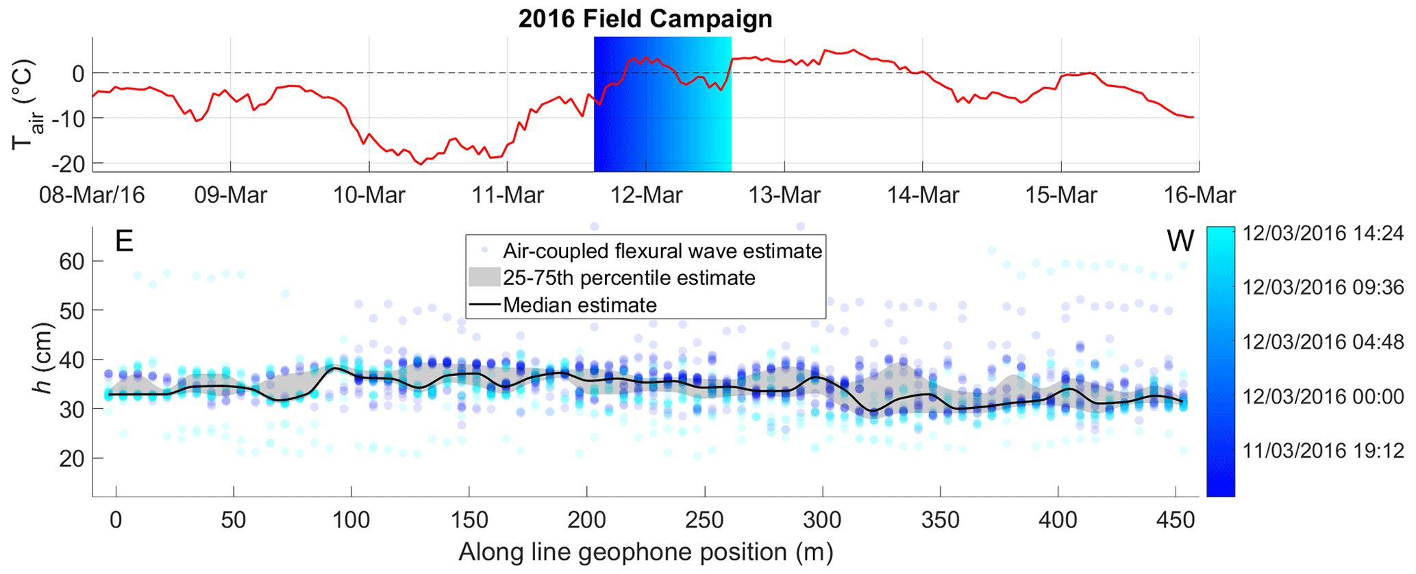
Figure 9 The 2016 field campaign air-coupled flexural wave ice thickness estimates (circles) and temperature at nearby Sveagruva weather station (red line). Time span of field campaign is indicated by blue–cyan colour gradient. Point estimates are transparent so overlapping repeat tests are indicated by denser colours. Figure 1 shows location of profile.

5.2.3 The 2017 field season

The thickness estimates for the 2017 field season are shown in Fig. 10. The significant spatial thickness variation observed in boreholes is reasonably well represented by the median air-coupled flexural wave thickness estimates plotted according to geophone position, though the estimates vary more smoothly in space. This indicates that the air-coupled flexural wave varies according to the thickness and flexural rigidity of the ice in the vicinity of the geophone, likely averaged spatially in proportion with the wavelength of flexure. An alternative hypothesis that the air-coupled flexural wave is controlled by the path-averaged ice properties between the source and geophone was tested by plotting the thickness estimates at the midpoint between source and receiver. While we do not include the figure for brevity, the result is a flat profile with estimates ranging from ∼ 45–75 cm and a similar median of ∼ 57 cm. This does not reflect the real thickness variation recorded by the borehole measurements, leading us to prefer the hypothesis that the frequency of the air-coupled flexural wave is controlled by the ice thickness and flexural rigidity in the vicinity of the geophone. Indeed, we found the borehole-measured spatial variation in ice thickness could only be approximated by assuming the air-coupled flexural wave estimates lie at least 98 % towards the geophone (along the straight line from source to geophone).

We also observe that the air-coupled flexural wave thickness estimates significantly overestimate the ice thickness drilled in the two boreholes closest to land. While further field data would be needed to investigate this phenomenon in detail, it may be attributable to the effect of the land on the lateral boundary condition of the ice sheet (see Appendix A). The infinite ice sheet modelled in the present study does not include a lateral boundary, though it may be possible to heuristically approximate this effect by defining a spatially variable effective elastic modulus that increases near land.

Figure 10 Profile 2017 L3 from 2017 field campaign, seaward direction is south (see Fig. 1) showing air-coupled flexural wave ice thickness estimates (circles), borehole drilled thicknesses (red stars), temperature (red line) and precipitation (green bars) at Sveagruva weather station. Timing is indicated by black–blue–cyan colour gradient, and point estimates are transparent so overlapping repeat tests are indicated by denser colours.

5.2.4 The 2018 field season

The air-coupled flexural wave thickness estimates for the 2018 field season are summarized in Fig. 11. The thickness estimates agree well with the range of ice thickness measured in boreholes (see Table 1), though the along-profile locations of the boreholes were unfortunately not recorded for this field campaign. The most striking feature we observe for the 2018 campaign is an increase in ice thickness of up to ∼ 10–15 cm over the course of the campaign (a period of ∼ 4 d). This rapid increase in thickness is attributable to the weather event that occurred on 26–27 February, when > 0 ^∘C temperatures and rain led to a significant accumulation of freshwater on top of the sea ice. This event was significant enough that fieldwork was not possible on 27 February. The rapid decrease in air temperature on the 28th then promptly caused the accumulated fresh surface water to freeze, a process that occurs much more quickly than basal ice accumulation due to heat loss through the overlying ice layer, salt rejection and eventual freezing of seawater.

Figure 11 The 2018 field campaign air-coupled flexural wave ice thickness estimates (circles), temperature (red line) and precipitation (green bars) at Sveagruva weather station. Timing of experiments is indicated by blue–cyan colour gradient, and point estimates are transparent so overlapping repeat tests are indicated by denser colours. Figure 1 shows location of profile. Median is shown with a dashed line because there are two distinct, temporally separated populations.

6 Discussion

It is possible to interpret the origin of the air-coupled flexural waves in several equivalent ways. (1) They are produced by the downward pressure of the air wave moving over the ice surface, i.e., the moving loads on floating plates interpretation as elaborated in Sect. 3. (2) A plate excited by a broadband pulse propagates flexural wave energy at a range of frequencies, but sound transmission from the plate is highest at the coincidence frequency (Bhattacharya et al., 1971) producing a resonance effect. (3) Alternatively, the air-coupled flexural wave can be interpreted as a class of leaky Lamb waves in which flexural wave energy radiates into the air, regulated by the phase matching condition and occurring most efficiently at the grazing angle, where the phase velocity is equal to the speed of sound in air (Brower et al., 1979; Kiefer et al., 2019; Mozhaev and Weihnacht, 2002). The observation of air-coupled flexural waves and absence of dispersive ice flexural waves on the far side of open water leads by Hunkins (1960) is consistent with the interpretation that, for explosive sources on or above the ice, air-coupled flexural waves are generated continuously by the downward pressure exerted by the air wave. The correspondence between experimental data and the solution of the full dynamical model (see Fig. 6) gives further support to this interpretation.

Our results indicate that air-coupled flexural waves are affected by spatial (see Fig. 10) and temporal ice thickness variation (see Fig. 11). A high degree of spatial variability in ice thickness has been reported for first-year sea ice in Van Mijenfjorden (Sandven et al., 2010) and in the Arctic in general (Wadhams et al., 2006). Spatial resolution is likely proportional to the air-coupled flexural wavelength, though further field data including high-resolution ground truth measurements would be required to elaborate this proportionality in detail. It is also important to highlight that the air-coupled flexural frequency is affected by the elastic properties of the ice, its flexural rigidity and not just its thickness. By assuming a constant set of elastic parameters our thickness estimates may be considered “effective thicknesses” corresponding to the assumed elastic parameters and subject to the thin isotropic plate assumption. However, we also expect that the “effective thickness” for assumed elastic properties is still highly relevant when assessing the load bearing capacity of floating ice even if it were to deviate from the true thickness.

A small percentage of outliers are present in the thickness estimates that we attribute to spectral contamination caused by the simultaneous arrival of other wave modes with the air-coupled flexural waves. Such interference was minimized by discarding the nearest offsets where high-velocity sub-seabed reflections arrive at the same time as the air wave (see Fig. 5). However, other noise sources, such as snow scooter traffic, are difficult to avoid in real-world data. In the rare cases that traffic noise is recorded at the same instant as the air-coupled flexural waves, the resulting spectral interference can prevent accurate estimation of the air-coupled flexural frequency. Snow cover also likely decreases the efficiency of coupling between ice and air, though this did not appear to play a major role for the four field seasons investigated, for which gimballed z-component geophones were deployed directly on top of the thin snow covers that were present.

Air-coupled flexural wave data acquisition

In this study, we present data acquired with linear arrays of geophones and active seismic sources that were primarily acquired to test the feasibility of seismic reflection surveying on floating sea ice. It is important to emphasize that it should be possible to employ much simpler equipment to record air-coupled flexural waves. Indeed, from our results we would expect that a simple microphone, sensitive in the relevant frequency range and located in the vicinity of the desired measurement, either above the ice sheet or along the shoreline may be sufficient. In addition to low equipment cost, the potential to monitor ice thickness using a microphone positioned on land could be beneficial from the perspective of environmental monitoring, particularly early in the freezing season when the ice is too thin to be safely traversed.

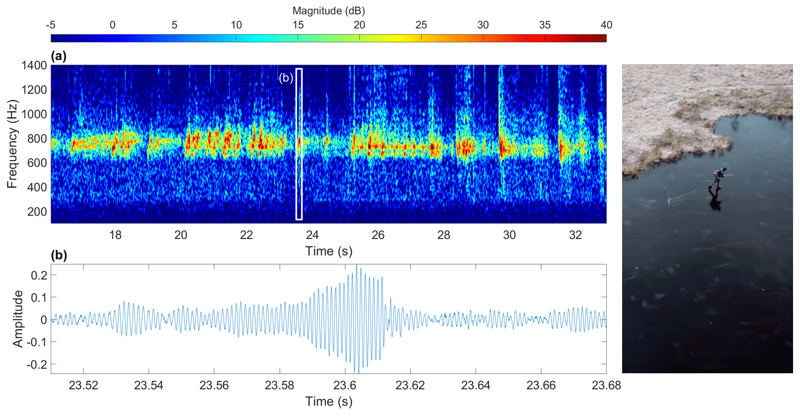
Figure 12 (a) Spectrogram of audio track from 16 s to 33 s of the National Geographic short film “How Skating on Thin Ice Creates Laser-Like Sounds” (Rankin, 2018) and (b) example of waveform dominated by the monochromatic air-coupled flexural wave and broadband impulse at 23.61 s from skate blade cracking ice. Spectrogram is composed of 2¹² sample (∼ 0.09 s), 90 % overlapping Kaiser windows with shape parameter β=10.

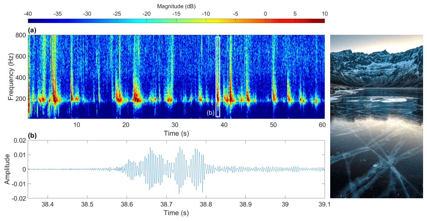
Figure 13 (a) Spectrogram of natural ice quakes at Storvatnet, Kvaløya (Norway), recorded at midday on 3 January 2021 with the built-in microphone of a Sony a6500 camera at a height of ∼ 1.2 m above the ice. Spectrogram is composed of 2¹³ sample (∼ 0.17 s), 90 % overlapping Kaiser windows with shape parameter β=10. The waveform of the strong ∼ 190 Hz monochromatic component corresponding to the air-coupled flexural wave is shown in detail in (b).

The use of microphones to record air-coupled flexural waves can be illustrated by a phenomenon that is familiar to the ice-skating community. On thin, floating ice, skates striking or cracking the ice can excite sonorous tones that vary in pitch according to the ice thickness (Lundmark, 2001). These tones correspond to air-coupled flexural waves, simply shifted to higher frequencies because of the thinner, stiffer freshwater ice. We use the audio track from the well-known National Geographic short film “How Skating on Thin Ice Creates Laser-Like Sounds” (Rankin, 2018) to illustrate this. The frequency of the strong monochromatic component corresponding to the air-coupled flexural wave is ∼ 725 Hz for the scene from 16 s to 33 s, as shown in Fig. 12. Using Eq. (15) we calculate that the ice was ∼ 4.3 cm thick, assuming Young's modulus of 8.5 GPa, Poisson's ratio of 0.33, water density of 1000 kg m⁻³, ice density of 917 kg m⁻³, water depth of at least 0.3 m and sound speed of 329 m s⁻¹ corresponding to an air temperature of −3.9 ^∘C. This is in line with the measured ice thickness presented in the film and illustrates the potential to use air-coupled flexural waves recorded by a simple microphone to estimate ice thickness.

Detonating cord seismic sources were used for the experiments presented in this study, but other impulsive sources acting on a floating ice sheet also have the potential to excite air-coupled flexural waves. Hammer blows are an alternative active source, while crack propagation is a potential passive source that produces a sudden energy release capable of exciting propagating elastic waves in the plate and acoustic pressure waves in air. Ice quakes produced by the sudden cracking of floating ice are a well-known phenomenon (Kavanaugh et al., 2019; Moreau et al., 2020b; Olinger et al., 2019; Ruzhich et al., 2009) and are typically related to the build-up of stress by thermal, tidal and wind forces. This phenomenon has also been studied from the structural non-destructive testing perspective, for example, by Haider and Giurgiutiu (2018) who model the acoustic emission of axis-symmetric circular crested Lamb waves excited by crack propagation in a steel plate.

In order to illustrate that ice quakes are capable of producing air-coupled flexural waves, we went out and recorded a series of ice quakes around midday, 3 January 2021, at Storvatnet, Kvaløya (Norway), using the built-in microphone of a Sony a6500 digital camera. This is a relatively low-quality microphone with no shielding from wind noise, but the monochromatic air-coupled flexural waves can still be clearly discerned (in addition to the broadband impulses of the ice crack ruptures). The ice was not drilled, but its thickness was estimated to be 10–20 cm by visual assessment of vertical cracks running through the clear, black ice. The air-coupled flexural frequency of ∼ 195 Hz indicates the thickness was 16 cm, using the same physical properties for lake ice as introduced earlier. The midday occurrence of these ice quakes, when air temperature was relatively high, suggests they were caused by thermal expansion stresses (Ruzhich et al., 2009). The results of this study and the examples shown in Figs. 12 and 13 suggest that the non-contact, passive recording of air-coupled flexural waves using a single microphone may provide an additional, alternative method of passive flexural wave ice thickness estimation. This complements previously demonstrated passive seismic monitoring methods employing array-based wave field transform approaches (Moreau et al., 2020a) or noise interferometry and Bayesian inversion (Moreau et al., 2020b). The use of inexpensive single, non-contact sensors is an attractive aspect of the air-coupled flexural wave method, particularly the fact that a microphone could be placed on land when the ice is too thin to safely traverse. However, further study is needed to reveal the extent to which the temporal occurrence of ice quakes producing air-coupled flexural waves and reduced air–ice coupling due to thick snow covers may limit the practical acquisition season.

7 Conclusion

Air-coupled flexural waves were found to be a robust feature of first-year sea ice excited by explosive sources over a range of ice thicknesses up to ∼ 80 cm. The physics of these waves can be understood from a theoretical perspective that has largely developed through the study of moving vehicles on floating plates. The dynamical model that we favour is straightforward to understand in terms of linear filter theory, and we derived a closed-form solution of the dispersion relation that relates ice thickness directly to the air-coupled flexural wave frequency and air wave velocity. We tested the proposed closed-form ice thickness estimator extensively on field data from four field seasons and found a remarkably good agreement with in situ borehole measurements. The phenomenon of air-coupled flexural waves is relatively familiar to the wild ice-skating community, in which thin ice produces air-coupled flexural waves that are readily audible. Here we build on the pioneering efforts of Press and Ewing (1951), developing a more accessible theory supported by modern numerical and Fourier transform methods, to show that the same phenomenon also occurs for much thicker sea ice, simply shifted to a lower frequency regime. We have mainly presented data that were acquired for the primary purpose of reflection seismic profiling, but a key benefit of air-coupled flexural waves is that they can also be recorded with very simple equipment, such as a single microphone located either above the ice sheet or along the shoreline. Ice quakes produced by natural cracking excite air-coupled flexural waves for freshwater lake ice, which raises the potential that passive recording of air-coupled flexural waves may also be possible for sea ice.

Appendix A: Possible effect of land on ice sheet lateral boundary condition

Two outlier points were observed for the 2017 field season, in which ice with drilled thickness of 30–35 cm near land had air-coupled flexural frequency similar to ice of 50 cm drilled thickness further seaward (see Fig. 10). To illustrate that this may be attributable to a lateral boundary condition effect, we approximate an ice sheet of finite extent as a collection of arbitrarily small, uniformly loaded, circular plates. The ice along the shoreline is represented by assuming a clamped boundary condition, while the ice far from shore is considered simply supported by the neighbouring plate elements. We may then find the thicknesses of a simply supported and a clamped plate that lead to equal maximum tangential stresses. From Hearn (1997), the maximum tangential stress, occurring at the centre of the simply supported plate, σ_s, and the clamped plate, σ_c, is given by

$${\mathit{\sigma }}_{\mathrm{s}}={\displaystyle \frac{\mathrm{3}q{R}^{\mathrm{2}}}{\mathrm{8}{h}_{\mathrm{s}}^{\mathrm{2}}}}\left(\mathrm{3}+v\right)\text{and}{\mathit{\sigma }}_{\mathrm{c}}={\displaystyle \frac{\mathrm{3}q{R}^{\mathrm{2}}}{\mathrm{8}{h}_{\mathrm{c}}^{\mathrm{2}}}}\left(\mathrm{1}+v\right).$$

Here, q is the uniformly distributed load, R is the plate radius, v is Poisson's ratio, and h_s and h_c are the thicknesses of the simply supported and clamped plates, respectively. Equating the two expressions gives

$${\displaystyle \frac{h_{\mathrm{c}}^{\mathrm{2}}}{h_{\mathrm{s}}^{\mathrm{2}}}}={\displaystyle \frac{\left(\mathrm{1}+v\right)}{\left(\mathrm{3}+v\right)}}$$

so that h_c≈0.63h_s for v=0.33. Therefore, it is anticipated that ice 50 cm thick far from shore will experience the same maximum tangential stress under load as ice that is $\mathrm{0.63}\times \mathrm{50}=\mathrm{32}$ cm thick at the shoreline (consistent with the outlier points from the 2017 field season). We may similarly equate the maximum deflections of the plates, which also occur at the plate centres. Hearn (1997) gives the relevant expressions for the maximum deflection of the plates as

$$w_{\mathrm{s}}={\displaystyle \frac{\mathrm{3}q{R}^{\mathrm{4}}}{\mathrm{16}E{h}_{\mathrm{s}}^{\mathrm{3}}}}\left(\mathrm{5}+v\right)\left(\mathrm{1}-v\right)\text{and}{w}_{\mathrm{c}}={\displaystyle \frac{\mathrm{3}q{R}^{\mathrm{4}}}{\mathrm{16}E{h}_{\mathrm{c}}^{\mathrm{3}}}}\left(\mathrm{1}-v^{\mathrm{2}}\right),$$

where E is the Young's modulus. By equating the two deflections and simplifying we find

$${\displaystyle \frac{h_{\mathrm{c}}^{\mathrm{3}}}{h_{\mathrm{s}}^{\mathrm{3}}}}={\displaystyle \frac{\left(\mathrm{1}-v^{\mathrm{2}}\right)}{\left(\mathrm{5}+v\right)\left(\mathrm{1}-v\right)}},$$

which again gives h_c≈0.63h_s for v=0.33. Since both tangential stress and strain are equal for a clamped plate with 63 % of the thickness of a corresponding simply supported plate, the boundary condition effect can also be understood as a change in effective elastic modulus. This supports the heuristic approximation of the lateral boundary condition effect by a spatially variable, effective elastic modulus. While this theoretical description is simplistic since, for example, the fluid loading is ignored, it highlights that the boundary condition of a finite plate can play a significant role. It would be beneficial to explore this effect in greater detail in future studies, particularly with regard to the length scale involved in the transition from clamped to simply supported behaviour. Accurately describing this behaviour would require the collection of more detailed field data in the zone near the shoreline in order to constrain the development of a more complete model, such as a full finite element simulation.