the Creative Commons Attribution 4.0 License.
the Creative Commons Attribution 4.0 License.
 | 28 Jun 2021
Sensitivity of the Greenland surface mass and energy balance to uncertainties in key model parameters
Andreas Born
We investigate the sensitivity of a distributed glacier surface mass and energy balance model using a variance-based analysis, for two distinct periods of the last glacial cycle: the present day (PD) and the Last Glacial Maximum (LGM). The results can be summarized in three major findings: the sensitivity towards individual model parameters and parameterizations is as variable in space as it is in time. The model is most sensitive to uncertainty related to atmospheric emissivity and the down-welling longwave radiation. While the turbulent latent heat flux has a sizable contribution to the surface mass balance uncertainty in central Greenland today, it dominates over the entire ice sheet during the cold climate of the LGM, in spite of its low impact on the overall surface mass balance of the Greenland ice sheet in the modern climate. We conclude that quantifying the model sensitivity is very helpful for tuning free model parameters because it clarifies the relative importance of individual parameters and highlights interactions between them that need to be considered.
- Article
(7598 KB) - Full-text XML
- BibTeX
- EndNote


Of the many challenges to accurately simulate past variations in the volume of the Greenland ice sheet (GrIS) and to project its future contribution to sea level rise, recent studies agree that the uncertainty associated with surface mass balance (SMB) is among the most important (Aschwanden et al., 2019; Plach et al., 2019).
Models to calculate SMB cover a whole range of complexities from empirical index models that only account for air temperature (Ohmura, 2001; Zemp et al., 2019) or temperature and solar radiation (Bintanja et al., 2002; Van Den Berg et al., 2008; Robinson et al., 2011) to coupled atmosphere–snow models that simulate the snowpack in multiple layers and give a full representation of the atmospheric circulation, based on physical first principles (Lehning et al., 2002; Fettweis, 2007; Noël et al., 2018). On this spectrum, the empirical models perform well for the observational period and when the temperature sensitivity of the SMB is well known (Fettweis et al., 2020), but they are difficult to constrain for temporal and spatial climate variations and become unreliable for conditions outside their relatively narrow tuning interval (van de Berg et al., 2011; Plach et al., 2019). There is a lack of constraint in empirical models even though their low computational requirements make them attractive for the long integration times that are needed to simulate continental ice sheets. Their shortcomings severely limit the usefulness of their results. On the other hand, detailed snow models and especially those coupled with regional atmosphere models are computationally too expensive to run for long periods of time. This situation motivated the development of models that balance the defensible representation of the relevant physical processes with computational efficiency (Krapp et al., 2017; Krebs-Kanzow et al., 2018; Born et al., 2019).
In this study, we use the BErgen Snow SImulator (BESSI), a model that is designed to include all relevant physical mechanisms with reasonable detail but is specifically prepared for long integration times by reducing its computational requirements and by strictly conserving mass and energy (Born et al., 2019). Adding to the original model version, we now include three different parameterizations for snow aging based on Oerlemans and Knapp (1998), Aoki et al. (2003), and Bougamont et al. (2005). The turbulent latent heat flux is now also simulated. For this study the model domain was reduced to Greenland at a resolution of 10 km, but all model changes are also applicable to the original setup.
Multiple studies have investigated the impact of the turbulent latent heat flux on the surface mass balance (Box and Steffen, 2001; Box et al., 2004; van Den Broeke et al., 2008; Cullen et al., 2014; Noël et al., 2018). They find a relatively small impact of the vapor fluxes on the Greenland ice sheet total mass balance (≈ 5 Gt a−1; Cullen et al., 2014), but their local impact can be up to 20 % of the annual accumulation (Box et al., 2004). The importance of the vapor flux is difficult to assess for different climatic settings because, as Box and Steffen (2001) have shown, the choice of the calculation method impacts the results greatly in regions of low mass flux like the dry interior zone of Greenland. This is exacerbated by the fact that turbulent latent heat fluxes are mostly negative in winter under the present climate conditions and positive in summer, so the sign of the net flux may change with a different climate. During the colder climate of the glacial a much larger impact of the turbulent latent heat flux can be assumed, similarly to the much greater importance it currently has in Antarctica (e.g., Gallet et al., 2014; van Wessem et al., 2018). A parameterization based on the bulk method by Rolstad and Oerlemans (2005) has been added to BESSI to simulate the turbulent latent heat flux.
To assess the sensitivity of the new parameterizations and that of BESSI overall, we employ a variance-based approach (Saltelli et al., 2000, 2006, 2010; Sauter and Obleitner, 2015) that has previously been used to quantify the sensitivity of glacier and ice models (Aschwanden et al., 2019; Bulthuis et al., 2019; Zolles et al., 2019). We extend the sensitivity analysis used by Zolles et al. (2019) to provide spatial patterns of sensitivity indices. Following our model's design goal to be used over timescales of glacial cycles and accounting for potentially different sensitivities under different climate boundary conditions, we analyze two large ensembles with a total of 16 500 simulations, for the present-day (PD) climate and for that of the Last Glacial Maximum (LGM). The result is rich information on what parameters and parameterizations have the largest impact on the model's performance and how this sensitivity varies in different regions of Greenland and over time. Knowing the sensitivity also enables a better calibration of the model parameters as the knowledge prevents or reduces over-fitting to a particular study location or time (Beven, 1989).
The revised model is described in Sect. 2. The distributed sensitivity analysis of multiple model output variables in relation to model parameters, including those for the new parameterizations for turbulent latent heat flux and snow aging, is presented in Sect. 3. After that, we discuss our findings in Sect. 4 and conclude in Sect. 5.
The study uses the efficient mass and energy balance model BESSI, which is designed to simulate the mass balance over long timescales (Born et al., 2019). The energy exchange between the snow and the atmosphere is altered in the model version used here, while the subsurface and internal processes are unchanged from the previously published version. The following model was enhanced to include the turbulent latent heat flux and multiple more-complex snow albedo schemes were added. The model description given in the following focuses entirely on the interaction between the snow surface and the atmosphere. For the numerical description and other subsurface processes like firnification and heat conduction, see Born et al. (2019).
The model setup used here has a 10 km grid for the domain of Greenland. The vertical dimension is discretized based on the mass with up to 15 layers in the snowpack (Born et al., 2019). The mass of each layer is 100–500 kg m−2. Each cell has a default maximum of 300 kg m−2, but due to melt and refreezing the mass may decrease or increase, respectively. Cells above 500 kg m−2 or below 100 kg m−2 are split or merged, respectively, to restore the default maximum value. Simulations require daily input of air temperature, total precipitation, and solar radiation and its reference height. Humidity is an optional input which is required if the turbulent latent heat flux is computed. All variables are interpolated to the 10×10 km model grid using bi-linear interpolation. The air temperature is the only meteorological input which is vertically downscaled to the firn model topography using a temperature lapse rate of 6.5 K km−1 for the PD and 8.55 K km−1 for the LGM. The output written by the model may be adjusted by the user, who can select values ranging from daily over monthly to annual timescales. Output variables include surface mass balance; melt of snow; melt of ice; runoff; refreezing; albedo; turbulent latent heat flux; and a mask containing snow, land, ice, and water as well as the 3-dimensional grid values for snow mass, snow density, snow temperature, and liquid water mass.
2.1 Surface energy fluxes
The energy exchange between the surface and the atmosphere comprises five different processes, of which the precipitation and the turbulent latent heat flux (vapor flux) also imply a change in mass: the shortwave radiation (QSW), the longwave/thermal radiation (QLW), the turbulent sensible heat flux (QSH), the turbulent latent heat flux (QL), and the heat flux associated with precipitation (QP).
The total surface flux can be expressed as
where the left-hand side denotes the resulting temperature change of the snow/ice (Qi) and the available energy for melting (QM) if the melting point is reached. Due to the implicit scheme the model uses, no melt is calculated at first, only energy fluxes and temperatures (even above 273 K). The actual melt is then calculated explicitly at each time step as the excess heat above the melting point. The mass flux of the water vapor is also calculated explicitly.
2.1.1 Shortwave radiation and albedo parameterization
The energy input to the surface from solar radiation is calculated by using a broadband albedo value:
where α denotes the surface albedo, either αs for snow or αi for ice, and SWin is the incoming short-wave radiation at surface height. The albedo value is assumed constant with respect to the solar incidence angle but undergoes temporal and spatial variations depending on surface properties. We implement four albedo parameterizations of different complexity to simulate the snow albedo. They all have a common maximum albedo value for fresh snow (αfs) and minimum value for aged snow (firn αfi), and ice albedo (αi), but they vary in how they calculate the aging.
1. Constant. This simple parameterization only uses constant values for dry snow ( K), wet snow ( K), and ice (αi). This parameterization has been used before in BESSI (Born et al., 2019).
2. Oerlemans and Knapp (1998). This parameterization assumes an exponential decay with time of the fresh snow albedo to a final value of old snow albedo (Oerlemans and Knapp, 1998):
where tfs denotes the last day of snowfall and t the current day (time step) with t* as the characteristic time in days. This or similar parameterizations are usually optimized for the decay rate t* using observations of albedo or mass balance (e.g., Oerlemans and Knapp, 1998; Klok and Oerlemans, 2004; Bougamont et al., 2005). The very fast decay at the melting point was chosen to account for our very large upper grid box (0.28–1.4 m depending on the mass and density of the box), as the heat capacity of the entire large box may delay the melting on the top of the surface layer. Equation (3) does not consider shallow snowpacks, where underlying ice or dirty firn albedo may reduce the albedo.
3. Bougamont et al. (2005). These authors modified the parameterization by Oerlemans and Knapp (1998) specifically for the Greenland ice sheet by introducing a snow-temperature-dependent decay rate:
Equation (4) results in the same t* of 30 d as that of Oerlemans and Knapp (1998) (Eq. 3) up to the melting point (273.15 K). This parameterization furthermore introduces an additional wetness-dependent albedo decay in the case of wet snow, which assumes a thin layer of water at the surface according to
Here wsurf denotes the thickness of the water layer and w* is a characteristic water layer thickness. Since BESSI does not explicitly simulate water at the surface, we adapted the liquid-water-dependent part using a simple linear parameterization. The decay rate increases depending on the liquid water content ζ (see Sect. 2.2 for details about the liquid water content):
4. Aoki et al. (2003). The final albedo parameterization available in the model uses both temperature- and time-dependent decay rates. There is a linear dependency on temperature in each time step, and this parameterization is therefore not exponentially dependent on the time since the last snowfall.
where t and t−1 are the current and the previous time step, αs is the snow albedo, and and c=0.0278 are two empirically based constants. The values are based on averaged values from Aoki et al. (2003) for different spectral bands. To account for a faster decay in a wet snowpack, the albedo is linearly decreased based on the liquid water content of the topmost layer:
If the layer is fully saturated with water, the snow albedo instantly drops to its minimum value. This is done in addition to Eq. (7) at each time step. The albedo increases when new snowfall occurs, but instead of resetting it to the fresh snow value, this albedo is incrementally increased depending on the amount of fresh snow to account for thin layers of snow and the penetration of shortwave radiation into the older subsurface:
where d is the amount of new snow and the characteristic snow depth d* is at 3 cm (Oerlemans and Knapp, 1998).
2.1.2 Longwave radiation
The longwave radiation is a simple parameterization based on the Stefan–Boltzmann law:
where σ is the Stefan–Boltzmann constant and Tatm and Ts are the 2 m air and snow surface temperature, respectively. The emissivity of snow/ice ϵs is constant at 0.98. Incoming longwave radiation only depends on the actual air temperature and the atmospheric emissivity ϵatm, as the only free model parameter. The lack of confidence in cloud cover of climate models in particular during the last glacial cycle led to this decision. Though more complex empirical relations exist (e.g., Listion and Elder, 2006), their applicability for other timescales is questionable. We therefore refrain from using these empirical relationships despite the importance of cloud cover, moisture, and aerosols. ϵatm varied over a broad range of 0.6–0.9 following the previous configurations of BESSI or similar models (Greuell and Konzelmann, 1994; Busetto et al., 2013; Born et al., 2019). Emissivity values spanning from 0.6 to 0.9 may in reality occur simultaneously in different regions of the Greenland ice sheet, but in the current configuration there is only a single atmospheric emissivity value over the entire ice sheet.
2.1.3 Turbulent sensible heat flux
The calculation of the turbulent latent heat flux is based on a bulk method (Braithwaite, 2009) which was applied previously on Greenland as a residual method (Rolstad and Oerlemans, 2005). This method assumes a constant turbulent exchange coefficient (Ch) for sensible heat over time and space. The only dependency in the previously published parameterization is on the local wind speed u and air temperature Tatm:
where ρair is the density of air and cp the heat capacity of air. Since BESSI does not use wind speed as an input field, we simplify the equation with a single free model parameter: the turbulent heat exchange coefficient DSH which is the subject of the sensitivity analysis. The values given in Table 1 assume an average wind speed of 5 m s−1 if compared to the reported values by Braithwaite (2009). The variation in parameter DSH therefore accounts for both the variability in average wind speed and the efficiency of the exchange Ch.
2.1.4 Turbulent latent heat flux
The previous version of BESSI did not include turbulent latent heat flux. The new model version includes an optimal turbulent latent heat flux subroutine as part of the setup. The implementation is analog to the turbulent sensible heat flux (Eq. 11):
where DLH is the turbulent latent heat exchange coefficient and e is the water vapor pressure. The parameterization is based on the bulk formulation of Rolstad and Oerlemans (2005) with the latent heat of vaporization Lv and the air pressure p. The latter is calculated from the standard pressure at sea level for each grid point. While Rolstad and Oerlemans (2005) assume the same exchange coefficient Ch for vapor and sensible heat, Greuell and Smeets (2001) have previously shown that the roughness lengths and the exchange coefficient for momentum and vapor are not necessarily equal. Nevertheless, the parameters DLH and DSH are inherently connected by the surface structure (snow/ice) and the wind speed. To account for the correlation as well as some degree of freedom, our setup uses two free model parameters determining DLH, the turbulent exchange coefficient for sensible heat DSH, and , which are defined by
In the setup of our study there are three parameters determining the turbulent latent heat flux. The ratio () accounts for different exchange rates for water vapor and sensible heat. DSH is the absolute exchange strength (roughness, wind, stability). The additional parameter (χQL) switches the simulation of the turbulent latent heat flux on and off.
2.1.5 Precipitation heat flux
The heat supplied by precipitation depends on the atmospheric temperature, which we assume to be in balance with the precipitation. An atmospheric temperature of 273.15 K is the limit of solid precipitation. In the case of snowfall the solid mass of the topmost grid cell of the snowpack increases by the amount of snow and the heat added to this box is
while rain is added as liquid water mass to the same cell:
where P is the amount of precipitation and ρw and cw are the density and heat capacity of water. If the rain freezes or percolates further down, the corresponding exchange of latent heat is calculated during the balance calculation as outlined in the next section.
2.2 Subsurface percolation and refreezing
Only a brief overview of the subsurface routine is given in this paper. Full details are available in Born et al. (2019). The water-holding capacity of each layer determines the percolation. The maximum liquid water content ζmax is the parameter subject to the sensitivity analysis:
where mw, ms and ρw, ρs, and ρi are the masses and densities of water, snow, and ice. If the liquid water content ζ exceeds ζmax, the liquid water mass percolates to the next cell below or is treated as runoff when it leaves the bottom cell.
2.3 Global sensitivity analysis
Setup and theoretical background
We assess the model sensitivity of and uncertainty in BESSI for two different time periods to verify its applicability over the whole glacial cycle. The present-day (PD) period uses the ERA-Interim reanalysis data (Uppala et al., 2011) ranging over 38 years from 1979 to 2017. Our Last Glacial Maximum (LGM; 21 000 years before present) simulations are forced with 30 climate years of the Community Climate System Model version 4 (CCSM4) (Brady et al., 2013). The simulated LGM has an annual mean temperature over the entire model domain of 249 K/−24 ∘C, while the current climate is relatively warm with an annual mean of 262 K/−11 ∘C. The entire model domain was chosen as the ice sheet has different shapes in the two climate states. The precipitation averages are around 400 kg m−2 for the LGM and 570 kg m−2 for the PD. The annual mean solar radiation is about 10 % higher for the LGM, though the seasonal cycle deviates drastically from the PD. The surface mass balance model uses a static topography, which is based on ETOPO (Amante and Eakins, 2009) for the PD and on ICE-6G (Peltier et al., 2015) for the LGM (Fig. 1). There is an interpolation artifact in the PD simulation in the far northwest, but as no ice is present in this region of Greenland, it does not influence the analysis. BESSI was run for 500 years with the same forcing data looping the forcing data back and forth (1979–2017–1979–2017, etc.) to account for the long response time of the firn cover. After 400 years the firn cover was dynamically (density) and thermodynamically (temperature) stable, even in the regions of very low accumulation. The analyses shown here are entirely based on the last 100 years of every simulation.
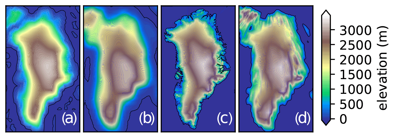
Figure 1The climate model topography for the PD (a) is from the ERA-Interim data set, and that for the LGM (b) is from the CCSM4 simulation. The model topography used for the PD is ETOPO (c), and ICE-6G is used for the LGM (d). For the plot all topography below 5 m was considered sea level for the climate models.
Global sensitivity analysis (GSA) is a variance-based method that allows for an assessment of the model sensitivity over the entire parameter space. In contrast to other sensitivity methods, it assesses the full parameter space simultaneously. The method has been applied previously to snowpack (Sauter and Obleitner, 2015) and recently to alpine glacier modeling (Zolles et al., 2019). The method is based on algorithms developed by Saltelli et al. (2000, 2006, 2010), utilizing the setup of the ensemble hypercube (Sobol et al., 2007). To compute both sensitivity indices, the estimator from Sobol et al. (2007) was used. The probabilistic framework provides an estimate of the sensitivity of the model output to the individual input variables, including parameters and data. The GSA is independent of model calibration and tuning. The model output Y is a function of the input parameters Xi: ). There are two normalized values that quantify the model sensitivity for each input parameter Xi: the first- or main-order sensitivity index SXi and the total sensitivity index STi of parameter Xi. The first order index denotes the sensitivity of the model towards the parameter Xi only, while the latter includes all the interactions of Xi:
where E is the expectation value of a given observable such as the SMB. VY is the total variance of the given variable, and VXi the variance that only depends on the input parameter Xi. X−i denotes the whole parameter space excluding any variation in Xi. The first-order index calculates the mean model output () for each representation of Xi and then assesses the sensitivity by calculating the variance for all values of Xi.
The total index can be compared to the local sensitivity index that is often determined around the optimal model setting, but the GSA presented here does not rely on a predetermined optimal parameter setting. VXi(Y) varies the parameter Xi along its dimension but is computed for all possible points of the parameter space instead of for the optimal one. For the detailed algorithm refer to Saltelli et al. (2010). As under-sampling is assumed because of the relatively low numbers of simulations, bootstrapping is applied to the ensemble and multiple sensitivity values are reported. Both indices are normalized with the variance of the whole ensemble VY. We are limiting the detailed discussion to the total index STi, as BESSI is a highly correlated model.
Cuffey and Paterson (2010)Cuffey and Paterson (2010)Cuffey and Paterson (2010)Braithwaite (2009)Greuell (1992)Aoki et al. (2003); Born et al. (2019)Bougamont et al. (2005)Oerlemans and Knapp (1998)Greuell (1992); Born et al. (2019)Table 1The parameter ranges for the free model parameters are broad and based on previously published values (Born et al., 2019). The firn albedo may not exceed the fresh snow albedo, and its value was limited to 0.65 during the LGM. All parameters are distributed following a pseudo-random Sobol sequence.
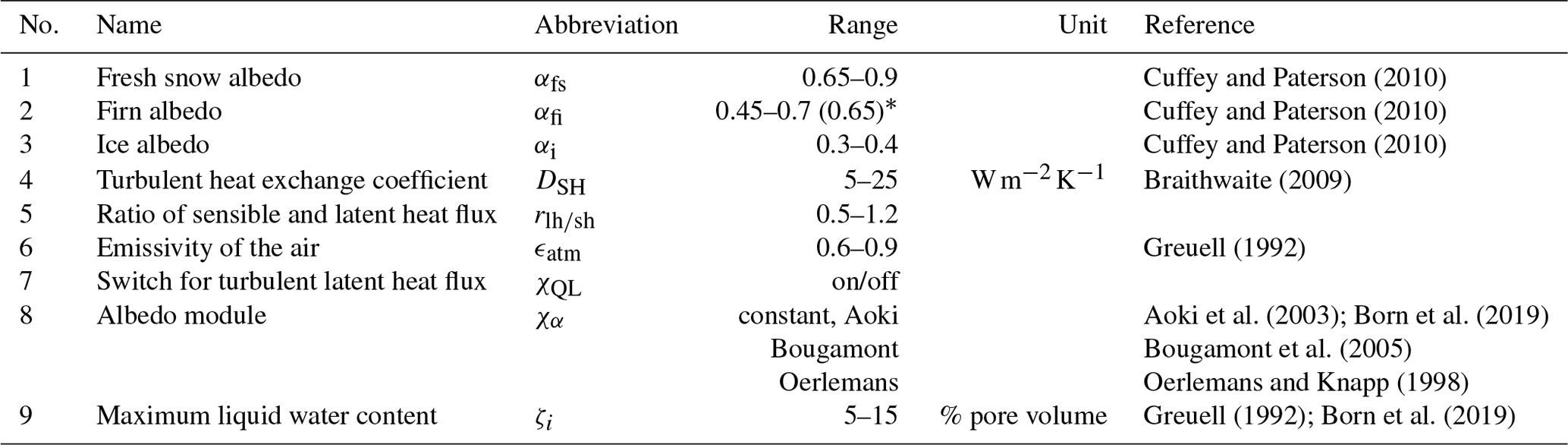
* The firn albedo may not exceed the fresh snow albedo.
We are using nine free model parameters (Table 1). The initial ensemble was generated using a Sobol sequence which consisted of 2000×9 members for the PD and 1000×9 members for the LGM. This sequence spans a 9-dimensional unit hypercube. For computing both sensitivity indices the estimator from Sobol et al. (2007) was used. It splits the initial sequence into two subsets, A and B, each consisting of one-half of the initial sequence (1000×9 or 500×9). Then an additional set of matrices , which are based on the matrix B where the values for parameter Xi are replaced with those from subset A, are created. The matrices A, B, and are then used to estimate the model sensitivity. A detailed description of the algorithm can be found in Sobol et al. (2007) and Saltelli et al. (2010). The whole ensemble consists of members, with N being the base sample (1000 in the case of the PD) and k the number of parameters (nine; Table 1).
The full ensemble for the present-day climate has 11 000 members; that for the LGM climate has 5500. The initial hypercube with a length of [0,1] in each dimension is linearly transformed to the intervals given in Table 1, with the exception of the latent heat flux switch and the albedo module. These two parameters have two and four discrete values, respectively, and the parameter space is split equally between them. The model simulations are carried out with the generated parameter matrix. We are using bootstrapping to estimate the sensitivity indices. For each bootstrap Eqs. (17) and (18) are evaluated. Finally, we report the mean sensitivity indices and their standard deviation. The results were checked for consistency (, SXi≤STi). The ensemble size used during the LGM is at the absolute lower limit of applicability for GSA, as the standard deviation of the sensitivity indices is large (Fig. A1). The GSA works well for the SMB, latent heat flux, and melt, sometimes with increased uncertainty, but fails for the 10 m firn temperature for example. Due to the larger ensemble, the confidence in the PD ensemble is higher but not by a large enough margin to justify the additional computation time relative to the 5500 members of the LGM ensemble. BESSI is a complex model with all parameters interacting, and SXi provides less information. Therefore, the results mainly focus on the total sensitivity index STi.
The GSA was computed for five different outputs: albedo, vapor flux, snowmelt, surface mass balance, and surface temperature, which are based on average yearly sums for SMB, melt, and vapor flux or temporal averages for albedo and temperature over 100 years. Surface temperature results are uncertain, and only tendencies can be extracted as the surface temperature is largely influenced by the annual cycle and fresh snowfall on an ice surface.
3.1 Global sensitivity analysis – GSA
GSA in the present day (PD) over elevation bands. The main focus of the results is on the surface mass balance, and discussion is limited to the total sensitivity index (STi), due to limited information that can be extracted from SXi in complex models. The sensitivity of the SMB for different elevation classes for the present-day ice sheet is shown in Fig. 2. In the region from 0–1000 m the largest sensitivity is associated with the parameter uncertainty in the atmospheric emissivity ϵatm with a normalized total sensitivity index of about 0.8. The second-most-influential parameter is the turbulent heat exchange coefficient DSH, followed by the snow albedo (Fig. 2a). The general features are similar up to 2000 m (Fig. 2b), with a slight decrease in the sensitivity to DSH. In regions above 2000 m (Fig. 2c, d, e) the SMB is sensitive to a much wider range of parameters: the atmospheric emissivity, the fresh snow αfs and firn albedo αfi, the choice of albedo module χα, the turbulent heat flux coefficient DSH, and the turbulent latent heat flux switch χQL. While the importance of χQL increases with elevation, the importance of αfi decreases. The sensitivity of the fresh snow albedo αfs increases up to 0.4 at 2500 m but not further. With the increasing sensitivity of multiple parameters, the relative sensitivity to ϵatm decreases, leading to χQL being almost equally important in the region with the highest average elevation. The local SMB in regions above 2000 m is impacted by multiple parameters, while the integrated mass balance is dominated by the atmospheric emissivity, with the snow albedo and turbulent fluxes having a minor influence.
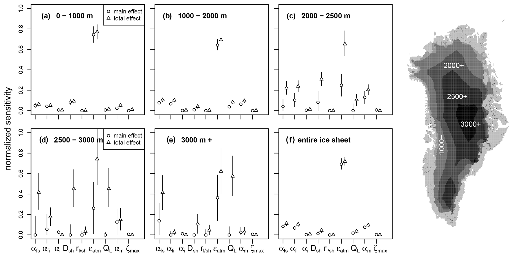
Figure 2The global sensitivity analysis of the PD SMB provides the main-order effect (circle) and the total effect (triangle). The main-order effect shows the model sensitivity to the parameter alone, and the total includes its interaction with other parameters (Sect. 2.3). The two indices are displayed for all nine parameters over the different elevation bands ranging from 0–1000, 1000–2000, 2000–2500, and 2500–3000 to above 3000 m and for the entire ice sheet. The symbol represents the mean value of the sensitivity index with the bars as ±1σ. The elevation bands of the present-day topography over Greenland are displayed on the right; the analysis is only performed for cells where ice is present. A similar figure for the LGM is found in the Appendix (Fig. A1).
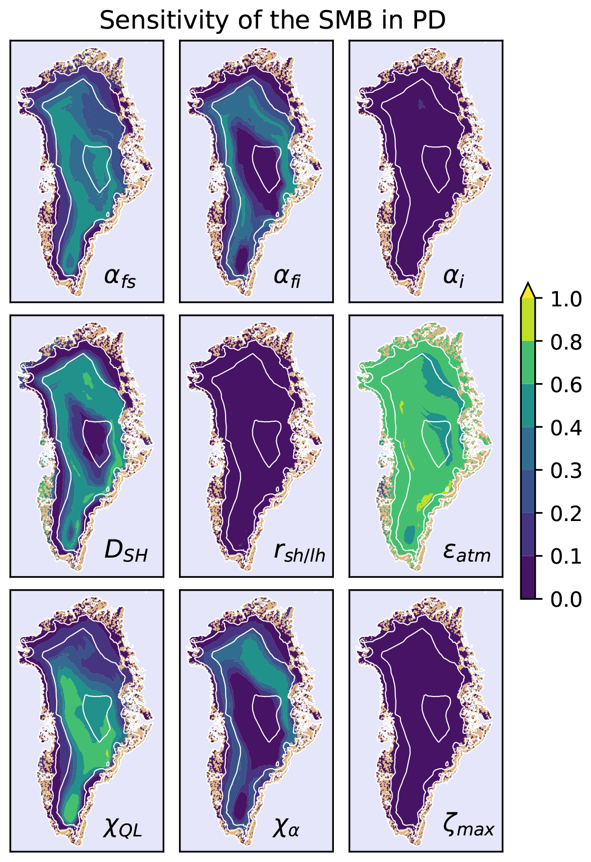
Figure 3Global sensitivity in the PD. The total sensitivity index of the SMB of every parameter for the PD is displayed for every ice-covered grid cell. The ice-free land is in brown; the ocean is in light blue; 1000 m contours are in white. The sensitivity is largest for the atmospheric emissivity ϵatm, followed by the fresh snow and firn albedo , the turbulent heat exchange coefficient DSH, and the latent heat flux switch χQL. The SMB is not sensitive to the ice albedo αi, the ratio of the turbulent exchange coefficients , and the liquid water content ζi. The maps do not include uncertainty, but the uncertainties in the sensitivities are of the same order of magnitude as shown in Fig. 2.
Spatial pattern of GSA in the PD. The global sensitivity maps for all parameters are displayed in Fig. 3. The GSA was calculated for each grid cell individually. The general trends are similar to the elevation averages, but the spatial pattern shows important additional details (Fig. 2). The SMB is sensitive to ϵatm over the entire ice sheet. The SMB is also sensitive to χQL in the interior of Greenland, and χQL can be considered a sensitive parameter for most of the ice sheet apart from the regions of very high melt. In the interior of very high elevation, the most sensitive of the three snow-albedo-related parameters is the one for fresh snow αfs, while at elevations below 2000 m, the firn snow albedo αfi and the chosen type of albedo parameterization χα is more important, the latter in particular in the northeast, where fresh snowfall is infrequent. The SMB is sensitive to DSH at the ice caps in the west and on the ice sheet above 1500 m; only at the top of the ice sheet is its influence reduced. The ice albedo αi plays a minor role in the north but is generally of very low impact. Additionally, ζmax as well as is of minor importance.
The dominance of ϵatm is a result of the change in total heat flux associated with its parameter uncertainty. At an annual average air temperature of −10 ∘C, a change in the atmospheric emissivity from 0.6 to 0.9 increases the heat flux by 80 W m−2, while a change in albedo from 0.9 to 0.6 only increases the energy input by 40 W m−2 for typical values of solar radiation annual averages. Similarly, the sensible heat flux is smaller than the other heat fluxes over most of the ice sheet (monthly averages from −20 to +50 W m−2 with ), so even a doubling will not be larger than the change in atmospheric emissivity on an annual basis. The relatively low impact of the ice albedo αi is due to the small exposure time and the small parameter range. An ice albedo change of 0.3 to 0.4 will at most result in an annual average energy change of 10–20 W m−2, but the ice is never exposed for the whole year. Rather the date of ice exposure, which is a result of the energy fluxes prior to its exposure and associated with an surface albedo change from 0.55–0.9 to 0.3–0.4, is much more important. The SMB in regions above 1000 m is sensitive to the snow albedo, which in turn is a function of snowfall, snow temperature, and the chosen albedo parameterization. Each albedo model treats these processes differently. While the basic one only distinguishes between dry and wet snow, the others account for snow aging ranging from time over time–temperature to time–temperature–wetness dependency. The choice of albedo model is not important in the interior of Greenland, as temperatures are low, albedo decay is slow, and the snow does not get wet. At slightly lower elevations there is an interplay of the fresh snow albedo αfs and firn albedo αfi and the chosen decay parameterization χα, with a larger impact of the fresh snow albedo, as snowfall is not frequent and decay rates at around −10 ∘C are of the order of a few weeks (Sect. 2.1.1). An exception is found in the northeast, which is characterized by the driest climate on Greenland. The less frequent precipitation and therefore albedo resetting explains a larger dependency on the decay rate and the choice of albedo module. The northeast of Greenland is furthermore an area higher up on the Greenland ice sheet where χQL is less important. Due to the low amount of precipitation, the SMB is quite sensitive to changes in the surface energy balance (SEB). Ensemble members with very high energy balance (low albedo, high emissivity) lead to a melting state, which results in very large changes in SMB relative to the small changes associated with condensation and sublimation. The large impact of DSH at the western coast is due to the large air–surface temperature difference, while in the interior of Greenland the atmospheric temperature is much closer to the snow surface temperature.
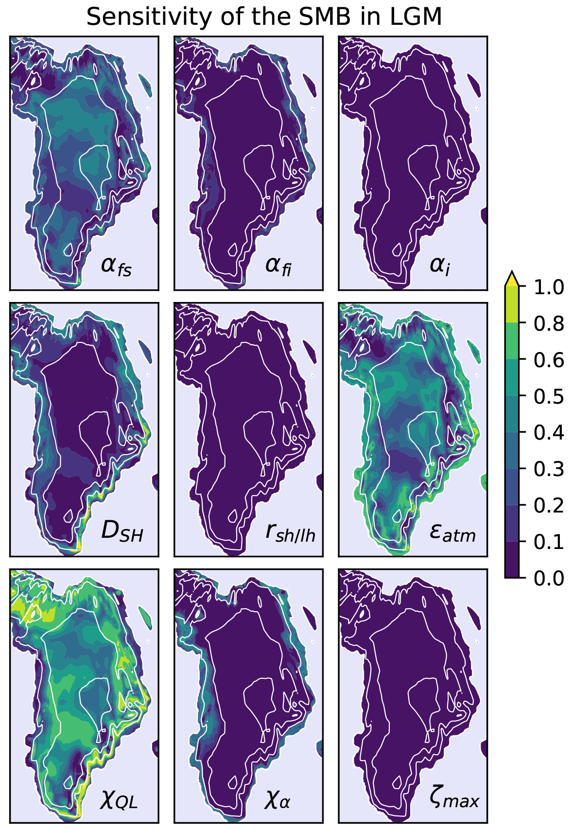
Figure 4Global Sensitivity in the LGM. The total sensitivity index of the SMB of every parameter for the PD is displayed for every ice-covered grid cell. The ice-free land is in brown; the ocean is in light blue; 1000 m contours are in white. The total sensitivity index of the surface mass balance for the LGM is more variable than during the PD. The model shows the greatest sensitivity towards χQ and the atmospheric emissivity ϵatm followed by the fresh snow albedo αfs. Firn albedo αfi and the albedo module χα as well as the turbulent exchange coefficient DSH are important around the margin. The SMB during the LGM shows almost no sensitivity towards the other parameters.
Spatial pattern of GSA at Last Glacial Maximum (LGM). The sensitivity of the SMB in the LGM shows similar features as in the PD but is shifted to lower elevations (Fig. 4). During the much colder and dryer LGM the lowest region shows an increased importance of the choice of the snow albedo module. The turbulent latent heat flux switch χQL is already as important as the atmospheric emissivity ϵatm above 1000 m, and the fresh snow albedo αfs is almost as important above 2000 m. The ice-sheet-integrated SMB shows strong sensitivity to atmospheric emissivity (–0.7), the turbulent heat flux coefficient (up to 0.8, coastal), the latent heat flux switch ( mostly > 0.4), and the snow albedo () (Fig. 4) during the LGM. The liquid water content ζmax, the ice albedo αi, and the ratio of latent and sensible heat exchange coefficient only marginally impact the SMB in either of the two climate states (Figs. 3 and 4). On the local scale χQL followed by ϵatm and αfs is the main sensitivity component in the LGM (Fig. 4). The sensible heat flux exchange coefficient DSH is important along the margin with the largest impact in the southeast. The firn albedo and the albedo module are sensitive parameters along the margin, apart from the precipitation-heavy south and southeast, where frequent snowfall resets the albedo.
The increased importance of χQL is a result of a much colder and dryer climate. The SMB is positive over most of Greenland during the LGM, even for parameter combinations leading to a high energy input. In the absence of melt, the only change to the SMB is due to sublimation and hoar formation. The dry climate also favors higher sublimation than in the PD. The vapor flux (sublimation) is mainly a net heat loss for the surface in the LGM. The surface temperature via the Clausius–Clapeyron relation has an exponential impact on the turbulent latent heat flux, resulting in a greater model sensitivity towards the atmospheric emissivity than the actual exchange coefficient DSH (Eq. 13). The incoming longwave radiation is also the largest energy source for the surface. The large impact of DSH in the southeast is due to the large temperature difference between the surface and the air. The southeast is dominated by intense precipitation and rather warm air masses even during the LGM. There is a precipitation gradient from the western coast to central Greenland: the least precipitation is found in the west of Greenland and the south of Ellesmere Island due to circulation changes due to the presence of the Laurentide ice sheet over North America in the LGM (not shown). Therefore, the albedo module is more important on the western than on the eastern margin as frequent precipitation, which is mainly snowfall during the LGM, increases the albedo more frequently. The lower model sensitivity in the LGM towards ϵatm is mainly a result of the lower air temperature with annual averages being around 10 K lower, resulting in less incoming longwave radiation and a lower absolute impact of the emissivity.
Sensitivity of other output variables in addition to SMB. We also studied the sensitivity of other model variables, namely the surface albedo, turbulent latent heat flux, snowmelt, and surface temperature. The corresponding figures (which are similar to Figs. 3 and 4) are included in the “Additional information”. The global sensitivity for the annual average albedo during the PD period is mainly influenced by the fresh snow albedo parameter, with only minor importance of the firn albedo, ice albedo, the choice of the albedo module, and the atmospheric emissivity at the ice sheet margin. As a result, the snow albedo should not be tuned with BESSI without incorporating the atmospheric emissivity in addition to the direct albedo-related parameters (Fig. GSA_albedo_ERAi/LGM in the “Additional information”).
Besides the switch (χQL) which disables the turbulent latent heat flux QL completely, the turbulent latent heat flux is most sensitive to the atmospheric emissivity ϵatm followed by the turbulent heat flux exchange coefficient DSH, mainly around the margins (Fig. A3). Around the margin the ratio of turbulent sensible and latent exchange coefficients plays a minor role (Sti≈0.1). The turbulent latent heat flux is also sensitive to the snow-albedo-related parameters () in the north. The turbulent latent heat flux QL is sensitive to neither the maximum liquid water content ζmax globally nor the ice albedo and in the interior of the ice sheet. As the effect of on the turbulent latent heat flux as well as on the SMB is low, using similar exchange coefficients for moment, temperature, and water vapor is justified within this framework. In the LGM, QL shows an increased sensitivity to αfs, while the DSH is less important around the margin, due to lower atmospheric temperatures and slower albedo decay (not shown). The albedo module and the firn albedo play almost no role in either case.
The average snow temperature is mainly influenced by ϵatm, αfs, DSH, and χQL, though uncertainties in the sensitivity are rather large due to temperature resetting in the event of snowfall on ice or shallow snowpacks.
Snowmelt is closely linked to the SMB and shows similar sensitivities to those reported for the SMB. Just as expected, the impact of the latent heat flux switch is lower as it is mainly important in regions with an absence of melt (Fig. 3).
3.2 Ensemble statistics
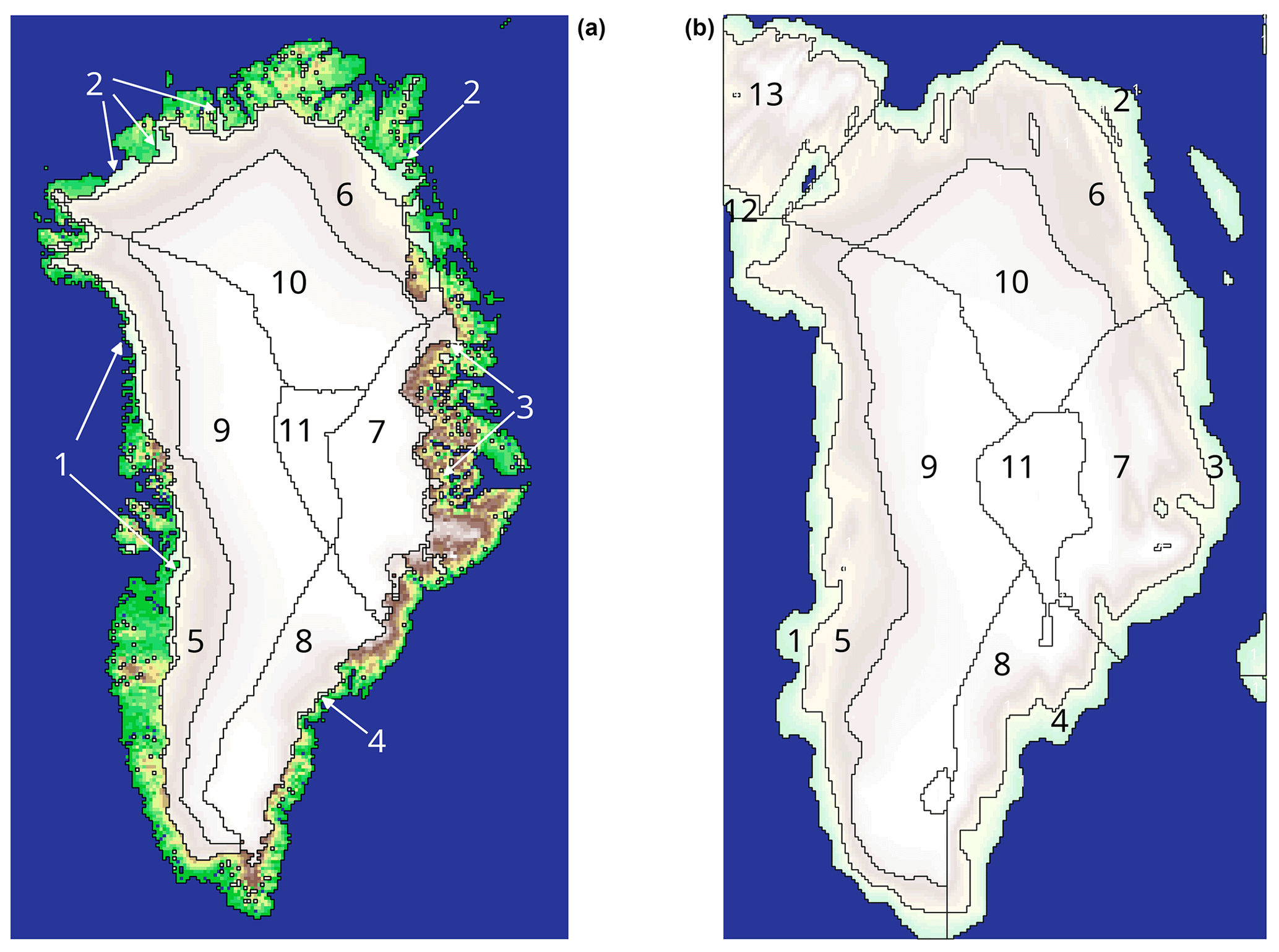
Figure 5Greenland is split into 11 regions based on elevation, geographic, and climatic similarity for the PD (a) and the LGM (b). There are four different sections with SW–W, N, E, SE, and the area around Ellesmere island for the LGM. Each section is split into three elevation bands ranging from 0–1000–2000–3000 m. During the present day there are three regions in the west and north from 0–1000–2000–3000 m (1, 5, and 9; 2, 6, and 10). The southeast and east regions are precipitation driven, and the change in SMB with altitude is less developed; therefore 1000–3000 m is joined to one region (4, 8; 3, 7). There is one additional region in the center which is at elevations above 3000 m (11). Ice-covered areas are in white with slight elevation shading in the background. The ice-free area is based on elevation coloring with green as the lowest and brownish the highest.
PD regional parameter dependencies. The GSA highlights the surface mass balance as the variable most sensitive to atmospheric emissivity and the latent heat flux switch irrespective of background climate. The GSA method has the drawback that it gives no information about the sign and absolute magnitude of the SMB changes. Physical processes and associated parameters, which result in either surface heating or cooling, will be analyzed based on ensemble statistics explained in the following. On the other hand, an increase in albedo and a decrease in atmospheric emissivity always lead to an increase in surface mass balance. The ensemble statistics also give additional information about parameter sensitivities which were well analyzed with GSA. We split Greenland into 11 different regions for the PD and 13 for the LGM (2 more around Ellesmere Island) based on elevation, ice divides, geography, and climatological similarity for this analysis. In particular most of the west coast shows similar behavior and is therefore only a single region (Fig. 5). This is a regional spread of the elevation bands used in Fig. 2. For each region the parameter range is split into 20 equally spaced intervals for which the 5 %, 25 %, 33 %, 50 %, 66 %, 75 %, and 95 % quantiles are calculated. The binning is necessary as the ensemble was not created with parameters at regularly spaced intervals. The most interesting features are seen for the parameters where the effect changes sign depending on the atmospheric conditions, like for the turbulent heat exchange coefficient. We discuss the selected region 5 and the turbulent latent heat flux in depth here, while the complete set of figures is included for reference in the “Additional information”.
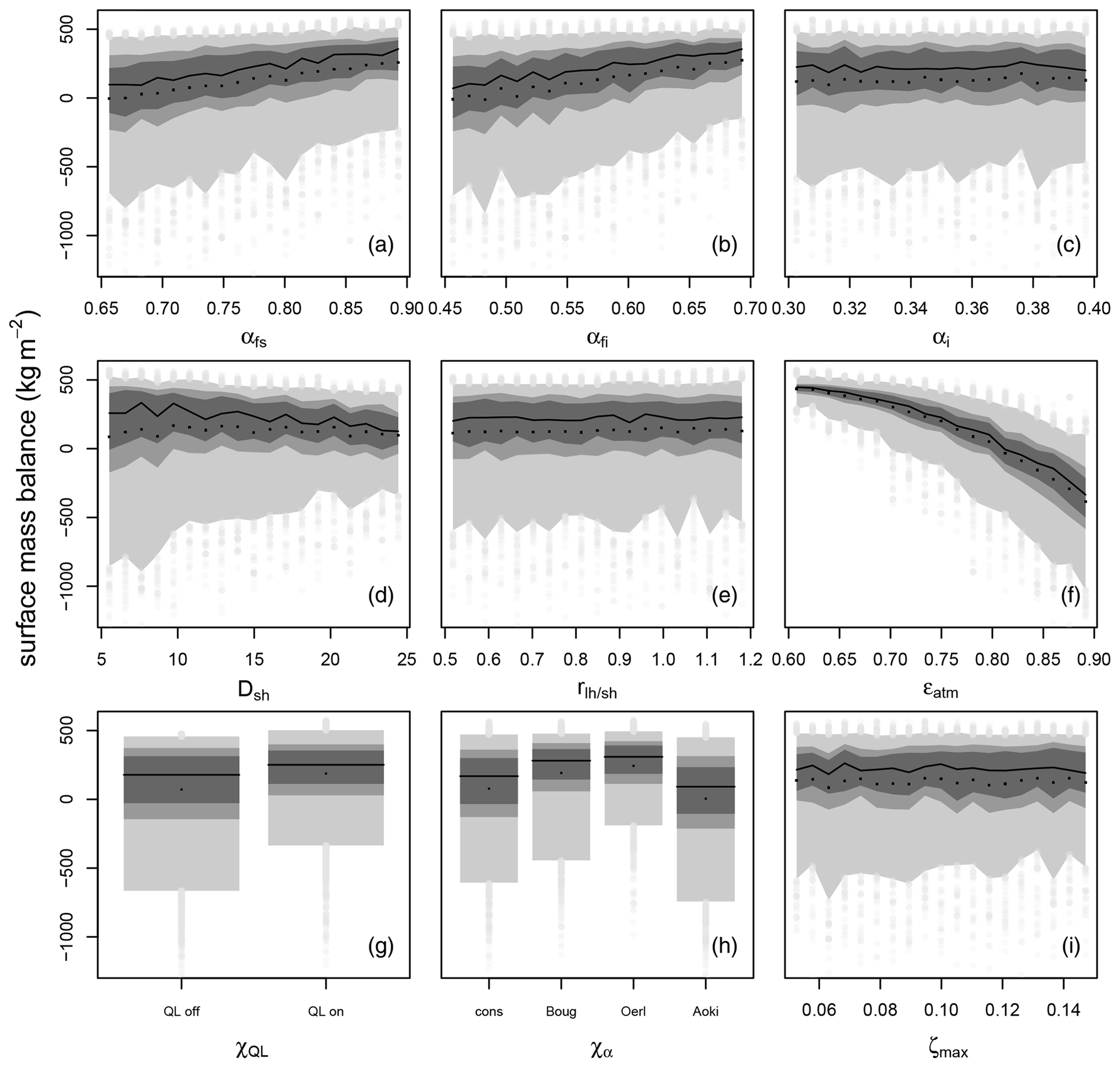
Figure 6The ensemble statistics for the surface mass balance for region 5 (west 1000–2000 m) in the PD. The 5th and 95th, 25th and 75th, 33rd and 66th, and 50th quantiles are displayed in progressively darker shading. Black points represent the ensemble mean, and the grey points correspond to the rest of the ensemble, apart from outliers (max five per bin allowed), which are removed to improve readability. Each plot represents the range of one parameter with αfs, αfi, and αi in the top row; DSH, , and ϵatm in the middle; and , χα, and ζmax at the bottom. As and χα have two and four discrete values, respectively, the parameter range is not split into 20 intervals.
In Fig. 6 the impact of the various parameters on the PD SMB is shown for region 5, the western region of Greenland ranging from 1000–2000 m where the equilibrium line for the present-day ice sheet is located. The dominant parameter is the atmospheric emissivity ϵatm. Over the range of plausible values, ϵatm reduces the median of the SMB by almost 800 kg m−2. The atmospheric emissivity and the SMB are inversely correlated, and the relationship is non-linear with greater effect at larger values. The spread of the ensemble, i.e., the variance of the SMB as a result of other parameters, increases too. The increase in the SMB with the snow-albedo-related parameters αfi and αfs is smaller and the width of the distribution decreases (panel a, b), as even very low albedo parameter values do not necessarily lead to a negative SMB in the western region. An increase in DSH slightly reduces the median SMB, but the spread decreases. Ice albedo αi, liquid water content ζmax, and have almost no impact. The SMB increases in the presence of turbulent latent heat flux due to the heat loss of sublimation in region 5. With all albedo modules the ensemble has a wide spread, but the variation is smallest for the time-dependent decay (Oerlemans and Knapp, 1998) which also has the highest median mass balance, as it neither has an instant albedo drop upon reaching the melting point (constant) nor accounts for the liquid water mass in the snowpack. The parameterization based on temperature, wetness, and time has the lowest median SMB.
The strong impact of the emissivity on the surface energy balance and therefore also on SMB is due to the larger annual average of the incoming longwave radiation relative to the shortwave, precipitation, and turbulent fluxes. In the PD climate, the largest energy source for the snow is incoming longwave radiation. As atmospheric emissivity ϵatm decreases, less energy is available for melt in region 5. In the absence of melt, surface mass balance response is only due to the sublimation, and since the vapor flux has a modest absolute impact on the SMB, the spread of the ensemble is low. Vice versa, at large ϵatm values, warming, as well as potentially early melting of the snowpack, occurs in many grid cells, leading to a positive feedback effect with lower albedo. In agreement with the GSA (Fig. 3) the firn albedo αfi is almost as important as fresh snow albedo αfs. The equilibrium line altitude (ELA) is located in region 5, and snow temperatures are rather warm, resulting in a large impact of snow albedo decay and its parameterization. The constant albedo parameterization spreads more than 1000 kg m−2, as the albedo is very sensitive around the ELA, changing instantly from αfs to αfi when the snowpack reaches the melting point, while the albedo parameterizations based on Oerlemans and Knapp (1998) and Bougamont et al. (2005) have a temporal decay relative to the instant one in the constant case. Bougamont et al. (2005) have a snow-temperature-dependent increased decay rate, which is even more pronounced in the wet case, leading to an ensemble that is less skewed than those of the constant case and Aoki et al. (2003). The last albedo parameterization decays faster than the other two at warmer temperatures, leading to lower albedo than for all other albedo parameterizations before the melting point is reached. Additionally, there is a difference between the models in the case of snowfall.

Figure 7The ensemble statistics for the surface mass balance of the QLon sub-ensemble for region 5 (west 1000–2000 m) in the LGM. The 5th and 95th, 25th and 75th, 33rd and 66th, and 50th quantiles are shown in progressively darker shading. Black points represent the ensemble mean, and the grey points correspond to the rest of the ensemble, apart from outliers (max five per bin allowed), which are removed to improve readability. Each plot represents the range of one parameter with αfs, αfi, and αi in the top row; DSH, , and ϵatm in the middle; and , χα, and ζmax at the bottom. As and χα have two and four discrete values, respectively, the parameter range is not split into 20 intervals. Figure A2 shows a similar plot for the entire LGM ensemble.
Differences in the LGM regional parameter dependencies. During the LGM the western region between 1000–2000 m (not corresponding to the identical geographical area in the PD due to topographic differences) shows positive but low SMB with a lower spread of the ensemble (Figs. 7, A2). The climate in the west of Greenland in the LGM is characterized by a much lower air temperature, slightly more annual mean radiation, and lower precipitation. There are three distinct differences to in the PD:
-
The lower air temperature reduces the impact of ϵatm and produces a more positive SEB.
-
The impact of αfi and χα is drastically reduced. The importance of αfs increases relatively to ϵatm (Fig. 7). The incremental increase in snow albedo with snowfall gives slightly lower albedo in the dry climate. The colder snowpack due to a more positive SEB has a slower snow albedo decay (for the albedo subroutines which parameterize the decay), no melting, and almost no impact of associated parameters.
-
Enabling the latent heat flux results in a decrease in SMB, as sublimation prevails in the LGM over the entire year. However, in the absence of melt the increase in sublimation results in a mass loss, rather than the reduced melt via cooling due to sublimation during the PD conditions. Furthermore, the non-linearity in the SMB in the LGM almost vanishes for ϵatm and αfs as there is hardly any melt and associated snow–ice albedo feedback.
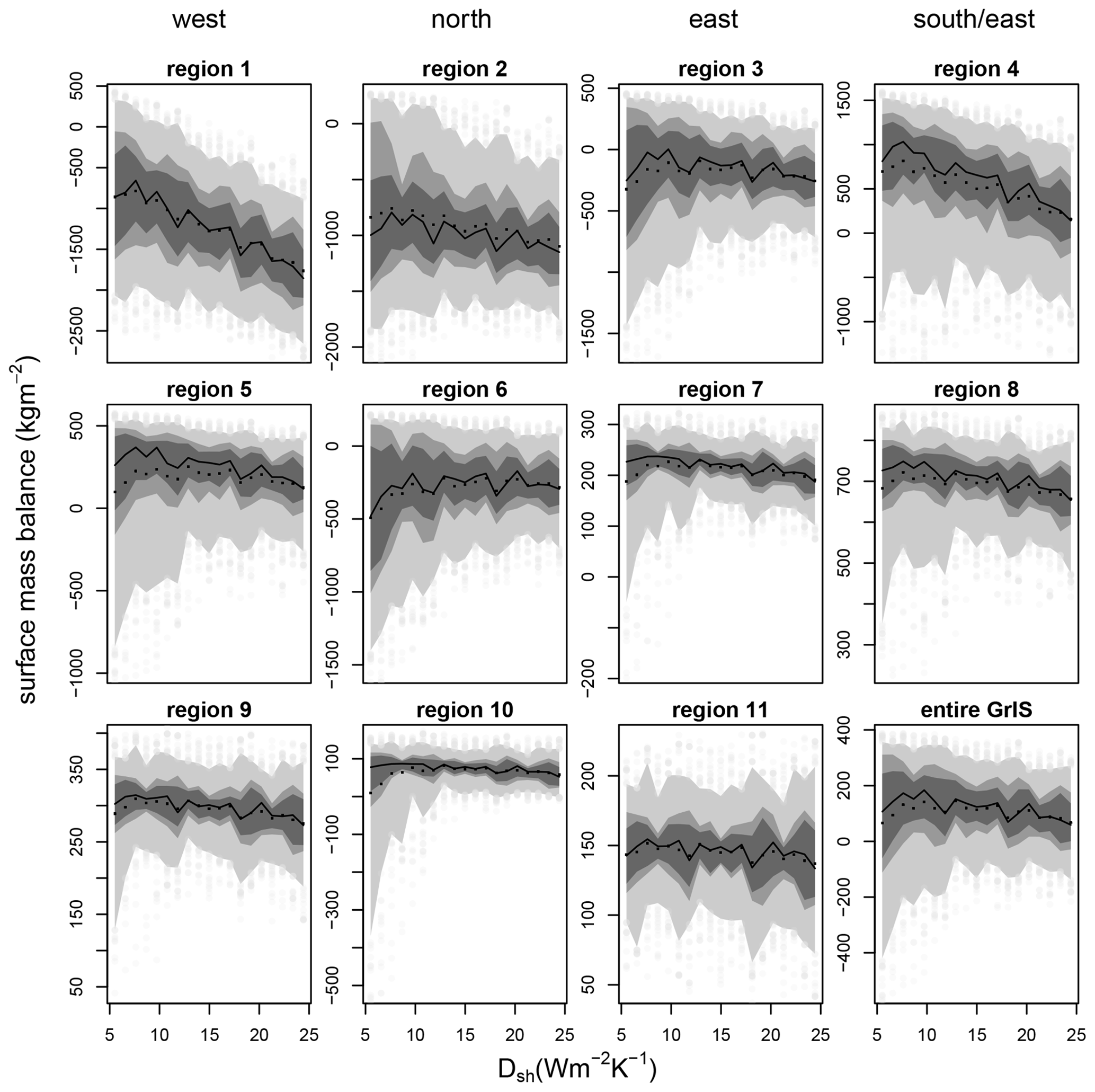
Figure 8The dependency of the SMB on the turbulent heat exchange coefficient DSH is displayed in a similar manner to in Fig. 7 for the PD. The shading represents the different quantiles: 5th and 95th (light grey), 25th and 75th (grey), 33rd and 66th (dark), and the median (solid black line). The black dots are the ensemble mean based on 20 intervals. The panels are sorted by elevation and regions, with the lowest elevation (0–1000 m) in the top row and the highest elevation at the bottom. Each column is related to a region in Greenland: W, N, E, SE–S (Fig. 5).
Impact of the turbulent heat flux exchange coefficient on the SMB as an example for the PD. The SMB dependency on the turbulent heat flux coefficient DSH varies over the different regions (Fig. 8). The turbulent sensible heat flux may be either a heat loss or a heat gain for the surface depending on the difference between atmospheric and surface temperature, which is why we present a deeper look into the related parameter (the figures for all other parameters are available in the “Additional information”). Only the sub-ensemble with an active turbulent latent heat flux (χQL−on) is shown in Fig. 8 because in regions without melt, 50 % of the simulations (χQL−off sub-ensemble) will show a similar SMB. The overall width of the SMB distribution decreases with altitude. The lowermost regions in the west and southeast (1, 4) show a trend to more negative mass balances with larger exchange coefficients. Regions 3, 5, 6, 10, and to a lesser extent 2 and 7 show a distinct decrease in the width of the SMB distribution of the ensemble with increasing DSH and a slight decrease in the mean (excluding region 6). The general negative trend for the SMB with DSH is a result of higher air than snow surface temperatures. The negative trend is most pronounced at the lower regions of the west and south, where warm air advection is frequent, resulting in increased melt due to the heat supplied by the sensible heat flux. The regions are also quite moist, in particular in the southeast (region 4), leading to a positive turbulent latent heat flux (condensation), which in turn heats the surface too.
The northeast (region 2, 3, 6, 7) of Greenland is colder and drier, resulting in decreased turbulent fluxes, and therefore the effect of DSH on the SMB and surface energy balance is lower. The ensemble spread is narrower at higher altitudes (7–11) due to a generally positive mass balance. An increased energy input due to any parameter will raise the snow temperature, but in the absence of melt the mass balance does not change strongly. Still, the snow temperature change alters sublimation, accounting for the remaining variability in SMB. This is pronounced in region 10: at low exchange coefficients melt is still possible if other parameters result in a strong positive energy input, leading to skewness towards negative SMB. At a large exchange coefficient the tight coupling with the heat reservoir of the atmosphere limits melt and the skewness towards negative SMBs vanishes, while the median stays almost constant. The SMB does not strongly vary with parameter DSH in region 10; rather the parameter acts as a buffer of the SMB. With strong turbulent sensible heat exchange the surface temperature will be buffered by the air temperature heat reservoir, so the spread of the ensemble becomes narrow. The buffering effect is visible for most regions, where air temperatures are below the melting point for most of the year (2, 3, 5, 7–10).
The turbulent heat exchange coefficient DSH also impacts the SMB via the turbulent latent heat flux (QL in Eq. (12), additional figure available in the “Additional information”). QL becomes more negative with an increasing exchange coefficient. Firstly, the higher surface water vapor pressure of the warmer snow/ice surface, as a result of the heating by the turbulent sensible heat flux QSH, increases sublimation. Secondly, the absolute vapor flux is also larger with a higher exchange coefficient. The annual average of the ensemble over Greenland is a negative turbulent latent heat flux, meaning sublimation occurs more often than condensation. At larger exchange rates more mass can be moved, and therefore the variation over the ensemble increases.
The average SMB increases at low elevations if the turbulent latent heat flux is switched on (χQL−on sub-ensemble); it decreases above 2000 m and is almost constant above 3000 m, where the annual average of the latent heat flux is almost zero. The first trend is a result of reduced melt due to a negative latent heat flux (sublimation), and the SMB increase is therefore most pronounced in the northeast. This is a region where melt only occurs for a few extreme ensemble members, so the sublimation is the only mass loss, and therefore the SMB decreases with increased sublimation.
Ensemble statistics of other parameters for the PD. The other parameter results are consistent with the GSA: an increase in ϵatm decreases the SMB, but melting increases disproportionally with higher emissivity. The high impact of ϵatm is mainly related to the all-year-around impact altering ice exposure and albedo decay. The snow albedos increase the SMB, with the fresh snow albedo being more important. The SMB ensemble plots do not show any dependency on ice albedo and liquid water content, and the mean is also unaffected by . Additional figures are available in the “Additional information”.
LGM. The general features are similar to those in the PD. Larger values of DSH reduce the variability in or impact of the other parameters, resulting in slightly lower SMB. Similarly to for the GSA, a shift to lower elevations is seen. The impact of DSH on the SMB is negligible above 2500 instead of above 3000 m for the PD and melt tails are limited to below 2000 m. ϵatm, as well as the snow-albedo-related parameters, has less influence during the colder period.
Sensitivity of the 10 m firn temperature. In addition to the SMB, the sensitivity of the 10 m firn temperature was assessed. This was not possible for the GSA due the limited sample size. We limited the analysis of the firn temperature to 13 locations in the interior of Greenland. The firn temperature at these mostly central locations is sensitive to three parameters: ϵatm, αfs, and DSH. The first two have a rather linear impact with increasing temperature with increasing emissivity and decreasing albedo. The turbulent heat exchange coefficient has a similar effect on the 10 m firn temperature to that shown for region 5. At small DSH values the 10 m temperature has a larger variability depending on the other two sensitive parameters, while at large values the air temperature buffers the snow temperature, even down to 10 m. The sensitive parameters are the main drivers of the SEB, which determines the 10 m temperature in those areas as discussed previously for the SMB. The only difference to the SMB for regions at higher elevations is the insignificance of χQL. The turbulent latent heat flux has only a minor importance for the SEB, but in the absence of melt, the vapor flux is the only SMB change. Tuning the model for the 10 m firn temperature only provides information about the sensitive parameters, which are ϵatm, αfs, and DSH.
In this study we assess the model sensitivity due to parametric uncertainties. Cloud cover and the associated atmospheric radiation are large uncertainties in both present-day and glacial climates. The uncertainty in cloud cover is represented by the large parameter uncertainty in the atmospheric emissivity ϵatm. The SMB is most sensitive to ϵatm under present-day (PD) conditions. The sensitivity of the SMB is not drastically different during the Last Glacial Maximum (LGM). However, lower atmospheric temperatures reduce the impact of the atmospheric emissivity while also leading to fewer areas where melt and runoff occur. The relative contribution of the mass flux associated with the turbulent latent heat flux to the SMB increases drastically during the LGM (4 % to 15 % of the total mass flux), making the turbulent latent heat flux switch the model's most sensitive parameter in large parts of the ice sheet. The increased importance of QL is due to the absence of melt, similarly to at the highest elevations during the PD climate. Additionally, SMB values have a smaller magnitude as precipitation is lower during the LGM and therefore the relative contribution of the vapor fluxes to the SMB is larger. For an accurate modeling of the SMB over the glacial cycle, an inclusion of the turbulent latent heat flux is necessary, which may not be as important for a warmer climate.
The sensitivity metric we applied is a relative measurement that depends on two components: the absolute strength of a particular flux and the chosen parameter uncertainty range of the parameter. The latter depends on the subjective choice. We based the parameter values on published common ranges (Table 1). The incoming longwave radiation is the largest single energy source for the surface energy balance during the PD, ranging from twice the incoming solar radiation around the margin to about one-third in the interior of Greenland in the annual average. Therefore, the impact of the atmospheric emissivity decreases from the coast inwards for multiple reasons: first, temperatures are higher around the margin leading to increased incoming thermal radiation. Second, cloud cover is higher and therefore solar radiation is reduced. Lastly, at negative SMB the rate of melting depends greatly on the total energy flux and albedo decays faster for a warmer snowpack if more longwave radiation reaches the surface during winter.
It is important to differentiate between the sensitivity of the Greenland-wide integrated mass balance and the local SMB, as well as between the impact of the individual fluxes on the absolute SMB. The Greenland-wide surface mass balance is most sensitive to the atmospheric emissivity during the PD (Fig. 2). During the LGM the SMB shows additional increased sensitivity to the fresh snow albedo, the choice of albedo parameterization, and the turbulent latent heat flux. In the LGM, lower air temperatures and an ice sheet with less melt overall increases the importance of the vapor fluxes similarly to at high elevations in the PD. It is therefore not a necessity for models to include QL in a warm climate, though it is desirable. Conversely, the turbulent latent heat flux QL cannot be ignored during a colder and dryer climate. In addition, this means that although the cloud cover uncertainty may be similar during the colder period of the LGM, the sensitivity of our model towards the emissivity uncertainty is lower. Simple surface mass balance models like enhanced temperature index models are likely to create a bias as solar insolation changes are accounted for while the impact of the cloud cover on other components of the energy balance is neglected or implicitly included in the PDD factor; even under PD conditions PDD may result in bias as the impact of clouds on the SMB is highly variable (Van Tricht et al., 2016; Hofer et al., 2017).
At the local scale such as in the interior of Greenland, even in the PD climate, the vapor flux (QL) is up to one-third of the total SMB, despite its small impact on the Greenland-wide integrated scale. In addition, in the absence of melt the sublimation and condensation are the only changes to the SMB with a fixed precipitation forcing. Neglecting sublimation and condensation will result in fundamental biases over long-term simulations of the Greenland ice sheet, in particular in its interior. This needs to be considered when tuning surface mass balance models for long timescales. Tuning for the Greenland-wide SMB will mainly constrain the most sensitive parameters, which constrain certain key regions of high mass turnover but not for the bulk surface. Furthermore, the temporal differences in the sensitivities on the local scale indicate that models of reduced complexity may fail drastically for other time periods (absence of QL for example).
The sensitivity analysis shows that the uncertainty in the longwave radiation has a larger impact on the SMB uncertainty than the uncertainty in the incoming solar radiation, but as it is not defined relative to the absolute flux, this does not necessarily tell us that the SMB is most sensitive to the longwave radiation energy component. The impact each energy flux has on the absolute SMB has to be analyzed separately. The longwave radiation dominates, followed by the solar radiation. The larger sensitivity of the χQL switch in the LGM is mainly due to χQL's increased contribution to the absolute SMB. In the absence of melt and with reduced precipitation, sublimation accounts for a larger portion of the absolute SMB.
It is beyond the scope of BESSI to resolve all the physical processes. We use a simple parameterization for the incoming longwave radiation which does not accurately represent reality. The atmospheric emissivity is constant in neither space nor time. Area-distributed values may work during the observational period, but differences in the atmospheric circulation alter these patterns over the glacial cycle. We conclude that the overall model uncertainty can effectively be improved by changing the simplified representation of the longwave radiation flux as a function of atmospheric temperature and emissivity either for a more sophisticated parameterization or to use longwave radiation as climate model input. If the model were to be tuned for the Greenland-wide SMB, it would be biased towards the melt regions around the margin and therefore the atmospheric emissivity. Where possible, parameters should be calibrated via quantities which they are sensitive to. None of our parameters are to be assumed constant in space, as albedo for example strongly depends on impurities and snow temperature, but unless the uncertainty in the incoming longwave radiation is reduced, it is justifiable to work with optimized values from the PD. The current model version does not use wind fields, although they impact the SEB via the turbulent fluxes. The strength of the turbulent exchange does not have a large impact on the SMB, and the approach to neglect wind speed variability is therefore justified in the context of more uncertain parameters. The model sensitivity towards the parameters that has been found is to be set into context with the assumed forcing (climate) uncertainty.
The surface mass and energy balance model BESSI has been improved by accounting for turbulent latent heat flux and snow aging. The sensitivity of the model to the new implementations and uncertain model parameters was assessed with a variance-based sensitivity method based on two ensembles with a total of 16 500 simulations. The warm present-day and the cold Last Glacial Maximum climate were used to study the differences in the model response under different present-day and Last Glacial Maximum boundary conditions. The sensitivity analysis reveals that the inclusion of the turbulent latent heat flux is a necessity to simulate the local SMB and the integrated SMB over the entire Greenland ice sheet. The relative importance of sublimation and condensation is larger in the dry and cold climate of the LGM as air temperature and precipitation are lower.
The uncertainty associated with cloud cover and atmospheric emissivity dominates the SMB model uncertainty. With the different circulation during the Last Glacial Maximum due to the presence of the Laurentide ice sheet, a changing energy input from the atmosphere to the surface will result in an SMB response. The sensitivity study further reveals that the uncertainty in the SMB as a result of the atmospheric radiation decreases in a colder climate.
We find that uncertainties in the ice albedo and liquid water content and differences in the turbulent fluxes are of minor importance for our and likely also similar models. In order to reduce model uncertainty most effectively, the larger energy sources of shortwave and longwave radiation need to be constrained first via the snow albedo and the atmospheric emissivity.
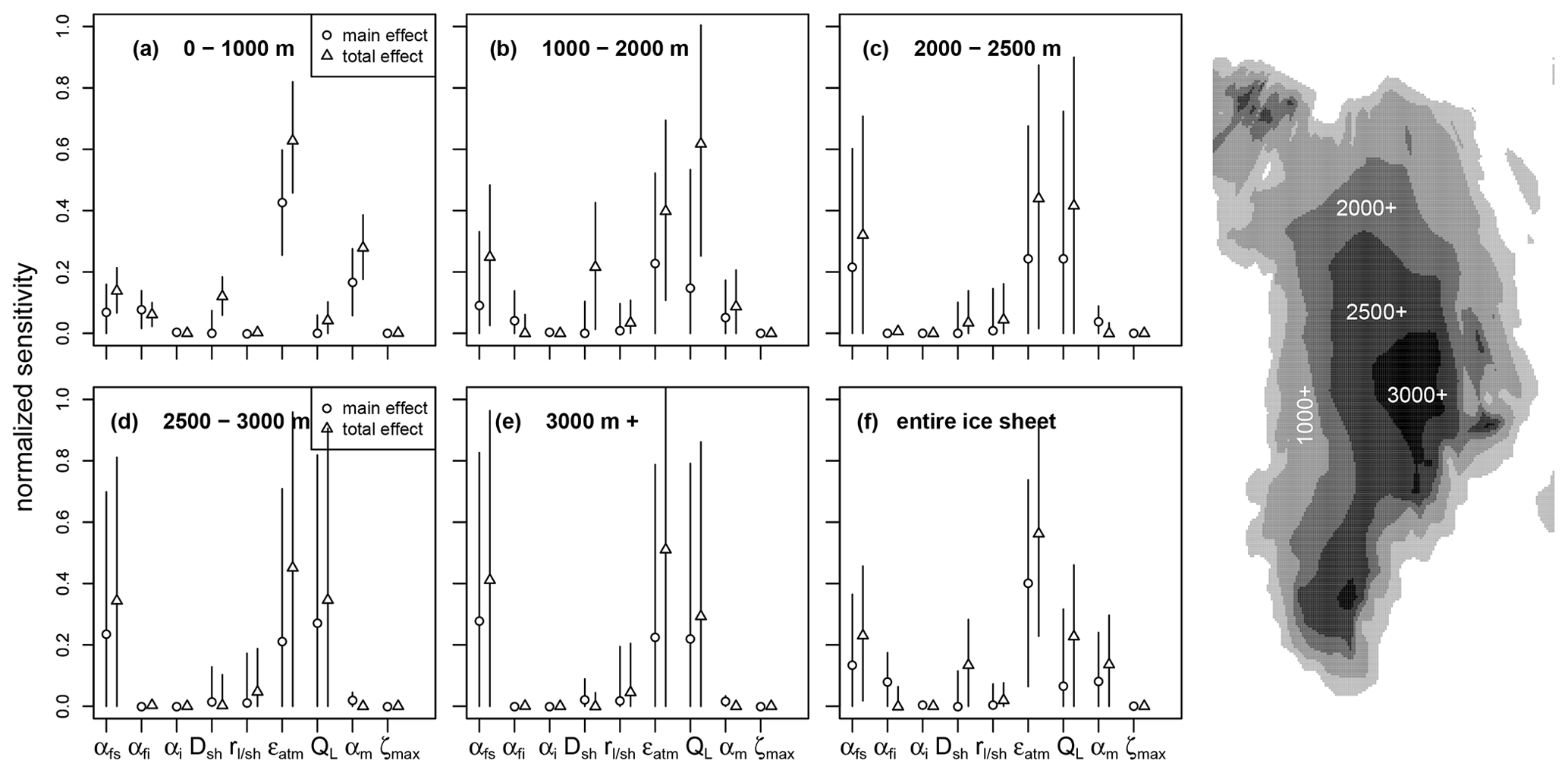
Figure A1The global sensitivity analysis of the LGM SMB provides the main-order effect (circle) and the total effect (triangle). The two indices are displayed for all nine parameters over the different elevation bands ranging from 0–1000, 1000–2000, 2000–2500, and 2500–3000 to above 3000 m and for the entire ice sheet. The symbol represents the mean value of the sensitivity index with the bars as ±1σ. The elevation bands of the LGM topography over Greenland are displayed on the right; the analysis is only performed for cells where ice is present. The uncertainty in the sensitivity indices is larger than for the PD due to the smaller ensemble size.
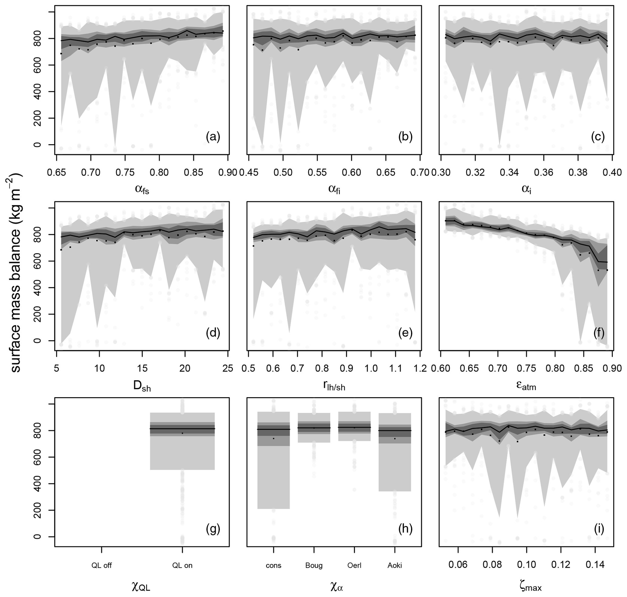
Figure A2The ensemble statistics for the surface mass balance for the entire ensemble at region 5 (west 1000–2000 m) in the LGM, showing the 5th and 95th, 25th and 75th, 33rd and 66th, and 50th quantiles in progressively darker shading. Black points represent the ensemble mean, and the grey points correspond to the rest of the ensemble, apart from outliers (max five per bin allowed), which are removed to improve readability. Each plot represents the range of one parameter with αfs, αfi, and αi in the top row; DSH, , and ϵatm in the middle; and , χα, and ζmax at the bottom. As and χα have two and four discrete values, respectively, the parameter range is not split into 20 intervals.
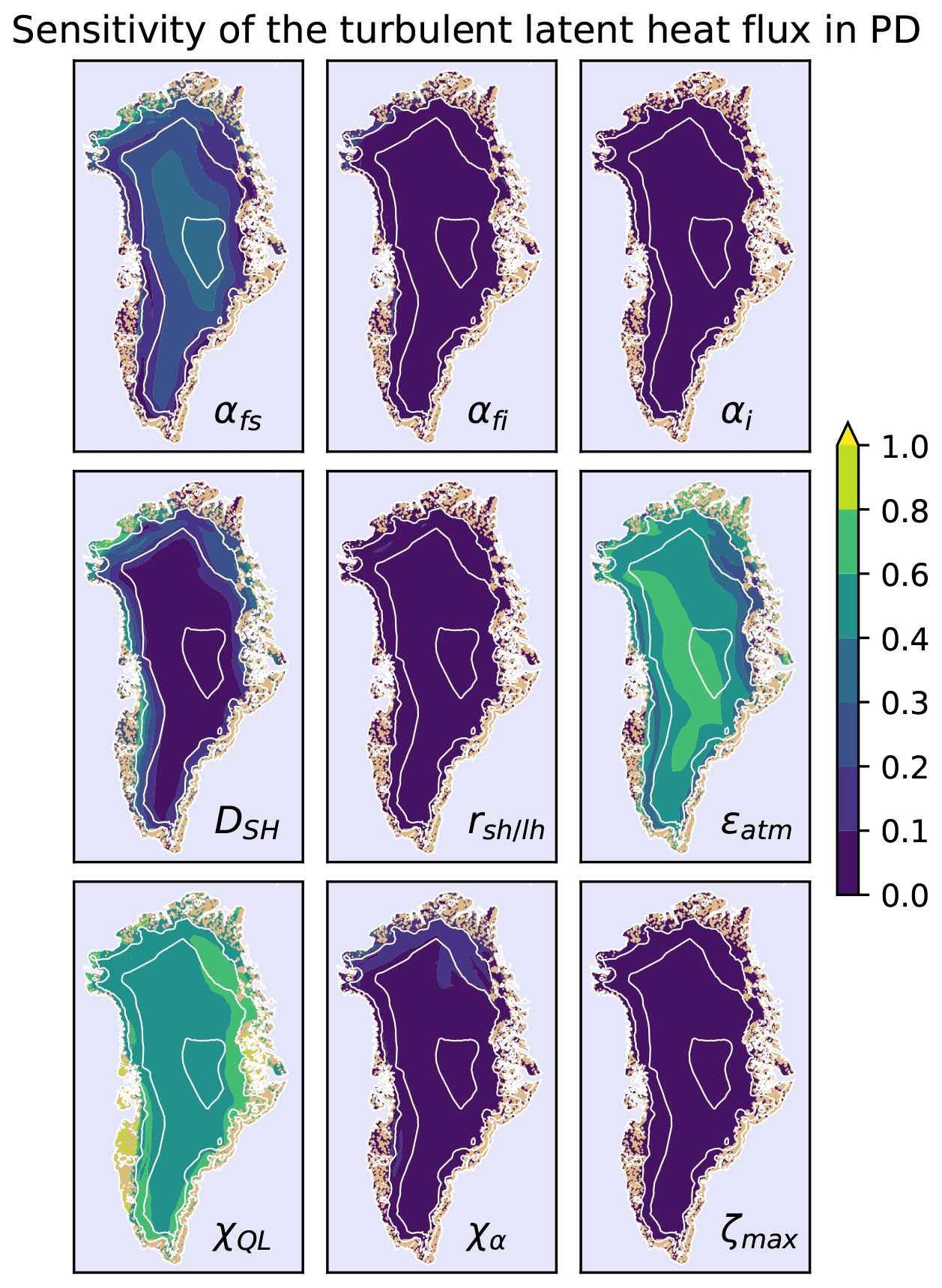
Figure A3Global sensitivity of the turbulent latent heat flux in the PD. The total sensitivity index of QL of every parameter for the PD is displayed for every ice-covered grid cell. The ice-free land is in brown; the ocean is in blue.
The BESSI model code is available on GitHub (https://github.com/TobiasZo/BESSI/tree/TobiasZo---GSA-model-version, last access: 3 June 2020). Additionally, the GitHub branch also contains the analysis and plotting scripts.
The additional information including the plots of model output variables not shown here is available at https://doi.org/10.5281/zenodo.4310369 (Zolles and Born, 2020).
TZ implemented the model changes; conducted the ensemble simulations, the sensitivity studies, and the data analysis; and wrote the main part of the manuscript. AB contributed to all aspects of this study.
The authors declare that they have no conflict of interest.
This paper was edited by Louise Sandberg Sørensen and reviewed by Andy Aschwanden and two anonymous referees.
Amante, C. and Eakins, B.: ETOPO1 1 Arc-Minute Global Relief Model: Procedures, Data Sources and Analysis [data], https://doi.org/10.7289/V5C8276M, 2009. a
Aoki, T., Hachikubo, A., and Mashiro, H.: Effects of snow physical parameters on shortwave broadband albedos, J. Geophys. Res., 108, 1–12, https://doi.org/10.1029/2003JD003506, 2003. a, b, c, d, e
Aschwanden, A., Fahnestock, M. A., Truffer, M., Brinkerhoff, D. J., Hock, R., Khroulev, C., Mottram, R., and Khan, S. A.: Contribution of the Greenland Ice Sheet to sea-level over the next millennium, Science Advances, 5, 12 pp., https://doi.org/10.1126/sciadv.aav9396, 2019. a, b
Beven, K.: Changing ideas in hydrology – The case of physically-based models, J. Hydrol., 105, 157–172, https://doi.org/10.1016/0022-1694(89)90101-7, 1989. a
Bintanja, R., Van de Wal, R., and Oerlemans, J.: Global ice volume variations through the last glacial cycle simulated by a 3-D ice-dynamical model, Quatern. Int., 95, 11–23, https://doi.org/10.1016/S1040-6182(02)00023-X, 2002. a
Born, A., Imhof, M. A., and Stocker, T. F.: An efficient surface energy–mass balance model for snow and ice, The Cryosphere, 13, 1529–1546, https://doi.org/10.5194/tc-13-1529-2019, 2019. a, b, c, d, e, f, g, h, i, j, k
Bougamont, M., Bamber, J. L., and Greuell, W.: A surface mass balance model for the Greenland Ice Sheet, J. Geophys. Res.-Earth, 110, 1–13, https://doi.org/10.1029/2005JF000348, 2005. a, b, c, d, e, f
Box, J. E. and Steffen, K.: Sublimation on the Greenland ice sheet from automated station observations, J. Geophys. Res., 106, 965–981, https://doi.org/10.1029/2001JD900219, 2001. a, b
Box, J. E., Bromwich, D. H., and Bai, L. S.: Greenland ice sheet surface mass balance 1991–2000: Application of Polar MM5 mesoscale model and in situ data, J. Geophys. Res.-Atmos., 109, 1–21, https://doi.org/10.1029/2003JD004451, 2004. a, b
Brady, E. C., Otto-Bliesner, B. L., Kay, J. E., and Rosenbloom, N.: Sensitivity to glacial forcing in the CCSM4, J. Climate, 26, 1901–1925, https://doi.org/10.1175/JCLI-D-11-00416.1, 2013. a
Braithwaite, R. J.: Calculation of sensible-heat flux over a melting ice surface using simple climate data and daily measurements of ablation, Ann. Glaciol., 50, 9–15, https://doi.org/10.3189/172756409787769726, 2009. a, b, c
Bulthuis, K., Arnst, M., Sun, S., and Pattyn, F.: Uncertainty quantification of the multi-centennial response of the Antarctic ice sheet to climate change, The Cryosphere, 13, 1349–1380, https://doi.org/10.5194/tc-13-1349-2019, 2019. a
Busetto, M., Lanconelli, C., Mazzola, M., Lupi, A., Petkov, B., Vitale, V., Tomasi, C., Grigioni, P., and Pellegrini, A.: Parameterization of clear sky effective emissivity under surface-based temperature inversion at Dome C and South Pole, Antarctica, Antarct. Sci., 25, 697–710, https://doi.org/10.1017/S0954102013000096, 2013. a
Cuffey, K. M. and Paterson, W. S. B.: The physics of glaciers, Fourth edition, Elsevier, ISBN: 978-0-12-369461-4, 2010. a, b, c
Cullen, N. J., Mölg, T., Conway, J. P., and Steffen, K.: Assessing the role of sublimation in the dry snow zone of the Greenland ice sheet in a warming world, J. Geophys. Res.-Atmos., 119, 1–15, https://doi.org/10.1002/2014JD021557, 2014. a, b
Fettweis, X.: Reconstruction of the 1979–2006 Greenland ice sheet surface mass balance using the regional climate model MAR, The Cryosphere, 1, 21–40, https://doi.org/10.5194/tc-1-21-2007, 2007. a
Fettweis, X., Hofer, S., Krebs-Kanzow, U., Amory, C., Aoki, T., Berends, C. J., Born, A., Box, J. E., Delhasse, A., Fujita, K., Gierz, P., Goelzer, H., Hanna, E., Hashimoto, A., Huybrechts, P., Kapsch, M.-L., King, M. D., Kittel, C., Lang, C., Langen, P. L., Lenaerts, J. T. M., Liston, G. E., Lohmann, G., Mernild, S. H., Mikolajewicz, U., Modali, K., Mottram, R. H., Niwano, M., Noël, B., Ryan, J. C., Smith, A., Streffing, J., Tedesco, M., van de Berg, W. J., van den Broeke, M., van de Wal, R. S. W., van Kampenhout, L., Wilton, D., Wouters, B., Ziemen, F., and Zolles, T.: GrSMBMIP: intercomparison of the modelled 1980–2012 surface mass balance over the Greenland Ice Sheet, The Cryosphere, 14, 3935–3958, https://doi.org/10.5194/tc-14-3935-2020, 2020. a
Gallet, J.-C., Domine, F., Savarino, J., Dumont, M., and Brun, E.: The growth of sublimation crystals and surface hoar on the Antarctic plateau, The Cryosphere, 8, 1205–1215, https://doi.org/10.5194/tc-8-1205-2014, 2014. a
Greuell, W.: Numerical modelling of the energy balance and the englacial temperature of the ETH Camp, West Greenland, Verlag d. Fachvereine, Zürcher Geografische Schriften, 51, p. 82, 1992. a, b
Greuell, W. and Konzelmann, T.: Numerical modelling of the energy balance and the englacial temperature of the Greenland Ice Sheet. Calculations for the ETH-Camp location (West Greenland, 1155 m a.s.l.), Global Planet. Change, 9, 91–114, https://doi.org/10.1016/0921-8181(94)90010-8, 1994. a
Greuell, W. and Smeets, P.: Variations with elevation in the surface energy balance on the Pasterze (Austria), J. Geophys. Res., 106, 31717, https://doi.org/10.1029/2001JD900127, 2001. a
Hofer, S., Tedstone, A. J., Fettweis, X., and Bamber, J. L.: Decreasing cloud cover drives the recent mass loss on the Greenland Ice Sheet, Science Advances, 3, e1700584, https://doi.org/10.1126/sciadv.1700584, 2017. a
Klok, E. J. and Oerlemans, J.: Modelled climate sensitivity of the mass balance of Morteratschgletscher and its dependence on albedo parameterization, Int. J. Climatol., 24, 231–245, https://doi.org/10.1002/joc.994, 2004. a
Krapp, M., Robinson, A., and Ganopolski, A.: SEMIC: an efficient surface energy and mass balance model applied to the Greenland ice sheet, The Cryosphere, 11, 1519–1535, https://doi.org/10.5194/tc-11-1519-2017, 2017. a
Krebs-Kanzow, U., Gierz, P., and Lohmann, G.: Brief communication: An ice surface melt scheme including the diurnal cycle of solar radiation, The Cryosphere, 12, 3923–3930, https://doi.org/10.5194/tc-12-3923-2018, 2018. a
Lehning, M., Bartelt, P., Brown, B., and Fierz, C.: A physical SNOWPACK model for the Swiss avalanche warning: Part III: Meteorological forcing, thin layer formation and evaluation, Cold Reg. Sci. Technol., 35, 169–184, https://doi.org/10.1016/S0165-232X(02)00072-1, 2002. a
Listion, G. E. and Elder, K.: A Meteorological Distribution System for High-Resolution Terrestrial Modeling (MicroMet), J. Hydrometeorol., 7, 217–234, https://doi.org/10.1175/JHM486.1, 2006. a
Noël, B., van de Berg, W. J., van Wessem, J. M., van Meijgaard, E., van As, D., Lenaerts, J. T. M., Lhermitte, S., Kuipers Munneke, P., Smeets, C. J. P. P., van Ulft, L. H., van de Wal, R. S. W., and van den Broeke, M. R.: Modelling the climate and surface mass balance of polar ice sheets using RACMO2 – Part 1: Greenland (1958–2016), The Cryosphere, 12, 811–831, https://doi.org/10.5194/tc-12-811-2018, 2018. a, b
Oerlemans, J. and Knapp, W. H.: A 1-year record of global radiation and albedo in the ablation zone of Marteratschgletscher, Switzerland, J. Glaciol., 44, 231–238, https://doi.org/10.3189/S0022143000002574, 1998. a, b, c, d, e, f, g, h, i, j
Ohmura, A.: Physical Basis for the Temperature-Based Melt-Index Method, J. Appl. Meteorol., 40, 753–761, https://doi.org/10.1175/1520-0450(2001)040<0753:PBFTTB>2.0.CO;2, 2001. a
Peltier, W., Argus, D., and Drummond, R.: Space geodesy constrains ice-age terminal deglaciation: The global ICE-6G_C (VM5a) model., J. Geophys. Res.-Sol. Ea., 120, 450–487, https://doi.org/10.1002/2014JB011176, 2015. a
Plach, A., Nisancioglu, K. H., Langebroek, P. M., Born, A., and Le clec'h, S.: Eemian Greenland ice sheet simulated with a higher-order model shows strong sensitivity to surface mass balance forcing, The Cryosphere, 13, 2133–2148, https://doi.org/10.5194/tc-13-2133-2019, 2019. a, b
Robinson, A., Calov, R., and Ganopolski, A.: Greenland ice sheet model parameters constrained using simulations of the Eemian Interglacial, Clim. Past, 7, 381–396, https://doi.org/10.5194/cp-7-381-2011, 2011. a
Rolstad, C. and Oerlemans, J.: The residual method for determination of the turbulent exchange coefficient applied to automatic weather station data from Iceland, Switzerland and West Greenland, Ann. Glaciol., 42, 367–372, https://doi.org/10.3189/172756405781813041, 2005. a, b, c, d
Saltelli, A., Campolongo, F., and Tarantola, S.: Sensitivity Anaysis as an Ingredient of Modeling, Stat. Sci., 15, 377–395, https://doi.org/10.1214/ss/1009213004, 2000. a, b
Saltelli, A., Ratto, M., Tarantola, S., and Campolongo, F.: Sensitivity analysis practices: Strategies for model-based inference, Reliab. Eng. Syst. Safe., 91, 1109–1125, https://doi.org/10.1016/j.ress.2005.11.014, 2006. a, b
Saltelli, A., Annoni, P., Azzini, I., Campolongo, F., Ratto, M., and Tarantola, S.: Variance based sensitivity analysis of model output. Design and estimator for the total sensitivity index, Comput. Phys. Commun., 181, 259–270, https://doi.org/10.1016/j.cpc.2009.09.018, 2010. a, b, c, d
Sauter, T. and Obleitner, F.: Assessing the uncertainty of glacier mass-balance simulations in the European Arctic based on variance decomposition, Geosci. Model Dev., 8, 3911–3928, https://doi.org/10.5194/gmd-8-3911-2015, 2015. a, b
Sobol, I., Tarantola, S., Gatelli, D., Kucherenko, S., and Mauntz, W.: Estimating the approximation error when fixing unessential factors in global sensitivity analysis, Reliab. Eng. Syst. Safe., 92, 957–960, https://doi.org/10.1016/j.ress.2006.07.001, 2007. a, b, c, d
Uppala, S. M., Healy, S. B., Balmaseda, M. A., de Rosnay, P., Isaksen, L., van de Berg, L., Geer, A. J., McNally, A. P., Matricardi, M., Haimberger, L., Dee, D. P., Dragani, R., Bormann, N., Hersbach, H., Vitart, F., Kobayashi, S., Andrae, U., Beljaars, A. C. M., Poli, P., Monge-Sanz, B. M., Peubey, C., Thépaut, J.-N., Delsol, C., Hólm, E. V., Simmons, A. J., Köhler, M., Bechtold, P., Berrisford, P., Balsamo, G., Park, B.-K., Fuentes, M., Bidlot, J., Bauer, P., Tavolato, C., Kållberg, P., and Morcrette, J.-J.: The ERA-Interim reanalysis: configuration and performance of the data assimilation system, Q. J. Roy. Meteor. Soc., 137, 553–597, https://doi.org/10.1002/qj.828, 2011. a
van de Berg, W. J., van den Broeke, M., Ettema, J., van Meijgaard, E., and Kaspar, F.: Significant contribution of insolation to Eemian melting of the Greenland ice sheet, Nat. Geosci., 4, 679–683, https://doi.org/10.1038/ngeo1245, 2011. a
Van Den Berg, J., van de Wal, R., and Oerlemans, H.: A mass balance model for the Eurasian Ice Sheet for the last 120,000 years, Global Planet. Change, 61, 194–208, https://doi.org/10.1016/j.gloplacha.2007.08.015, 2008. a
van den Broeke, M., Smeets, P., Ettema, J., van der Veen, C., van de Wal, R., and Oerlemans, J.: Partitioning of melt energy and meltwater fluxes in the ablation zone of the west Greenland ice sheet, The Cryosphere, 2, 179–189, https://doi.org/10.5194/tc-2-179-2008, 2008. a
Van Tricht, K., Lhermitte, S., Lenaerts, J. T., Gorodetskaya, I. V., L'Ecuyer, T. S., Noël, B., van den Broeke, M. R., Turner, D. D., and van Lipzig, N. P.: Clouds enhance Greenland ice sheet meltwater runoff, Nat. Commun., 7, 10266, https://doi.org/10.1038/ncomms10266, 2016. a
van Wessem, J. M., van de Berg, W. J., Noël, B. P. Y., van Meijgaard, E., Amory, C., Birnbaum, G., Jakobs, C. L., Krüger, K., Lenaerts, J. T. M., Lhermitte, S., Ligtenberg, S. R. M., Medley, B., Reijmer, C. H., van Tricht, K., Trusel, L. D., van Ulft, L. H., Wouters, B., Wuite, J., and van den Broeke, M. R.: Modelling the climate and surface mass balance of polar ice sheets using RACMO2 – Part 2: Antarctica (1979–2016), The Cryosphere, 12, 1479–1498, https://doi.org/10.5194/tc-12-1479-2018, 2018. a
Zemp, M., Huss, M., Thibert, E., Eckert, N., McNabb, R., Huber, J., Barandun, M., Machguth, H., Nussbaumer, S., Gärtner-Roer, I., Thomson, L., Paul, F., Maussion, F., Kutuzov, S., and Cogley, J. G.: Global glacier mass changes and their contributions to sea-level rise from 1961 to 2016, Nature, 568, 382–386, https://doi.org/10.1038/s41586-019-1071-0, 2019. a
Zolles, T. and Born, A.: Sensitivity of the Greenland surface mass and energy balance to uncertainties in key model parameters: Supplement and Model code, Zenodo [code], https://doi.org/10.5281/zenodo.4310370, 2020. a
Zolles, T., Maussion, F., Galos, S. P., Gurgiser, W., and Nicholson, L.: Robust uncertainty assessment of the spatio-temporal transferability of glacier mass and energy balance models, The Cryosphere, 13, 469–489, https://doi.org/10.5194/tc-13-469-2019, 2019. a, b, c