the Creative Commons Attribution 4.0 License.
the Creative Commons Attribution 4.0 License.
 | 24 Jun 2021
A Bayesian approach towards daily pan-Arctic sea ice freeboard estimates from combined CryoSat-2 and Sentinel-3 satellite observations
William Gregory
Isobel R. Lawrence
Michel Tsamados
Observations of sea ice freeboard from satellite radar altimeters are crucial in the derivation of sea ice thickness estimates, which in turn provide information on sea ice forecasts, volume budgets, and productivity rates. Current spatio-temporal resolution of radar freeboard is limited as 30 d are required in order to generate pan-Arctic coverage from CryoSat-2 and 27 d are required from Sentinel-3 satellites. This therefore hinders our ability to understand physical processes that drive sea ice thickness variability on sub-monthly timescales. In this study we exploit the consistency between CryoSat-2, Sentinel-3A, and Sentinel-3B radar freeboards in order to produce daily gridded pan-Arctic freeboard estimates between December 2018 and April 2019. We use the Bayesian inference approach of Gaussian process regression to learn functional mappings between radar freeboard observations in space and time and to subsequently retrieve pan-Arctic freeboard as well as uncertainty estimates. We also employ an empirical Bayesian approach towards learning the free (hyper)parameters of the model, which allows us to derive daily estimates related to radar freeboard spatial and temporal correlation length scales. The estimated daily radar freeboard predictions are, on average across the 2018–2019 season, equivalent to CryoSat-2 and Sentinel-3 freeboards to within 1 mm (standard deviations <6 cm), and cross-validation experiments show that errors in predictions are, on average, ≤ 4 mm across the same period. We also demonstrate the improved temporal variability of a pan-Arctic daily product by comparing time series of the predicted freeboards, with 31 d running means from CryoSat-2 and Sentinel-3 freeboards, across nine sectors of the Arctic, as well as making comparisons with daily ERA5 snowfall data. Pearson correlations between daily radar freeboard anomalies and snowfall are as high as +0.52 over first-year ice and +0.41 over multi-year ice, suggesting that the estimated daily fields are able to capture real physical radar freeboard variability at sub-weekly timescales.
- Article
(8263 KB) - Full-text XML
-
Supplement
(3434 KB) - BibTeX
- EndNote


Over the past 4 decades remote sensing has provided key insights into the changing state of the polar climate system. From passive microwave sensors we have seen a significant decline in sea ice area since 1979, for all months of the year (Stroeve and Notz, 2018), as well as an increasing length of the summer melt season (Stroeve et al., 2014a). Estimates of sea ice thickness are crucial for monitoring the volumetric response of sea ice to long-term climatic change (Slater et al., 2021), as well as understanding the consequences for Arctic ecosystems, whose productivity rates are driven by the sea ice thickness distribution (Sakshaug et al., 1994; Stirling, 1997; Stroeve et al., 2021). Furthermore, with continued sea ice loss we are beginning to see an upward trend in Arctic maritime activity (Wagner et al., 2020), for which timely forecasts of ice conditions are required for safe passage and cost-effective planning. Our ability to provide reliable forecasts is inherently dependent on the availability of observations which allow us to exploit sources of sea ice predictability (Guemas et al., 2016). Initialising climate models with observations of sea ice thickness for example has been shown to considerably improve seasonal sea ice forecasts compared to those initialised with sea ice concentration (Chevallier and Salas-Mélia, 2012; Doblas-Reyes et al., 2013; Day et al., 2014; Collow et al., 2015; Bushuk et al., 2017; Allard et al., 2018; Blockley and Peterson, 2018; Schröder et al., 2019; Ono et al., 2020; Balan-Sarojini et al., 2021).
In recent decades, advancements in satellite altimetry have enabled sea ice thickness to be estimated from space. This is achieved by measuring the sea ice freeboard; that is, the height of the sea ice surface relative to the adjacent ocean, and converting it to thickness by assuming hydrostatic equilibrium and bulk values of the ice, ocean, and overlying snow densities – and also snow depth (Laxon et al., 2003; Quartly et al., 2019). CryoSat-2 was the first radar altimeter launched with a specific focus on polar monitoring, and while it has been pivotal in improving our understanding of polar climate, its long repeat sub-cycle means that 30 d are required in order to generate pan-Arctic coverage (up to 88∘ N). The same is true for the ICESat-2 laser altimeter, launched in 2018, whose capability to estimate total (snow) freeboard, at monthly timescales, has been recently demonstrated (Kwok et al., 2019). Other radar altimeters in operation such as Sentinel-3A and Sentinel-3B have slightly shorter repeat cycles (27 d) but only extend to 81.5∘ latitude. With this in mind, the maximum temporal resolution we can achieve for pan-Arctic freeboard from one satellite alone is 1 month. Increasing the resolution leads to a stepwise drop in spatial coverage until we arrive at 1 d of observations, for which we achieve less than 20 % coverage for latitudes below 83∘ N, with tracks averaged to a 25 km2 grid spacing (Lawrence et al., 2019; see also Tilling et al., 2016, for a similar analysis using 2 d of observations). This poses a significant limitation on our ability to both understand physical processes that occur on sub-monthly timescales and on capturing the temporal variability of sea ice thickness, which could provide information on sea ice forecasts.
Recent studies have found ways to improve temporal coverage through the merging of different satellite products. Ricker et al. (2017) for example, merged thickness observations from CryoSat-2 and Soil Moisture and Ocean Salinity (SMOS) satellites to produce pan-Arctic thickness fields at weekly timescales. Furthermore, Lawrence et al. (2019) showed that radar freeboard observations from CryoSat-2, Sentinel-3A, and Sentinel-3B can be merged to produce pan-Arctic coverage below 81.5∘ N every 10 d. While both of these studies are significant improvements in temporal resolution, we do not yet have a daily pan-Arctic freeboard and/or thickness product. The Pan-Arctic Ice Ocean Modeling and Assimilation System (PIOMAS) sea ice thickness model (Zhang and Rothrock, 2003) is a commonly used substitute for observations when evaluating sea ice thickness in climate models and is available at daily resolution. PIOMAS assimilates daily sea ice concentration and sea surface temperature fields, and despite assimilating no information on sea ice thickness, it has been shown to be generally consistent with in situ and submarine observations (Schweiger et al., 2011) as well as exhibiting similar mean trends and annual cycles to both ICESat and CryoSat-2 satellites (Schweiger et al., 2011; Laxon et al., 2013; Schröder et al., 2019). However it generally over(under)estimates thin(thick) ice regions (Schweiger et al., 2011; Stroeve et al., 2014b), giving a misrepresentation of the true ice thickness distribution.
In this study we exploit the consistency between CryoSat-2 (CS2), Sentinel-3A (S3A), and Sentinel-3B (S3B) radar freeboards (Lawrence et al., 2019) in order to produce a gridded pan-Arctic freeboard product, hereafter referred to as CS2S3, at daily resolution between December 2018 and April 2019. Our method, Gaussian process regression, is a Bayesian inference technique which learns functional mappings between pairs of observation points in space and time by updating prior probabilities in the presence of new information – Bayes' theorem. Through this novel supervised learning approach, we are able to move beyond the typical assessment of satellite-based radar freeboard variability with simple running means and instead move closer towards understanding drivers of radar freeboard variability on sub-weekly timescales with a daily product (see Sect. 5). While many previous studies have reported statistical interpolation methods under a variety of names, e.g. Gaussian process regression (Paciorek and Schervish, 2005; Rasmussen and Williams, 2006), kriging (Cressie and Johannesson, 2008; Kang et al., 2010; Kostopoulou, 2020), objective analysis (Le Traon et al., 1997), and optimal interpolation (Ricker et al., 2017), each of these methods contains the same approach to learning functional mappings and the same key set of predictive equations. Despite this, the method is almost infinitely flexible in terms of its application and model setup. We will see how our model differs from, e.g., Ricker et al. (2017) through our choice of input–output pairs as well as our choice of prior over functions and approach to learning model hyperparameters (see Sect. 3).
The paper is structured as follows: Sect. 2 introduces the data sets which are used within this study, Sect. 3 outlines the method of Gaussian process regression and presents an example of how we achieve pan-Arctic radar freeboard estimates on any given day. In Sect. 4 we evaluate the interpolation performance through a comparison with the training inputs and cross-validation experiments. In Sect. 5 we provide an assessment of the improved temporal variability achieved by the use of a daily product, before finally ending with conclusions in Sect. 6.
In the following section we outline the processing steps applied to CS2, S3A, and S3B along-track data for generating the radar freeboard observations used as inputs to the Gaussian process regression model as well as listing auxiliary data sets used.
2.1 Freeboard
Note that radar freeboard (the height of the radar scattering horizon above the local sea surface) is distinct from sea ice freeboard (the height of the snow–ice interface above the local sea surface). To convert radar freeboard to sea ice freeboard, a priori information on snow depth, density, and radar penetration depth are required. In this study we focus solely on radar freeboard so as not to impose new sources of uncertainty. Radar freeboard can be regarded as the “base product”, from which pan-Arctic daily estimates of sea ice freeboard and thickness can later be derived. For this study, along-track radar freeboard was derived for CS2 (synthetic aperture radar (SAR) and synthetic aperture radar interferometric (SARIN) modes), S3A, and S3B in a two-stage process that is detailed in full in Lawrence et al. (2019). First, raw Level-0 (L0) data were processed to Level-1B (L1B) waveform data using ESA's Grid Processing On Demand (GPOD) SARvatore service (Dinardo et al., 2014). At the L0 to L1B processing stage, Hamming weighting and zero padding were applied, both of which have been shown to be essential for sea ice retrieval and which are not included in the ESA standard processing of S3 data at this time (Lawrence et al., 2019) – they are however applied during ESA's CS2 processing chain. Next, L1B waveforms were processed into radar freeboard following the methodology outlined in Lawrence et al. (2019) (based on that of Tilling et al., 2018), and accounting for the Sentinel-3A and -3B (S3) retracking bias, as suggested in their conclusion. After subtracting the extra 1 cm retracking bias, 2018-19 winter-average freeboards from CS2, S3A, and S3B fall within 3 mm of one another (see Lawrence, 2019). Notably, the standard deviation on the S3A(B)−CS2 difference is comparable to the standard deviation on S3A−S3B (σ=6.0(6.0)(5.9) cm for S3A−CS2(S3B−CS2)(S3A−S3B)). Since S3A and S3B are identical in instrumentation and configuration, differing only in orbit, this suggests that any CS2−S3A(B) radar freeboard differences are the result of noise and the fact that the satellites sample different sea ice floes along their different orbits rather than due to biases relating to processing. Such consistency between data from individual satellites permits us to combine data from all three; thus in the following methodology we propagate data from the three satellites as a single data set (CS2S3). It is also worth noting that while we have not compared GPOD-derived CS2 radar freeboard with the ESA L2 baseline D product, Lawrence et al. (2019) applied the same L1B → L2 processing to GPOD L1B and ESA L1B (baseline C) data and found a radar freeboard difference of ∼6 mm, which can be attributed to the fact that the GPOD L1B data do not contain the stack standard deviation parameter which is used for filtering lead and floe waveforms in the ESA L1B → L2 processing chain. This means that the product presented in this article can effectively be regarded as version 1.0, as we await the availability of ESA Sentinel-3 Level-2 data which are processed to be consistent with CS2 (i.e. with Hamming weighting and zero padding applied).
2.2 Auxiliary data
In order to produce pan-Arctic estimates of radar freeboard for a given day, we need to know the maximum sea ice extent on that day. For this we extract daily sea ice concentration fields between December 2018 and April 2019 from the National Snow and Ice Data Center (NSIDC). We choose the NASA Team sea ice algorithm applied to passive microwave brightness temperatures from the Nimbus-7/SMMR (Scanning Multichannel Microwave Radiometer), DMSP (Defense Meteorological Satellite Program)/SSM/I (Special Sensor Microwave/Imager), and DMSP/SSMIS (Special Sensor Microwave Imager/Sounder), which are provided on a 25×25 km polar stereographic grid (Cavalieri et al., 1996). We then select grid cells containing sea ice as those with a concentration value ≥15 %.
In Sect. 3 we distinguish between first-year ice (FYI) and multi-year ice (MYI) zones in order to perform computations related to the model setup. For this we use the Ocean and Sea Ice Satellite Application Facility (OSI-SAF) daily ice type product (OSI-403-c; Aaboe et al., 2016), derived from the DMSP/SSMIS, Metop/ASCAT, and GCOM-W/AMSR-2 satellites. These data are provided on a 10×10 km polar stereographic grid.
Finally, in Sect. 5 we utilise the NSIDC-defined sea ice regions (Fetterer et al., 2010) in order to perform a regional analysis of the temporal variability of the daily CS2S3 product, as well as making comparisons with daily ERA5 snowfall reanalysis data (ERA5, 2017). Daily snowfall data were generated for each day between December 2018 and April 2019 by computing the sum of 24-hourly reanalysis fields.
In this section we outline the method of Gaussian process regression, and how it can be used to produce gridded pan-Arctic radar freeboard observations on any given day. In the example presented here, we average along-track freeboard observations from each satellite on a 25×25 km polar stereographic grid. We also re-grid NSIDC sea ice concentration, and OSI-SAF ice type data to the same grid.
For a given day t, we have gridded freeboard observations from the CS2, S3A, and S3B satellites (z1(t), z2(t), and z3(t) respectively). The number of observations from each satellite varies such that , , , where some, but not all, of the observations between z1(t), z2(t), and z3(t) are co-located in space. Let us then define z(t) as an n(t)×1 vector which is generated by concatenating the freeboard observations from each of the three satellites. Repeating this step for ± τ consecutive days in a window around day t, we combine number of z(t) vectors in order to produce a single n×1 vector of all observations z. In this case we choose τ=4; hence 9 d of observations are used in the model training. This results in the majority of grid cells having been sampled at least once over this period, thus reducing the prediction uncertainty at any given grid cell. We can see in Fig. 1 how, in this example, the spatial coverage is improved from ∼23 % to ∼72 % by using 9 d of observations instead of 1. It is also worth noting that freeboard measurements from different satellites which are co-located in space and time are treated as separate observation points in our proposed workflow, where the average percentage of co-located points on any given day between CS2, S3A, and S3B; CS2 and S3A; CS2 and S3B; and S3A and S3B is <1 %, ∼4 %, ∼4 %, and ∼8 % respectively. Our aim is then to understand the function which maps the freeboard observations to their respective space–time positions in order to make predictions at unobserved locations on day t. This functional mapping is commonly expressed as
where ε represents independent identically distributed Gaussian noise with mean 0 and variance σ2. The zonal and meridional grid positions of the freeboard observations are then given by the n×1 vectors x and y respectively, and finally t is a n×1 vector which contains the time index of each observation point . For convenience we also define the collective training inputs as an n×3 matrix, such that .

Figure 1Gridded tracks from CS2 (a), S3A (b), and S3B (c) on a 25×25 km polar stereographic grid, respectively covering approximately 11 %, 7 %, and 7 % of the total NSIDC NASA Team sea ice extent (grey mask) on day t=1 December 2018. By combining the three satellites (d), this coverage is increased to approximately 23 %. Combining t±4 d of gridded tracks (e), the coverage is increased further to approximately 72 % of the total sea ice extent. The black ice type contour (from OSI-SAF) shows the boundary between thick MYI and thin FYI, on day t.
Gaussian process regression (GPR) is a Bayesian inference technique which enables us to learn the function f from the training set of inputs Φ and outputs z and to subsequently make predictions for a new set of test inputs . Here the test inputs correspond to the zonal and meridional grid positions of where we would like to evaluate the predictions. For now, let us assume that this corresponds to one grid cell which contains sea ice on day t (i.e. a grid cell within the grey mask shown in Fig. 1). In GPR we assume that f is a Gaussian process (𝒢𝒫), which means that we automatically place a prior probability over all possible functions, not just the function we wish to learn (see, e.g., Rasmussen and Williams, 2006). We can then assign higher probabilities to functions which we think might closely resemble f, which we do through a choice of mean and covariance function:
Here Ψ represents arbitrary function inputs (either the training Φ or test inputs Φ* in our case). For the prior mean m(Ψ) we assign a constant value which is given as the mean of CS2 FYI freeboards from the 9 d prior to the first day of training data, i.e. from to . The reason that we only use FYI freeboards is that with fewer observation points, GPR has less evidence to support significantly different freeboards from m(Ψ). From Fig. 1e we can see that we have fewer observation points in the (FYI) coastal margins; hence predictions here will likely remain close to m(Ψ). In the MYI zone, however, we have a large number of observations (more evidence) to support freeboards which may be different from m(Ψ), so the choice of m(Ψ) will likely have little effect on the prediction values here. For the prior covariance , we choose the anisotropic Matérn covariance function:
with Euclidean distance in space and time given by
In the above definition, , ℓx, ℓy, and ℓt (and also σ2 from Eq. 1) are known as hyperparameters, each taking a value >0. controls the overall variance of the function values, while (ℓx, ℓy, ℓt) are the space and time correlation length scales; i.e. how far does one have to move in the input space (metres or days) for the observations to become uncorrelated. Let us now refer to as the collection of all hyperparameters. In the Bayesian approach we can select values of θ which maximise the log marginal likelihood function:
where
This procedure chooses hyperparameters in such a way as to make (the probability of the observations under the choice of model prior) as large as possible, across all possible sets of hyperparameters θ. It is also worth noting that Eq. (4) is a useful tool in terms of model selection. In classical approaches one might compare different models (e.g. different choices of prior covariance function) through cross-validation; however in the Bayesian approach we can select the preferred model by evaluating Eq. (4) directly on the training set alone, without the need for a validation set. In this case we tested a variety of prior covariance functions and found the Matérn to be favourable, with the highest log marginal likelihood.
Once the hyperparameters have been found, the model is then fully determined and we can generate predictions of radar freeboard at the test locations Φ*. This amounts to updating our prior probabilities of the function values from Eq. (2), by conditioning on the freeboard observations z in order to generate a posterior distribution of function values. The posterior function values f* come in the form of a predictive distribution , where both the mean and variance can be computed in closed form:
Now that we have the framework in place to generate a predictive distribution of radar freeboard values for a given set of training and test locations, let us explore how we implement this in practice. Due to the need to invert a matrix of size n×n (K), GPR has run time complexity 𝒪(n3), which means that if we double the number of training points then we increase the run time by a factor of 8. As we need to invert K at every iteration step when optimising the model hyperparameters, GPR becomes increasingly computationally expensive with increasing n. For this reason, we take an iterative approach to the predictions: for a particular day t, we generate predictions of radar freeboard at each grid cell by using only the available training data that exist within a 300 km radius (Fig. 2). We essentially repeat the process shown in Fig. 2 for every grid cell which contains sea ice, until we produce a pan-Arctic field on day t. While this does effectively mean that we consider observations beyond 300 km distance to be uncorrelated, it has the advantage of both computational efficiency, and it allows us to freely incorporate spatial variation into the length scales ℓx, ℓy, ℓt (and hence spatial variation into the smoothness of the function values). This seems sensible given the different scales of surface roughness that exist between FYI and MYI (Nolin et al., 2002). Furthermore, we can consider 300 km to be a reasonable distance in estimating the spatial covariance between inputs given that freeboard observations are correlated up to a distance of at least 200 km due to along-track interpolation of sea level anomalies (Tilling et al., 2018; Lawrence et al., 2018).
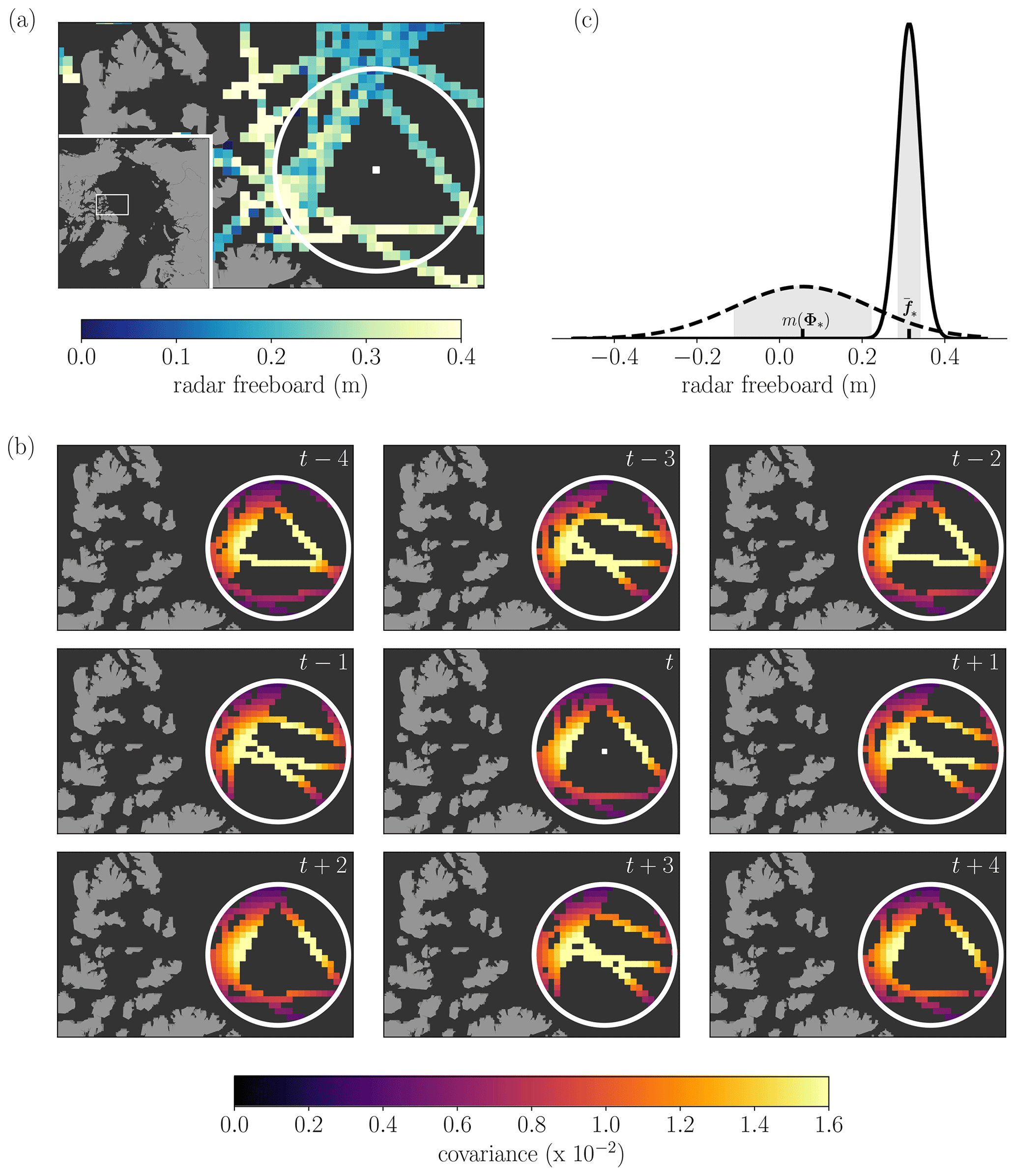
Figure 2Estimating freeboard for one grid cell. (a) In this case we want to estimate a posterior distribution of freeboard values at the location of the white pixel on day t. The white circle corresponds to a distance of 300 km from the pixel, and the gridded tracks are the CS2 and S3 observations on day t. (b) The prior covariance , which is the covariance between the test input Φ* (the white pixel), and all the training inputs Φ that lie within a 300 km radius, for each of the 9 d of training data. (c) Probability density functions showing the prior distribution of function values (dashed), with mean m and 1 standard deviation m, as well as the posterior predictive distribution (solid) showing the estimated freeboard value at the location of the white pixel on day t as m, with 1 standard deviation of m.
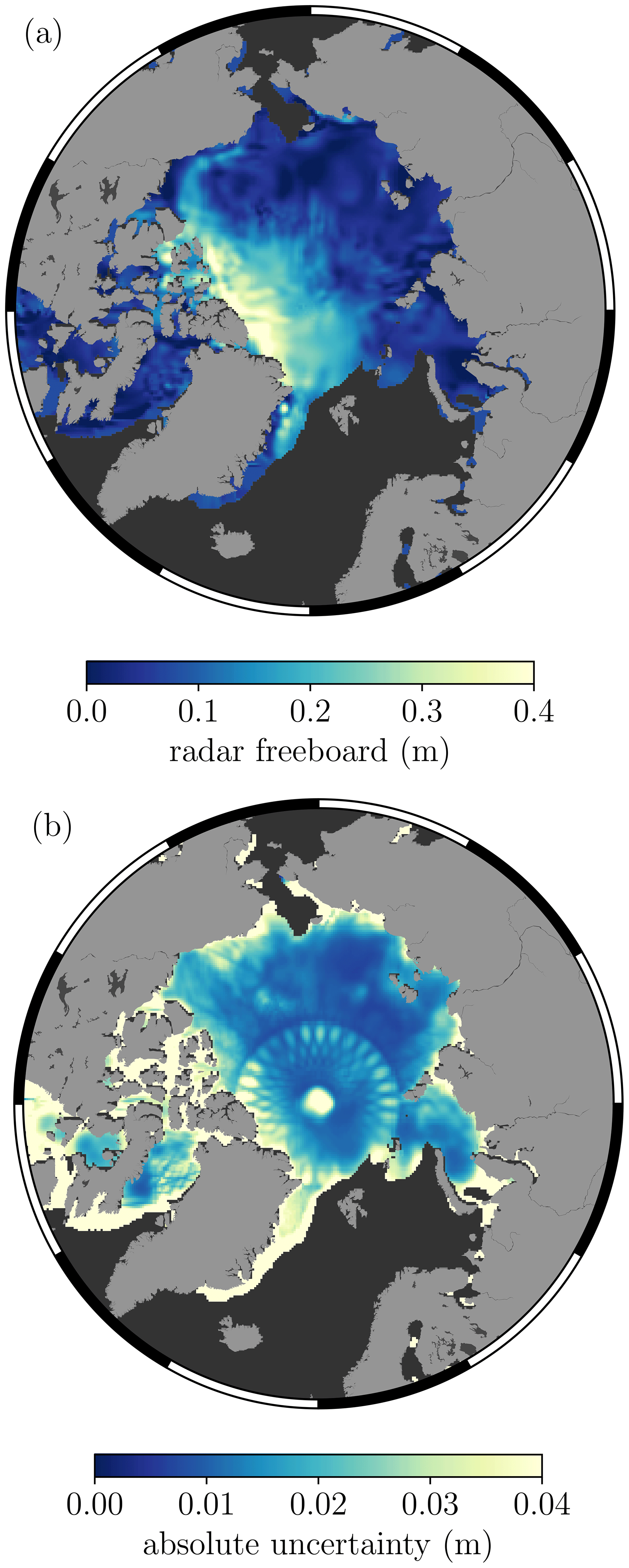
Figure 3(a) Gridded CS2S3 radar freeboard from Gaussian process regression. (b) The absolute uncertainty (1 standard deviation), corresponding to the square root of the predictive variance from Eq. (5). Both images correspond to estimates on the 1 December 2018, at a grid resolution of 25×25 km.
Figure 3 shows the result of repeating the steps in Fig. 2 for every grid cell which contains sea ice on day t. The freeboard values here correspond to the mean of the posterior distribution , and the uncertainty as the square root of the variance term . Notice that the CS2S3 freeboard appears smoother than if we were to simply average the training observation points (e.g. Fig. 1e). This is because GPR estimates the function values f, while we have stated in Eq. (1) that the observations z are the function values corrupted by random Gaussian noise. We also notice how the uncertainty in our estimation of the freeboard values increases in locations where we have fewer training data and is typically highest in areas where we have no data at all (e.g. the polar hole above 88∘ N). In Sect. 5 we provide further discussion relating to the predictive uncertainty of the CS2S3 field, looking particularly at the Canadian Archipelago and the Greenland, Iceland and Norwegian seas, where uncertainties are consistently higher than in other regions of the Arctic. See also Supplement Figs. S1–S2 for sensitivity tests, where we show how the predictions and uncertainty estimates in Fig. 3 are affected by varying the number of days of observations used to train the model.
As a final point related to the methodology, given that we generate the predictions iteratively, we are therefore able to construct daily spatial maps of each of the model hyperparameters that maximise the log marginal likelihood function in Eq. (4). Of particular importance are perhaps the correlation length scale parameters, as these could be of use in other applications such as localisation techniques in sea ice data assimilation systems (Sakov and Bertino, 2011; Massonnet et al., 2015; Zhang et al., 2018, 2021). Previous studies have estimated the average spatial length scales of sea ice thickness anomalies across a range of coupled climate models (Blanchard-Wrigglesworth and Bitz, 2014) and reanalysis products (Ponsoni et al., 2019) to be typically in the range of 500–1000 km. In our approach, the maximum spatial length scales of radar freeboard are capped at 600 km as this is the maximum distance between any pair of grid cells used during the model training (similarly the temporal length scales are capped at 9 d). Nevertheless, from Fig. 4 we notice some interesting features. Specifically, that larger spatial length scales typically coincide with the thicker MYI zone, as well as some localised features around the East Siberian–Chukchi seas and the Kara and Laptev seas. We also see some presence of anisotropy (i.e. at a given pixel, ℓx≠ℓy), particularly in the area north of Greenland, and some regions of the Beaufort Sea. This could be explained by the presence of ridges and other deformation features which form in a preferential orientation relative to the apparent stress regime (Kwok, 2015; Petty et al., 2016). Some of the lowest correlation length scales occur in the peripheral seas, which is perhaps related to more dynamic ice conditions and uncertainty related to spatial sampling in these regions (see Sect. 5 for further discussion). With regards to temporal length scales, we see that radar freeboard observations are correlated over much of the Arctic over the 9 d training period, except for the Canadian Archipelago and some areas of the Greenland, Iceland and Norwegian seas (also discussed further in Sect. 5).
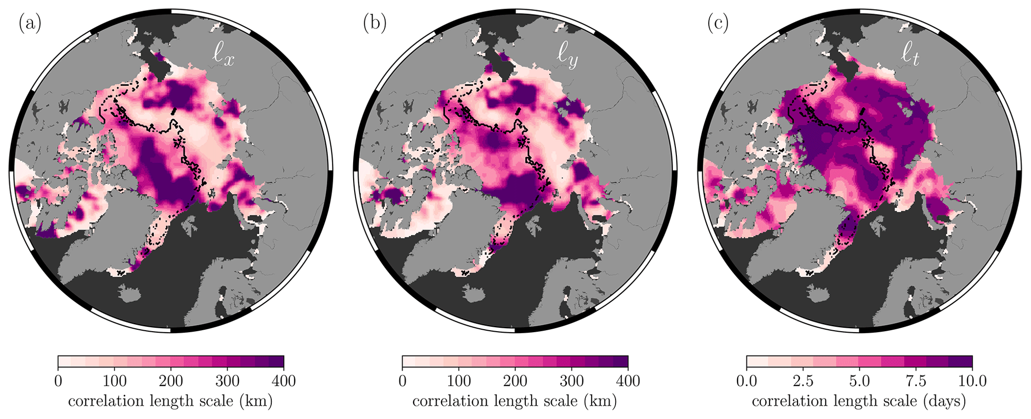
Figure 4The 25×25 km gridded (a) zonal, (b) meridional, and (c) temporal correlation length scales which maximise the log marginal likelihood function (Eq. 4) for the 1 December 2018. The black contour also corresponds to the FYI/MYI contour for the 1 December 2018.
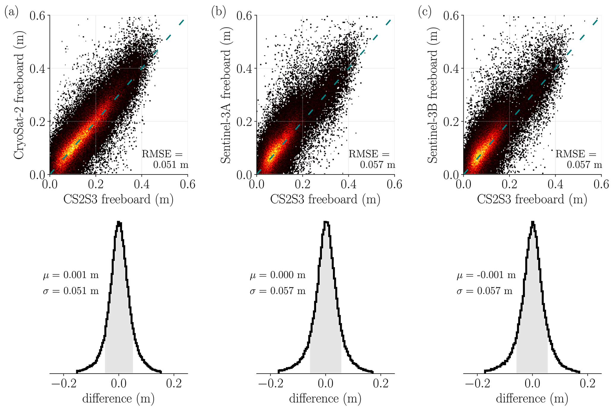
Figure 5Comparison of daily gridded CS2S3 freeboard against daily (a) CS2, (b) S3A, and (c) S3B gridded freeboard tracks, for all days between the 1 December 2018 and the 24 April 2019. In each case, the freeboard values are directly compared in the scatter–density plot (dashed line shows y=x). The distribution of the error is given by the histograms below each scatter plot (1σ either side of the mean μ is shaded in grey). Only values within ±3σ of the mean are shown for the histogram plots.
In this section we use various metrics to assess the GPR model in terms of training and prediction. We first compare CS2S3 daily freeboards against the training inputs in order to derive average errors across the 2018–2019 winter season, before evaluating the predictive performance of the model through cross-validation experiments. Note that hereafter, all CS2S3 fields are generated at 50×50 km resolution, and CS2 and S3 along-track data are averaged to the same 50×50 km polar stereographic grid, for computational efficiency.
4.1 Comparison with training inputs
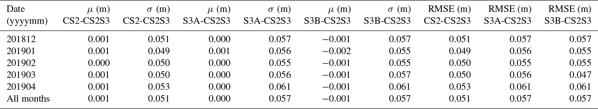
Here we assess the performance of the GPR model during training; that is, an assessment of the errors between the gridded CS2S3 field and CS2 and S3 gridded tracks, for all days between the 1 December 2018 and the 24 April 2019. In general, caution should be applied when evaluating training performance, as a model which fits the training data well may be fitting to the noise in the observations (over-fitting), leading to poor predictive performance. Meanwhile, a model which under-fits the training data is equally undesired (note however that over-fitting is inherently mitigated in the GPR methods; see, e.g., Bishop, 2006). In Eq. (1) we expressed that in our model the freeboard observations from CS2 and S3 correspond to the function values plus random Gaussian noise. Therefore by comparing our CS2S3 freeboard values from Eq. (5) to the training data, we should expect the difference to correspond to zero-mean Gaussian noise. In Fig. 5 we compute differences (CS2-CS2S3, S3A-CS2S3, S3B-CS2S3) for all days, where we can see that the difference (error) follows a normal distribution, centred approximately on 0. The average daily difference μ between CS2S3 and CS2 (or S3) is ≤ 1 mm, with standard deviation on the difference σ<6 cm (see also Supplement Fig. S3 where we compare training errors for interpolations run at different spatial grid resolutions for 1 d). Furthermore, we can see that the root mean square error (RMSE) between CS2S3 and the training inputs is equivalent to the standard deviation of the difference, which can only occur when the average bias is approximately 0. Notably, each of the standard deviations is approximately equal to the ∼6 cm uncertainty in 50 km grid-averaged freeboard measurements, determined from a comparison of S3A and S3B data during the tandem phase of operation (see Supplement Fig. S4). A breakdown of average errors for each month is given in Table 1; however it should be noted that rounding is likely to play a role in many of the presented statistics. For example, we can see that the CS2-CS2S3 mean difference for the “all months” case is reported as 0.001 m, and similarly for S3A-CS2S3 we have 0.000 m. If we expand these, we arrive at 0.00078 and 0.00024 m respectively; hence the apparent difference between means CS2-CS2S3 and S3A-CS2S3 is almost halved.
Table 1Mean (μ), standard deviation (σ), and RMSE of the daily difference between gridded CS2, S3A, and S3B tracks and co-located CS2S3 points, for all days between the 1 December 2018 and the 24 April 2019. Also computed for all days in each respective month.
4.2 Cross-validation
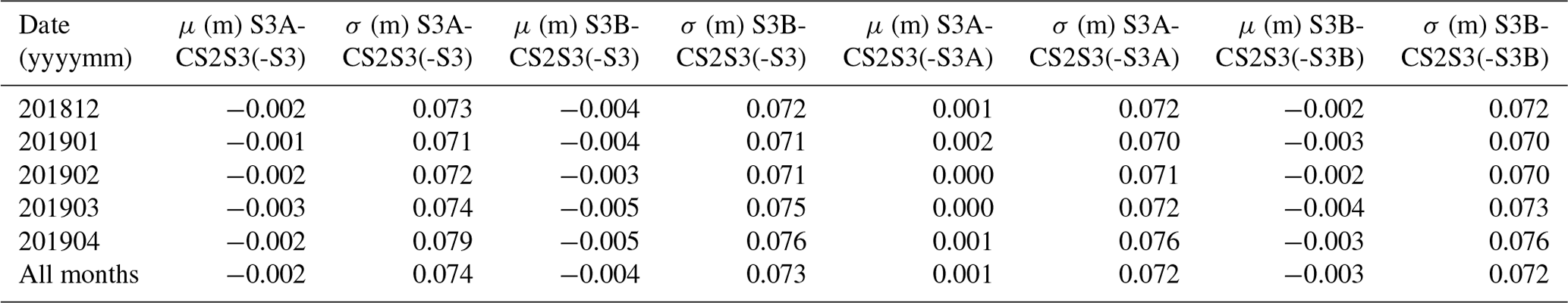
We have seen in the previous section that CS2S3 freeboards closely resemble CS2 and S3 observations (the training data); however this does not give an indication as to how well the model performs in predicting at unobserved locations. An independent set of radar freeboard observations would allow CS2S3 freeboards to be validated at locations unobserved by CS2 or S3 on any given day; however in the absence of these we rely on alternative metrics to evaluate the predictions. Commonly, data from the airborne mission Operation IceBridge are used to validate sea ice freeboard and/or thickness observations; however as only 6 d were collected in a small area around north of Greenland in 2019, there are insufficient data points here to realistically draw any conclusions about the CS2S3 freeboards on larger temporal and spatial scales. K-fold cross-validation is a useful tool when validation data are limited; however models must be run K number of times (ideally where K=n), incurring significant computational expense when n is large (as it is in our case). We opt for a pragmatic solution here: we test the predictive performance of the model by removing different combinations of each of the S3 satellites from the training data, re-generating the predictions with the remaining subset, and subsequently evaluating predictions on the withheld set. For example, in the first instance we generate daily pan-Arctic predictions across the 2018–2019 period, except that we withhold both S3A and S3B from the training set. We then evaluate predictions from each day against observations from S3A and S3B. In the next instance, we repeat the same process except that we withhold only S3A from the training set (whilst retaining S3B) and use S3A as the validation set. In the final scenario, we withhold S3B from the training set and use S3B as the validation set. It should be noted, however, that this approach only allows us to validate predictions below 81.5∘ N and at locations where sea ice concentration values are ≥75 %. This is because 81.5∘ N is the limit of the spatial coverage of S3 satellites, and during the processing of both CS2 and S3 along-track data, diffuse waveforms which sample grid cells with lower than 75 % concentration are discarded (Lawrence et al., 2019). Figure 6 compares predictions for each of the previously mentioned scenarios, across all days in the 2018–2019 winter period. As we would expect, the mean and spread of error in the predictions is largest in the case where only CS2 is used to train the model, with m, σ=0.074 m and m, σ=0.073 m relative to S3A and S3B observations respectively. The mean and spread of error then decreases slightly with the incorporation of either S3A or S3B, with ( m, σ=0.072 m) and ( m, σ=0.072 m) respectively. The mean error across all validation tests is consistently ≤4 mm, showing that the model is able to make reliable predictions at unobserved locations. We can therefore be confident that with the inclusion of all three satellites, the predictions at unobserved locations are at least as good as ≤4 mm error if not better. A breakdown of equivalent statistics is presented for each month in Table 2, although we do not include RMSE here as it is again consistent with the standard deviation in each case. See also Supplement Figs. S5–S6 which show the uplift in the actual predictions and uncertainty estimates brought by the inclusion of all three satellites, as opposed to any one of the cross-validation experiments outlined above.
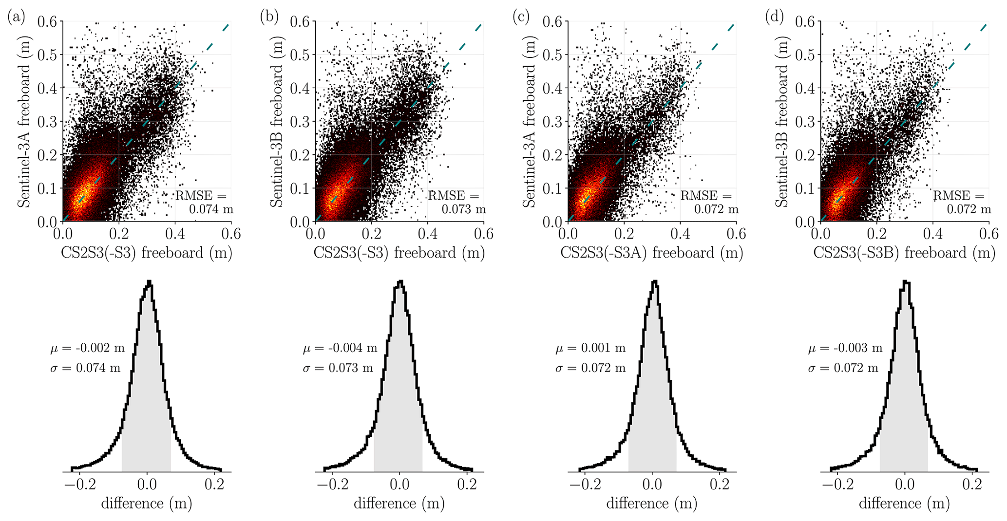
Figure 6Scatter–density plots and error distributions of the GPR predictions for all days between the 1 December 2018 and the 24 April 2019, with different combinations of S3 satellites removed from the training data. (a) Model trained using only CS2 observations, validated against S3A. (b) Model trained using only CS2 observations, validated against S3B. (c) Model trained using only CS2 and S3B observations, validated against S3A. (d) Model trained using only CS2 and S3A observations, validated against S3B. Grey shading is used to indicate 1σ either side of the mean μ for each histogram. Only values within ±3σ of the mean are shown for the histogram plots.
Table 2Mean (μ) and standard deviation (σ) of the daily difference between gridded S3A and S3B tracks and co-located CS2S3 points, with different combinations of S3 observations removed from the training data.
Finally, to showcase the capabilities of the CS2S3 product, we turn to an assessment of temporal variability. Within nine sectors of the Arctic we calculate the mean CS2S3 freeboard for each day of the 2018–2019 winter season to produce a time series of radar freeboard evolution for each sector. We also plot the 31 d running mean freeboard from CS2, S3A, and S3B to demonstrate the increase in variability when moving from a monthly to a daily product. The nine Arctic sectors are taken from NSIDC (Fetterer et al., 2010) and include Baffin and Hudson bays, the Greenland, Iceland and Norwegian (GIN), Kara, Laptev, East Siberian, Chukchi and Beaufort seas, the Canadian Archipelago (CAA), and the central Arctic.
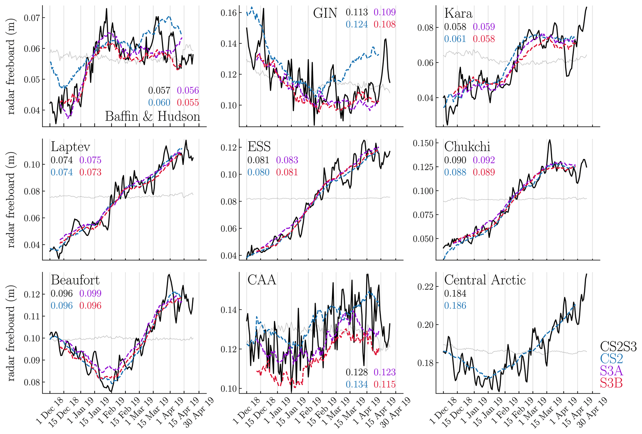
Figure 7Comparison of CS2S3 time series and 31 d running means of CS2 and S3 across nine Arctic sectors. Sectors are defined based on Fetterer et al. (2010) and are available from NSIDC. GIN: Greenland, Iceland, and Norwegian seas; ESS: East Siberian Sea; CAA: Canadian Archipelago. Values presented for each graph correspond to the mean (in metres) of each time series. All means are computed across the period 11 December 2018 to 12 April 2019 (the period where all four time series are available). Note that S3 time series are not included in the central Arctic as much of this region overlaps with the S3 polar hole N. Grey lines are the benchmark time series to test the efficacy of the model (see Sect. 5).
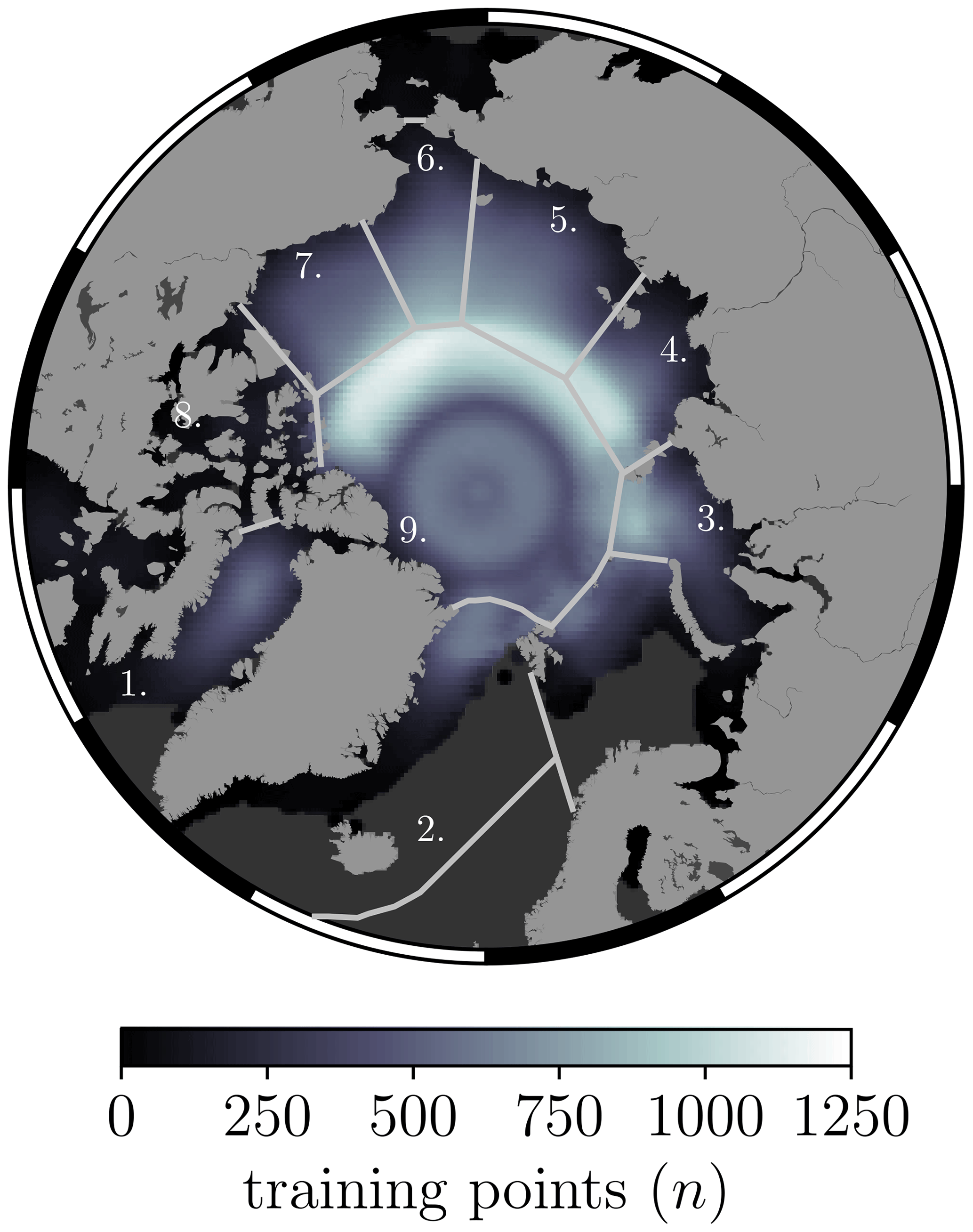
Figure 8The number of training points used to predict radar freeboard at each grid cell at 50×50 km resolution, shown as an average across all days between the 1 December 2018 and the 24 April 2019. The contour lines mark the boundaries between the nine NSIDC regions: (1) Baffin and Hudson bays, (2) Greenland, Iceland, and Norwegian (GIN) seas, (3) Kara Sea, (4) Laptev Sea, (5) East Siberian Sea (ESS), (6) Chukchi Sea, (7) Beaufort Sea, (8) Canadian Archipelago (CAA), (9) central Arctic.
In Fig. 7 we can see how the day-to-day variability is increased with the CS2S3 product, compared to the CS2 and S3 31 d running means. Generally, the mean of the CS2S3 time series lies within 3 mm of CS2 and S3 (approximately in line with the results of the cross-validation presented in Sect. 4.2); however large discrepancies exist in the GIN seas (up to 1.1 cm), the CAA (up to 1.3 cm), and Baffin and Hudson bays (up to 1.2 cm in December 2018). This is perhaps not surprising given the larger uncertainty in radar freeboard in shallow-shelf seas and at coastal margins, relating to higher uncertainty in interpolated sea level anomalies (Lawrence et al., 2019). Indeed, we can see that the difference between the 31 d running means (CS2-S3A(B)) in the CAA is also large, at 1.1 (1.9) cm. The GIN region includes the area east of Greenland, one of the most dynamic regions which carries MYI exported out of the Fram Strait southward. Being such a dynamic region, we expect that the difference in spatial sampling of the three satellites may drive discrepancies between the 31 d running means. Note that the GIN seas, the CAA, and Baffin and Hudson bays also coincide with where we see some of the largest uncertainty in the CS2S3 daily field (e.g. Fig. 3b), as well as the lowest spatial and temporal freeboard correlation length scales (Fig. 4), which may be, in part, a reflection of the discrepancies between CS2 and S3 freeboards in these locations but also due to the limited amount of data available in these regions across the 9 d training period. We can see from Fig. 8 that the number of training points used to provide information on predictions in the coastal margins (including the CAA, GIN seas, and Baffin and Hudson bays) is, on average ≲200 points, whereas in the central regions (central Arctic, Beaufort, Chukchi, East Siberian, Laptev, and Kara seas), the number of training points is typically > 500. A natural question is then whether the variability we see in the time series in Fig. 7 represents a real physical signal or whether it is just noise related to observational uncertainty. To address this question, we first consider the potential issue of spatial sampling by creating a “benchmark” time series (see Fig. 7). For this, we initially compute a “static” background field by averaging all CS2 and S3 gridded tracks between the 1 December 2018 and the 24 April 2019 and then re-generate predictions for each day, as per our GPR model, except that the training data now sample from the background field along the CS2 and S3 track locations of the respective days used in the model training. We should therefore expect the benchmark predictions for each day to be approximately equivalent in areas where there are a significant amount of training data (see Fig. 8) and to see variability in areas where there are less data, which can be explained by tracks sampling different locations of the background field on different days. This is typically what we see in Fig. 7, where there is almost zero day-to-day variability of the benchmark time series in regions such as the Beaufort, Chukchi, East Siberian and Laptev seas but slight variability in the coastal margins. As a second test, we also compare the evolution of daily CS2S3 radar freeboard to daily ERA5 snowfall data, building on the work of Lawrence (2019). Assuming that the radar pulse fully penetrates the sea ice snow cover, radar freeboard is expected to change with snowfall by two distinct mechanisms: (i) snow loading of sea ice will depress the sea ice floe into the ocean, reducing the sea ice freeboard and therefore also the radar freeboard; (ii) because of the slower speed of radar propagation through snow compared to air, additional snowfall will further slow down the pulse, resulting in delayed receipt of the echo at the satellite and equating to a reduced radar freeboard. Thus, under the assumption of full snow penetration, radar freeboard is expected to decrease with increasing snowfall according to these two mechanisms. In Fig. 9 we compute the average of each field over FYI and MYI zones for each day, since surface roughness and snow depth typically show different characteristics over the two ice types (Tilling et al., 2018), and therefore the variability of radar freeboard with snowfall may also show different signals. Freeboard anomalies are then generated by subtracting a second-order polynomial fit to each of the time series. In contrast to expectations, we find a strong positive correlation of 0.52 over FYI and a medium positive correlation of 0.41 over MYI. While it goes beyond the scope of this study to investigate the specific drivers of this correlation, these results appear to challenge conventional assumptions of full snow penetration at Ku-band frequency. Our derived correlation of 0.52 and 0.41, together with our benchmark test, suggest that the CS2S3 data are able to capture physical radar freeboard variability at sub-weekly timescales.
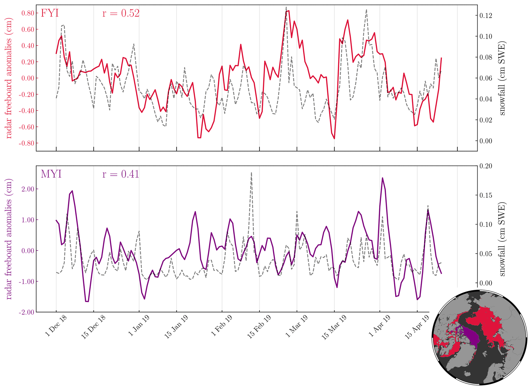
Figure 9Time series of CS2S3 daily radar freeboard anomalies with daily ERA5 snowfall (cm snow water equivalent (SWE)). The corresponding contour for FYI and MYI zones are given in the accompanying spatial plot, where each pixel represents a location which has remained either FYI or MYI for the entire 2018–2019 winter season. The Pearson correlation (r) between radar freeboard anomalies and snowfall are given for each zone.
In this study we presented a methodology for deriving daily gridded pan-Arctic radar freeboard estimates through Gaussian process regression, a Bayesian inference technique. We showed an example of how our method uses 9 d of gridded freeboard observations from CryoSat-2 (CS2), Sentinel-3A (S3A), and Sentinel-3B (S3B) satellites in order to model spatio-temporal covariances between observation points, and make pan-Arctic predictions of radar freeboard, with uncertainty estimates, on any given day at 25×25 km resolution. We refer to this product as CS2S3. We also introduced an empirical Bayesian approach for estimating the (hyper)parameters which define the covariance function, one which maximises the probability of the observations under the choice of model prior and allows us to derive estimates of the spatial and temporal correlation length scales of radar freeboard. An evaluation of the model performance was then carried out for both training and predictions at 50×50 km resolution for computational efficiency. For the training points, we compared our CS2S3 freeboards to gridded CS2 and S3 freeboards at co-located points for all days across the 2018–2019 winter season, where we found the differences to follow a normal distribution, with mean errors ≤ 1 mm and standard deviations <6 cm. We then evaluated the predictive performance of the model for latitudes below 81.5∘ N and at locations where sea ice concentration is ≥75 %, based on a cross-validation approach where we withheld different combinations of S3 freeboards from the training set of observations, re-generated the daily predictions, and used the withheld data to validate the predictions. We found the general prediction error to also be normally distributed, with mean errors ≤4 mm and standard deviations <7.5 cm. Finally, we presented the improved temporal variability of a daily pan-Arctic freeboard product by comparing time series of CS2S3 freeboards, with 31 d running means from CS2 and S3 observations, in nine different Arctic sectors. We showed that the mean of the CS2S3 time series was generally within 3 mm of the 31 d running mean time series from CS2 and S3, except for the Canadian Archipelago and the Greenland, Iceland and Norwegian seas, where prediction uncertainty is large due to significant discrepancies between CS2 and S3 freeboards. We then presented two pieces of analysis to conclude that the variability we see in our radar freeboard time series is related to a real physical signal rather than noise related to observational uncertainty. One is based on a benchmark where we generated predictions from a static field for all days across the 2018–2019 winter season, and for the other we compared time series of daily radar freeboard anomalies to daily ERA5 snowfall data over first-year-ice (FYI) and multi-year-ice (MYI) zones. Pearson correlations between freeboard and snowfall in these regions were given as 0.52 over FYI and 0.42 over MYI, suggesting that the daily fields produced by Gaussian process regression are able to capture real radar freeboard variability. Interestingly, the positive correlation between radar freeboard seemingly contradicts conventional assumptions of full snow penetration at the Ku-band radar frequency and remains the subject of future investigation. The improved temporal variability from a daily product is a hopeful prospect for improving the understanding of physical processes that drive radar freeboard and/or thickness variability on sub-monthly timescales. Of course, an investigation into the drivers of the temporal variability in the CS2S3 field would be an additional way to validate the product, although this goes beyond the scope of our study. We conclude here that the Gaussian process regression method is an extremely robust tool for modelling a wide range of statistical problems, from interpolation of geospatial data sets, as presented here and in other works (Le Traon et al., 1997; Ricker et al., 2017), to time series forecasting (Rasmussen and Williams, 2006; Sun et al., 2014; Gregory et al., 2020). The Gaussian assumption holds well in many environmental applications, and the fact that the Gaussian process prior can take any number of forms, so long as the covariance matrix over the training points is symmetric and positive semi-definite, means that the model can be tailored very specifically to the problem at hand.
Generating the daily CS2S3 radar freeboards at 25×25 km resolution with optimised hyperparameters (as per the methodology outlined in Sect. 3) is computationally demanding and is currently only achieved through high-performance computing systems. We plan to make these open access as and when they become available; however the timings of the release are likely to be governed by the availability of computer resources. It is considerably less burdensome to generate the daily fields without optimisation, by prescribing pre-computed hyperparameter estimates (e.g. a climatology) – we refer to these fields as a “quick-look” product. We find that the quick-look product produces relatively consistent results compared to those presented in Sects. 4 and 5 for the optimised fields, and therefore we will also make these data publicly available.
The code and data files for the optimised and quick-look daily radar freeboards (with uncertainty estimates) can be found in the GitHub repository https://github.com/William-gregory/OptimalInterpolation (last access: 5 May 2021) and Zenodo (https://doi.org/10.5281/zenodo.5005980, Gregory, 2021).
The supplement related to this article is available online at: https://doi.org/10.5194/tc-15-2857-2021-supplement.
WG developed the GPR algorithm and ran the processing for generating the daily CS2S3 fields. IRL conducted all of the pre-processing of CryoSat-2 and Sentinel-3 data files, as well as performing the analysis of the Sentinel-3 tandem phase comparisons. IRL also wrote Sect. 2.1 of this paper. WG wrote the remaining sections. MT suggested the application of the GPR algorithm for this framework of combining satellite altimetry products and also provided technical support and input for writing this paper. Both co-authors contributed to all sections of the paper.
The authors declare that they have no conflict of interest.
Willam Gregory acknowledges support from the UK Natural Environment Research Council (NERC) (grant NE/L002485/1). IRL is supported by NERC through National Capability funding, undertaken by a partnership between the Centre for Polar Observation Modelling and the British Antarctic Survey. Michel Tsamados acknowledges support from the NERC “PRE-MELT” (grant NE/T000546/1) and “MOSAiC” (grant NE/S002510/1) projects and from ESA's “CryoSat+ Antarctica Ocean” (ESA AO/1-9156/17/I-BG) and “EXPRO+ Snow” (ESA AO/1-10061/19/I-EF) projects. The authors wish to thank Jose Manuel Delgado Blasco and Giovanni Sabatino and the entire ESA-ESRIN RSS GPOD Team for carrying out the L0 to L1B satellite data processing. Users of the GPOD/SARvatore family of altimetry processors are supported by ESA funding under the coordination of Jérôme Benveniste (ESA-ESRIN).
The authors would also like to give special thanks to reviewers Alessandro Di Bella and Rachel Tilling for their invaluable insights and feedback throughout the review process.
This paper was edited by John Yackel and reviewed by Rachel Tilling and Alessandro Di Bella.
Aaboe, S., Breivik, L.-A., Sørensen, A., Eastwood, S., and Lavergne, T.: Global sea ice edge and type product user's manual, OSI-403-c & EUMETSAT, 2016. a
Allard, R. A., Farrell, S. L., Hebert, D. A., Johnston, W. F., Li, L., Kurtz, N. T., Phelps, M. W., Posey, P. G., Tilling, R., Ridout, A., and Wallcraft, A. J.: Utilizing CryoSat-2 sea ice thickness to initialize a coupled ice-ocean modeling system, Adv. Space Res., 62, 1265–1280, https://doi.org/10.1016/j.asr.2017.12.030, 2018. a
Balan-Sarojini, B., Tietsche, S., Mayer, M., Balmaseda, M., Zuo, H., de Rosnay, P., Stockdale, T., and Vitart, F.: Year-round impact of winter sea ice thickness observations on seasonal forecasts, The Cryosphere, 15, 325–344, https://doi.org/10.5194/tc-15-325-2021, 2021. a
Bishop, C. M.: Pattern recognition and machine learning, Springer, ISBN 978-0387-31073-2, chap. 3, 152–165, 2006. a
Blanchard-Wrigglesworth, E. and Bitz, C. M.: Characteristics of Arctic sea-ice thickness variability in GCMs, J. Climate, 27, 8244–8258, https://doi.org/10.1175/JCLI-D-14-00345.1, 2014. a
Blockley, E. W. and Peterson, K. A.: Improving Met Office seasonal predictions of Arctic sea ice using assimilation of CryoSat-2 thickness, The Cryosphere, 12, 3419–3438, https://doi.org/10.5194/tc-12-3419-2018, 2018. a
Bushuk, M., Msadek, R., Winton, M., Vecchi, G. A., Gudgel, R., Rosati, A., and Yang, X.: Skillful regional prediction of Arctic sea ice on seasonal timescales, Geophys. Res. Lett., 44, 4953–4964, https://doi.org/10.1002/2017GL073155, 2017. a
Cavalieri, D. J., Parkinson, C. L., Gloersen, P., and Zwally, H. J.: Sea ice concentrations from Nimbus-7 SMMR and DMSP SSM/I-SSMIS passive microwave data, version 1. NASA Natl. Snow and Ice Data Cent, Distrib. Active Arch. Cent., Boulder, Colo., https://doi.org/10.5067/8GQ8LZQVL0VL, 1996. a
Chevallier, M. and Salas-Mélia, D.: The role of sea ice thickness distribution in the Arctic sea ice potential predictability: A diagnostic approach with a coupled GCM, J. Climate, 25, 3025–3038, https://doi.org/10.1175/JCLI-D-11-00209.1, 2012. a
Collow, T. W., Wang, W., Kumar, A., and Zhang, J.: Improving Arctic sea ice prediction using PIOMAS initial sea ice thickness in a coupled ocean–atmosphere model, Mon. Weather Rev., 143, 4618–4630, https://doi.org/10.1175/MWR-D-15-0097.1, 2015. a
Cressie, N. and Johannesson, G.: Fixed rank kriging for very large spatial data sets, J. Roy. Stat. Soc. Ser. B, 70, 209–226, https://doi.org/10.1111/j.1467-9868.2007.00633.x, 2008. a
Day, J., Hawkins, E., and Tietsche, S.: Will Arctic sea ice thickness initialization improve seasonal forecast skill?, Geophys. Res. Lett., 41, 7566–7575, https://doi.org/10.1002/2014GL061694, 2014. a
Dinardo, S., Lucas, B., and Benveniste, J.: SAR altimetry processing on demand service for CryoSat-2 at ESA G-POD, in: Proc. of 2014 Conference on Big Data from Space (BiDS’14), p. 386, https://doi.org/10.2788/854791, 2014. a
Doblas-Reyes, F. J., García-Serrano, J., Lienert, F., Biescas, A. P., and Rodrigues, L. R.: Seasonal climate predictability and forecasting: status and prospects, Wires Clim. Change, 4, 245–268, https://doi.org/10.1002/wcc.217, 2013. a
ERA5: Copernicus Climate Change Service (CDS): Fifth generation of ECMWF atmospheric reanalyses of the global climate, available at: https://cds.climate.copernicus.eu/cdsapp#!/home (last access: 5 August 2019), 2017. a
Fetterer, F., Savoie, M., Helfrich, S., and Clemente-Colón, P.: Multisensor analyzed sea ice extent-northern hemisphere (masie-nh), Tech. rep., Technical report, National Snow and Ice Data Center, Boulder, Colorado USA, https://doi.org/10.7265/N5GT5K3K, 2010. a, b, c
Gregory, W.: William-gregory/OptimalInterpolation: CS2S3 daily pan-Arctic radar freeboards (Version v0.1-quicklook), Zenodo, https://doi.org/10.5281/zenodo.5005980, 2021. a
Gregory, W., Tsamados, M., Stroeve, J., and Sollich, P.: Regional September Sea Ice Forecasting with Complex Networks and Gaussian Processes, Weather Forecast., 35, 793–806, https://doi.org/10.1175/WAF-D-19-0107.1, 2020. a
Guemas, V., Blanchard-Wrigglesworth, E., Chevallier, M., Day, J. J., Déqué, M., Doblas-Reyes, F. J., Fučkar, N. S., Germe, A., Hawkins, E., Keeley, S., Koenigk, T., Salas y Mélia, D., and Tietsche, S.: A review on Arctic sea-ice predictability and prediction on seasonal to decadal time-scales, Q. J. Roy. Meteor. Soc., 142, 546–561, https://doi.org/10.1002/qj.2401, 2016. a
Kang, E. L., Cressie, N., and Shi, T.: Using temporal variability to improve spatial mapping with application to satellite data, Can. J. Stat., 38, 271–289, https://doi.org/10.1002/cjs.10063, 2010. a
Kostopoulou, E.: Applicability of ordinary Kriging modeling techniques for filling satellite data gaps in support of coastal management, Model. Earth Syst. Environ., 7, 1145–1158, https://doi.org/10.1007/s40808-020-00940-5, 2020. a
Kwok, R.: Sea ice convergence along the Arctic coasts of Greenland and the Canadian Arctic Archipelago: Variability and extremes (1992–2014), Geophys. Res. Lett., 42, 7598–7605, https://doi.org/10.1002/2015GL065462, 2015. a
Kwok, R., Kacimi, S., Markus, T., Kurtz, N., Studinger, M., Sonntag, J., Manizade, S., Boisvert, L., and Harbeck, J.: ICESat-2 Surface Height and Sea Ice Freeboard Assessed With ATM Lidar Acquisitions From Operation IceBridge, Geophys. Res. Lett., 46, 11228–11236, https://doi.org/10.1029/2019GL084976, 2019. a
Lawrence, I. R.: Multi-satellite synergies for polar ocean altimetry, PhD thesis, UCL (University College London), 2019. a, b
Lawrence, I. R., Tsamados, M. C., Stroeve, J. C., Armitage, T. W. K., and Ridout, A. L.: Estimating snow depth over Arctic sea ice from calibrated dual-frequency radar freeboards, The Cryosphere, 12, 3551–3564, https://doi.org/10.5194/tc-12-3551-2018, 2018. a
Lawrence, I. R., Armitage, T. W., Tsamados, M. C., Stroeve, J. C., Dinardo, S., Ridout, A. L., Muir, A., Tilling, R. L., and Shepherd, A.: Extending the Arctic sea ice freeboard and sea level record with the Sentinel-3 radar altimeters, Adv. Space Res., 68, 711–723, https://doi.org/10.1016/j.asr.2019.10.011, 2019. a, b, c, d, e, f, g, h, i
Laxon, S., Peacock, N., and Smith, D.: High interannual variability of sea ice thickness in the Arctic region, Nature, 425, 947–950, https://doi.org/10.1038/nature02050, 2003. a
Laxon, S. W., Giles, K. A., Ridout, A. L., Wingham, D. J., Willatt, R., Cullen, R., Kwok, R., Schweiger, A., Zhang, J., Haas, C., Hendricks, S., Krishfield, R., Kurtz, N., Farrell, S., and Davidson, M.: CryoSat-2 estimates of Arctic sea ice thickness and volume, Geophys. Res. Lett., 40, 732–737, https://doi.org/10.1002/grl.50193, 2013. a
Le Traon, P., Nadal, F., and Ducet, N.: An improved mapping method of multisatellite altimeter data, J. Atmos. Ocean. Tech., 15, 522–534, https://doi.org/10.1175/1520-0426(1998)015<0522:AIMMOM>2.0.CO;2, 1997. a, b
Massonnet, F., Fichefet, T., and Goosse, H.: Prospects for improved seasonal Arctic sea ice predictions from multivariate data assimilation, Ocean Modell., 88, 16–25, https://doi.org/10.1016/j.ocemod.2014.12.013, 2015. a
Nolin, A. W., Fetterer, F. M., and Scambos, T. A.: Surface roughness characterizations of sea ice and ice sheets: Case studies with MISR data, IEEE T. Geosci. Remote, 40, 1605–1615, https://doi.org/10.1109/TGRS.2002.801581, 2002. a
Ono, J., Komuro, Y., and Tatebe, H.: Impact of sea-ice thickness initialized in April on Arctic sea-ice extent predictability with the MIROC climate model, Ann. Glaciol., 61, 97–105, https://doi.org/10.1017/aog.2020.13, 2020. a
Paciorek, C. J. and Schervish, M. J.: Spatial modelling using a new class of nonstationary covariance functions, Environmetrics, 17, 483–506, https://doi.org/10.1002/env.785, 2005. a
Petty, A. A., Tsamados, M. C., Kurtz, N. T., Farrell, S. L., Newman, T., Harbeck, J. P., Feltham, D. L., and Richter-Menge, J. A.: Characterizing Arctic sea ice topography using high-resolution IceBridge data, The Cryosphere, 10, 1161–1179, https://doi.org/10.5194/tc-10-1161-2016, 2016. a
Ponsoni, L., Massonnet, F., Fichefet, T., Chevallier, M., and Docquier, D.: On the timescales and length scales of the Arctic sea ice thickness anomalies: a study based on 14 reanalyses, The Cryosphere, 13, 521–543, https://doi.org/10.5194/tc-13-521-2019, 2019. a
Quartly, G. D., Rinne, E., Passaro, M., Andersen, O. B., Dinardo, S., Fleury, S., Guillot, A., Hendricks, S., Kurekin, A. A., Müller, F. L., Ricker, R., Skourup, H., and Tsamados, M.: Retrieving sea level and freeboard in the Arctic: a review of current radar altimetry methodologies and future perspectives, Remote Sensing, 11, 881, https://doi.org/10.3390/rs11070881, 2019. a
Rasmussen, C. and Williams, C. K. I.: Gaussian Processes for Machine Learning, MIT press, ISBN 026218253X, 2006. a, b, c
Ricker, R., Hendricks, S., Kaleschke, L., Tian-Kunze, X., King, J., and Haas, C.: A weekly Arctic sea-ice thickness data record from merged CryoSat-2 and SMOS satellite data, The Cryosphere, 11, 1607–1623, https://doi.org/10.5194/tc-11-1607-2017, 2017. a, b, c, d
Sakov, P. and Bertino, L.: Relation between two common localisation methods for the EnKF, Comput. Geosci., 15, 225–237, https://doi.org/10.1007/s10596-010-9202-6, 2011. a
Sakshaug, E., Bjørge, A., Gulliksen, B., Loeng, H., and Mehlum, F.: Structure, biomass distribution, and energetics of the pelagic ecosystem in the Barents Sea: a synopsis, Polar Biol., 14, 405–411, https://doi.org/10.1007/BF00240261, 1994. a
Schröder, D., Feltham, D. L., Tsamados, M., Ridout, A., and Tilling, R.: New insight from CryoSat-2 sea ice thickness for sea ice modelling, The Cryosphere, 13, 125–139, https://doi.org/10.5194/tc-13-125-2019, 2019. a, b
Schweiger, A., Lindsay, R., Zhang, J., Steele, M., Stern, H., and Kwok, R.: Uncertainty in modeled Arctic sea ice volume, J. Geophys. Res.-Oceans, 116, C00D06, https://doi.org/10.1029/2011JC007084, 2011. a, b, c
Slater, T., Lawrence, I. R., Otosaka, I. N., Shepherd, A., Gourmelen, N., Jakob, L., Tepes, P., Gilbert, L., and Nienow, P.: Review article: Earth's ice imbalance, The Cryosphere, 15, 233–246, https://doi.org/10.5194/tc-15-233-2021, 2021. a
Stirling, I.: The importance of polynyas, ice edges, and leads to marine mammals and birds, J. Marine Syst., 10, 9–21, https://doi.org/10.1016/S0924-7963(96)00054-1, 1997. a
Stroeve, J. and Notz, D.: Changing state of Arctic sea ice across all seasons, Environ. Res. Lett., 13, 103001, https://doi.org/10.1088/1748-9326/aade56, 2018. a
Stroeve, J., Markus, T., Boisvert, L., Miller, J., and Barrett, A.: Changes in Arctic melt season and implications for sea ice loss, Geophys. Res. Lett., 41, 1216–1225, https://doi.org/10.1002/2013GL058951, 2014a. a
Stroeve, J., Barrett, A., Serreze, M., and Schweiger, A.: Using records from submarine, aircraft and satellites to evaluate climate model simulations of Arctic sea ice thickness, The Cryosphere, 8, 1839–1854, https://doi.org/10.5194/tc-8-1839-2014, 2014b. a
Stroeve, J., Vancoppenolle, M., Veyssière, G., Lebrun, M., Castellani, G., Babin, M., Karcher, M., Landy, J., Liston, G. E., and Wilkinson, J.: A multi-sensor and modeling approach for mapping light under sea ice during the ice-growth season, Front. Marine Sci., 7, 1253, https://doi.org/10.3389/fmars.2020.592337, 2021. a
Sun, A. Y., Wang, D., and Xu, X.: Monthly streamflow forecasting using Gaussian process regression, J. Hydrol., 511, 72–81, https://doi.org/10.1016/j.jhydrol.2014.01.023, 2014. a
Tilling, R. L., Ridout, A., and Shepherd, A.: Near-real-time Arctic sea ice thickness and volume from CryoSat-2, The Cryosphere, 10, 2003–2012, https://doi.org/10.5194/tc-10-2003-2016, 2016. a
Tilling, R. L., Ridout, A., and Shepherd, A.: Estimating Arctic sea ice thickness and volume using CryoSat-2 radar altimeter data, Adv. Space Res., 62, 1203–1225, https://doi.org/10.1016/j.asr.2017.10.051, 2018. a, b, c
Wagner, P. M., Hughes, N., Bourbonnais, P., Stroeve, J., Rabenstein, L., Bhatt, U., Little, J., Wiggins, H., and Fleming, A.: Sea-ice information and forecast needs for industry maritime stakeholders, Polar Geogr., 43, 160–187, https://doi.org/10.1080/1088937X.2020.1766592, 2020. a
Zhang, J. and Rothrock, D.: Modeling global sea ice with a thickness and enthalpy distribution model in generalized curvilinear coordinates, Mon. Weather Rev., 131, 845–861, https://doi.org/10.1175/1520-0493(2003)131<0845:MGSIWA>2.0.CO;2, 2003. a
Zhang, Y.-F., Bitz, C. M., Anderson, J. L., Collins, N., Hendricks, J., Hoar, T., Raeder, K., and Massonnet, F.: Insights on sea ice data assimilation from perfect model observing system simulation experiments, J. Climate, 31, 5911–5926, https://doi.org/10.1175/JCLI-D-17-0904.1, 2018. a
Zhang, Y.-F., Bushuk, M., Winton, M., Hurlin, B., Yang, X., Delworth, T., and Jia, L.: Assimilation of Satellite-retrieved Sea Ice Concentration and Prospects for September Predictions of Arctic Sea Ice, J. Climate, 34, 2107–2126, https://doi.org/10.1175/JCLI-D-20-0469.1, 2021. a