the Creative Commons Attribution 4.0 License.
the Creative Commons Attribution 4.0 License.
 | 24 Jun 2021
Estimating subpixel turbulent heat flux over leads from MODIS thermal infrared imagery with deep learning
Zhixiang Yin
Xiaodong Li
Yong Ge
Cheng Shang
Xinyan Li
Yun Du
The turbulent heat flux (THF) over leads is an important parameter for climate change monitoring in the Arctic region. THF over leads is often calculated from satellite-derived ice surface temperature (IST) products, in which mixed pixels containing both ice and open water along lead boundaries reduce the accuracy of calculated THF. To address this problem, this paper proposes a deep residual convolutional neural network (CNN)-based framework to estimate THF over leads at the subpixel scale (DeepSTHF) based on remotely sensed images. The proposed DeepSTHF provides an IST image and the corresponding lead map with a finer spatial resolution than the input IST image so that the subpixel-scale THF can be estimated from them. The proposed approach is verified using simulated and real Moderate Resolution Imaging Spectroradiometer images and compared with the conventional cubic interpolation and pixel-based methods. The results demonstrate that the proposed CNN-based method can effectively estimate subpixel-scale information from the coarse data and performs well in producing fine-spatial-resolution IST images and lead maps, thereby providing more accurate and reliable THF over leads.
- Article
(3082 KB) - Full-text XML
- BibTeX
- EndNote


Leads form a linear area of the open water and thin floating ice within closed pack ice (Willmes and Heinemann, 2015). They arise as a result of various forces, such as thermal stress and wave action (Tschudi et al., 2002). Through leads, the sea surface contacts the atmosphere, thus allowing direct exchange of sensible and latent heat flux (Marcq and Weiss, 2012). Although leads constitute a relatively small percentage of the total sea ice area in the polar regions, they are the primary window for the turbulent heat flux (THF) because the sea ice significantly reduces the air–sea interaction (Maykut, 1978). In the central Arctic region, leads constitute no more than 1 % of sea area during winter but provide a channel for more than 70 % of the upward heat flux (Marcq and Weiss, 2012; Maykut, 1978). Additionally, it has been revealed that small changes in leads can cause a considerable temperature change in a region near the ice surface (Lüpkes et al., 2008). Consequently, the estimation of THF over leads is crucial for studying the climate (Maykut, 1978; Ebert and Curry, 1993).
Remotely sensed satellite images are a promising data source that has been often used in estimating the THF over leads (Qu et al., 2019) because in situ measurement is always difficult to conduct due to harsh weather conditions typical in polar regions. To calculate the THF over leads using the remotely sensed data, both a lead map and the corresponding ice surface temperature (IST) are required (Aulicino et al., 2018). A lead map can be obtained from various satellite data, including visible, thermal, and microwave images (Lindsay and Rothrock, 1995; Röhrs and Kaleschke, 2012; Willmes and Heinemann, 2015). Once a lead map has been generated, the corresponding IST image needed to estimate the THF is commonly derived from the thermal infrared (TIR) bands of satellite data.
Therefore, satellite TIR imagery is essential for the estimation of the THF occurring over leads because it can be used to generate a lead map and the corresponding IST image simultaneously. Thermal infrared images can be obtained from Landsat-8 and Moderate Resolution Imaging Spectroradiometer (MODIS) products. A Landsat-8 TIR image has a spatial resolution of 100 m. However, the Landsat-8 satellite has a revisit cycle of approximately 16 d, making it challenging to estimate THF at appropriate timing. In contrast, MODIS has a daily repeat frequency, which is attractive for studying rapid variations in the THF over leads. However, a MODIS image has a spatial resolution of 1 km and includes mixed pixels. The problem of mixed pixels in MODIS images not only strongly affects the extraction of a lead map but also affects the estimation accuracy of the lead surface temperature, which can result in a large error when calculating THF.
The mixed pixel problem of MODIS TIR images can be solved by conducting a subpixel analysis (Ge et al., 2009; Atkinson, 2013; Ge et al., 2019; Foody and Doan, 2007; Wang et al., 2014; Zhong and Zhang, 2013). The image super-resolution (SR), which aims to enhance the spatial resolution of images, is a representative subpixel-scale analysis method that has been widely used in a variety of applications, including satellite images pan-sharpening (Lanaras et al., 2018), surface topography measurement (Leach and Sherlock, 2013), and land cover mapping (Ling et al., 2010; Foody et al., 2005), and many image SR-based approaches have been proposed (Wang et al., 2020; Glasner et al., 2009). Among them, convolutional neural network (CNN) methods have provided significantly improved performance in producing SR images due to their ability to model a nonlinear relationship between the input and output data (Dong et al., 2014; Ledig et al., 2017). Specifically, in these methods, first, the relationship between an image with a fine spatial resolution and the corresponding image with a coarse spatial resolution is established through the training process with a large amount of training data, and then the trained model is used to super-resolve the testing coarse-spatial-resolution image. These methods have been successfully applied to the SR of sea surface temperature (SST) imagery (Ping et al., 2021) and SR mapping of land cover (Ling and Foody, 2019; Ling et al., 2019; Jia et al., 2019). Therefore, the CNN-based SR methods have great potential in the field of image downscaling, especially fine-spatial-resolution IST images and lead maps that are useful in THF estimation. To the best of the authors' knowledge, a CNN-based method for estimation of the THF occurring over leads has not been reported yet.
This study proposes a CNN-based method for a subpixel-scale estimation of the THF from MODIS TIR images named the deep-learning-based subpixel THF estimation (DeepSTHF) method. Specifically, the DeepSTHF method uses two CNNs to simultaneously produce a Landsat-like IST image and the corresponding binary map of leads from the MODIS IST images, and then it employs the generated Landsat-like IST image and lead map to estimate the THF over leads using an aerodynamic bulk formula (Marcq and Weiss, 2012; Qu et al., 2019; Renfrew et al., 2002). This study provides a new perspective for solving the mixed pixel problem in THF estimation from remotely sensed images by extracting subpixel-level information.
2.1 Study area
The Beaufort Sea, a marginal sea of the Arctic Ocean situated north of Canada and Alaska, was selected as a study area, and it is shown in Fig. 1. The typically severe climate of the Beaufort Sea keeps the sea surface frozen most of the year. However, multiple forces, such as the anti-cyclonic motion of the Beaufort Gyre, cause the ice pack to fracture (Lewis and Hutchings, 2019), generating linear cracks (leads). In addition, global warming has been causing the multi-year ice pack to shrink rapidly (Barber et al., 2014). As a consequence, the size and spatial extent of leads in the Beaufort Sea have been increasing, and various floes along with leads of varying widths and lengths have arisen in this region (Barber et al., 2014).
2.2 Datasets and preprocessing
The proposed DeepSTHF method uses MODIS IST images as input data to calculate a subpixel-scale THF. Remotely sensed images obtained from the Landsat-8 Operational Land Imager (OLI) were used as fine-resolution data to train the two CNN models and to assess the accuracy of the output result. Additionally, associated meteorological data (i.e., wind speed, air temperature, and dew point temperature) were obtained as well to estimate the THF occurring over leads.
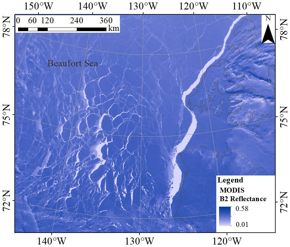
Figure 1Location of the study area. The background image is the band 2 (B2) reflectance of a MODIS image acquired on 25 April 2015. The light-colored area represents leads.
2.2.1 MODIS data
The National Snow and Ice Data Center (NSIDC) provides the MOD29 IST product, wherein all possible cloud-contaminated pixels are removed according to the cloud mask from the MOD35 product. However, upon visual inspection, a number of lead areas with ocean fog or plume (Qu et al., 2019; Fett et al., 1997) can be mistakenly marked as clouds, which can cause a loss of potential leads. Therefore, instead of the MOD29 IST product, the MODIS Level-1B product MOD021KM acquired by the sensor aboard the Terra satellite is used in this study, and it was obtained from the US National Aeronautics and Space Administration's Level 1 and Atmosphere Archive and Distribution System Distributed Active Archive Center (https://ladsweb.modaps.eosdis.nasa.gov/, last access: 22 June 2021). The MOD021KM datasets were stored in the Hierarchical Data Format–Earth Observing System swath structure, which was designed to support archiving and storage of data needed for the Earth Observing System. The MOD021KM dataset mainly contains observational data and geolocation fields. The observation data included 36 calibrated and geolocated spectral bands from the optical region to the TIR wavelength region and had a spatial resolution of 1 km of 1354×2030 pixels. In the MOD02KM data, the cloud contamination area was masked by the cloud masks from the MOD35 product and visual inspection, and pixels with a zenith angle of more than 25∘ were not used to reduce the panoramic bow-tie effect (Eythorsson et al., 2019). The TIR bands 31 and 32, which were respectively centered at 11.03 and 12.02 µm, were used to retrieve the IST using a split-window algorithm (Hall et al., 2001; Key et al., 1994, 1997) that has been adapted to the MODIS data, and whose accuracy has been reported to be within 2 ∘C. Additionally, longitude and latitude coordinates, which were provided in the geolocation field at a 5 km resolution, were used to link the swath to points on the Earth's surface. The MODIS images were collected under the cloud coverage of less than 10 % in the period between March and May from 2013 to 2020 because, during these 3 months, leads are abundant with a variety of sizes and shapes from visual inspection.
2.2.2 Landsat-8 data
This study used the Landsat-8 Level 1 terrain-corrected (L1T) data product acquired from the United States Geological Survey Earth Resources Observation and Science Center from May 2013 to the present. The scenes with the cloud coverage of less than 10 % collected during the period from March to May 2013–2020 were selected.
These Landsat-8 data were used to produce fine-resolution IST reference images and lead maps. The split-window algorithm that was developed for the Landsat-8 data (Fan et al., 2020; Du et al., 2015), and which is suitable for various surface types, including ice and water, was employed to retrieve the IST data. This algorithm estimates temperature from two thermal infrared bands of Landsat-8 data and has an accuracy of better than 1.0 ∘C (Du et al., 2015). It should be noted that the Landsat-8 Thermal Infrared Sensor (TIRS) has a problem with the stray light, which refers to the unwanted radiance from outside the field of view entering the optical system (Montanaro et al., 2015). Nevertheless, certain corrections were made in the current Landsat-8 LIT data product, and the stray light artifact was reduced (Gerace and Montanaro, 2017). However, this artifact was amplified and is thus obvious in the generated IST image, as shown in Fig. 2a, which could impact the estimation accuracy of the THF. A median filtering method (Eppler and Full, 1992; Qu et al., 2019) was used to remove the noise from the Landsat-8 IST image caused by this type of artifact, as shown in Fig. 2b. The reference lead maps were obtained by the iterative threshold method (Qu et al., 2019), and they were manually inspected by referring to the Landsat-8 OLI spectral bands to eliminate possible outliers, as shown in Fig. 2c.
For the obtained Landsat-8 data product, both the OLI spectral bands and the TIRS bands had a pixel size of 30 m. Considering that the TIRS bands at a 30 m resolution were up-sampled from the 100 m raw data using the cubic interpolation to match the OLI spectral bands, the TIRS bands were resampled to 100 m by the average strategy to retain the original spatial resolution.
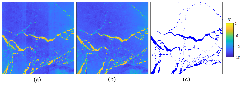
Figure 2The IST images obtained from the Landsat-8 images on 31 March 2020, and the corresponding corrected IST image: (a) the original IST image, (b) the IST image corrected by the median filtering method, and (c) the manually produced lead map. The lead and ice-covered areas are marked as blue and white, respectively.
2.2.3 Meteorological data
Meteorological data included a 10 m wind speed, a 2 m air temperature, and dew point temperature. The meteorological data were taken from the European Centre for Medium-Range Weather Forecasts ERA5 reanalysis hourly dataset (https://cds.climate.copernicus.eu/, last access: 22 June 2021). These data were provided on a 0.25∘ grid and resampled to a 100 m resolution using the cubic interpolation method.
2.2.4 Co-registration of MODIS and Landsat-8 images
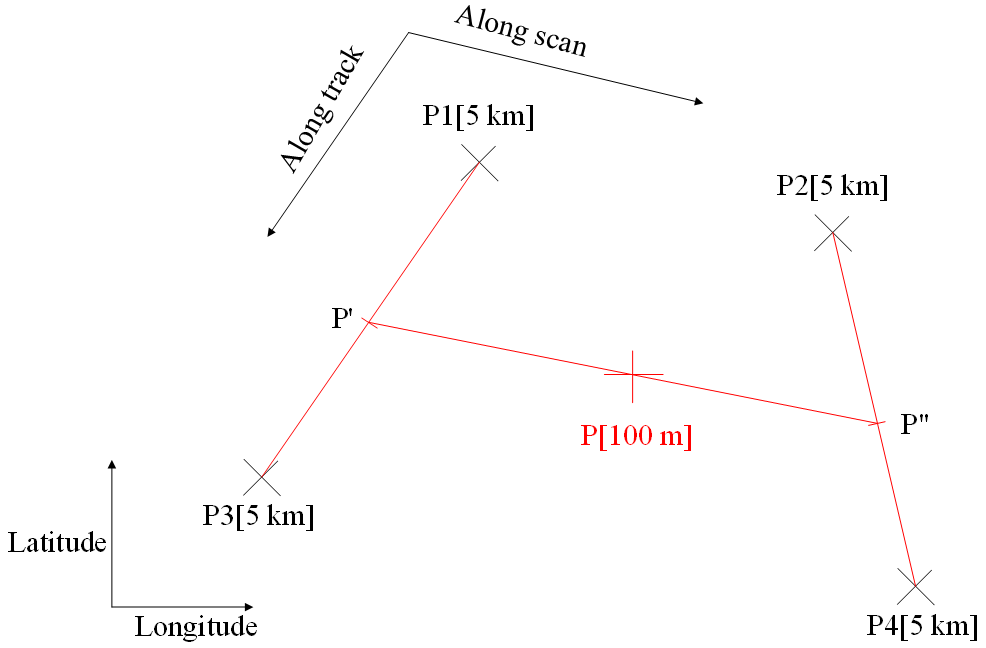
It should be noted that MODIS and Landsat-8 products employ different spatial reference systems; the MOD021KM dataset uses a geolocation subset consisting of longitude and latitude coordinates to provide a geographic location, while Landsat-8 imagery uses a projected coordinate system. Therefore, before being used in the experiment, these datasets were converted to the same spatial reference system. To avoid footprint deviations in different projected coordinate systems and achieve an accurate registration, the Landsat-8 data were transformed into the geolocation data of MOD021KM using the latitude and longitude data. Specifically, the geolocation data of MOD021KM with a 5 km resolution was interpolated to obtain a 100 m resolution geolocation data using a subpixel interpolation strategy. This strategy included three processes, as shown in Fig. 3. First, for a 100 m resolution pixel P to be interpolated, four bounded 5 km resolution pixels P1–P4 were searched. Next, two pixels P′ and P′′ with a 100 m resolution on the along-track line were obtained, and they were on the same along-scan line as pixel P. Then, the longitude and latitude coordinates of pixels P′ and P′′ were interpolated using P1 and P3, and P2 and P4, respectively. The approximation that two successive scan lines were parallel to each other was adopted. Further, the position of pixel P was interpolated with P′/P′′. For each pixel in the interpolated geolocation grid, the corresponding Landsat-8 pixels were obtained using the latitude and longitude coordinates of the grid center. Since points on the ice surface with the same longitude and latitude were identical to each other in different spatial reference systems, the proposed approach can match the coordinates of the different datasets accurately.
The estimation of the THF at a subpixel scale involved two main steps, as shown in Fig. 4. First, a fine-resolution IST image and the corresponding fine-resolution lead map were obtained from a coarse-resolution IST image using a CNN-based integrated method. The CNN-based SR IST reconstruction and lead mapping process included three parts: (1) training data preparation, (2) CNN model training, and (3) prediction of a fine-resolution IST image and lead map using the trained CNN models. Second, the THF was estimated from the fine-resolution IST image and a lead map using an aerodynamic bulk formula, and finally the accuracy of the results was assessed.
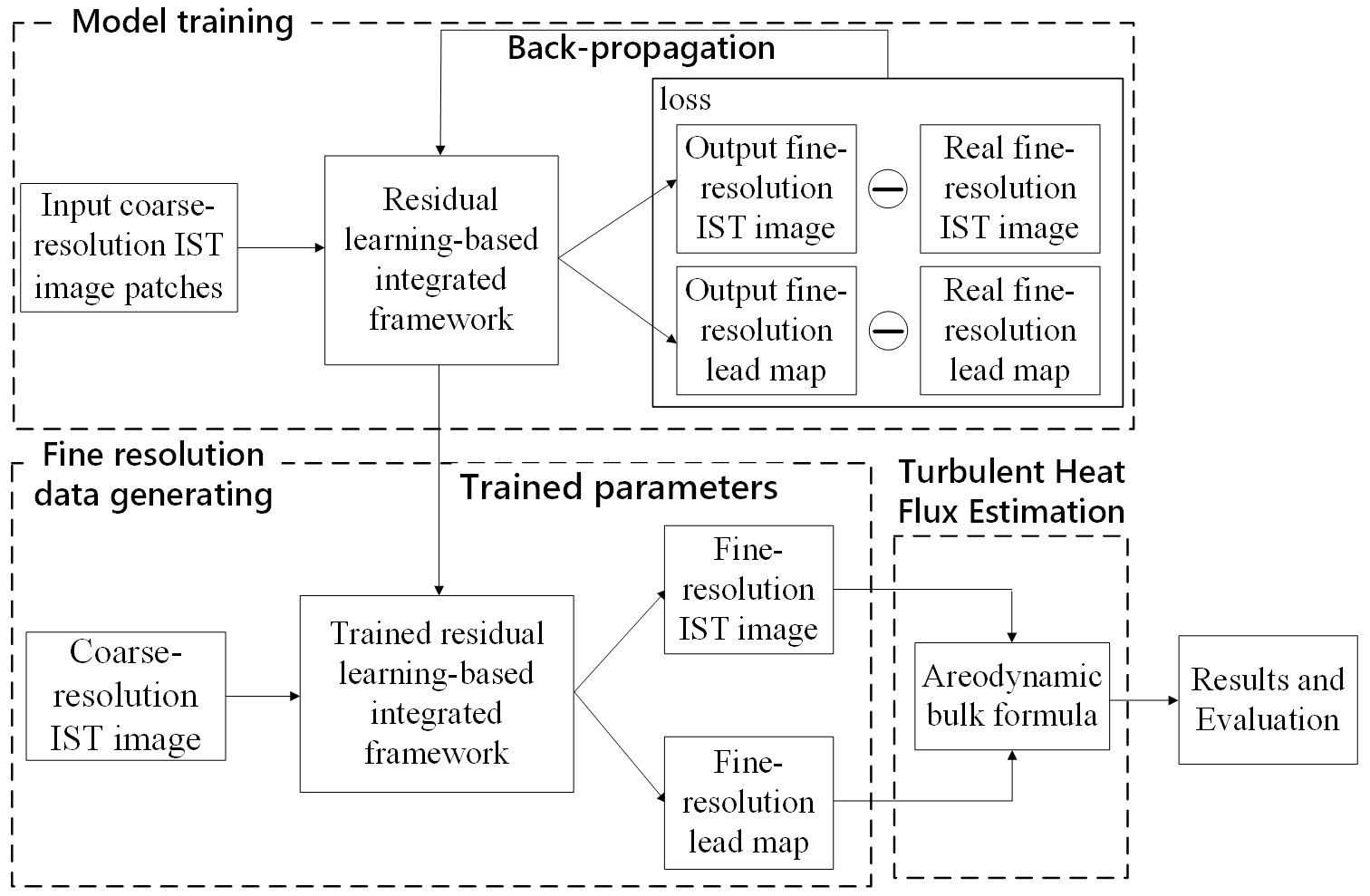
Figure 4The flowchart of the subpixel-scale THF estimation using the proposed deep residual convolutional neural-network-based framework. Note that IST denotes the ice surface temperature.
3.1 Generation of fine-resolution IST image and lead map
Using a coarse-resolution IST image as input, the proposed framework (Fig. 4) aims to produce an IST image and a lead map with finer resolution. Assume that the original coarse-resolution IST image has H×W pixels; then, the objective of the integrated framework is to generate an IST image and a lead map , both of which contain pixels, where z represents the scaling factor, and it equals 10 in this study.
Although the key factors for SR IST image reconstruction and lead mapping both include modeling of a nonlinear relationship between coarse- and fine-resolution data, their objectives are different. The process of generating fine-resolution IST images focuses on recovering a fine spatial pattern, while in the generation of a fine-resolution lead map it is crucial to classify every subpixel in addition to recovering the fine spatial pattern. Therefore, two CNNs with different structures, a very deep residual CNN and a multi-level feature fusion residual CNN, are used in the proposed framework to achieve the generation of a fine-resolution IST image and a lead map, as shown in Fig. 5. The two CNNs are explained in more detail as follows: (1) for fine-resolution IST image reconstruction, a very deep residual CNN, which has been widely used in image SR methods (Zhang et al., 2018b; Ledig et al., 2017), was used (Fig. 5); (2) the SR lead mapping method is essentially a type of image segmentation – considering the good performance of an encoder–decoder structure in image segmentation (Ronneberger et al., 2015; Badrinarayanan et al., 2017), the very deep CNN and encoder–decoder structure were combined, and a multi-level feature fusion residual CNN (Fig. 5) was used for SR lead mapping.
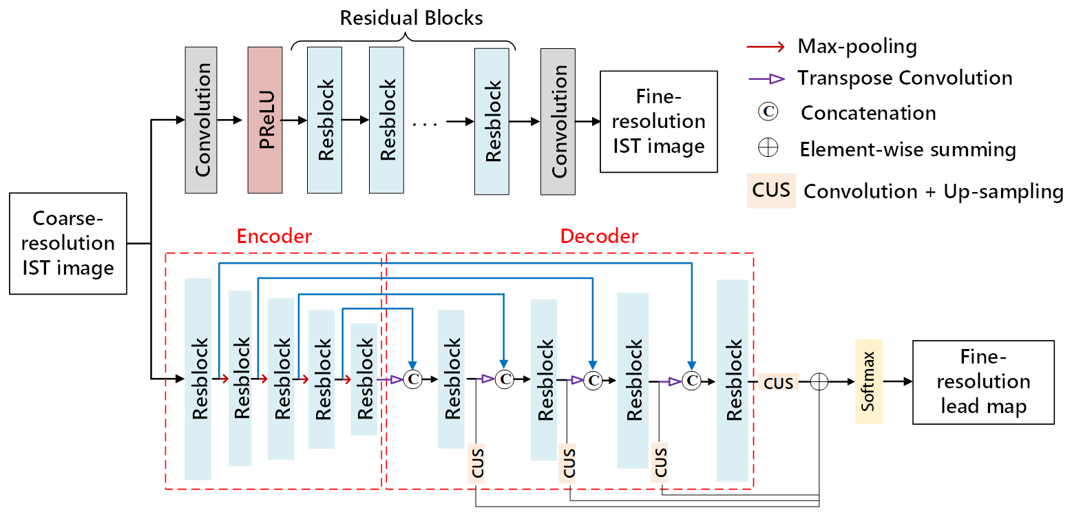
Figure 5Architecture of the two CNNs used for the IST image super-resolution reconstruction and super-resolution lead mapping. Note that PReLU stands for parametric rectified linear unit.
3.1.1 Integrated framework architecture
A very deep residual CNN model with 57 layers was used for SR IST reconstruction. The input coarse IST image was processed by a convolution layer consisting of 64 filters with a size of 3×3 and a parametric rectified linear unit, which was used to ensure the output would be a nonlinear expression of the input data. The core of the very deep residual CNN consisted of nine residual blocks denoted as the “Resblocks”, each of which contained two convolution layers with 64 filters with a size of followed by the batch norm layers and parametric rectified linear unit functions. The last layer of the very deep residual CNN consisted of a single filter.
A multi-level feature fusion residual CNN model was used for SR lead mapping. The model included a symmetric encoder–decoder module and a feature fusion unit. The core of the encoder–decoder also consisted of nine residual blocks. The size of filters in the first convolution layer in each Resblock in the decoder part was , while all other filters in the Resblock had a size of . Additionally, a max-pooling layer, which contained 64 filters with a size of 2×2 and a sliding step of two, was added behind each Resblock in the encoder procedure to downscale the feature maps and to amplify the receptive field. A transpose convolution, which denoted a reverse process to normal convolution (Noh et al., 2015), and a concatenation operation were used in the decoder procedure to enlarge the size of feature maps and to fuse multi-level features, respectively. An attention mechanism module was employed in the concatenation process to increase the feature difference at the boundary of a lead and ice. In the feature fusion part, the features extracted in the decoder part were up-sampled and fused with the element-wise summing to combine multi-level features. The scaling factors of the four up-sampling modules (from left to right in Fig. 5) were eight, four, two, and one, in turn, and they were defined according to the scale differences between the extracted features and the output image. The last layer after the feature fusion part used a softmax function as an activation function to estimate the class label (lead or not lead) of every pixel.
3.1.2 Implementation of CNN models
According to the structures of the CNN models, the input IST image should match the size of the fine-resolution images. Therefore, the coarse-resolution IST images used as training data must be interpolated. A standard interpolation method, the cubic interpolation, was used to process the raw image data to obtain the input dataset. The CNN models were trained using the data consisting of the interpolated coarse-resolution IST image patch x, the corresponding referenced fine-resolution IST image patch y, and lead map patch l. Due to different objectives of image SR IST reconstruction and image SR lead mapping, the mean square error (MSE) loss given by Eq. (1) and the cross-entropy loss given by Eq. (2) were used as loss functions of the two associated CNNs.
In Eqs. (1) and (2), n denotes the number of training samples, F(⋅) denotes the network, w is the weight parameter of the network to be updated in the training process, and the two subscripts correspond to different networks, i.e., SR-IST and SR-LM denote SR of IST and SR of lead mapping, respectively. For optimization, an adaptive moment estimation (Adam) (Kingma and Ba, 2014) with standard backpropagation was applied to minimize the loss and update the network weights until convergence; the parameters of Adam were set as follows: β1=0, β2=0.999; the learning rate α was initialized as 10−1.
Once the two networks have been trained, they could be used to generate the fine-spatial-resolution IST images and the corresponding lead maps. During this procedure, the coarse-resolution IST image was fed into the integrated framework. The fine-resolution IST image was directly generated by the SR IST reconstruction CNN, while the output of the SR lead mapping CNN was a lead indicator image. An appropriate threshold was used to binarize the lead indicator image into a lead map according to specific requirements. The threshold value was empirically set to 0.5, meaning that a fine-spatial-resolution pixel in the indicator image exceeding 0.5 would be classified as a lead pixel.
3.2 Estimation of THF over leads
Given a dataset consisting of fine-resolution IST images, the corresponding lead maps, and related meteorological data (10 m wind speed, 2 m air temperature, and dew point temperature), the THF was estimated over every lead using the traditional aerodynamic bulk formula (Brodeau et al., 2017; Goosse et al., 2001; Renfrew et al., 2002). It should be noted that the overall THF included two parts, sensible (Hs) and latent heat fluxes (Hl). According to the bulk formulae, it was assumed that Hs and Hl were mainly determined by the temperature and humidity differences between the leads' surface and atmosphere at a certain height r (the height of 2 m was used in this study), and they were calculated by
where ρ is the air density, cp is the specific heat of air, and Lw is the latent heat of evaporation; they represent constants in the bulk formula; Ur, Tr, and qr represent the air velocity, temperature, and specific humidity, respectively, at a certain height (here, r=2 m); Ts and qs are the surface temperature and specific humidity at the leads' surface, respectively. The vapor pressure at saturation es (in Pa) was used to calculate qs as follows:
where P is the air pressure, and a and b are coefficients; for an open water area, a=7.5 and b=35.86. Equation (6) was also used to estimate specific humidity qr using the dew temperature. It should be noted that air temperature and air velocity provided by the ERA5 reanalysis hourly dataset corresponded to different heights, so the air velocity at a 2 m height was calculated using the logarithmic neutral wind profile equation (Tennekes, 1973) as follows:
where hr is the reference height (2 m in this study), z0 is the momentum roughness length, K is the von Kármán constant (K=0.4), and μ∗ represents the friction velocity; α and β are the Charnock constant and a “smooth flow” constant, respectively, and they were set to 0.018 and 0.11 empirically in this study; ν is the dynamic viscosity of air, and g is the gravitation constant.
Equations (7) and (8) can be solved in an iteration loop using U10 acquired from the ERA5 dataset. Further, the transfer coefficients Csh and Cle can be respectively calculated by
where z0t and z0q denote the roughness lengths for temperature and humidity, respectively, and they can be obtained as follows:
All of the mentioned variables can be acquired or calculated from the IST image and meteorological data. Once Hs and Hl have been calculated, the overall THF can be obtained by adding them together.
3.3 Accuracy assessment
The DeepSTHF output results were compared with those obtained by the cubic-convolution-interpolation-based subpixel-scale method, which is denoted in this work as cubic-convolution-interpolation-based subpixel THF estimation (CubicSTHF), and the pixel-scale method, which is denoted in this work as original image-based THF estimation (OriTHF). In the CubicSTHF method, the coarse-resolution IST image was first super-resolved by cubic interpolation. Then, the resulting super-resolved IST image was used to produce the corresponding lead map with a pixel-based classification approach (Willmes and Heinemann, 2015). Finally, the THF over leads was calculated using the super-resolved IST image and lead map. In the OriTHF method, the THF over leads was estimated using the original coarse-resolution IST image and the corresponding lead map, which was also obtained from the coarse-resolution IST image using the pixel-based approach.
To assess the performance of the proposed DeepSTHF method comprehensively, two experiments using the simulated and real MODIS images were performed. The experiment with the simulated MODIS images was conducted to explore the performances of the DeepSTHF model as well as to avoid the uncertainty due to co-registration and temperature differences between Landsat-8 and MODIS data. The experiment with the real MODIS images was conducted to assess the performance of the DeepSTHF model in practical applications.
4.1 Experiment with simulated MODIS images
In this experiment, the MODIS IST images were obtained from the Landsat-8 IST images using the pixel aggregate method and were used as the input coarse-resolution data. The original Landsat-8 IST images and the corresponding lead maps were used as the fine-resolution data and as a reference.
4.1.1 Training and test data
The training data of the CNN models were generated from the IST images and lead maps derived from 10 Landsat-8 images acquired during the period of 2013–2017. The IST images and lead maps were clipped into image patches, each of which had a size of 80×80 pixels; the sliding size in the clipping process was set to 40. The clipped IST image patches were degraded to 1000 m to simulate the MODIS IST images. A total of 36 000 image patches, consisting of degraded IST image patches, original Landsat-8 IST image patches, and lead map patches, were randomly selected to form the training data. The degraded IST image patches and the corresponding original IST image patches were used to train the SR IST image reconstruction CNN. Similarly, the degraded IST image patches and the corresponding lead map patches were used to train the SR lead mapping CNN.
During the testing process, the IST images and lead maps obtained from the Landsat-8 scene (p071r010) acquired on 31 March 2020 were used. The IST images were degraded to 1000 m and used as the input of the trained CNNs. The original IST images and lead maps were used as real data to validate the results.
4.1.2 Results
The comparison of the simulated coarse-resolution MODIS IST image, the SR IST images obtained by the CubicSTHF and the DeepSTHF, the reference fine-resolution Landsat-8 IST image, and the error images for the coarse-resolution image and SR results are shown in Fig. 6. Note that the overall spatial texture of the output from DeepSTHF is more like the reference Landsat-8 IST image than the coarse-resolution image and that from CubicSTHF. The SR result for CubicSTHF is blurred in lead areas. Although the SR results of the CubicSTHF and DeepSTHF methods are similar to the reference data for areas covered by ice, the DeepSTHF method produced more accurate results in areas with leads. From the error images, the original coarse-resolution IST image has the largest root-mean-square error (RMSE), which is more than twice as much as those of CubicSTHF and DeepSTHF. Even though CubicSTHF generated a smaller number of errors when compared with the coarse-resolution image, the errors in the lead areas were more significant than those of DeepSTHF.
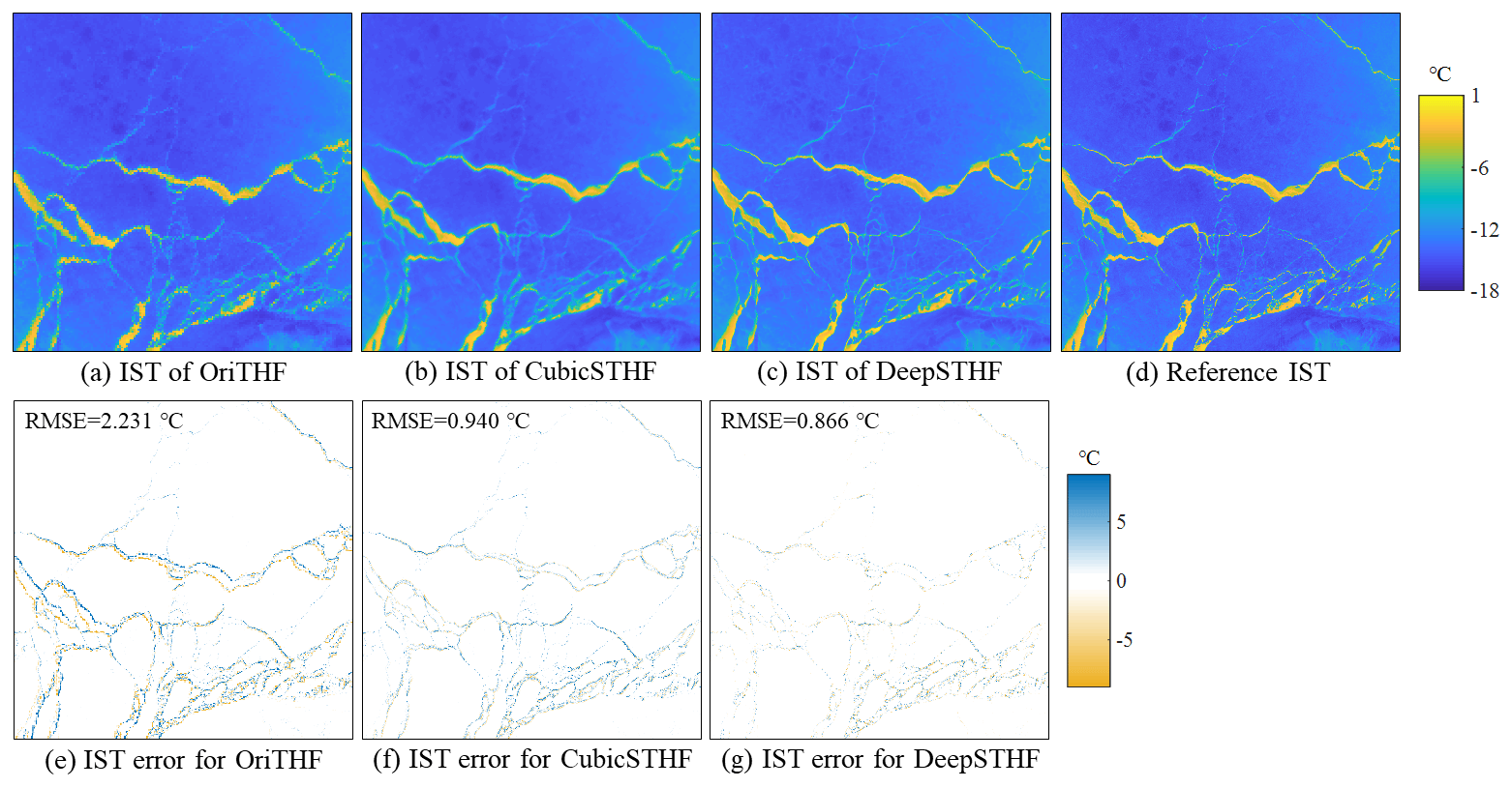
Figure 6Simulated MODIS IST image and SR results of different methods. (a) The IST obtained by the OriTHF; (b) the IST obtained by the CubicSTHF; (c) the IST obtained by the DeepSTHF; (d) the reference IST; (e) the IST error of the OriTHF; (f) the IST error of the CubicTHF method; (g) the IST error of the DeepSTHF method.
The comparison of the scatter plots of the reference IST in generated lead areas and the corresponding IST obtained by a different method, namely, the OriTHF, CubicSTHF, and DeepSTHF methods, is presented in Fig. 7. In the scatter plot corresponding to the OriTHF, the value of r2 was only 0.274, while the values of the CubicSTHF and DeepSTHF methods were significantly higher, indicating a stronger correlation between the SR methods' results and the fine-resolution image. Among the two SR methods, the DeepSTHF has a higher value of r2 but lower RMSE than the CubicSTHF method. Additionally, the results in Fig. 7b show that the CubicSTHF method underestimated most pixels with a reference temperature higher than −6 ∘C, which is indicated by the substantial number of data points below the diagonal line. This problem has been overcome by using the DeepSTHF method. Namely, as shown in Fig. 7c, when the DeepSTHF method was used, the data points are closer to the diagonal line that denotes a 1:1 relationship, and data points are relatively equally located on both sides of the diagonal line in contrast to the other two methods. Thus, the DeepSTHF method achieved the most accurate IST image SR results.
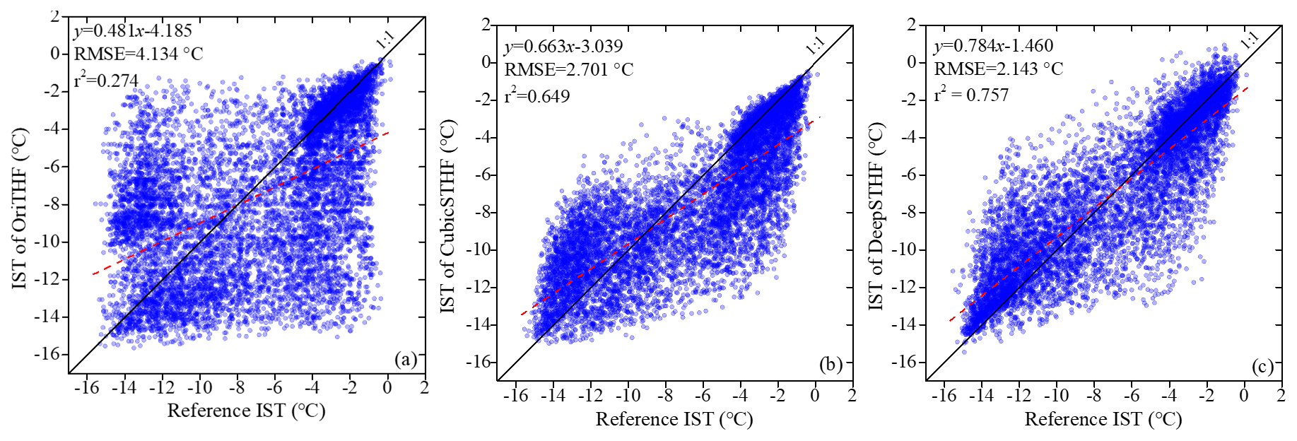
Figure 7Scatter plots of the reference IST in lead areas obtained from the Landsat and the IST obtained by a different method. (a) The OriTHF method; (b) the CubicSTHF method; (c) the proposed DeepSTHF method. The red dashed lines denote fitted linear regression lines of the data points; RMSE and r denote the root-mean-square error and Pearson coefficient, respectively.
The lead maps obtained by the OriTHF, CubicSTHF, and DeepSTHF methods are presented in Fig. 8. The main lead networks generated by the three methods were similar to those in the reference fine-resolution lead map, as shown in Fig. 8c, especially for leads wider than several kilometers. However, the boundaries of the lead maps obtained by the OriTHF were not smooth and not visually realistic. In addition, many narrow lead networks were not extracted by the OriTHF and CubicSTHF, as indicated by the red ellipses in Fig. 8a and b. In contrast, the lead map obtained by the DeepSTHF method was more visually realistic and much closer to the reference lead map. When the DeepSTHF was used, the narrow leads were correctly mapped, and their connectivity was well maintained. It should be noted that some very narrow lead networks in the fine-resolution lead map, especially those with a width of smaller than five pixels, became disconnected when the DeepSTHF method was used, as the red rectangle in Fig. 8c shows; this was because the ice lead fraction in the mixed pixels of the coarse-resolution IST image was too small to provide detailed lead information.

Figure 8Lead maps generated from the simulated IST image using different methods. (a) The lead map generated by the OriTHF method; (b) the lead map generated by the CubicSTHF method; (c) the lead map generated by the DeepSTHF method; (d) the reference lead map extracted from the Landsat-8 operational land imager data. The lead and ice-covered areas are marked in blue and white, respectively. The red ellipses represent lead networks that have not been properly mapped by the OriTHF and CubicSTHF methods, and red rectangles indicate an area with very narrow leads that have not been mapped by the DeepSTHF.
The quantitative assessment of the lead mapping results of the OriTHF, CubicSTHF, and DeepSTHF methods is given in Table 1. The DeepSTHF method had higher overall accuracy and mean intersection over union (MIOU) and a smaller omission error than the OriTHF and CubicSTHF methods. The omission errors for the OriTHF and CubicSTHF methods were 0.341 and 0.240, and they were much greater than that for the DeepSTHF, indicating that many lead pixels were not extracted, which is consistent with the results presented in Fig. 8. In addition, it should be noted that although more lead pixels have been identified by the DeepSTHF method, this did not increase the rate of commission errors. Thus, the DeepSTHF method provided the most accurate lead map among all the methods.
Table 1The lead mapping results of the three methods.

Note that MIOU denotes the mean intersection over union. The most accurate results are highlighted in bold.
Regarding both the IST image SR reconstruction and SR lead mapping, the DeepSTHF method achieved the most accurate results among all the methods. This result is mainly caused by the fact that the CNN-based DeepSTHF model has the ability to extract a potential spatial pattern in the coarse- and fine-resolution IST images/lead maps through learning and built an appropriate nonlinear relationship between them to implement subpixel analysis, which is essential for obtaining reliable SR results. Meanwhile, the CubicSTHF method generated a value for each pixel in the IST image SR result that is a linear combination of surface temperatures of neighboring pixels, which makes it difficult to represent a complex nonlinear relationship between fine- and coarse-resolution images. Additionally, the threshold approach is used in the CubicSTHF method to extract leads, which is a pixel-based method and cannot achieve subpixel analysis.
The distributions of the THF over leads estimated by the three methods are presented in Fig. 9, where it can be seen that the proposed DeepSTHF method preserved abundant spatial texture and achieved more accurate results than the OriTHF and CubicSTHF methods. Since the OriTHF and CubicSTHF failed to retrieve many small leads, the THF over these leads was not calculated, as shown in Fig. 9a and b, and thus significant errors in the corresponding areas appeared in the error map, as shown in Fig. 9e. Additionally, even though the estimated THFs for large leads obtained by the OriTHF and CubicSTHF were close to the reference data, the obtained THF along boundaries was much lower than the true value, which resulted in large errors, especially for the OriTHF method, as shown in Fig. 9e and f. In contrast, the DeepSTHF has a relatively small overall error.
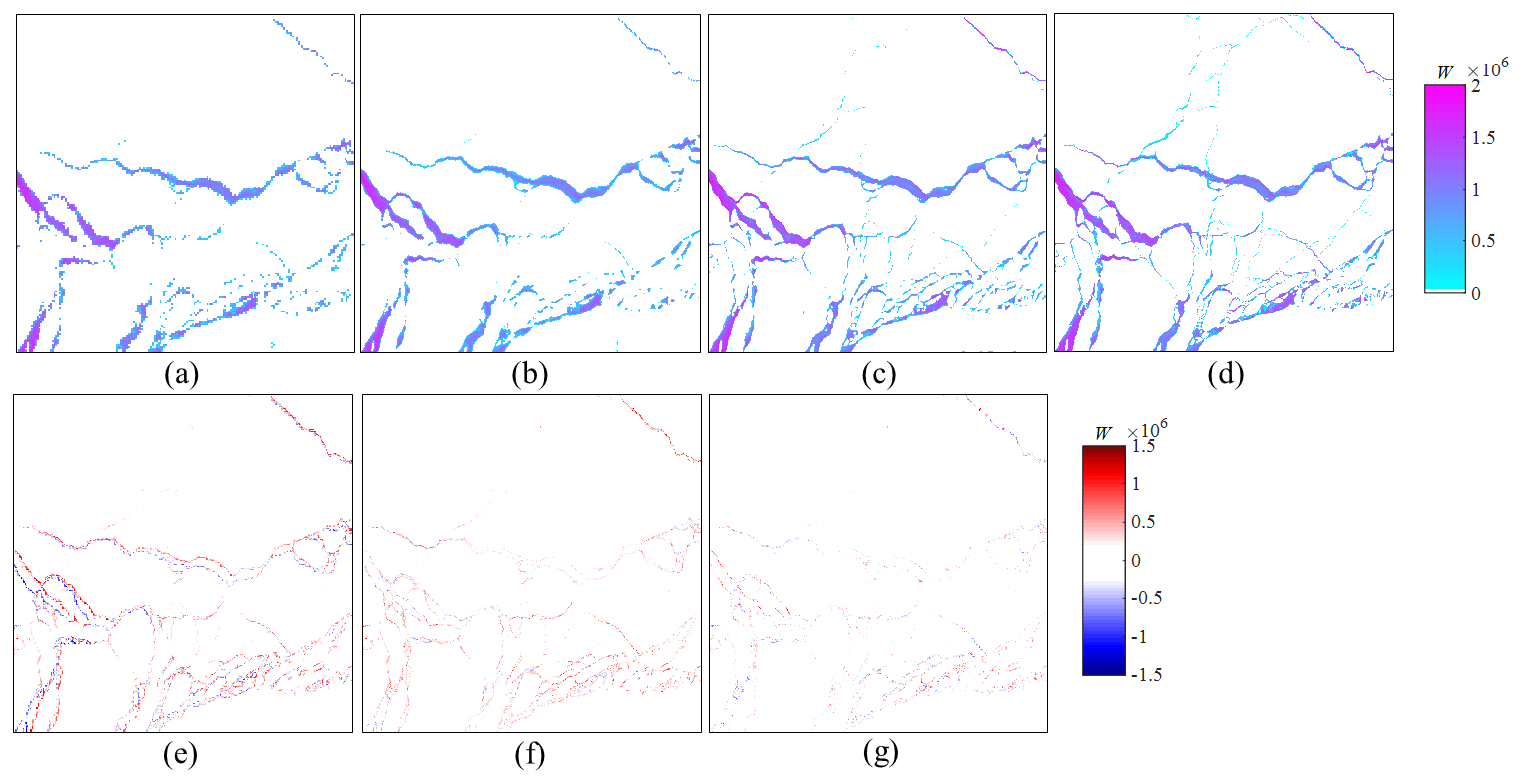
Figure 9Spatial distribution of the THF calculated by different methods: (a) the OriTHF method; (b) the CubicSTHF method; (c) the proposed DeepSTHF method; (d) the reference distribution. The error maps of the distribution of the THF of (e) the OriTHF method, (f) the CubicSTHF method, and (g) the proposed DeepSTHF method.
The scatter plots of the reference THF data plotted against the THF data estimated by the OriTHF, CubicSTHF, and DeepSTHF methods are shown in Fig. 10. Generally, the THF data estimated by the DeepSTHF method were closer to the diagonal line than those estimated by the OriTHF and CubicSTHF methods. Several THF values estimated by the OriTHF and CubicSTHF methods were less than 0.25×10⁶ W. This mainly occurred because small leads were not mapped, so the corresponding THFs were not estimated. The r2 values of the CubicSTHF and DeepSTHF methods were both much higher than that of the OriTHF. Even though the result of the CubicSTHF had a higher correlation with the reference data than that of the OriTHF, it is evident that most of the pixel values were underestimated, as shown in Fig. 10b. It should be noted that, for all plots, there are data points on both vertical and horizontal axes, which was due to the omission (points on the horizontal axis) and misclassification (points on the vertical axis) of lead pixels of the three methods during the lead mapping.

Figure 10Scatter plots of the THF calculated from the reference data and the THF estimated by (a) the OriTHF method, (b) the CubicSTHF method, and (c) the DeepSTHF method. The red dashed lines denote the fitted linear regression lines of the data points. RMSE and r denote the root-mean-square error and Pearson coefficient, respectively.
The total THF estimated by the OriTHF, CubicSTHF, and DeepSTHF methods, as well as the accuracies of all the methods, are listed in Table 2. Generally, the total THF estimated by the DeepSTHF method was the closest to the reference data. Although the THF estimated by the OriTHF was relatively closer to the reference value than that estimated by the CubicSTHF, its RMSE was much larger. In contrast, the THF estimated by the DeepSTHF had the smallest RMSE and overall error (OE) and the greatest r2, especially for the OE. The OE values of the OriTHF and CubicSTHF methods were almost 3 times that of the DeepSTHF method. The THF error (i.e., the real value minus the estimated value) distributions of the three methods are demonstrated in Fig. 11. More than 70 % of all errors of the DeepSTHF method were located in the small error range of [, 0.25×10¹¹ W], while the percentage of errors in this range for the other two methods was much smaller, i.e., less than 50 % for the OriTHF method and less than 60 % for the CubicSTHF method. For the DeepSTHF method, the errors were close to a normal distribution, and the rate of positive errors was close to that of negative errors. Meanwhile, for the CubicSTHF method, the THF of most pixels was underestimated, as shown in Fig. 10; the rate of positive errors was significantly larger than the corresponding negative errors, and the errors were biased. Therefore, compared with the CubicSTHF method, although the improvement of the DeepSTHF method in RMSE was not large, the total estimated THF data were much closer to the reference data because the most positive and negative errors tended to cancel out each other, which was statistically good. These findings indicated that the proposed DeepSTHF method can achieve a more favorable result than the other two methods and can accurately estimate THF over leads at a subpixel scale.
Table 2Accuracies of the estimated turbulent heat flux (THF) estimated by different methods.
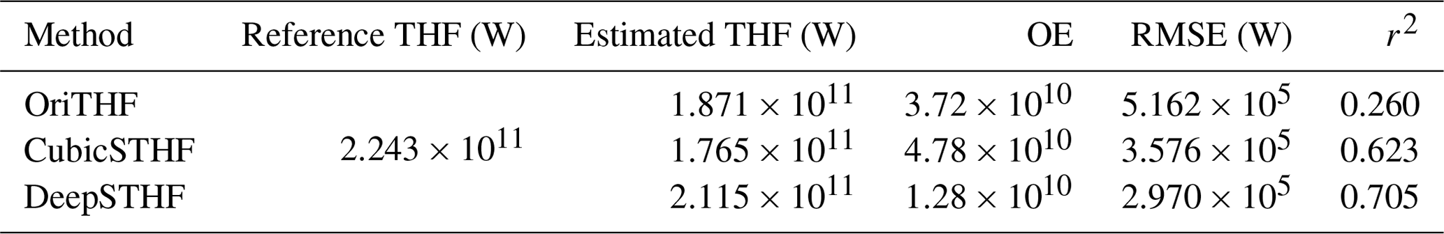
Note that OE stands for the overall error.

4.2 Experiment with real MODIS images
In this experiment, real MODIS images were used to obtain the input coarse-resolution IST images, while the Landsat-8 images were used to produce the reference fine-resolution IST images and lead maps.
4.2.1 Training and test data
Ten MODIS IST images, the corresponding Landsat-8 IST images, and lead maps acquired during the period of 2013–2017 were used to create training samples of the CNN models. The Landsat-8 images were converted to a MODIS geolocation grid to achieve accurate co-registration between the Landsat-8 and MODIS images. Using the same method as in the previous experiment, the images were clipped into image subsets with a size of 80×80 pixels with an overlapping size of 40 pixels between neighboring subsets. The SR IST image reconstruction CNN model and the image SR lead mapping CNN model were trained using a total of 36 000 randomly selected MODIS IST image patches as well as the corresponding Landsat-8 IST image and lead map patches.
Three MODIS IST images acquired on 25 April 2018, 9 May 2019, and 31 March 2020 were used to estimate the THF at a subpixel scale. For each MODIS image, a subset containing leads with different widths and lengths was selected for the experiment. The three corresponding Landsat-8 scenes denoted as p057r010, p111r240, and p071r010 were employed to provide reference fine-resolution data used to validate the results. The generalization ability of the proposed model could be accurately validated because the test images were located in different regions and observed on these dates when leads changed quickly.
It should be noted that there were large temperature differences between the MODIS and Landsat-8 IST images, which was mainly due to different overpass times of the MODIS and Landsat-8 satellites. A possible way to reduce this inconsistency is to use a sinusoid-based temporal correction method (Van Doninck et al., 2011). However, in practice, the temporal correction method can introduce an additional error because the sinusoidal method may not be able to model a complex variation of temperatures. Due to this factor, the MODIS and Landsat-8 IST images were normalized before training by the min–max normalization method. Furthermore, in the test stage, the MODIS IST image SR results were not evaluated quantitatively due to a lack of true fine-resolution IST reference images; they were assessed visually. For lead mapping, it was assumed that the range of leads varied slightly from the MODIS observation time to the Landsat-8 observation time so that the lead maps produced from the Landsat-8 OLI data could be used to validate the SR lead mapping results.
4.2.2 Results
The MODIS IST images and the corresponding image SR reconstruction results of the CubicSTHF and DeepSTHF methods are shown in Fig. 12. A visual assessment of the results of the CubicSTHF and DeepSTHF method shows that these results were more realistic than those of the original MODIS IST images, which were not smooth along the boundaries of the lead networks. Compared with the results of the CubicSTHF method, finer spatial textures were observed in the images obtained by the DeepSTHF. For lead networks, the SR result of the CubicSTHF method was blurred to a certain extent, but it was sharper than that of the DeepSTHF method. The temperature difference between the lead and ice areas along the boundary was more significant in the result of the DeepSTHF method than in that of the CubicSTHF method.

Figure 12The IST images were acquired on (a–c) 25 April 2018, (d–f) 9 May 2019, and (g–f) 31 March 2020. The SR result was obtained by (a, d, g) the OriTHF method, (b, e, h) the CubicSTHF method, and (c, f, i) the proposed DeepSTHF method.
The generated lead maps obtained by the OriTHF, CubicSTHF, and DeepSTHF methods are displayed in Fig. 13. Generally, the lead maps obtained by the DeepSTHF method were more similar to the reference maps than those obtained by the other methods. The OriTHF and CubicSTHF methods failed to identify many narrow leads, which made the corresponding lead networks become disconnected, as red rectangles in Fig. 13b, f, and j show. Some parts of the ice-covered regions surrounded by leads were misclassified as leads by the OriTHF and CubicSTHF methods, as shown in red ellipses in Fig. 13b and j. Even though the main lead networks were correctly mapped by the OriTHF method, the boundaries of the obtained lead networks were jagged, as shown in Fig. 13q and u. The results of the CubicSTHF method were smoother than those of the OriTHF method, but some parts of large lead networks were discontinuous, as shown in Fig. 13r and v, which increased the lead widths in them to a certain extent. In contrast, the proposed DeepSTHF method achieved more promising results. First, it identified most small leads and maintained their connectivity. Second, the boundaries of the segmented leads were smooth and much closer to those of the reference leads (subareas r1–r3). Third, most ice-covered areas surrounded by leads were correctly classified, even when the areas were relatively small, as shown in the dashed red rectangle in Fig. 13k. It should be noted that although the DeepSTHF method extracted most leads accurately, it did not perform well on very narrow leads, especially those with the width of less than 5 pixels in the fine-resolution map from Landsat-8 data because the lead fraction for these leads in the coarse image was too small and could hardly be mapped to the fine-resolution lead map using the CNN model. Additionally, the results of the DeepSTHF method were influenced by abnormal pixels in the input data. For instance, some of the pixels were misclassified in a narrow rectangular area, as shown in the red dashed ellipse in Fig. 13c, because the temperature of this area did not correctly reflect the actual case in the ocean, as displayed in Fig. 12a.
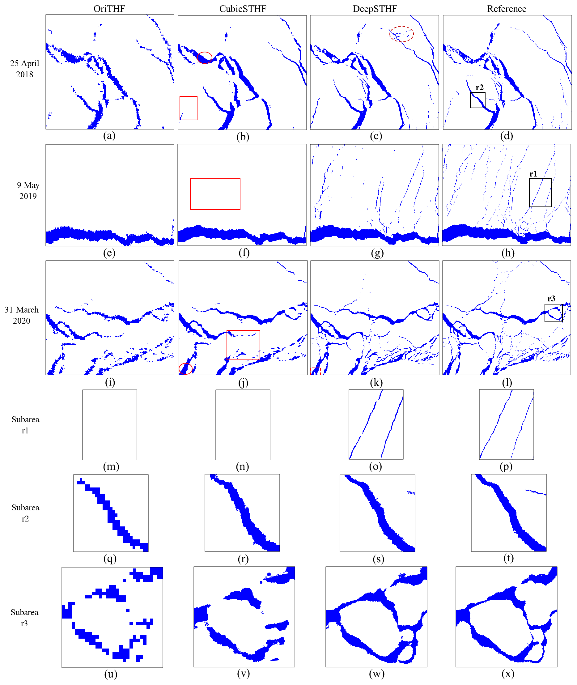
Figure 13The lead maps generated from the MODIS IST images using the three methods. The images were acquired on (a–d) 25 April 2018, (e–h) 9 May 2019, and (i–l) 31 March 2020. The lead and ice-covered areas are marked in blue and white, respectively. (a, e, i, m, q, u) The results of the OriTHF method, (b, f, j, n, r, v) the results of the CubicSTHF method, and (c, g, k, o, s, w) the results of the DeepSTHF method. The black rectangles in panels (d), (h), and (i) represent the subareas. The red rectangles in panels (b), (f), and (j) represent the lead networks that have been mapped by the CubicSTHF method. The red ellipses in panels (b) and (j) show the ice-covered regions that have been misclassified as leads by the CubicSTHF method. The red dashed rectangle in panel (k) represents the ice-covered areas that have been correctly classified by the DeepSTHF method. The red dashed ellipse in panel (c) shows the pixels misclassified as leads by the DeepSTHF method due to the errors in the ice surface temperature.
The quantitative performances of the lead maps generated by the three methods are compared in Table 3. As the results in Table 3 show, the DeepSTHF method provided the highest overall accuracy and MIOU, as well as the lowest commission error, on 25 April 2018 and 31 March 2020. Although the commission error of the DeepSTHF method on 9 May 2019 was higher than those of the OriTHF and CubicSTHF methods, the overall accuracy and MIOU of the DeepSTHF method were larger. The accuracy of the OriTHF method was the lowest except for 9 May 2019. The commission errors of the three methods on 9 May 2019 were small because, in the data collected on this day, the lead areas mainly consisted of a large lead network that could be easily extracted. For all dates, the omission errors of the OriTHF and CubicSTHF methods were much larger than that of the CNN, demonstrating that many lead pixels were not correctly classified, which was consistent with the visual results presented in Fig. 13. Therefore, the proposed framework was also effective in the image SR lead mapping with real MODIS data.
Table 3Accuracies of the lead maps obtained by different methods using data acquired on different dates.
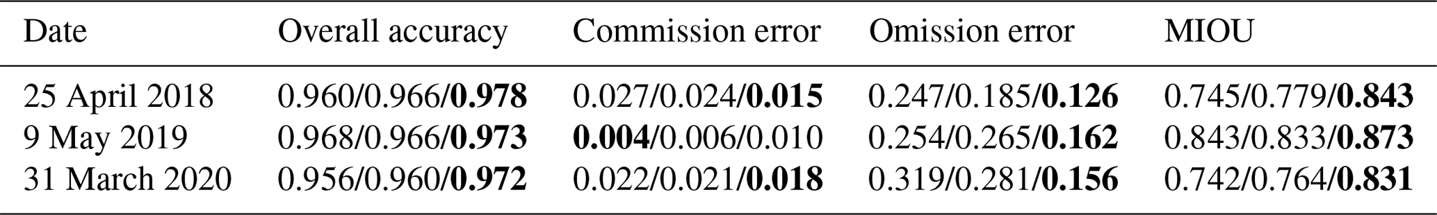
Note that MIOU stands for the mean intersection over union. The given numbers denote the first, second, and third numbers in the entry, respectively. The most accurate results are in bold text.
The THF over mapped leads estimated by the OriTHF, CubicSTHF, and DeepSTHF methods is shown in Fig. 14. Since the estimated THF was dependent on the generated lead maps, the spatial distribution of the estimated THF was consistent with the lead maps. Specifically, in the plots corresponding to the OriTHF and CubicSTHF methods, the THF of most small leads was not depicted, and the lead boundaries were not smooth, especially for the plot corresponding to the OriTHF method. Additionally, the estimated THF of pixels along the boundaries of the lead networks was relatively small for the CubicSTHF method, which could be due to the underestimation of temperature in the SR IST image. Meanwhile, for the DeepSTHF method, the THF over many of the small leads was correctly estimated, and the overall spatial pattern of the estimated THF in the plot was much finer than those of the OriTHF and CubicSTHF methods.
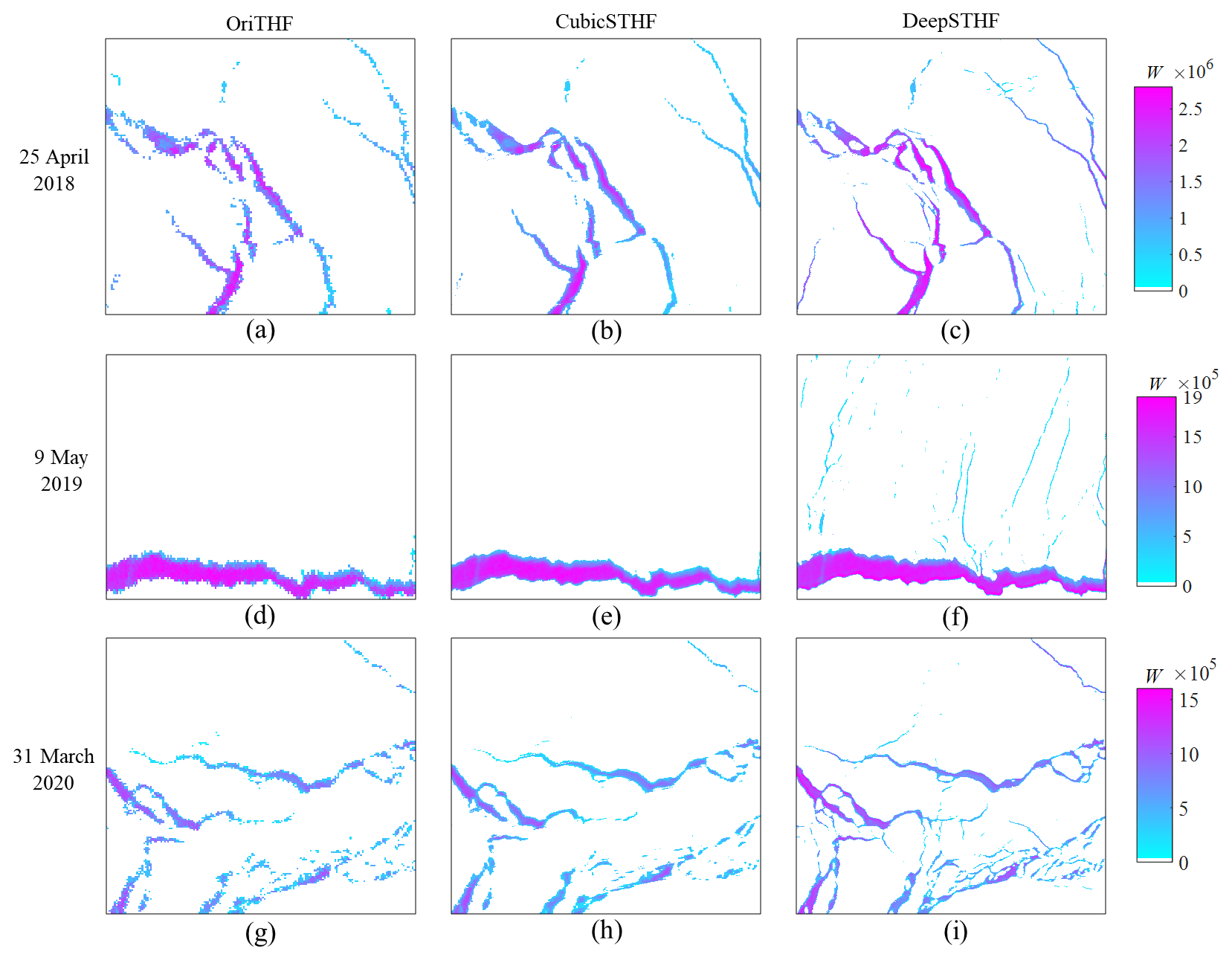
Figure 14Spatial distributions of the THF obtained by (a, d, g) the OriTHF method, (b, e, h) the CubicSTHF method, and (c, f, i) the DeepSTHF method. The data were collected on (a–c) 25 April 2018, (d–f) 9 May 2019, and (g–i) 31 March 2020.
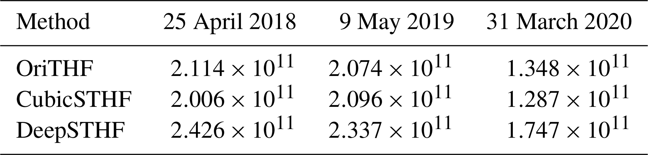
The estimated THFs on different dates obtained by the three methods are given in Table 4. Although more leads were identified using the CubicSTHF method than the OriTHF method on 25 April 2018 and 31 March 2020, which is indicated by a smaller number of omission errors, the THF estimated by the CubicSTHF was slightly smaller than that of the OriTHF method on both dates. This was mainly because the temperature of lead pixels along the lead networks was lower in the SR process by the CubicSTHF method, as shown in Fig. 12. Meanwhile, since for the DeepSTHF method more leads were mapped, and the reconstructed temperature of lead pixels along lead networks was close to the pixels in the central part of lead networks, the total THF obtained by the DeepSTHF method on all dates was greater than those of the OriTHF and CubicSTHF methods. The THF difference between DeepSTHF and the other two methods on 31 March 2020 was the largest, followed by that on 25 April 2018, while that on 9 May 2019 was the smallest. The main reason for this was that the test area on 31 March 2020 comprised many small leads that were not correctly classified by the OriTHF and CubicSTHF, and the test area on 9 May 2019 mainly consisted of a large lead network that was successfully extracted by all three methods, where only a few small lead networks were mapped by the DeepSTHF method, as shown in Fig. 13g. Therefore, the DeepSTHF achieved more accurate results in the areas composed of leads with abundant widths and lengths than the other two methods. There was a large difference in the estimated THF by the three methods between the simulated and real MODIS images on 31 March 2020. For instance, the THFs estimated by the DeepSTHF method from simulated and real MODIS images were 2.115×10¹¹ and 1.747×10¹¹ W, respectively. This could be due to the temperature differences between the MODIS and Landsat-8 data.
Table 4Total THF estimated by the three methods on different dates (unit: W).
5.1 DeepSTHF novelty
The THF over leads is an important parameter in the study of climate in the Arctic region. Fine-spatial-resolution satellite imagery is required for accurate calculation of THF, but sometimes these data have limited usage in comparison to the coarse-resolution data due to several reasons, including data availability. It should be noted that mixed pixels along the edges of a lead can greatly decrease the accuracy of THF estimation when traditional methods are used. To overcome this problem, the CNN-based method, the DeepSTHF, is proposed in this work. The verification results of the DeepSTHF method demonstrate its great ability in modeling the spatial pattern and relationship between the coarse- and fine-resolution data and show that it can achieve reliable results with a high level of accuracy. The main reason for such a good performance of the DeepSTHF method is the ability of CNN models to accurately model complex nonlinear relationships between input and output data. For SR IST image reconstruction, the bicubic-interpolation-based method can obtain the values of interpolated pixels by linearly combining the neighboring pixels. However, the spatial textures between the coarse- and fine-resolution pixels are not linear under certain conditions, especially for pixels along the lead boundaries. Therefore, the interpolated IST images commonly lack a fine spatial pattern. The same problem can be observed in the lead maps produced by the threshold method since this method is a pixel-based method. In contrast, the proposed CNN-based method learns the spatial patterns automatically from the existing data, thus achieving a more powerful SR of data.
The real experiments on three dates, namely, 25 April 2008, 5 May 2009, and 31 March 2020, demonstrated that the THF estimated by the DeepSTHF was more accurate than those of the OriTHF and CubicSTHF, which was mainly because it correctly identified more lead pixels, as well as obtained higher IST in SR, especially along the lead boundaries. Specifically, when the area included the leads of various widths, such as on 31 March 2020, the DeepSTHF estimated approximately 30 % more THF than the other two methods. Even when the study area consisted mainly of a large lead network, such as on 9 May 2019, the THF calculated by the DeepSTHF was 11 % larger than those of the OriTHF and CubicSTHF methods. It should be noted that regardless of the fact that leads cover only 1 %–2 % of the sea surface in the Arctic region during winter, they contributed to more than 70 % of the upward THF (Marcq and Weiss, 2012; Maykut, 1978). Therefore, it can be inferred that, compared to the OriTHF and CubicSTHF method, the DeepSTHF method can calculate considerably more THF for the Arctic region, which is significantly important relative to the overall heat budget.
5.2 DeepSTHF generalization ability
An experiment was conducted in the Barents Sea of the Arctic region using the MODIS images collected on 4 April 2020 to validate the generalization ability of the proposed DeepSTHF in SR lead mapping. Due to the lack of the Landsat-8 data, the Sentinel-2 images were used as reference data, and the obtained results are shown in Fig. 15. As results in Fig. 15 show, the OriTHF and CubicSTHF did not identify most of the narrow leads; also, although the wide leads were mapped, their edges were not smooth and visually realistic. The lead map generated by the DeepSTHF method was closer to the reference data; namely, the boundaries of obtained main lead networks were smooth, a large number of narrow leads were segmented, and their connectivity was well maintained. However, it should be noted that for all three methods, not all leads were correctly identified, as red ellipses in Fig. 15c–e show, which could be because some parts of the area under study might be contaminated by thin clouds or drifting snow, as presented in Fig. 15a and b.
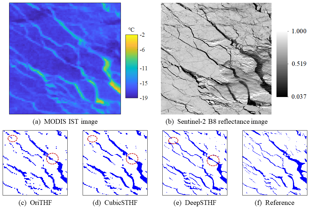
Figure 15(a) The MODIS IST image of a subarea in the Barents Sea; (b) the Sentinel-2 B8 reflectance image; (c) the lead map obtained from the MODIS IST image by the OriTHF method; (d) the lead map obtained from the MODIS IST image by the CubicSTHF method; (e) the lead map obtained from the MODIS IST image by the DeepSTHF method; (f) the reference lead map extracted from the Sentinel-2 image. The red ellipse in panel (e) represents the area impacted by the drifting snow.
The lead mapping results of the OriTHF, CubicSTHF, and DeepSTHF were quantitatively evaluated, and they are given in Table 5. The overall accuracy and MIOU of the DeepSTHF method were larger than those of the OriTHF and CubicSTHF methods, which indicated that the DeepSTHF method achieved the best overall performance among all the methods. The omission errors of the OriTHF and CubicSTHF methods were much larger than that of the DeepSTHF method, indicating that many more lead pixels were not correctly classified, which was consistent with the visual performance. Furthermore, the DeepSTHF had the smallest commission error among all the methods, although it mapped more leads. Consequently, the proposed DeepSTHF method performed well in image SR lead mapping in areas other than the Beaufort Sea.
Table 5The lead mapping results of the OriTHF, CubicSTHF, and DeepSTHF methods.
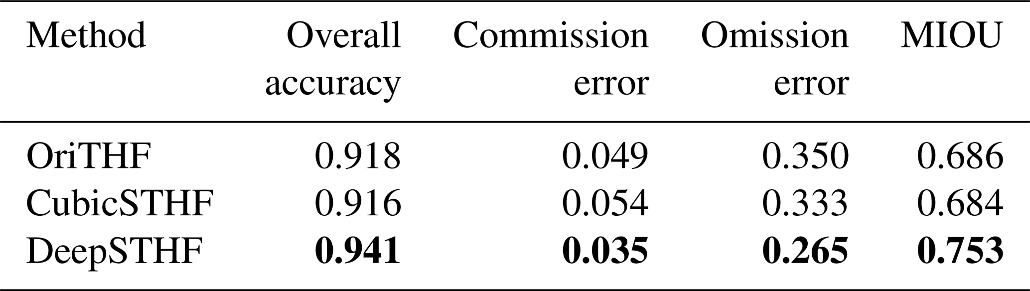
Note that MIOU stands for the mean intersection over union. The most accurate results are highlighted in bold.
5.3 CNN architecture and parameter setting
The enhanced performance of the DeepSTHF method in comparison to the CubicSTHF method is mainly due to the ability of the DeepSTHF to automatically learn the complicated nonlinear relationships between the coarse-resolution IST image and the corresponding fine-resolution IST image and lead map using the two CNN models. In this study, two CNNs with different architectures are used for the IST image SR and SR lead mapping because a single CNN architecture cannot simultaneously achieve different objectives of the two CNN models. The performance of the multi-level feature fusion residual CNN, which was used for lead mapping, was tested on a MODIS SR IST image, and the test results are shown in Fig. 16. Although most fine spatial information has been recovered as red rectangles in Fig. 16b show, the retrieved surface temperature of lead pixels along boundaries was greater than that in the central regions, which caused visual discontinuity, as displayed in the red ellipses in Fig. 16b. This could be because the multi-level feature fusion residual CNN mainly focused on the semantic information of lead networks in the down-sampling layers, which might cause the loss of spatial texture of the input data to a certain extent. Additionally, the very deep CNN used for the SR IST was also proven to be invalid in lead mapping because it could not identify lead networks. A major reason for this was that it did not include any down-sampling layers, and therefore the semantic information of lead networks could be difficult to extract.
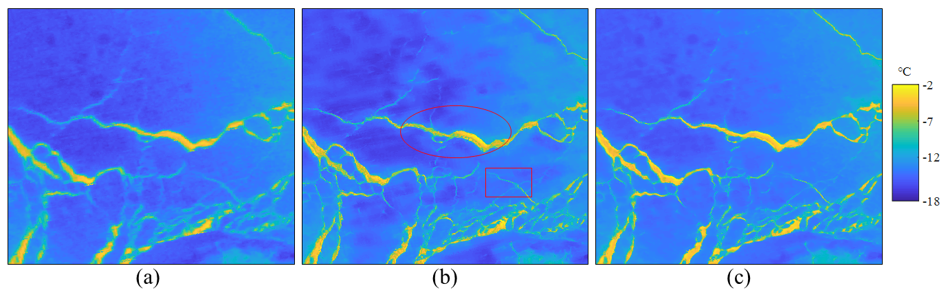
Figure 16Results of the MODIS SR IST imaging for data acquired on 31 March 2020 obtained by (a) the cubic interpolation method, (b) the CNN model with the backbone of the CNN used in SR lead mapping, and (c) the very deep residual CNN model. The red rectangles represent that the fine spatial pattern has been recovered by the multi-level feature fusion residual CNN. The red ellipses represent the recovered surface temperatures of lead pixels by the multi-level feature fusion residual CNN that were not visually continuous.
However, like many classic algorithms, the proposed DeepSTHF method is not totally automatic, and there are certain customized parameters for the CNN models. The batch size of the training samples, an optimization method during the training process, and the learning rate should be set in advance. The optimization method (or optimizer) is a method used in the CNN model training process to adjust the model's weights and biases to minimize the training error. In recent studies, the stochastic gradient descent (SGD) and Adaptive Moment Estimation (Adam) optimizers have been widely used. These two optimizers are the gradient-based methods; their performances regarding the proposed DeepSTHF method were compared, and the results showed that the Adam algorithm could achieve a much faster convergence speed and performed better than the SGD algorithm. As a result, the Adam algorithm was selected as the optimization method in this study. The exponential decay rates β1 and β2 of the Adam algorithm were set to 0.9 and 0.999, respectively, which denoted the values that have been typically recommended in practical applications (Reddi et al., 2019). The learning rate value determines the step size at every iteration while moving toward a minimum of a loss function, and the most appropriate learning rate value for a particular problem mainly depends on the training dataset and model architecture. In this study, the learning rate was set to 10−4, which was empirically found as the most appropriate value for the studied problem. The batch size defines the number of training samples used in one iteration of the model training process. Masters and Luschi (2018) suggested setting the batch size between 2 and 32 because this size can provide the most stable convergence. In this study, the batch size was set to 24, considering the trade-off between the training speed and computational speed of the computer. The experiment showed that the DeepSTHF method could accurately generate subpixel THF data for input data acquired on different dates and covering different areas. However, more suitable model parameter values could be selected in the future, which could provide more accurate results. Determination of the most suitable model parameter values has been a hot topic in the deep learning field, and it requires further investigation.
5.4 Uncertainties and future work
The proposed DeepSTHF method has certain limitations when used in THF estimation. First, there is a large spatial resolution gap between the Landsat-8 and MODIS surface temperature images, which makes the relationship between them complex and difficult to model. Therefore, very narrow lead networks in a fine-resolution image, especially those with a width of less than 5 pixels, cannot be mapped by the proposed DeepSTHF method. In practice, leads can be meters to kilometers wide (Zhang et al., 2018a; Qu et al., 2021), and their widths vary with region and time. For instance, leads are more prevalent in the marginal ice zone comprising much thin ice than in the central Arctic ice pack (Zhang et al., 2018a). Additionally, it has been revealed that lead fractions are minimal in the period from February to early March (in the winter season) when the surface temperature decreases to near its minimum value in a year and then increases quickly in April; the lead fractions then reach more than 10 % ice area in June since the temperature rises largely in the summer season (Qu et al., 2021). Therefore, the reliability of the proposed DeepSTHF decreases as the number of very narrow leads increases, especially in the central Arctic region during the winter season. In addition, in this study, it is assumed that the lead network does not change between the overpass times of the MODIS and Landsat-8 satellites, and the lead maps obtained from the Landsat-8 data are used as reference data in the MODIS imagery experiment, which can introduce certain errors in the training process if an abrupt change occurs in the ice pack. Further, clouds or drifting snow may have a negative impact on the DeepSTHF performance. Namely, the surface temperature of a region contaminated with clouds or drifting snow does not represent reality, so the DeepSTHF parameters obtained in training with the data that contain clouds or drifting snow may not be optimal. In the test process, the clouds or drifting snow outside the lead area will have little impact on the estimated THF over lead, but if they occur in the lead area, the DeepSTHF will not correctly classify the lead pixels and will not accurately reconstruct the corresponding temperature, resulting in an unreliable THF calculation result. Furthermore, since there have been no available meteorological data matching the scale of Landsat imagery, in this study, the meteorological data from the ERA5 dataset are used and interpolated by the cubic interpolation method. Therefore, the potential influence of a warm lead surface on the bottom air might be neglected, which can cause extra uncertainty in the estimated THF.
Although the proposed DeepSTHF achieved the most accurate THF among all the methods in the experiments, there was still a large discrepancy between the estimated and reference THF data, as shown in Fig. 10c. This discrepancy was mainly due to the errors of IST imagery SR reconstruction and SR lead mapping, whose major part originated from the very narrow lead network that the DeepSTHF could not identify, especially those with a width of less than five pixels. Therefore, in practical applications, as the number of very narrow lead networks increases, the uncertainty of the DeepSTHF will increase as well.
The proposed DeepSTHF method can be further improved for future use. First, in this study, the integrated framework is applied with the MODIS thermal images, which have a spatial resolution of 1 km. However, there are other spectral bands with finer resolution in the MODIS product, including the first and second bands with a spatial resolution of 250 m. These finer-resolution images contain more spatial texture than the thermal infrared images, so the accuracy of an SR analysis may be increased by combining them (Li et al., 2013). Second, so as to make sure a lead indicated by the MODIS images is consistent with that of the Landsat-8 images, a change detection method can be first employed to detect abrupt lead change area during the overpass time of the two satellites. Third, the proposed method can achieve higher efficiency for long-term large-area analysis since the fine SST image and lead map can be generated with high efficiency by the proposed CNNs once the model training is completed. Therefore, the proposed method could be applied to produce accurate long-term series THF products using the MODIS images in the Arctic region.
This paper proposes the DeepSTHF method for MODIS thermal infrared imagery. Specifically, the proposed DeepSTHF method includes two CNN models that are used to generate a finer-spatial-resolution IST image and the corresponding finer-resolution lead map from the MODIS IST image. The finer-spatial-resolution data are used for THF estimation. The proposed DeepSTHF method is compared with a pixel-based method, the OriTHF, and a cubic-interpolation-based method, the CubicSTHF, in two experiments using real and simulated data. The results showed that the proposed DeepSTHF acquired more accurate and reliable THF results than the other two methods, which was because it could detect more narrow leads and generate more accurate temperature in the leads area than the OriTHF and CubicSTHF methods. Although DeepSTHF had limitations for very narrow leads and images contaminated by clouds or drifting snow, this study demonstrates the potential of deep learning in the field of THF estimation over leads, where the deep-learning-based methods can represent a favorable tool for analyzing fine variations in leads and the corresponding impact on the climate in the Arctic region.
The source code is available at https://doi.org/10.5281/zenodo.5006637 (Yin and Ling, 2021, last access: 22 June 2021).
The MOD021KM product can be acquired from the US National Aeronautics and Space Administration's Level 1 and Atmosphere Archive and Distribution System Distributed Active Archive Center (https://ladsweb.modaps.eosdis.nasa.gov/, last access: 22 June 2021). The Landsat-8 L1T data can be acquired from the United States Geological Survey Earth Resources Observation and Science Center (http://glovis.usgs.gov/, last access: 22 June 2021). The meteorological data can be acquired from the European Centre for Medium-Range Weather Forecasts (https://cds.climate.copernicus.eu/, last access: 22 June 2021).
FL and ZY designed the proposed method. ZY performed the experiments. ZY wrote the manuscript. YD, YG, FL, and XL revised the manuscript and results. XL and CS provided valuable instructions on data acquisition. All authors read and helped develop the paper.
The authors declare that they have no conflict of interest.
Publisher's note: Copernicus Publications remains neutral with regard to jurisdictional claims in published maps and institutional affiliations.
We sincerely thank the National Aeronautics and Space Administration's Goddard Space Flight Center, the United States Geological Survey, and the European Centre for Medium-Range Weather Forecasts for supplying the datasets used in this study. We also sincerely thank the anonymous reviewers and handling editor Stef Lhermitte for their valuable comments that helped improve our paper.
This research has been supported by the Natural Science Foundation of Hubei Province for Innovation Groups (grant no. 2019CFA019), the National Science Fund for Distinguished Young Scholars (grant no. 41725006), and the National Natural Science Foundation of China (grant nos. 62071457 and 61671425).
This paper was edited by Stef Lhermitte and reviewed by two anonymous referees.
Atkinson, P. M.: Downscaling in remote sensing, Int. J. Appl. Earth Obs., 22, 106–114, https://doi.org/10.1016/j.jag.2012.04.012, 2013.
Aulicino, G., Sansiviero, M., Paul, S., Cesarano, C., Fusco, G., Wadhams, P., and Budillon, G.: A New Approach for Monitoring the Terra Nova Bay Polynya through MODIS Ice Surface Temperature Imagery and Its Validation during 2010 and 2011 Winter Seasons, Remote Sens.-Basel, 10, 366, https://doi.org/10.3390/rs10030366, 2018.
Badrinarayanan, V., Kendall, A., and Cipolla, R.: Segnet: A deep convolutional encoder-decoder architecture for image segmentation, IEEE T. Pattern Anal., 39, 2481–2495, https://doi.org/10.1109/TPAMI.2016.2644615, 2017.
Barber, D. G., Ehn, J. K., Pućko, M., Rysgaard, S., Deming, J. W., Bowman, J. S., Papakyriakou, T., Galley, R. J., and Søgaard, D. H.: Frost flowers on young Arctic sea ice: The climatic, chemical, and microbial significance of an emerging ice type, J. Geophys. Res.-Atmos., 119, 11593–11612, https://doi.org/10.1002/2014jd021736, 2014.
Brodeau, L., Barnier, B., Gulev, S. K., and Woods, C.: Climatologically Significant Effects of Some Approximations in the Bulk Parameterizations of Turbulent Air–Sea Fluxes, J. Phys. Oceanogr., 47, 5–28, https://doi.org/10.1175/jpo-d-16-0169.1, 2017.
Dong, C., Loy, C. C., He, K., and Tang, X.: Image Super-Resolution Using Deep Convolutional Networks, IEEE T. Pattern Anal., 38, 295–307, https://doi.org/10.1109/TPAMI.2015.2439281, 2014.
Du, C., Ren, H., Qin, Q., Meng, J., and Zhao, S.: A Practical Split-Window Algorithm for Estimating Land Surface Temperature from Landsat 8 Data, Remote Sens.-Basel, 7, 647–665, https://doi.org/10.3390/rs70100647, 2015.
Ebert, E. E. and Curry, J. A.: An intermediate one-dimensional thermodynamic sea ice model for investigating ice-atmosphere interactions, J. Geophys. Res.-Oceans, 98, 10085–10109, https://doi.org/10.1029/93jc00656, 1993.
Eppler, D. T. and Full, W. E.: Polynomial trend surface analysis applied to AVHRR images to improve definition of arctic leads, Remote Sens. Environ., 40, 197–218, https://doi.org/10.1016/0034-4257(92)90003-3, 1992.
Eythorsson, D., Gardarsson, S. M., Ahmad, S. K., Hossain, F., and Nijssen, B.: Arctic climate and snow cover trends – Comparing Global Circulation Models with remote sensing observations, Int. J. Appl. Earth Obs., 80, 71–81, https://doi.org/10.1016/j.jag.2019.04.003, 2019.
Fan, P., Pang, X., Zhao, X., Shokr, M., Lei, R., Qu, M., Ji, Q., and Ding, M.: Sea ice surface temperature retrieval from Landsat 8/TIRS: Evaluation of five methods against in situ temperature records and MODIS IST in Arctic region, Remote Sens. Environ., 248, 111975, https://doi.org/10.1016/j.rse.2020.111975, 2020.
Fett, R. W., Englebretson, R. E., and Burk, S. D.: Techniques for analyzing lead condition in visible, infrared and microwave satellite imagery, J. Geophys. Res.-Atmos., 102, 13657–13671, https://doi.org/10.1029/97JD00340, 1997.
Foody, G. M. and Doan, H. T. X.: Variability in Soft Classification Prediction and its implications for Sub-pixel Scale Change Detection and Super Resolution Mapping, Photogramm. Eng. Rem. S., 73, 923–933, https://doi.org/10.14358/PERS.73.8.923, 2007.
Foody, G. M., Muslim, A. M., and Atkinson, P. M.: Super-resolution mapping of the waterline from remotely sensed data, Int. J. Remote Sens. 26, 5381–5392, https://doi.org/10.1080/01431160500213292, 2005.
Ge, Y., Li, S., and Lakhan, V. C.: Development and Testing of a Subpixel Mapping Algorithm, IEEE T. Geosci. Remote, 47, 2155–2164, https://doi.org/10.1109/TGRS.2008.2010863, 2009.
Ge, Y., Jin, Y., Stein, A., Chen, Y., Wang, J., Wang, J., Cheng, Q., Bai, H., Liu, M., and Atkinson, P. M.: Principles and methods of scaling geospatial Earth science data, Earth-Sci. Rev., 197, 102897, https://doi.org/10.1016/j.earscirev.2019.102897, 2019.
Gerace, A. and Montanaro, M.: Derivation and validation of the stray light correction algorithm for the thermal infrared sensor onboard Landsat 8, Remote Sens. Environ., 191, 246–257, https://doi.org/10.1016/j.rse.2017.01.029, 2017.
Glasner, D., Bagon, S., and Irani, M.: Super-resolution from a single image, 2009 IEEE 12th International Conference on Computer Vision, 29 September–2 October 2009, Kyoto, Japan, 349–356, 2009.
Goosse, H., Campin, J.-M., Deleersnijder, E., Fichefet, T., Mathieu, P.-P., Maqueda, M. M., and Tartinville, B.: Description of the CLIO model version 3.0, Institut d'Astronomie et de Géophysique Georges Lemaitre, Catholic University of Louvain, Belgium, 2001.
Hall, D. K., Riggs, G. A., Salomonson, V. V., Barton, J., Casey, K., Chien, J., DiGirolamo, N., Klein, A., Powell, H., and Tait, A.: Algorithm Theoretical Basis Document (ATBD) for the MODIS Snow and Sea Ice-Mapping Algorithms, NASA GSFC: Greenbelt, MD, USA, available at: https://modis-snow-ice.gsfc.nasa.gov/?c=atbd (last access: 22 June 2021), 2001.
Jia, Y., Ge, Y., Chen, Y., Li, S., Heuvelink, G. B. M., and Ling, F.: Super-Resolution Land Cover Mapping Based on the Convolutional Neural Network, Remote Sens.-Basel, 11, 1815, https://doi.org/10.3390/rs11151815, 2019.
Key, J., Maslanik, J., Papakyriakou, T., Serreze, M., and Schweiger, A.: On the validation of satellite-derived sea ice surface temperature, Arctic, 280–287, https://doi.org/10.14430/arctic1298, 1994.
Key, J. R., Collins, J. B., Fowler, C., and Stone, R. S.: High-latitude surface temperature estimates from thermal satellite data, Remote Sens. Environ., 61, 302–309, https://doi.org/10.1016/S0034-4257(97)89497-7, 1997.
Kingma, D. and Ba, J.: Adam: A Method for Stochastic Optimization, arXiv, https://arxiv.org/abs/1412.6980 (last access: 22 June 2021), 2014.
Lanaras, C., Bioucas-Dias, J., Galliani, S., Baltsavias, E., and Schindler, K.: Super-resolution of Sentinel-2 images: Learning a globally applicable deep neural network, ISPRS J. Photogramm. Rem. S., 146, 305–319, https://doi.org/10.1016/j.isprsjprs.2018.09.018, 2018.
Leach, R. and Sherlock, B.: Applications of super-resolution imaging in the field of surface topography measurement, Surface Topography: Metrology and Properties, 2, 023001, https://doi.org/10.1088/2051-672x/2/2/023001, 2013.
Ledig, C., Theis, L., Huszár, F., Caballero, J., Cunningham, A., Acosta, A., Aitken, A., Tejani, A., Totz, J., Wang, Z., and Shi, W.: Photo-Realistic Single Image Super-Resolution Using a Generative Adversarial Network, 2017 IEEE Conference on Computer Vision and Pattern Recognition (CVPR), 21–26 July 2017, Honolulu, HI, USA, 105–114, 2017.
Lewis, B. J. and Hutchings, J. K.: Leads and Associated Sea Ice Drift in the Beaufort Sea in Winter, J. Geophys. Res.-Oceans, 124, 3411–3427, https://doi.org/10.1029/2018jc014898, 2019.
Li, X., Ling, F., Du, Y., and Zhang, Y.: Spatially adaptive superresolution land cover mapping with multispectral and panchromatic images, IEEE T. Geosci. Remote, 52, 2810–2823, https://doi.org/10.1109/TGRS.2013.2266345, 2013.
Lindsay, R. W. and Rothrock, D. A.: Arctic sea ice leads from advanced very high resolution radiometer images, J. Geophys. Res.-Oceans, 100, 4533–4544, https://doi.org/10.1029/94jc02393, 1995.
Ling, F. and Foody, G. M.: Super-resolution land cover mapping by deep learning, Remote Sens. Lett., 10, 598–606, https://doi.org/10.1080/2150704X.2019.1587196, 2019.
Ling, F., Du, Y., Xiao, F., Xue, H., and Wu, S.: Super-resolution land-cover mapping using multiple sub-pixel shifted remotely sensed images, Int. J. Remote S., 31, 5023–5040, https://doi.org/10.1080/01431160903252350, 2010.
Ling, F., Boyd, D., Ge, Y., Foody, G. M., Li, X., Wang, L., Zhang, Y., Shi, L., Shang, C., Li, X., and Du, Y.: Measuring River Wetted Width From Remotely Sensed Imagery at the Subpixel Scale With a Deep Convolutional Neural Network, Water Resour. Res., 55, 5631–5649, https://doi.org/10.1029/2018wr024136, 2019.
Lüpkes, C., Vihma, T., Birnbaum, G., and Wacker, U.: Influence of leads in sea ice on the temperature of the atmospheric boundary layer during polar night, Geophys. Res. Lett., 35, L03805, https://doi.org/10.1029/2007gl032461, 2008.
Marcq, S. and Weiss, J.: Influence of sea ice lead-width distribution on turbulent heat transfer between the ocean and the atmosphere, The Cryosphere, 6, 143–156, https://doi.org/10.5194/tc-6-143-2012, 2012.
Masters, D. and Luschi, C.: Revisiting Small Batch Training for Deep Neural Networks, arXiv, available at: https://arxiv.org/abs/1804.07612 (last access: 22 June 2021), 2018.
Maykut, G. A.: Energy exchange over young sea ice in the central Arctic, J. Geophys. Res.-Oceans, 83, 3646–3658, https://doi.org/10.1029/JC083iC07p03646, 1978.
Montanaro, M., Gerace, A., and Rohrbach, S.: Toward an operational stray light correction for the Landsat 8 Thermal Infrared Sensor, Appl. Optics, 54, 3963–3978, https://doi.org/10.1364/AO.54.003963, 2015.
Noh, H., Hong, S., and Han, B.: Learning Deconvolution Network for Semantic Segmentation, 2015 IEEE International Conference on Computer Vision (ICCV), 7–13 December 2015, Santiago, Chile, 1520–1528, 2015.
Ping, B., Su, F., Han, X., and Meng, Y.: Applications of Deep Learning-Based Super-Resolution for Sea Surface Temperature Reconstruction, IEEE J. Sel. Top. Appl., 14, 887–896, https://doi.org/10.1109/JSTARS.2020.3042242, 2021.
Qu, M., Pang, X., Zhao, X., Zhang, J., Ji, Q., and Fan, P.: Estimation of turbulent heat flux over leads using satellite thermal images, The Cryosphere, 13, 1565–1582, https://doi.org/10.5194/tc-13-1565-2019, 2019.
Qu, M., Pang, X., Zhao, X., Lei, R., Ji, Q., Liu, Y., and Chen, Y.: Spring leads in the Beaufort Sea and its interannual trend using Terra/MODIS thermal imagery, Remote Sens. Environ., 256, 112342, https://doi.org/10.1016/j.rse.2021.112342, 2021.
Reddi, S. J., Kale, S., and Kumar, S.: On the Convergence of Adam and Beyond, arXiv, available at: https://arxiv.org/abs/1904.09237 (last access: 22 June 2021), 2019.
Renfrew, I. A., Moore, G. W. K., Guest, P. S., and Bumke, K.: A Comparison of Surface Layer and Surface Turbulent Flux Observations over the Labrador Sea with ECMWF Analyses and NCEP Reanalyses, J. Phys. Oceanogr., 32, 383–400, https://doi.org/10.1175/1520-0485(2002)032<0383:Acosla>2.0.Co;2, 2002.
Röhrs, J. and Kaleschke, L.: An algorithm to detect sea ice leads by using AMSR-E passive microwave imagery, The Cryosphere, 6, 343–352, https://doi.org/10.5194/tc-6-343-2012, 2012.
Ronneberger, O., Fischer, P., and Brox, T.: U-net: Convolutional networks for biomedical image segmentation, International Conference on Medical image computing and computer-assisted intervention, 5–9 October 2015, Munich, Germany, 234–241, 2015.
Tennekes, H.: The Logarithmic Wind Profile, J. Atmos. Sci., 30, 234–238, https://doi.org/10.1175/1520-0469(1973)030<0234:Tlwp>2.0.Co;2, 1973.
Tschudi, M. A., Curry, J. A., and Maslanik, J. A.: Characterization of springtime leads in the Beaufort/Chukchi Seas from airborne and satellite observations during FIRE/SHEBA, J. Geophys. Res.-Oceans, 107, SHE 9-1–SHE 9-14, https://doi.org/10.1029/2000jc000541, 2002.
Van Doninck, J., Peters, J., De Baets, B., De Clercq, E. M., Ducheyne, E., and Verhoest, N. E. C.: The potential of multitemporal Aqua and Terra MODIS apparent thermal inertia as a soil moisture indicator, Int. J. Appl. Earth Obs., 13, 934–941, https://doi.org/10.1016/j.jag.2011.07.003, 2011.
Wang, Q., Shi, W., and Atkinson, P. M.: Sub-pixel mapping of remote sensing images based on radial basis function interpolation, ISPRS J. Photogramm. Rem. S., 92, 1–15, https://doi.org/10.1016/j.isprsjprs.2014.02.012, 2014.
Wang, Z., Chen, J., and Hoi, S. C. H.: Deep Learning for Image Super-resolution: A Survey, IEEE T. Pattern Anal., 1, 32217470, https://doi.org/10.1109/TPAMI.2020.2982166, 2020.
Willmes, S. and Heinemann, G.: Pan-Arctic lead detection from MODIS thermal infrared imagery, Ann. Glaciol., 56, 29–37, https://doi.org/10.3189/2015AoG69A615, 2015.
Yin, Z. and Ling, F.: Codes of super-resolution of ice surface temperture and super-resolution lead mapping [code], Zenodo, https://doi.org/10.5281/zenodo.5006637, 2021.
Zhang, Y., Cheng, X., Liu, J., and Hui, F.: The potential of sea ice leads as a predictor for summer Arctic sea ice extent, The Cryosphere, 12, 3747–3757, https://doi.org/10.5194/tc-12-3747-2018, 2018a.
Zhang, Y., Tian, Y., Kong, Y., Zhong, B., and Fu, Y.: Residual dense network for image super-resolution, Proceedings of the IEEE conference on computer vision and pattern recognition, 18–23 June 2018, Salt Lake City, UT, USA, 2472–2481, https://doi.org/10.1109/CVPR.2018.00262, 2018b.
Zhong, Y. and Zhang, L.: Sub-pixel mapping based on artificial immune systems for remote sensing imagery, Pattern Recognition, 46, 2902–2926, https://doi.org/10.1016/j.patcog.2013.04.009, 2013.