Implications of surface flooding on airborne estimates of snow depth on sea ice

Snow depth observations from airborne snow radars, such as the NASA's Operation IceBridge (OIB) mission, have recently been used in altimeter-derived sea ice thickness estimates, as well as for model parameterization. A number of validation studies comparing airborne and in situ snow depth measurements have been conducted in the western Arctic Ocean, demonstrating the utility of the airborne data. However, there have been no validation studies in the Atlantic sector of the Arctic. Recent observations in this region suggest a significant and predominant shift towards a snow-ice regime caused by deep snow on thin sea ice. During the Norwegian young sea Ice, Climate and Ecosystems (ICE) expedition (N-ICE2015) in the area north of Svalbard, a validation study was conducted on 19 March 2015. This study collected ground truth data during an OIB overflight. Snow and ice thickness measurements were obtained across a two-dimensional (2-D) 400 m × 60 m grid. Additional snow and ice thickness measurements collected in situ from adjacent ice floes helped to place the measurements obtained at the gridded survey field site into a more regional context. Widespread negative freeboards and flooding of the snowpack were observed during the N-ICE2015 expedition due to the general situation of thick snow on relatively thin sea ice. These conditions caused brine wicking into and saturation of the basal snow layers. This causes the airborne radar signal to undergo more diffuse scattering, resulting in the location of the radar main scattering horizon being detected well above the snow–ice interface. This leads to a subsequent underestimation of snow depth; if only radar-based information is used, the average airborne snow depth was 0.16 m thinner than that measured in situ at the 2-D survey field. Regional data within 10 km of the 2-D survey field suggested however a smaller deviation between average airborne and in situ snow depth, a 0.06 m underestimate in snow depth by the airborne radar, which is close to the resolution limit of the OIB snow radar system. Our results also show a broad snow depth distribution, indicating a large spatial variability in snow across the region. Differences between the airborne snow radar and in situ measurements fell within the standard deviation of the in situ data (0.15–0.18 m). Our results suggest that seawater flooding of the snow–ice interface leads to underestimations of snow depth or overestimations of sea ice freeboard measured from radar altimetry, in turn impacting the accuracy of sea ice thickness estimates.

1 Introduction

Snow and sea ice thickness in a changing Arctic climate system is the matter of many recent studies (e.g., Webster et al., 2018) since the snow layer on top of the frozen ocean generates several contradictory effects on the polar climate. On the one hand, in winter, snow acts as an insulator between the relatively warm ocean and the cold atmosphere and hinders the heat exchange between ocean and atmosphere, reducing the sea ice growth rate (Sturm, 2002; Perovich, 2003). On the other hand, in spring and summer, snow reflects shortwave radiation with its high optical albedo in the range of 0.7–0.85 and prevents the underlying sea ice with an albedo of about 0.6 from melting (Grenfell and Maykut, 1977; Perovich, 1996). In addition, snow cover controls the amount of transmittance of photosynthetically active radiation affecting the productivity of primary algae and phytoplankton (Mundy et al., 2007). Moreover, snow can be a positive contributor to the sea ice mass balance since snow can transform to snow ice (Granskog et al., 2017; Merkouriadi et al., 2017a) and superimposed ice (Eicken et al., 2004; Wang et al., 2015).

Besides the importance of snow from a radiative and mass balance perspective, knowledge of snow depth on sea ice is also required for the accurate retrieval of sea ice thickness from satellite altimetry. The method relies on the assumption that sea ice floating in the ocean is in hydrostatic equilibrium, and sea ice thickness can be calculated by using observations of either ice freeboard (from radar altimeters) or snow freeboard (from laser altimeters) and assumptions about the respective densities of snow, ice and water. Ice and snow freeboards describe the distances above the local sea level to the snow–ice or air–snow interface, respectively. The error budget of the derived ice thickness from laser altimetry is dominated by uncertainties of snow depth and ice and snow densities, as well as uncertainties due to remaining errors in the sea surface height (SSH; Giles et al., 2007; Kern et al., 2015; Skourup et al., 2017).

Thus, accurate knowledge of snow depth on sea ice would be helpful to reduce the error in the sea ice thickness calculations and is important for quantifying climatological processes in polar regions. The Operation IceBridge (OIB) airborne campaigns (Koenig et al., 2010), which began in 2009, measure snow depth and surface elevation with an ultra-wideband snow radar (e.g., Yan et al., 2017) and an airborne topographic mapper (ATM) laser altimetry system (Krabill et al., 2002), respectively. With these sensors, both the air–snow and the snow–ice interfaces can be detected with the snow radar (e.g., Newman et al., 2014), and the surface elevation can be mapped with the ATM (e.g., Farrell et al., 2012). Hence, the OIB data are a valuable source for validating satellite remote sensing sea ice products, as well as for model parameterization. Furthermore, the comparison of airborne OIB data with in situ field measurements is necessary to understand the processes affecting radar penetration into snow-covered sea ice and the impact of the snow load on the snow–ice interface.

Several OIB validation studies have been conducted (e.g., Farrell et al., 2012; Webster et al., 2014; Newman et al., 2014; Holt et al., 2015), and multiple snow depth retrieval algorithms were developed (e.g., Kurtz et al., 2013, 2014; Newman et al., 2014; Kwok and Maksym, 2014) and compared with satellite products (Kwok et al., 2017; Lawrence et al., 2018). These studies have provided insights about the snow depth uncertainty and the errors associated with the airborne techniques (Kwok, 2014; King et al., 2015). However, in the Northern Hemisphere, all evaluation studies (except those connected to satellite data) have thus far focused on snow in the Canada Basin, in the central Arctic Ocean or only in peripheral subregions of the Arctic. To our knowledge, no OIB validation study has been conducted in the Atlantic sector of the Arctic.

In recent years, a significant change towards thinner ice with thicker snow cover (Renner et al., 2014; Rösel et al., 2018) has been observed in this region, caused by an increase in intense storm events and associated precipitation in this area (Woods and Caballero, 2016; Graham et al., 2017; Rinke et al., 2017). In addition, previous studies indicate that radar signal penetration through the snow pack might be lower under certain geophysical snow-ice conditions in this area (Gerland et al., 2013; King et al., 2018; Nandan et al., 2020) and also in the Antarctic (Kwok and Kacimi, 2018; Willatt et al., 2010). Snow and ice conditions in this region differ to those in the Canada Basin and central Arctic (e.g., Webster et al., 2014, 2018), and they have been found to induce substantial negative ice freeboards with subsequent flooding of the snow pack more akin to the conditions in the seasonal ice pack of the Southern Ocean (Massom et al., 2001). This may have an impact on remote sensing methods of snow and ice thickness estimation, which have so far only been validated for more typical Arctic conditions.

In this paper, we present in situ observations of sea ice and snow depth and snow and ice characteristics from the N-ICE2015 expedition, alongside near-coincident airborne measurements acquired on 19 March 2015 during an OIB overflight. We calculate ice freeboard values from a variety of sensors to investigate the prevalence of negative freeboards and flooding at the snow–ice interface. We investigate the impact of flooded snow layers on the airborne radar observations. Utilizing a combination of methodologies, we assess sea ice thickness conditions in the region. We discuss our results in the context of satellite-derived ice thickness and consider the impact of flooding on estimating thickness in regions with thin sea ice and deep snow, such as in the Atlantic section of the Arctic Ocean or in the Southern Ocean.

2 Data and methods

2.1 Study area

Field observations for this study were acquired during the Norwegian young sea Ice, Climate and Ecosystems (ICE) expedition (N-ICE2015) with R/V Lance. The expedition started in the Arctic Ocean north of Svalbard at 83^∘15^′ N, 21^∘32^′ E on 15 January 2015 and concluded at 80^∘ N and 5^∘36^′ E on 22 June 2015 and consisted of a series of four drift segments (Granskog et al., 2016, 2018). In this study, we focus on sea-ice- and snow-related observations from the drift of Floe 2, covering a time period from 24 February to 19 March 2015. Data from the OIB overflight employed in this study were collected on 19 March 2015 at 82^∘29^′ N and 22^∘37^′ E above the drifting sea ice floe.

The ice station on Floe 2 was set up on an aggregation of different ice types: refrozen leads, first-year ice (FYI) and second-year ice (SYI). Modal sea ice thickness at the field station was 0.3, 0.9 and 1.7 m for refrozen leads, FYI and SYI, respectively (Rösel et al., 2017). Snow depth was on average 0.56 ± 0.17 m on FYI and SYI (Rösel et al., 2017), while on refrozen leads it was approximately 0.02 m, likely redistributed from blowing snow. For this study, a 400 m × 60 m survey field was established. Red flag poles, with black snow-filled trash bags, marked the outline making it visible from air (see Fig. 1). Shortly after OIB overflights, snow depth and sea ice thickness observations were collected on this two-dimensional (2-D) survey field using a “snake line” sampling pattern with 5 m spacing between lines across the short axis of the field (see Fig. 1).

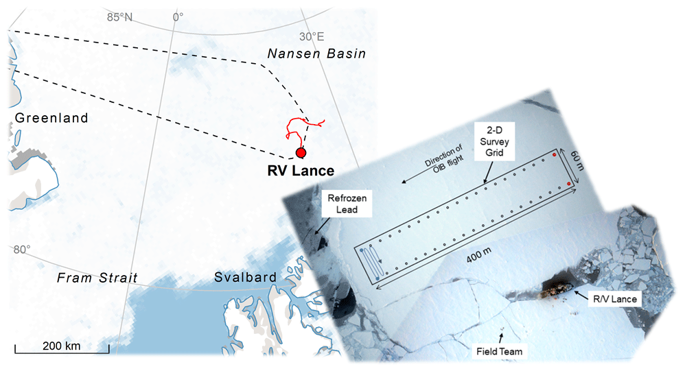
Figure 1 Overview of the location in the Arctic Ocean (left) and setup of the 2-D in situ survey field situated on an ice floe as a part of the Floe 2 drifting phase to the west of R/V Lance on 19 March 2015 (right). Digital mapping system (DMS) imagery (Dominguez, 2010, updated 2018) acquired during the OIB overflights was mosaicked to produce the aerial overview map. Black dots indicate the outline of the 2-D survey field. Snow and ice thickness measurements were obtained along the snake-line sampling pattern, as indicated in the left of the survey field.

2.2 Ground-based measurements

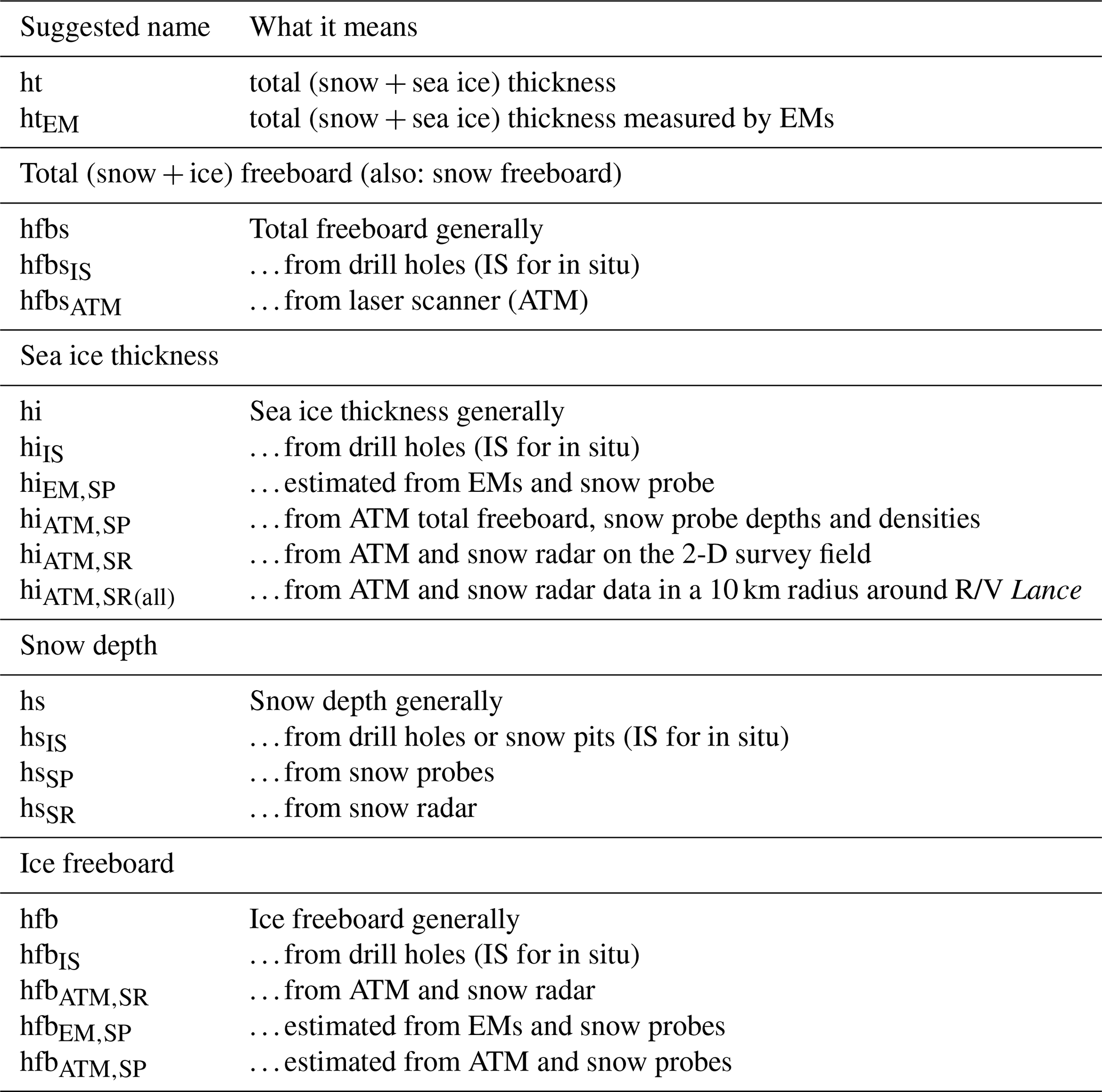
Snow depth measurements (hs_SP, N=1046; variable abbreviations are defined in Table 1) were obtained with a GPS snow probe (SP) from Snow-Hydro (Fairbanks, AK, USA). The snow probe is a thin pole with a sliding disk 0.2 m in diameter. The pole penetrates the snow pack to the snow–sea-ice interface, while the disk rests on the snow surface. Inside the pole a magnetic device measures the distance between the disk and the lower tip of the pole providing the snow depth (Sturm and Holmgren, 1999, 2018). Each measurement is time-tagged and geolocated and is recorded on a data logger. The accuracy of the measurements over sea ice may vary between ± 1–3 mm (Marshall et al., 2006; Sturm and Holmgren, 2018), and the footprint is the size of the disk (i.e., 0.2 m). Snow depth measurements were made approximately every 5 m following the snake line sampling pattern within the 2-D survey field (see Fig. 1).

Total snow and ice thickness measurements (h_t; N=7005) were obtained using the EM31 electromagnetic device (Geonics Ltd., Mississauga, Ontario, Canada). A person dragging the EM31 instrument on a plastic sledge followed the snow probe sampler. The EM31 measurements were sampled with a frequency of 2 Hz. The footprint size of the EM31 ranges from 3 to 5 m (e.g., Haas et al., 1997) depending on the ice and snow depth. The accuracy of the EM31 measurements is approximately ±0.1 m for level ice and decreasing over deformed ice (Haas et al., 2009).

For comparison to the EM31 data and to collect direct measurements, we drilled 10 equally spaced holes around the 2-D field perimeter with a 2 in (5.08 cm) auger to measure ice thickness, snow depth and ice freeboard. Ice thickness observations were made with a thickness gauge from Kovacs Enterprises (Roseburg, OR, USA). The gauge is a specific tape measure with a foldable metal weight at the bottom that can be deployed through the drill holes. The accuracy of the readings is estimated to be ±0.01 m. In addition, a snow pit was dug in the vicinity of the 2-D survey field (Merkouriadi et al., 2017c) to assess snow structure, and an ice core was obtained to measure ice salinity, temperature and density (Gerland et al., 2017). The core was extracted with a 0.09 m diameter ice corer from Kovacs Enterprises (Roseburg, OR, USA).

To provide a regional context for the observations made in the 2-D field, we use a set of long, and independent, transects with combined EM31 and snow depth measurements (N=5060) obtained within a maximum radius of 5 km around the ship during the N-ICE2015 expedition. These were performed to characterize the spatial variability in snow and ice thickness in the area surrounding the main ice camp. Further details can be found in Rösel et al. (2018). We use the 2-D grid snow depth measurements and those sampled via transects within a 5 km radius to provide spatial representativeness and context from local to regional scales.

2.3 Airborne measurements

The OIB aircraft surveyed the 2-D survey field three times (see Fig. 2) on 19 March 2015. First a surveillance overflight occurred at 15:28 UTC. A second and third pass directly over the 2-D survey field occurred at 15:37 and 15:43 UTC, respectively. Because the first pass did not adequately intersect the 2-D survey field, we focus our analysis on measurements obtained during passes 2 and 3 of the aircraft. Although the ice floe drifted during the airborne survey, the alignment of transects 2 and 3 were such that they directly intersected the 2-D survey field on both passes.

For sea ice studies, the aircraft was equipped with an ATM laser altimeter system (Krabill et al., 2002), an ultra-wideband frequency-modulated continuous waveform (FMCW) snow radar system (e.g., Yan et al., 2017) and a digital mapping system (DMS) that provides high-resolution (0.1 m) geolocated visible-band images of the snow surface (Dominguez, 2010, updated 2018) allowing for visual interpretation of sea ice conditions in the vicinity of the 2-D survey field (see Fig. 1).

Figure 2 Detailed airborne mapping of the snow freeboard (5 m grid, derived from ATM observations of surface elevation) and snow depth (superimposed dots, derived from the airborne snow radar) at the 2-D survey field (corner points indicated by black stars) located on Floe 2. The three airborne transects across the field are indicated. During the OIB survey, the ice floe drifted south at an approximate drift speed of 0.15 m s⁻¹. Wavelet (WAV) snow depth on the secondary y axis refers to the snow depth retrieved using the NOAA wavelet technique (Newman et al., 2014).

2.4 Methodology

2.4.1 Drift correction

To obtain spatial coincidence between the in situ and airborne measurements of snow depth, freeboard and sea ice thickness, the positions of all measurements were corrected to mitigate the impact of the drifting sea ice during the experiment. As a reference, we determined the position of the four corners of the 2-D survey field using the DMS imagery collected during the second and third OIB overpasses. By comparing the differences for each corner marker between the two overpasses, we were able to deduce that the ice floe was drifting south at a speed of 0.15 m s⁻¹. To correct for the drift that occurred during the EM31 and SP sampling of the 2-D survey field, we followed the procedure described in Rösel et al. (2018): the EM31 data were resampled onto the coordinates of the SP track, and a Gaussian filter was applied to the EM31 data. Afterwards, both the EM31 and the SP data were interpolated on a 5 m regular grid.

Table 1 A summary of all the variables used in the following context.

2.4.2 Density of seawater, ice and snow

In all calculations we used the following values: the density for seawater was ρ_W=1027 kg m⁻³ (Meyer et al., 2017), the bulk density for the snow pack was ρ_s=328 kg m⁻³ (Merkouriadi et al., 2017b), and the bulk density for sea ice was ρ_i=910 kg m⁻³ (Gerland et al., 2017). All values are based on measurements obtained during the N-ICE2015 expedition at Floe 2.

2.4.3 In situ snow depth sea ice thickness and freeboards

In Fig. 3, the concept of isostatic equilibrium is shown for four cases: on the left side, the ratio of snow depth (hs) to sea ice thickness (hi) is smaller, resulting in a positive sea ice freeboard (hfb) or ice freeboard at sea level. On the right side, the situation of the “new” Arctic as described in Rösel et al. (2018) is schematically presented: a thick snow layer hs is pushing a relatively thin sea ice hi layer below the ocean surface. The resulting sea ice freeboard hfb becomes negative, and subsequently the sea ice surface is vulnerable to flooding.

To obtain sea ice thickness (hi_EM,SP) from SP and EM31 measurements, the resampled snow depth measurements from SP (hs_SP, N=1046) were subtracted from the total sea ice thickness from EM31 measurements (ht_EM, N=1046):

$$\begin{array}{}\text{(1)}& {\mathrm{hi}}_{\mathrm{EM},\mathrm{SP}}={\mathrm{ht}}_{\mathrm{EM}}-{\mathrm{hs}}_{\mathrm{SP}}.\end{array}$$

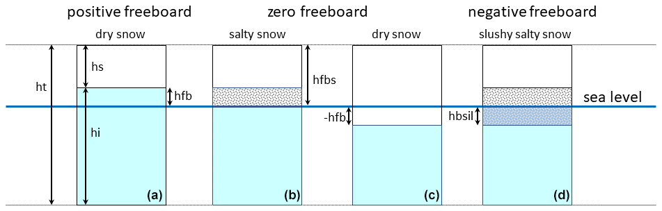
Figure 3 Some examples to show the concept of isostatic equilibrium of sea ice. In (a), the ratio of snow depth (hs) to sea ice thickness (hi) is small, and sea ice freeboard (hfb) is positive. In (c) and (d), the ratio of hs to hi is high, and hfb is negative. In (b), while the sea ice freeboard (hfb) is zero, the lower part of the snow pack can be salty from brine wicking. This can also occur for positive ice freeboards. Panel (d) shows a slushy salty snow layer (hfbsil) due to surface flooding, whereas panel (c) has a dry, non-salty snow cover. The snow freeboard hfbs is the same in all four cases.

Assuming an isostatic equilibrium assumption, hi_EM,SP under dry snow conditions can be calculated as follows:

$$\begin{array}{}\text{(2)}& {\mathrm{hi}}_{\mathrm{EM},\mathrm{SP}}={\mathrm{hfbs}}_{\mathrm{EM},\mathrm{SP}}\left({\displaystyle \frac{{\mathit{\rho }}_{\mathrm{W}}}{{\mathit{\rho }}_{\mathrm{W}}-{\mathit{\rho }}_{\mathrm{i}}}}\right)-\left({\displaystyle \frac{{\mathit{\rho }}_{\mathrm{W}}-{\mathit{\rho }}_{\mathrm{s}}}{{\mathit{\rho }}_{\mathrm{W}}-{\mathit{\rho }}_{\mathrm{i}}}}\right){\mathrm{hs}}_{\mathrm{SP}},\end{array}$$

which results in the freeboard (hfbs_EM,SP) derived from the snow probe (SP) and electromagnetic measurements (EMs) using the obtained snow depth and sea ice thickness information and densities given above:

$$\begin{array}{}\text{(3)}& {\mathrm{hfbs}}_{\mathrm{EM},\mathrm{SP}}={\displaystyle \frac{{\mathrm{hi}}_{\mathrm{EM},\mathrm{SP}}\left({\mathit{\rho }}_{\mathrm{W}}-{\mathit{\rho }}_{\mathrm{i}}\right)+({\mathit{\rho }}_{\mathrm{W}}-{\mathit{\rho }}_{\mathrm{s}}){\mathrm{hs}}_{\mathrm{SP}}}{{\mathit{\rho }}_{\mathrm{W}}}}.\end{array}$$

For wet snow conditions, or a flooded state of the sea ice, we refer to the studies of Zwally et al. (2008) and Ozsoy-Cicek et al. (2013), in which either hs is set equal to hfbs or a slush layer is included in the calculations, respectively. In addition, we gain in situ information from the drill-hole readings: sea ice thickness (hi), snow depth (hs), freeboard (hfb) and snow freeboard (hfbs).

$$\begin{array}{}\text{(4)}& \mathrm{hfbs}=\mathrm{hfb}+\mathrm{hs}\end{array}$$

As described in Rösel et al. (2018), the uncertainty of the ice freeboard hfb_EM,SP and the total freeboard hfbs resulting from the propagation of uncertainties in the snow and ice densities and the sampling uncertainty is estimated to be on average ±0.06 m. The accuracy of freeboard hfb_IS and hfbs_IS from the in situ drill-hole measurements is ±0.01 m (Rösel et al., 2018).

2.4.4 Airborne snow depth, sea ice thickness and freeboards

The DMS images were used to identify the geographical coordinates of areas of open water (with little or no ice cover) within the large refrozen lead, located in the southwest of the 2-D survey field site and adjacent to it (see Fig. 1). ATM elevation measurements associated with these areas were averaged to estimate the local sea surface height (SSH). The SSH within the lead was then subtracted from all ATM elevations to obtain the ATM snow freeboard (hfbs_ATM). Individual ATM measurements were resampled on the same 5 m regular grid as the in situ snow and ice measurements across the sea ice floe (see Fig. 2). The snow radar echoes from passes 2 and 3 from the OIB survey also illustrate the presence of open water, refrozen leads and areas with deep snow cover on the N-ICE2015 ice floe (see Fig. 4).

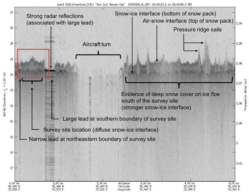
Figure 4 Processed and annotated OIB snow radar echoes surveyed from the 2-D survey field during the third pass on 19 March 2015 at 15:43 UTC. The red bounding box indicates the close-up of the region as shown in Figs. 1 and 2.

We calculated snow depth from snow radar (hs_SR) following the methodology of Newman et al. (2014). Since the basal snow layers were saline in some locations, the snow–ice interface could not always be detected. Therefore, a running average at 25 m length scale (equivalent to five snow radar measurements) was used to account for an observed diffuse snow–ice interface at the 2-D survey field site, possibly caused by a saline basal layer in the lower snow pack.

Ice freeboard (hfb_ATM,SP) and sea ice thickness (hi_ATM,SP), including a potentially refrozen slush layer, can be derived from a combination of the airborne data measurements acquired over the 2-D survey field site with the in situ snow-probe data and were calculated as follows:

$$\begin{array}{}\text{(5)}& {\displaystyle }{\mathrm{hfb}}_{\mathrm{ATM},\mathrm{SP}}={\mathrm{hfbs}}_{\mathrm{ATM}}-{\mathrm{hs}}_{\mathrm{SP}},\text{(6)}& {\displaystyle }{\mathrm{hi}}_{\mathrm{ATM},\mathrm{SP}}={\displaystyle \frac{{\mathit{\rho }}_{\mathrm{W}}{\mathrm{hfb}}_{\mathrm{ATM},\mathrm{SP}}}{{\mathit{\rho }}_{\mathrm{W}}-{\mathit{\rho }}_{\mathrm{i}}}}+{\displaystyle \frac{{\mathit{\rho }}_{\mathrm{s}}{\mathrm{hs}}_{\mathrm{SP}}}{{\mathit{\rho }}_{\mathrm{W}}-{\mathit{\rho }}_{\mathrm{i}}}}.\end{array}$$

In addition, ice freeboard can be calculated through the difference between the ATM snow freeboard (hfbs_ATM) and the snow radar snow depth (hs_SR); hfb_ATM,SR is effectively the freeboard of a radar reflecting layer, including the ice freeboard plus a frozen snow-ice basal layer, if present.

$$\begin{array}{}\text{(7)}& {\mathrm{hfb}}_{\mathrm{ATM},\mathrm{SR}}=\mathrm{hfb}+\mathrm{hbsil}+E={\mathrm{hfbs}}_{\mathrm{ATM}}-{\mathrm{hs}}_{\mathrm{SR}},\end{array}$$

where hfb is the ice freeboard, hbsil is the thickness of the slushy snow-ice basal layer, and E is any remaining errors due to the interface-picking algorithms as applied to the snow radar echoes (Fig. 4).

3 Results

3.1 In situ and airborne measurements from the 2-D survey field site and their comparison

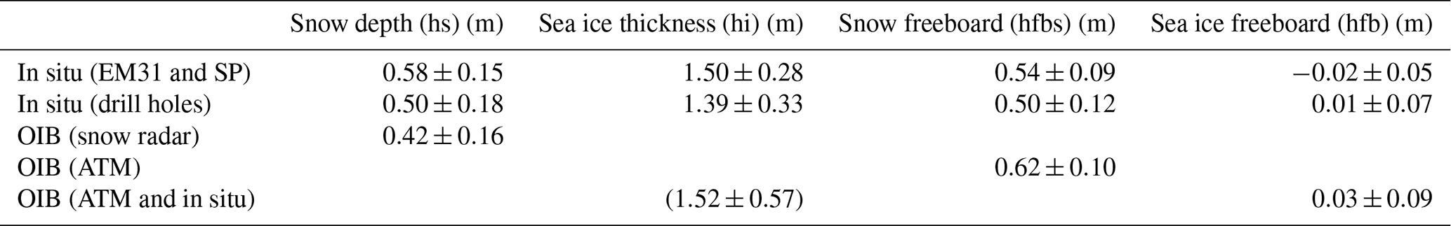
The average calculated sea ice thicknesses (hi_IS; Eq. 1) at the 2-D survey field site is 1.50±0.28 m with a mode of 1.40 m, and the average snow depth measured with the snow probe is ${\mathrm{hs}}_{\mathrm{SP}}=\mathrm{0.58}\pm \mathrm{0.15}$ m with a mode of 0.55 m (results summarized in Table 2). The drill-hole measurements lie within the standard deviation of all measurements collected at the 2-D survey field site; i.e., our results demonstrate very good agreement across all observation methods (Fig. 5 and Table S1 in Supplement). A total of 3 out of the 10 drill holes were found to be flooded.

Table 2 Results of snow, sea ice and freeboard measurements and calculations of the 2-D survey field site.

For direct comparison of the in situ sampled snow depth and ice thickness data, a subset of the snow radar data of both overpasses over the 2-D survey field site, limited by the four corner coordinates of the 2-D survey field (N=62), results in an average snow depth of ${\mathrm{hs}}_{\mathrm{SR}}=\mathrm{0.42}\pm \mathrm{0.16}$ m, with a mode of 0.40, which is 0.16 and 0.15 m lower than the mean and modal snow depth measured in situ at the 2-D survey field site, respectively (N=1046; Fig. 5a). However, the standard deviations, i.e. the width and shape of the snow depth distributions, for both the in situ and airborne snow radar observations are in very good agreement with values of 0.15 and 0.16 m, respectively. In addition, the average snow depth from the airborne snow radar was 0.08 m smaller than average snow depth at the drill-hole locations: ${\mathrm{hs}}_{\mathrm{IS}}=\mathrm{0.50}\pm \mathrm{0.18}$ m (N=10; Fig. 5a).

Figure 5 Probability density functions of snow depth measurements with given average values (μ), standard deviations (σ) and number of measurements (N) from (a) the 2-D survey field site obtained with the snow probe (grey dashes), the OIB snow radar (blue dots) and drill holes (light blue bars) and (b) from the wider surroundings from snow probe sampling during the entire N-ICE2015–Floe 2 campaign (grey dashes) and from OIB snow radar within a radius of 10 km around the position of R/V Lance (blue dots).

3.2 Local- vs. regional-scale snow depth and sea ice thickness measurements

During the N-ICE2015 expedition, long transects on different predefined lines with combined EM31 and snow depth measurements were performed to examine the spatial variability of the area surrounding the main ice camp and included measurements of thin ice and deformed ice areas (Rösel et al., 2018). Altogether, five transects with 5060 gridded snow and ice measurements were made on Floe 2, covering a time period from 24 February to 19 March 2015, which resulted in an average snow depth of 0.55±0.18 m and an average sea ice thickness of 1.09±0.92 m. As stated in Rösel et al. (2018), the snow and ice conditions were on average stable and did not change during the time of the drift.

As shown in Rösel et al. (2017), the overall measurements on the local area scale are representative of sea ice in the region. To gain knowledge about the agreement in the snow depth between the airborne and in situ observations on a more regional scale, we compared observations from the OIB snow radar measurements from the same flight within a 10 km radius around the position of R/V Lance with the average in situ snow depth transect measurements during the drift of Floe 2. Similar to the results obtained at the 2-D survey field site, the snow distributions show an offset for the airborne snow radar data towards lower snow depth values. The average snow depth from the airborne snow radar was 0.49±0.25 m, 0.06 m below the average snow depth of 0.55±0.18 m measured directly with the SP (Fig. 5b). While the one-to-one comparison over the survey field can be considered as a direct validation study, the statistical regional comparison across the larger area can potentially be influenced by geophysical and thermodynamic processes, such as ice dynamics, snow redistribution, snow metamorphism, etc., that occurred during the entire drift duration of Floe 2 (23 d) for which in situ data were acquired.

For comparison with the ice freeboard, ${\mathrm{hfb}}_{\mathrm{IS}}=\mathrm{0.01}\pm \mathrm{0.07}$ m, observed at the drill-hole sites, we used the in situ ground measurements, i.e., SP and EM31, to derive a freeboard of ${\mathrm{hfb}}_{\mathrm{EM},\mathrm{SP}}=-\mathrm{0.02}\pm \mathrm{0.05}$ m with an uncertainty of ±0.06 m (Rösel et al., 2018), following Eq. (3).

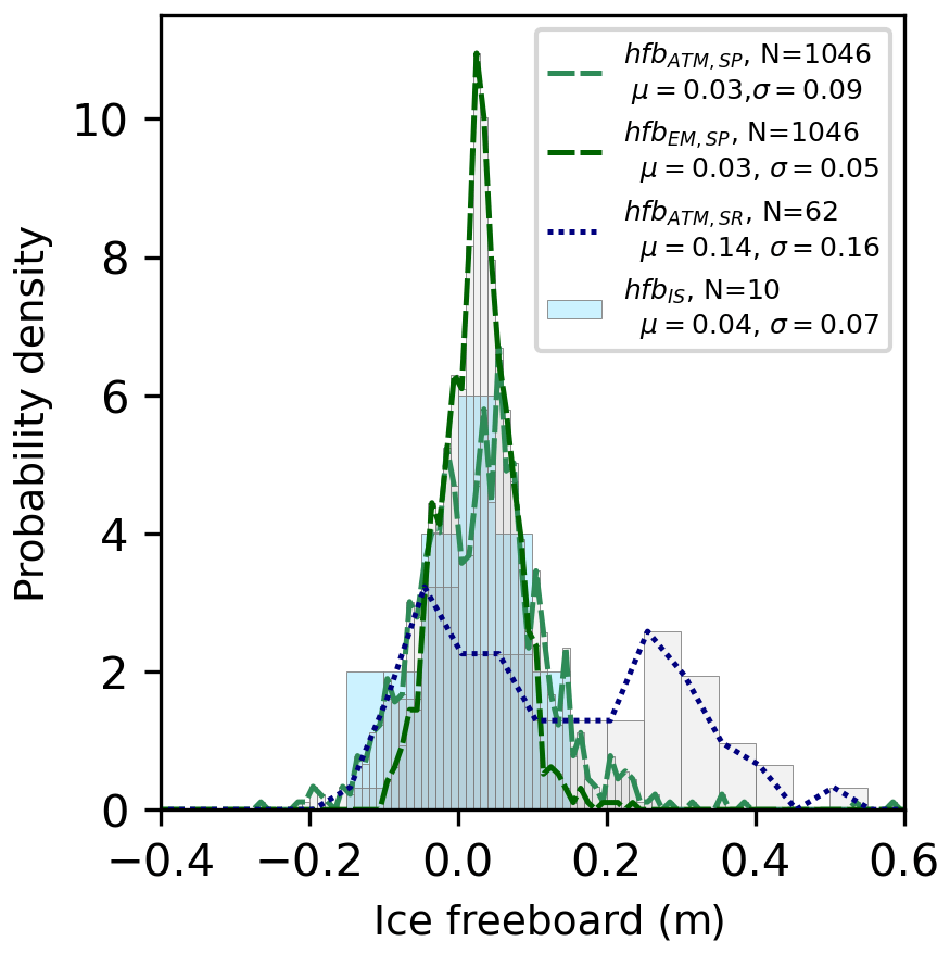
Figure 6 Probability density functions (PDFs) of ice freeboard (hi) with given average values (μ), standard deviations (σ) and number of measurements (N) from the 2-D survey field site: hfb_ATM,SP (light green dashes): freeboard calculated from SP snow depth and ATM surface elevations using Eq. (2); hfb_EM,SP (dark green dashes): ice freeboard from EMs and SP measurements; hfb_ATM,SR (dark blue dots): ice freeboard derived from ATM surface elevation minus matched SR snow depths within the 2-D field; hfb_IS (light blue bars): ice freeboard from drill-hole observations on 2-D field edges, plotted as a regular histogram for tidy visualization.

While the average freeboard at the 2-D survey field site is close to 0 m based on the drill-hole measurements alone, the distribution of freeboards shown in Fig. 6 are negative with magnitudes up to 0.1 m. Results in the same range are obtained by subtracting the snow probe measurements from ATM surface elevation, resulting in an average value of ${\mathrm{hfb}}_{\mathrm{ATM},\mathrm{SP}}=\mathrm{0.03}\pm \mathrm{0.09}$ m (see Fig. 6). Taking the ±0.06 m uncertainty into account, this results in a negative freeboard area fraction of 19 % and 14 % across the 2-D survey field site for hfb_EM,SP and hfb_ATM,SP, respectively (see Fig. 7). An estimate of the ice freeboard plus the thickness of the snow-ice basal layer at the survey site that was impacted by brine wicking may be obtained by subtracting the snow radar measurements from the nearest ATM surface elevation value, which results in an average of ${\mathrm{hfb}}_{\mathrm{ATM},\mathrm{SR}}=\mathrm{0.20}\pm \mathrm{0.10}$ m but that varies across the site (Fig. 7c). The subsequent difference between hfb_ATM,SR and hfb_ATM,SP provides an approximate estimate of the thickness of the flooded, slushy, snow-ice basal layer of the snow cover.

Figure 7 Ice freeboards (hfb) over the survey site: (a) hfb_EM,SP computed using Eq. (3) with EM and snow probe data gridded at 5 m; (b) hfb_ATM,SP using ATM surface elevation and SP snow depths gridded at 5 m. (c) The difference between hfb_EM,SP and hfb_ATM,SP.

Finally, in Fig. 8, we show the sea ice thickness distributions collected at the 2-D survey field site hi_EM,SP and hi_IS, as well as for the region surrounding R/V Lance, hi_ATM,SR(all). For comparison we include hi_ATM,SP calculated from a combination of the ATM data and the in situ snow probe measurements. The in situ measurements show that the 2-D survey field site was situated on an ice floe ranging between 1.4 and 1.5 m thick (Fig. 8). This compares to a thinner regional-scale ice cover (1.09±0.92 m), as measured from Floe 2. The variability in sea ice thickness in the region surrounding R/V Lance is about 3 times larger than that at the 2-D survey field site. This is to be explained with a higher variability of ice types that were covered during the regular transects on Floe 2, including thin ice areas as well. We note that the average sea ice thickness of the 2-D survey site, hi${}_{\mathrm{ATM},\mathrm{SP}}=\mathrm{1.52}$ m, is only slightly above hi${}_{\mathrm{EM},\mathrm{SP}}=\mathrm{1.50}$ m, although the thickness equation (Eq. 6) does not take into account the two-layer snow setup, with each snow layer having a different depth and density. This is consistent with the result shown in Fig. 6, which presents the same freeboards for hfb_EM,SP and hfb_ATM,SP. Comparing the distributions of hfb_ATM,SP and hfb_EM,SP with hfb_ATM,SR (Fig. 6), hfb_ATM,SR has a clear bimodal distribution with the first mode at −0.05 m, which indicates the main scattering horizon of the snow radar, and the second mode at 0.25 m. This high second mode is potentially caused by wet or saline snow pushing the main reflecting horizon for the snow radar upwards, as will be discussed below.

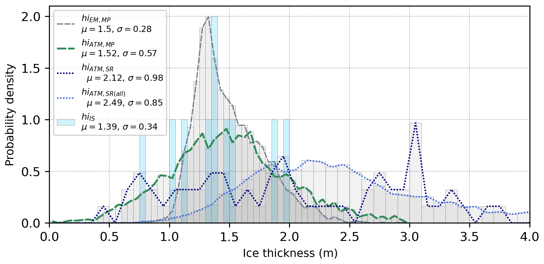
Figure 8 PDFs of sea ice thickness (hi) with given average values (μ), standard deviations (σ) and number of measurements (N) from the 2-D survey field site: hi_EM,SP (dashed grey): ice thickness calculated from EM31 total thickness and SP snow depth; hi_ATM,SP (dashed green): ice thick calculated from ATM surface elevation and SP snow depth in the 2-D field; hi_ATM,SR (dark blue dots): ice thickness calculated from ATM surface elevation and snow radar data using matched OIB ATM and radar observations in the 2-D field; hi_ATM,SR(all) (blue dots): ice thickness from all ATM surface elevation measurements in a 10 km radius around R/V Lance and the mean of all radar snow depth estimates; hi_IS (light blue bars): ice thickness measured in situ at drilling sites around the survey plot.

4 Discussion and conclusions

The mean and modal snow depth estimates derived from the snow radar were 0.12 m lower than the in situ snow probe measurements obtained at the 2-D survey field site. Over a larger regional scale of 10 km radius from the R/V Lance location, snow depth estimates derived from the snow radar underestimate in situ snow-probe-derived snow depth by 0.06 m, which is close to the measurement uncertainty of the snow radar system associated with its range resolution (Newman et al., 2014).

In radar altimetry, it is assumed that the radar signal penetrates completely through a dry snow pack and energy is reflected from the snow–ice interface, which represents the height of the sea ice freeboard above local sea level. This assumption is valid (Beaven et al., 1995) for a cold, dry and homogenous snow pack, typical of Arctic sea ice in winter. However, for snow packs exhibiting high moisture content or higher densities (e.g., due to ice lenses and/or crusts), radar signals undergo absorption within the snow volume (e.g., Kwok and Maksym, 2014; Ricker et al., 2015). Recent studies suggest reduced signal penetration into the snow pack with a more diffuse snow–ice interface on both Arctic and Antarctic sea ice (Willatt et al., 2010, 2011, Gerland et al., 2013; Kwok and Kacimi, 2018), especially if the snow pack is saline (Nandan et al., 2020, 2017) or very deep with ice lenses present (King et al., 2018). In addition, deep snow pushes the ice surface below the water level, leading to negative freeboard that might induce flooding and the formation of highly saline slush layers in the basal layers of the snow pack, which, when measured with a radar altimeter system, can result in a dominant scattering horizon above the true snow–ice interface (Nandan et al., 2020) and hence an overestimation of ice freeboard and thus sea ice thickness and an underestimation of snow depth (Figs. 6 and 8).

On FYI, overlying snow also wicks brine upwards from the sea ice surface during freeze-up, producing saline snow layers predominately observed in the bottommost 0.06–0.08 m of the snow pack (Drinkwater and Crocker, 1988; Geldsetzer et al., 2009; Nandan et al., 2016, 2017, 2020). The salinity profile of the ice core, taken on 5 March 2015 in the vicinity of the 2-D survey field site, shows a typical C-shape profile with relatively high salinity values of up to 11.3 psu at the top and 5.8 psu at the bottom and lower values of between 1.3 and 4.3 psu in the middle sections of the ice core (see Fig. 9), suggesting that the 2-D survey field site on the ice floe was comprised of FYI. Snow salinity observations from snow covers (0.26 and 0.34 m thick) overlying the FYI floe indicate highly saline, 0.10 m deep basal layers in both snow covers by up to 10 psu. Additionally, one-third of the drill holes at the 2-D field site indicated flooding of the snow pack and negative freeboard, which induced the formation of highly saline and saturated slush in the basal snow layers. The presence of slush layers at the 2-D field site resulted in a challenging geophysical setting for the measurement of snow and ice thickness using remote sensing techniques, which involve snow radar measurements.

Figure 9 Salinity profile and auxiliary data of an ice core taken on 5 March 2015 within the vicinity of the 2-D survey field.

Previous studies (Barber et al., 1998; Barber and Nghiem, 1999; Nghiem et al., 1995; Geldsetzer et al., 2009; Nandan et al., 2017, 2020) have reported the impact of saline snow on FYI which alters the geophysical, thermodynamic, dielectric and radar scattering properties of the snow cover, thereby impacting radar signal penetration through the snow pack. Nandan et al. (2017) showed that a saline snow cover on a positive freeboard and landfast FYI setting that is induced by upward snow brine wicking from the sea ice surface shifted the main radar scattering horizon away from the snow–ice interface by up to 0.07 m. In these studies, covering the Canadian (Nandan et al., 2017) and the Atlantic (Nandan et al., 2020) sectors of the Arctic, the conditions at the survey field site included saline, wet and deep snow which impacted the accuracy of the snow depth derived from the snow radar signal. In the Nandan et al. (2020) case study from the N-ICE2015 experiment, the authors demonstrated significant overestimations in FYI thickness by up to 95 % between simulated FYI thickness and snow-radar- and ATM-derived FYI thickness. They simulated the Ku-band radar scattering horizon from 0.36 and 0.45 m deep snow on 0.69 and 0.92 m thick ice, exhibiting negative freeboards by 0.04 and 0.07 m, respectively. Measured snow salinities towards the basal layers overlying slush layers were found to be high, up to 25 psu. They found that the FYI thickness overestimations were a result of vertical shift in the radar scattering horizon caused by upward snow brine wicking from the slush layers caused by negative freeboards.

Figure 10 Results from CryoSat-2 sea ice products from GSFC averaged for the month of March 2015 for a region of 250 km × 250 km over the in situ site in the Norwegian Arctic for (a) snow depth, (b) sea ice freeboard and (c) sea ice thickness. The position of R/V Lance is marked with a star.

Our study shows that saline snow conditions can lead to the observed underestimation of snow-radar-derived snow depth. This is likely due to a combination of factors including reflection from a scattering horizon in the snow pack that is above the main snow–ice interface, a diffuse scattering horizon within the snow volume and potential errors in the height of the snow–ice interface picked in individual snow radar echoes, although we do not have any direct measurements of slush salinity nor any indication of whether the high basal snow salinity values observed from our survey site and also reported in Nandan et al. (2020) are due to basal snow brine wicking from the slush layers. Even though the snow radar underestimated mean snow depth by between 0.12 and 0.06 m across the 2-D survey field site and the regional survey, the radar was able to fully reproduce the snow depth variability when compared to in situ measurements (standard deviations of 0.16 and 0.15 m for the survey field, respectively; see Fig. 3). Thus, we can report that the airborne snow radar is capable of measuring meaningful snow depth distributions even in challenging snow pack conditions. However, ambiguous radar signal penetration through slushy layers (caused by sea ice flooding) and saline snow covers (caused by brine wicking from sea ice surface) may introduce a potential bias in accurate estimates of snow depth and subsequently the resulting calculations on sea ice thickness as shown in Fig. 8. In our field experiment we can clearly see an overestimation of the sea thickness calculated from ATM surface elevation and snow radar data.

For a radar altimeter, the main scattering horizon within the snow volume is not just a function of snow depth but also depends on the thermodynamic properties of the snow cover (i.e., snow temperature, density, salinity, wetness, roughness and grain microstructure). Further research is required to understand the relationship between the main scattering horizon and variability in snow cover properties. Besides this, the different scales of high-resolution snow depth observations from the snow probe vs. the low-resolution snow radar measurements, as well as the different temporal resolutions, especially of the regional observations, might have an effect on the bias of the snow radar measurements. Again, here further research might be necessary to fully understand the complexity of the system.

Biases caused by uneven penetration of radar altimeter signals within slushy and saline layers in the snow pack will also have implications on estimates of snow and sea ice thickness measurements from currently operational satellite-based radar altimeters such as SARAL AltiKa (Ka-band), CryoSat-2, and Sentinel-3A and Sentinel-3B (Ku-band), and the ESA's forthcoming Ku- and Ka-band dual-frequency satellite radar altimeter mission CRISTAL. King et al. (2018) reported underestimations of sea ice thickness derived from CryoSat-2 data caused by negative freeboards in the same region as was investigated in our study. A detailed quantification of the contributions to the error budget associated with freeboard retrieval from CryoSat-2 was made by the ESA CryoVal-SI project team and is described in Ricker et al. (2014). To examine the impact of a deep snow pack with saline and/or flooded snow–ice interface, we show as an example the monthly averaged CryoSat-2 sea ice products provided by the NASA Goddard Space Flight Center (GSFC; Kurtz et al., 2014) for the region surrounding the R/V Lance location in March 2015 (Fig. 10). Noticeably, the CryoSat-2 sea ice freeboard and derived sea ice thicknesses from this region demonstrate large spatial variability. Freeboard measurements are up to 0.3 m (Fig. 10b), and the derived sea ice thickness is overestimated by over 1.0 m (Fig. 10c) compared to the in situ results reported in Rösel et al., 2018. Modeled snow depths of 0.15 and 0.37 m (derived from Warren et al., 1999; Kurtz et al., 2014; Fig. 10a) are underestimated when compared to the observed in situ snow depth, which averaged to 0.55 m.

Sea ice parameters from the GSFC CryoSat-2 are derived with a waveform fitting procedure using an empirical waveform model (Sallila et al., 2019), which should account for snow geophysical properties. However, presently operational CryoSat-2 retracker algorithms or empirical models (e.g., Hendricks et al., 2010; Ricker et al., 2014; Kurtz et al., 2014) do not account for snow pack flooding as a source of error affecting the accuracy of sea ice freeboard and thickness estimates. Moreover, since our survey site was also drifting, we acknowledge the impact of sea ice dynamics also affecting the correlations between in situ measurements and satellite-derived estimates, both of which were acquired at different times (Tilling et al., 2018). All of these issues could cause a misinterpretation of both airborne and satellite radar altimeter signals, especially in complicated areas where sea ice undergoes drift and frequent flooding of snow cover. These findings might have a minor impact for Arctic regions for now, where flooding of the sea ice is not as prominent as in Antarctica, but considering a changing Arctic snow and sea ice regime, this might become a more prominent topic in the north as well. In order to obtain more accurate and realistic snow, ice, and freeboard measurements, we therefore recommend future improvements in sea ice freeboard and thickness retrieval algorithms.