the Creative Commons Attribution 4.0 License.
the Creative Commons Attribution 4.0 License.
 | 16 Jun 2021
Methane cycling within sea ice: results from drifting ice during late spring, north of Svalbard
Josefa Verdugo
Ellen Damm
Anna Nikolopoulos
Summer sea ice cover in the Arctic Ocean has declined sharply during the last decades, leading to changes in ice structures. The shift from thicker multi-year ice to thinner first-year ice changes the methane storage transported by sea ice into remote areas far away from its origin. As significant amounts of methane are stored in sea ice, minimal changes in the ice structure may have a strong impact on the fate of methane when ice melts. Hence, sea ice type is an important indicator of modifications to methane pathways. Based on measurements of methane concentration and its isotopic composition on a drifting ice floe, we report on different storage capacities of methane within first-year ice and ridged/rafted ice, as well as methane supersaturation in the seawater. During this early melt season, we show that ice type and/or structure determines the fate of methane and that methane released into seawater is a predominant pathway. We suggest that sea ice loaded with methane acts as a source of methane for polar surface waters during late spring.
- Article
(6365 KB) - Full-text XML
- BibTeX
- EndNote


Sea ice is an important component of the Arctic system that plays a significant role for gas exchange between ocean and atmosphere (Parmentier et al., 2013). However, global warming has led to a sharp retreat of sea ice coverage in the Arctic Ocean during the last decades (Screen and Simmonds, 2010; Serreze and Francis, 2006). In September 2020, the average monthly extent was 3.92 million km2, the second lowest monthly extent in the 42-year satellite record. The linear trend of the monthly average extent for 1979 to 2020 is −13.1 % per decade relative to the 1981–2010 average (Perovich et al., 2020). The negative downward trend in Arctic summer sea ice coverage is expected to continue over the next decades (Stroeve et al., 2012), including a cascade of possible associated effects (Meredith et al., 2019). In particular, sea ice retreat may quickly induce enhanced methane (CH4) emissions from the surface ocean into the atmosphere due to the loss of its barrier function for sea-air gas exchange (Wåhlström and Meier, 2014). Moreover, the resulting decreased temporal flux retention of methane under the ice reduces oxidation intensity to the less potent CO2 (Wåhlström et al., 2016). There is evidence that sea ice is crucial for Arctic methane cycling, e.g., as a vector for stored methane, transporting it to remote areas far away from its sources (Damm et al., 2018). One major sea ice formation area in the Arctic Ocean is the Siberian shelf (Mysak, 2001), constituting a significant source of methane (Shakhova et al., 2010). Accordingly, the methane reservoir estimate in the East Siberian and Laptev seas ranges from 1.6 and 5.7 Gg CH4 in the seawater, varying by season and depending on the ice cover (Shakhova et al., 2005; McGuire et al., 2009). Hence, in these shallow shelf seas, methane released from the sediment may be entrapped in sea ice during ice formation (Damm et al., 2015). Methane uptake in sea ice happens in different ways: as dissolved gas in the brine or as microbubbles directly in the ice matrix (Zhou et al., 2014). After its formation on the Siberian shelves, sea ice loaded with methane is transported by the wind away from the source area and towards Fram Strait by the Transpolar Drift (TPD; Damm et al., 2018; Krumpen et al., 2019). The structure of sea ice transported by the TPD has undergone substantial changes since the early 1980s, shifting from thicker multi-year ice (MYI) to thinner and more fragile first-year ice (FYI; Zamani et al., 2019; Hansen et al., 2013; Maslanik et al., 2011, 2007). Sea ice dynamics, such as rafting or ridging with two or more ice floes piling up can cause thicker ice which is more resilient against atmospheric and oceanic forcing (Thorndike et al., 1975). Consequently, complex ridged/rafted ice structures might remain impermeable longer during the summer melt than the younger and simpler FYI. However, data on the variation of methane content with Arctic sea ice types are still missing.
In what follows we provide new insights into how different ice structures (FYI and ridged/rafted ice) impact the pathways of methane in sea ice, as well as in the underlying seawater during the Arctic winter to spring transition. Our study is based on the combined sample analyses of methane concentration and its isotopic composition coupled with measurements of nutrient concentrations and physical variables conducted on an ice floe during 12 d of drift, as well as in the traversed water in late spring 2017, north of Svalbard. During the early stage of melt, thinner FYI becomes permeable faster than thicker ice, allowing us to highlight physical processes involved in the CH4 distribution and aging internally within the ice. We discuss the circumstances for sea-ice-to-air emission and release into seawater as potential methane pathways. In addition, we discuss the influence of varying hydrographic conditions for tracing sea-ice-released methane in the underlying waters.
2.1 Ice camp
During the PS106.1 expedition in 2017, RV Polarstern was anchored to an ice floe and drifted with the floe for 12 d (Macke and Flores, 2018). The drift started north of Svalbard at N 82∘57.7′, E 10∘14.6′ on 4 June (station 21-1) and finished at N 81∘43.8′, E 10∘51.4′ on 15 June (station 32-5, see the ice drift trajectory in Fig. 1b). The drifting speed of the ice floe was, as calculated from the ship's GPS track, 0.09 m s−1 on average and peaked to 0.30 m s−1 around midnight on 11 June (station 28-9), coincident with relatively strong winds from the west-southwest (max speed 10.4 m s−1, average speed 8.8 m s−1, average direction 252∘). The ice floe was nearly circular, measuring approximately 4.1 km × 3.7 km (Fig. 1c). Once the selected ice floe was reached, an ice camp was established for a daily sampling on the ice. In total, nine ice cores were taken at eight different locations within a radius of 1.2 km around the vessel (Fig. 1d).

Figure 1(a) The location of the PS106.1 study area north of Svalbard (black rectangle). The arrow shows the general direction of the Transpolar Drift (TPD). (b) The drift track of the ice camp between 4 and 15 June 2017 overlaid on the bathymetry of the region. In red are the stations located over the Yermak Plateau (Region 1), and in black are those over the Yermak Plateau eastern flanks (Region 2). (c) Satellite image of the ice floe serving as our drifting platform. The star shows the location of the RV Polarstern. (d) Positions of the ice coring stations. Note that C4 and C10 were taken at the same location but on different dates. Photo credit (Fig. 1d): Giulia Castellani.
2.2 Sea ice sampling on the floe
Ice cores were taken using a Kovacs Mark II 9 cm drill ice corer. At each sampling station the first ice core was taken for in situ temperature measurements by inserting a needle type temperature sensor into holes that were drilled into the ice core every 10 cm using a power drill. A second ice core was taken for nutrients, methane concentration, stable carbon isotopic signature of methane (hereafter δ13C-CH4), and salinity. The core was immediately brought into the onboard freezing container (T<−20 ∘C) and cut in 10 cm pieces using an electrical saw. Every piece of ice was immediately brought into a gas-tight bag avoiding contact with the atmosphere. The sea ice samples were subsequently melted on board in a 4 ∘C cold dark room until the ice was melted. Afterwards, 120 mL glass vials were filled up with the meltwater for methane concentration and δ13C-CH4 analysis (samples were taken in duplicates or in some cases triplicates, depending on the melted water volume) and measured following the same procedure as for the seawater samples (see Sect. 2.3). Unfiltered nutrients samples were taken in 15 mL Falcon™ tubes at the same ice depth as methane concentration and the δ13C-CH4 samples and stored at −20 ∘C in darkness. At the home laboratory, the samples were melted and analyzed for nitrate+nitrite, phosphate, silicate, nitrite, and ammonia on a four channel SEAL Analytical nutrient AutoAnalyzer 3 (AA3, Grasshoff et al., 1983). Ice permeability was estimated by the brine volume fraction (BVF), calculated following Cox and Weeks (1983) for ice temperatures below −2 ∘C and Leppäranta and Manninen (1988) for temperatures above −2 ∘C. Layers that had a BVF above 5 % were classified as permeable ice (Golden et al., 1998). Methane concentration, δ13C-CH4, and nutrients were measured in bulk ice. Brine samples were collected using the “sackhole” technique (Gleitz et al., 1995; Damm et al., 2016), drilling into the ice to a depth of approximately 20 cm at C8, C9, C10, and C11.
2.3 Seawater sampling at the edge of the ice floe during the drift
Vertical profiles of conductivity, temperature, fluorescence, and oxygen were measured daily with a shipboard Sea-Bird Scientific SBE 911plus CTD (conductivity–temperature–depth) profiler equipped with ancillary sensors and integrated with a SBE32 Carousel Water Sampler with 24 Niskin bottles of 12 L each (Macke and Flores, 2018). The CTD data were post-processed to 1 m vertical resolution according to standard post-cruise processing and calibration procedures and with help of additional water samples drawn from the Niskin bottles for onboard salinity analysis with an Optimare Precision Salinometer (Nikolopoulos et al., 2018). For the hydrographic parameters we refer to the International Thermodynamic Equations of Seawater (TEOS-10) framework (IOC, SCOR and IAPSO, 2010) with temperature as conservative temperature (CT; ∘C) and salinity as absolute salinity (SA; g kg−1). Within our study area, absolute salinity values exceed practical salinity (Sp) values by about 0.16 and conservative temperature exceed potential temperature by about 0.003 ∘C. Discrete seawater samples for methane concentration and for the δ13C-CH4 were collected at different depths of the water column using the CTD water sampling carousel. Bubble free water samples were taken in 120 mL glass vials using Tygon® tubing, impermeable for gases and sealed directly with rubber stoppers and crimped with aluminum caps. Duplicate samples for methane concentration were taken at each depth and measured on board a couple of hours after the sampling. A 5 mL headspace was created by addition of N2 gas into the vials and then equilibrated for 1 h at room temperature. Afterwards a 1.5 mL gas sample was taken from the headspace and injected into a gas chromatograph (Agilent GC 7890B) with a flame ionization detector (FID). For gas chromatographic separation a 12 µm molecular sieve 5A column (30 m long, 0.32 mm wide) was used. The GC was operated isothermally (60 ∘C), and the FID was held at 200 ∘C (Damm et al., 2018). Four sets of gas mixtures (4.99, 10.00, 24.97, and 50.09 ppm) were used for calibration. The standard deviation of duplicate analyses was 5 %. The methane saturation was calculated by applying the equilibrium concentration of methane in seawater related to temperature and salinity values (using the CTD “bottle-file” upcast data) at the corresponding sampling depth following Wiesenburg and Guinasso (1979). An atmospheric mole fraction of 1.91 ppb was used, i.e., the monthly mean from June 2017 (data provided by NOAA global sampling networks, sampling station Zeppelin, Spitsbergen, http://www.esrl.noaa.gov, last access: 1 July 2020). An additional glass bottle was taken for measuring the δ13C-CH4, and those samples were collected following the same procedure as for methane concentration but in this case additionally poisoned with mercury chloride (300 µL of saturated HgCl2) to stop all microbial activity. The samples were kept in a 4 ∘C cold dark room until measured at the home lab. Consequently, 25 mL of N2 was added into the vials and then equilibrated for 1 h at room temperature. Afterwards, 20 mL of sample was taken from the headspace and injected into the PreCon coupled with a Delta XP plus Finnigan mass spectrometer. Within the PreCon the extracted gas was purged and trapped to pre-concentrate the sample. All isotopic compositions were given in δ notation relative to the Vienna Pee Dee Belemnite (VPDB) standard.
2.4 Water velocities
Several instruments where deployed on and through the ice for continuous measurements throughout the drift. In this study we use water current data from two ice-tethered upward looking broadband WorkHorse Acoustic Doppler Current Profilers (ADCP; Teledyne RD Instruments) deployed about 100 m from the ship and ice edge (between C7 and C4 in Fig. 1d). Both instruments were placed on the same mooring at 11 m depth (1228.8 kHz, 0.5 m cell size) and 101 m depth (307.2 kHz, 4 m cell size), respectively, recording at a 3 min interval (one ping per second in 50 s ensembles). The data were post-cruise quality controlled with the help of the IMOS Matlab toolbox provided by the Australian Ocean Data Network (AODN) and Integrated Marine Observing System (AODN IMOS; https://github.com/aodn/imos-toolbox, last access: 14 October 2019). The velocities were corrected for the ice drift and thereafter smoothed with a 1h low-pass filter but otherwise not further processed before use here (hence, still holding the 12 and 24 h tidal signals which are prominent in this region; e.g., Fer et al., 2015; Padman et al., 1992).
3.1 Sea ice core characteristics
The ice floe was formed by FYI and ridged/rafted ice. The ice thickness at the sample stations varied greatly between 90 and 280 cm, while snow thickness on top of the ice varied from 0 to 90 cm (Table 1). Of the nine ice cores sampled across the ice floe, eight were taken in the ridged/rafted site along a 1.2 km transect (Fig. 1d). Ridged and rafted ice types can be especially relevant for the methane cycling due to the fact that they remain more consolidated even in the melt season (in comparison to FYI) and thus allow us to investigate methane-related processes in certain layers of these ice structures. Backward drift trajectories suggest that our floe originated in the Siberian Sea, while the sea ice was estimated to be 1–3 years old (Wollenburg et al., 2020). Vertical profiles of temperature, salinity, BVF, NO, CH4 concentration, and the δ13C-CH4 for all ice cores are shown in Fig. 2 with additional information in Table 1. Following Golden et al. (1998), a BVF above 5 % was used to classify ice permeable for gas migration (see Sect. 2.2). In the following, we describe the sea ice physical and biogeochemical properties of FYI and ridged/rafted ice separately. We also classified the ridged/rafted ice depending on the following: (i) cores with still impermeable ice layers within the ice and permeable ice layers at the bottom of the ice, (ii) a core with permeable ice layers enclosed by impermeable ice layers, and (iii) cores with fully permeable ice layers.
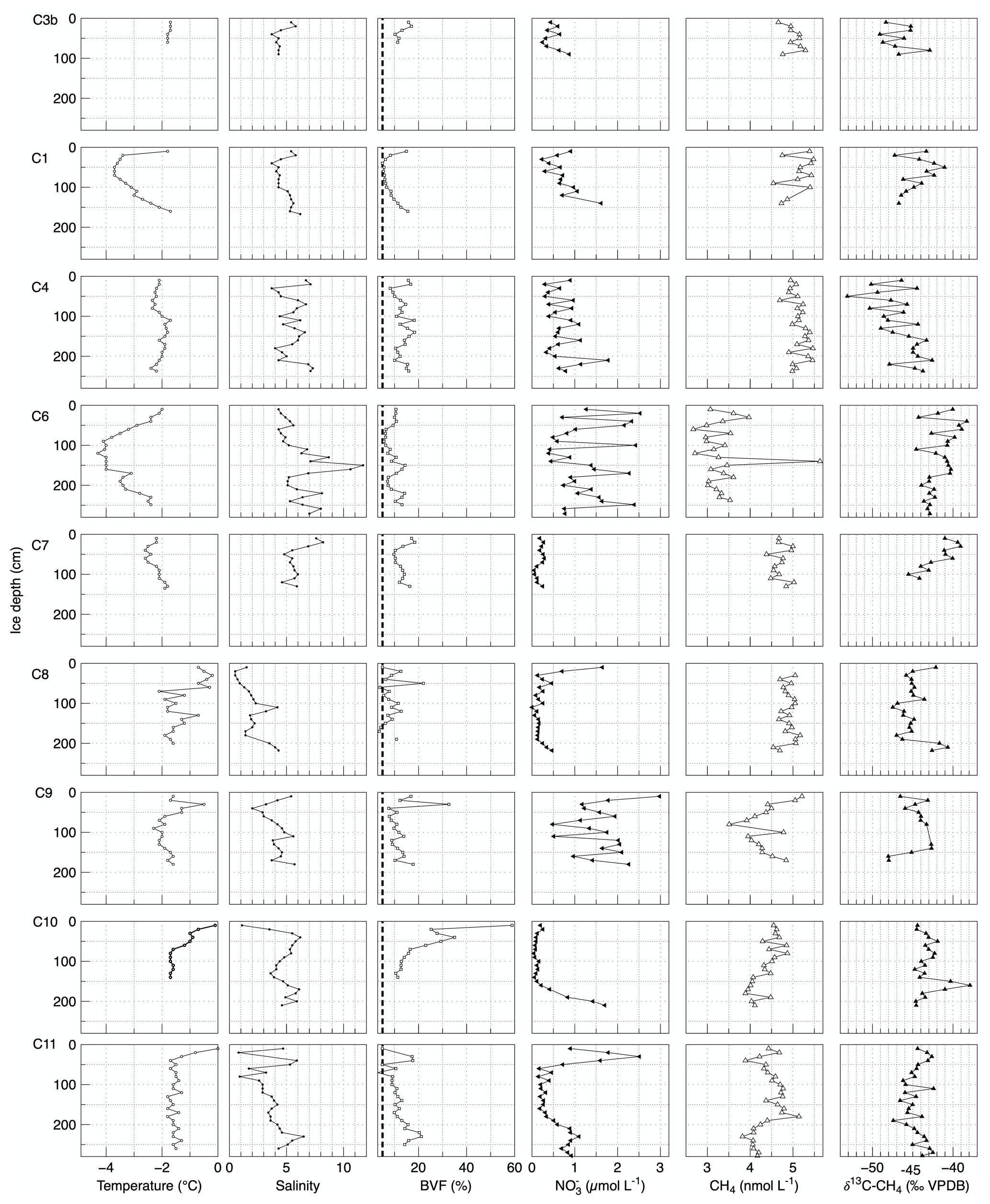
Figure 2Temperature, salinity, brine volume fraction (BVF), nitrate (NO), methane concentration (CH4), and the stable carbon isotopic signature of methane (δ13C-CH4) from sea ice cores taken across the ice floe. Dashed black line in BVF indicates when values are <5 %, corresponding to impermeable sea ice (Golden et al., 1998).
3.1.1 First year ice
Station C3b was characterized by thin FYI and used as “standard ice conditions” to compare with thicker ridged/rafted ice. In situ sea ice temperatures were almost homogenous towards the ice bottom (<100 cm) and varied only between −1.8 and −1.7 ∘C (Fig. 2). Salinity ranged from 3.7 to 5.8 with the highest values at 20 cm and homogenous from 40 cm down to the ice bottom. The BVF varied between 10 % and 15 %, with the upper part of the core (0–40 cm) being more permeable than the lower part, reflecting the surface melt onset. Nitrate concentration ranged between 0.24 and 0.87 µmol L−1, and it increased at the bottom of the ice. Methane concentration ranged from 4.7 to 5.5 nmol L−1 with the highest values in the middle of the core. The δ13C-CH4 values varied from −49.09 ‰ VPDB to −42.89 ‰ VPDB with no clear pattern.
3.1.2 Ridged/rafted ice with impermeable and permeable ice layers
Stations C1, C8, and C11 were characterized by impermeable ice layers in the middle of the core and permeable ice layers both at the top and bottom of the ice. In situ sea ice temperatures ranged from −3.7 to −0.2 ∘C. In general, the lowest values were found in the middle of the core (Fig. 2). Salinity varied from 0.5 to 6.2, showing an increase with ice depth. The BVF ranged from 3 % and 22 %, showing a general increase with ice depth and reflecting the onset of basal melt. Nitrate concentration ranged from 0.02 to 2.51 µmol L−1, and it increased at the bottom of the ice. Methane concentration ranged between 3.8 and 5.5 nmol L−1. In C1, the highest methane concentration coincided with low BVF. In C11, a pronounced decrease at the bottom of the ice coincident with an increasing nitrate concentration was detected, while in C8 a homogenously distribution within the ice was observed. The δ13C-CH4 values ranged from −47.48 ‰ VPDB to −41.05 ‰ VPDB. In impermeable ice layers of C1, we detected δ13C-CH4 values more enriched in 13C compared to the impermeable ice layers in C8 and C11. In permeable ice layers of both C8 and C11 we detected δ13C-CH4 values more enriched in 13C compared to permeable ice layers in C1.
Table 1Characteristics of the ice stations showing the information about the stations name, date of sampling during the ice drift in 2017, the ice thickness, snow thickness, and the stable carbon isotopic signature of methane (δ13C-CH4) values in brine sampled following the “sackhole” method (e.g., Gleitz et al., 1995). Brine samples were taken at stations C8, C10, C11 (one sample per station), and C9 (three samples).

3.1.3 Ridged/rafted ice with a water pocket
At station C6 we found an ice core that contained a “water pocket”, i.e., mixture of ice and water (slush), upon core extraction from 90–160 cm. In situ sea ice temperatures varied from −4.3 to −2 ∘C with the lowest values in the middle 90–160 cm of the ice core (Fig. 2). Salinity highly varied between 4.3 and 11.7, showing a general increase from top to bottom with the highest values from 100 to 170 cm. Over the cold middle layer, salinity was high with a pronounced peak of 11.7 at 150 cm. The BVF varied between 5.6 % and 15 %, with the highest permeability in the middle (90–160 cm, within the water pocket). Nitrate concentration ranged between 0.39 and 2.5 µmol L−1 and exhibited highly variable values towards the ice bottom. The methane concentrations were mostly homogeneous (approximately 2.7 nmol L−1) except for a spike of 5.6 nmol L−1 at 140 cm within the water pocket. The δ13C-CH4 values ranged from −44.57 ‰ VPDB to −38.29 ‰ VPDB. In the impermeable layers, we detected δ13C-CH4 values more enriched in 13C compared to the impermeable ice layers in C1, C8, and C11.
3.1.4 Ridged/rafted ice with fully permeable ice layers
Stations C4, C7, C9, and C10 were characterized by permeable ice layers throughout the ice cores. In situ sea ice temperatures varied from −2.6 to −0.1 ∘C (Fig. 2). Salinity values varied from 1.1 to 8.2 with no clear pattern found between the ice cores. The BVF varied between 7.5 % and 59 %, i.e., fully permeable. Nitrate concentration ranged between 0.04 and 2.98 µmol L−1 with a heterogenous vertical distribution except for C10 where an increase at the bottom of the ice was detected. Methane concentration ranged from 3.5 to 5.3 nmol L−1 with a homogenous distribution throughout the ice in C4 and C7. A decrease at the bottom of the ice coincident with an increasing nitrate concentration was observed in C10. By contrast, in C9 we observed high values at the top and at the bottom of the ice and a decrease in concentration in the middle of the core. The δ13C-CH4 values fluctuated highly from −53.12 ‰ VPDB to −37.89 ‰ VPDB. Overall, δ13C-CH4 values more enriched in 13C coincided with lower methane concentration.
3.2 Hydrographic characteristics of the seawater
During the ice drift, the bulk of waters in the upper 100 m was characterized as Polar Surface Water (PSW; σ0<27.70 and θ<0 ∘C; see, e.g., Rudels et al., 2000). The temperature (CT) was generally close to the freezing temperature and varied between −1.82 and −1.65 ∘C (average −1.79 ∘C) down to 60 m depth. Below 60 m, the temperatures increased steadily, ranging between −1.34 and −0.13 ∘C (average −0.75 ∘C) at 90–100 m depth (Figs. 3a and 4b). The absolute salinity (SA) varied from 33.82 to 34.39 g kg−1 (average 34.31 g kg−1) in the upper 60 m and between 34.45 and 34.63 g kg−1 (average 34.53 g kg−1) at 90–100 m depth. The freshest salinities where observed at stations 24-1 to 27-6 (sampled 7–10 June) in connection with slightly increased temperatures in the upper 40 m. The upper 60 m of the water column were relatively weakly stratified yet exhibited alternating patches of stable stratification as shown by the Brunt–Väisälä (buoyancy) frequency (Gill, 1982) in Fig. 4c. The observed conditions were in line with earlier reported values from this area and season (Meyer et al., 2017; Rudels et al., 2000).
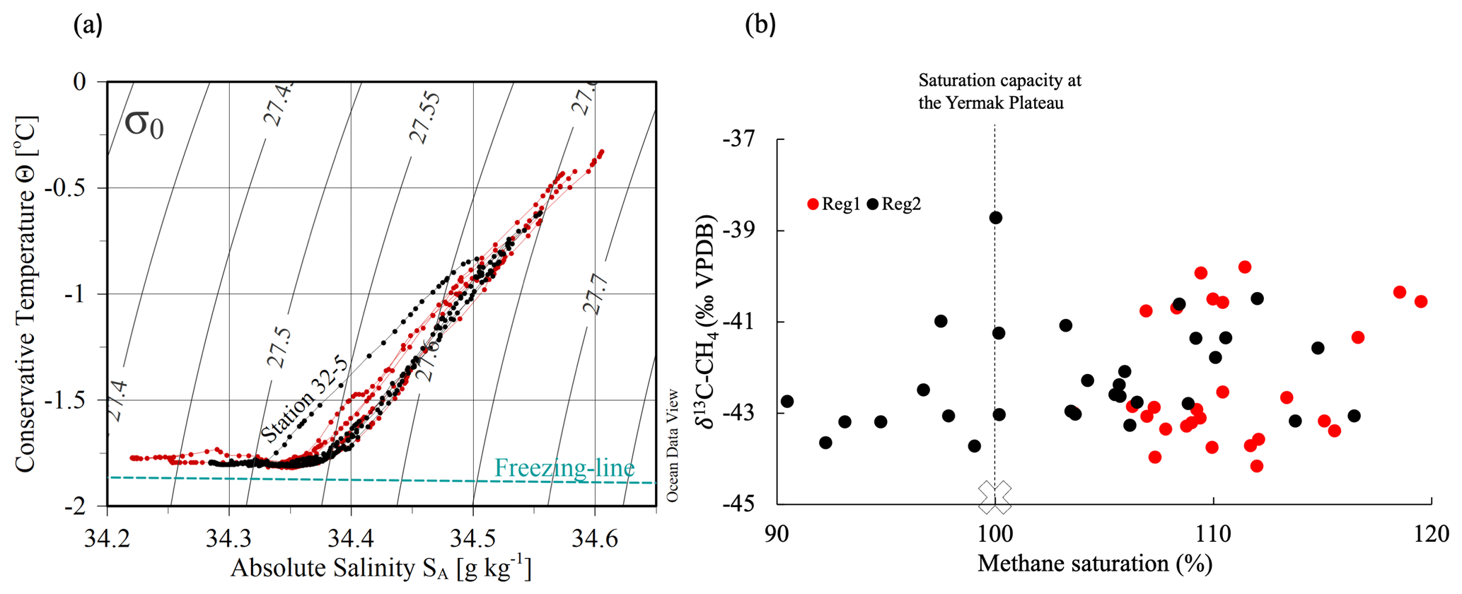
Figure 3(a) Temperature-salinity (TS) diagram for the upper 100 m at the methane sampling stations during the ice drift. In red are the stations located over the Yermak Plateau (Region 1), and in black are those over the Yermak Plateau eastern flanks (Region 2). The dashed line indicates the salinity dependence of the freezing temperature. (b) Methane saturation vs. the δ13C signature of methane in seawater. Red and black colors indicate the regions and the dashed line the saturation capacity (100 %) at the Yermak Plateau (see Sect. 4.2). The atmospheric background signature of methane of −45 ‰ VPDB is marked with a cross.
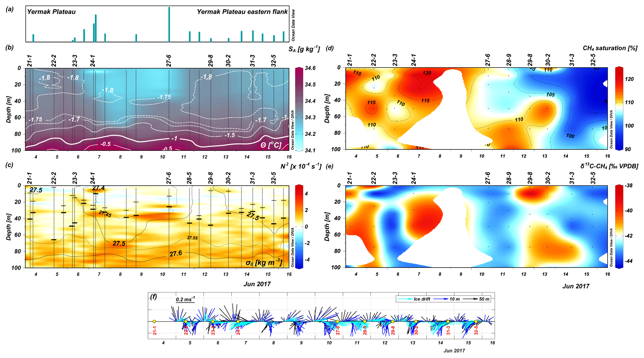
Figure 4Seawater properties in the upper 100 m along the drift track. The labels on top of panel (b)–(e) denote the CTD stations where methane was sampled in the seawater. Additional CTD casts were used in (a)–(c) as indicated by vertical black lines but otherwise not further presented in this study. (a) Degree of ice melt estimated from the TS profiles (Sect. 3.2). Due to the early melt season, the length scale of the bars was omitted to emphasize the use of this measure only as a qualitative guidance. (b) Absolute salinity (g kg−1) overlaid with isothermals of conservative temperature (∘C). (c) Brunt–Väisälä Frequency (10−4 s−1) overlaid with isopycnals of potential density anomaly (kg m−3, 0 dbar ref. pressure). Positive N2 values indicate stable stratification. Horizontal black bars show the mixed layer depths estimated for two different density thresholds (upper bar: 0.003 kg m−3; lower bar: 0.01 kg m−3; see Sect. 3.2). (d) The temporal development of methane saturation (color bar) overlaid with contours of saturation levels and (e) of the δ13C signature of methane (‰ VPDB). (f) Hourly vectors of the horizontal speed and direction of the ice floe and the underlying waters at 10 and 50 m depth, respectively (water velocities unavailable before 5 June). The vector magnitudes follow the length scale in the upper left corner, and north is upward. Yellow dots indicate the methane sampling stations.
To help us characterize the stations which, in general, showed only the first signs of seasonal melt (and a few still with winter conditions prevailing), the mixed layer depth (MLD) was calculated for two density thresholds (Meyer et al., 2017); the depth where the density difference was 0.003 kg m−3 relative to the density at 3 m depth was used to indicate the in-season MLD formed by the first melting, and a difference of 0.01 kg m−3 relative to 20 m depth was used for the depth of the past winter convection (see Fig. 4c). The melt-affected MLD (Δρ=0.003 kg m−3) was 19 m on average over the entire drift, while the deeper MLD (Δρ=0.01 kg m−3) averaged to 37 m. However, the variation between stations was rather large (SD ∼ 11 m) for both these estimates. Among the stations sampled for methane, the “winter-layer” was the deepest at station 22-2 (66 m) and the shallowest at station 27-6 (26 m).
The salinity and temperature characteristics were used in the winter to summer transition formula of Peralta-Ferriz and Woodgate (2015; their Eq. 2) to estimate the ice thickness required to transform a winter mixed layer into a thinner fresher summer mixed layer (Fig. 4c). This calculation naturally makes better sense by the end of the melting season but was used here as a quick means to compare the ice-melt status at our stations, as found by our observed seawater properties, and the values of sea ice density (= 920 kg m−3) and sea ice salinity (∼ 6) given in Peralta-Ferriz and Woodgate (2015). The largest amount of melting was indicated at stations 27-6 and 24-1, coincident with the freshest salinities and the largest differences between observed temperatures and the freezing point (Fig. 4b).
3.3 Methane concentration, saturation, and the δ13C-CH4 in the seawater
In the seawater, the methane concentrations varied from 3.3 to 4.8 nmol L−1 corresponding to saturations between 90 % and 120 % relative to the atmospheric background. In general, the highest methane concentration was observed during the first part of the drift over the Yermak Plateau (YP). During the latter part of the drift over deeper waters along the slope, methane concentration decreased. The δ13C-CH4 values in the seawater ranged between −44.17 ‰ VPDB and −38.73 ‰ VPDB. A heterogeneous distribution was observed with no clear pattern. Nevertheless, values more enriched in 13C coincided with higher methane saturation (Fig. 3b).
Our study traces the methane pathways within drifting sea ice and between the sea ice and the underlying seawater just at the start of the melt season. The measurement campaign took place over a seemingly small geographic area of the Yermak Plateau, but, judging by the variation in methane saturation levels in seawater, it comprised two distinct “regions” (Figs. 1b and 3b). Our drift started in the northeastern, relatively shallow parts (depth 800–1000 m; denoted Region 1) of the Yermak Plateau. Windy days on 9–11 June brought us into deeper waters over the eastern flanks of the plateau. During the last days from 11–15 June (with mainly northeasterly winds), we drifted southwestward along the slope (depth 1300–1500 m; denoted Region 2) until it was time to abandon the floe and return to harbor.
Our ice floe consisted of both thin FYI and ridged/rafted ice of various thicknesses and internal structure, and this heterogeneity among our ice cores was reflected by differences in the melting process. In this context, FYI was permeable throughout the entire ice column, while deeper segments of complex structures like ridged or rafted ice were still impermeable. We used ice permeability as the indicator of the stage of melt to follow the methane pathways as ice permeability determines the capacity for methane storage in sea ice. Hence, impermeable layers may be characterized by relict winter conditions, while permeable layers show signs of the ongoing melt, i.e., the current late spring conditions.
Below, we first discuss potential initial (source) methane signals still preserved within impermeable layers in the sea ice. Also, we follow the pathways of methane when melt starts, focusing on the exchanges between the ice and the seawater underneath the floe. Secondly, we discuss methane saturation deviations in the upper 100 m of the water column along our drift path.
4.1 Fate of methane transported by different sea ice types
When the BVF drops below 5 %, sea ice becomes impermeable (Golden et al., 1998), leading to restricted gas exchange (Loose et al., 2017; Rutgers van der Loeff et al., 2014). Building off this principle, we searched for impermeable layers as relicts of winter conditions to highlight the fate of methane enclosed within drifting ice. We detected winter (i.e., pre-melt) conditions in two different types of “sandwich structures”: (i) an impermeable layer in the middle of the ice separated by permeable layers on the top and bottom of the ice and (ii) a permeable layer (water pocket) enclosed by impermeable layers on the top and bottom of the ice (Fig. 5).
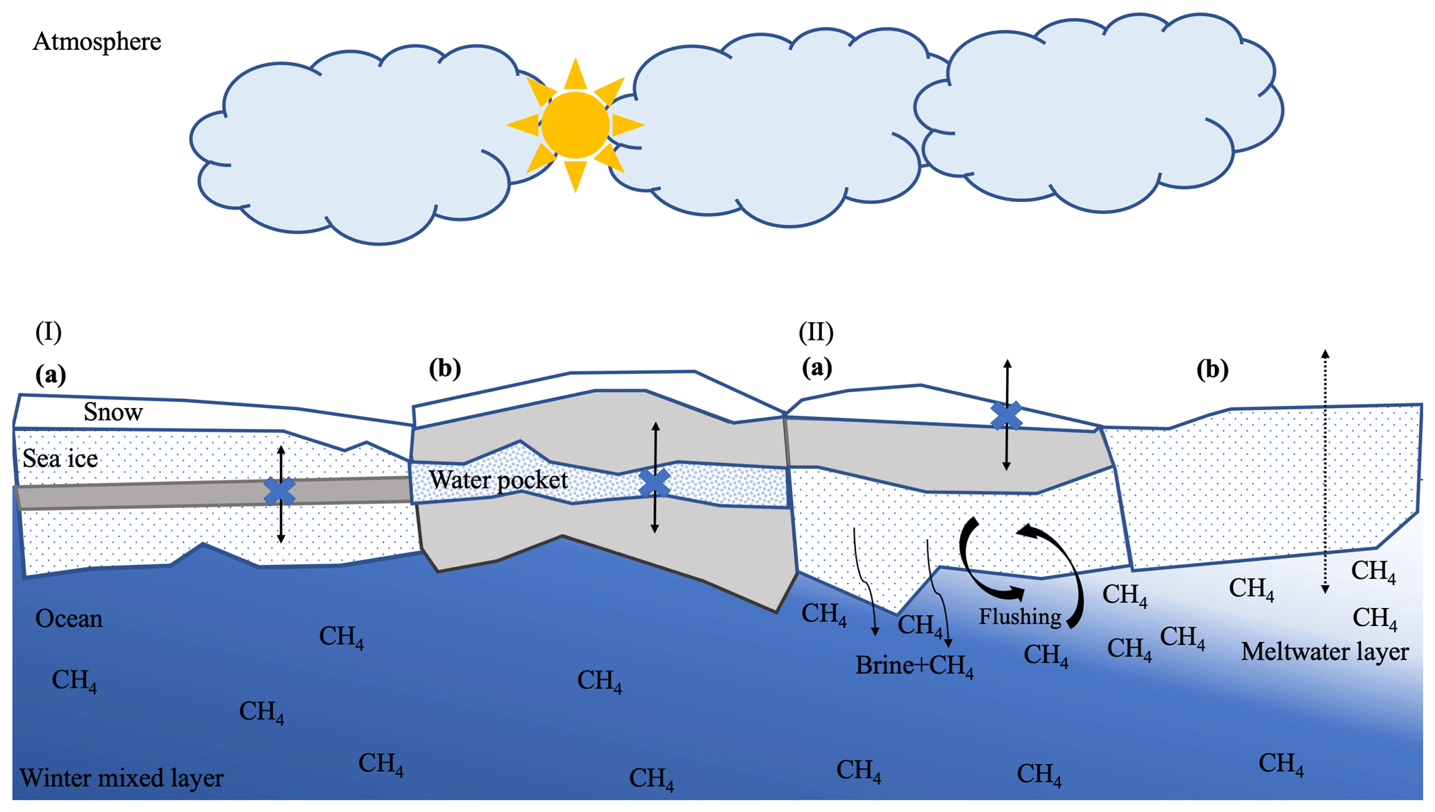
Figure 5Potential pathways of methane in sea ice with varying impermeable (indicated in grey) and permeable sections (in white with blue dots), i.e., winter (I) and spring (II) conditions. I (a) Relicts of the initial methane signal (source) entrapped in impermeable ice layers. Impermeable intermediate sea ice layers act as a barrier for the upward/downward transport of methane (black arrow overlaid by a blue cross). (b) Residual methane signal after methane oxidation occurred in permeable sea ice layers (“water pocket”), enclosed by impermeable ice layers (see Fig. 6). II (a) When basal melt starts, but the top layer still is impermeable and with snow cover (white layer on top of the ice), downward brine transport initiates release of dissolved methane. Flushing events trigger methane released into the ocean (see Sect. 4.1.3). (b) Unrestricted migration of methane in permeable sea ice layers (dotted black arrow). Ongoing sea ice melt, when freshwater from melted sea ice is released into the water underneath, resulting in a meltwater layer where methane remains sustained during late spring. Methane (CH4) annotation indicates concentration. Color gradient in the ocean reflects the increasing stratification during the seasonal evolution of the upper part of the winter mixed layer (in blue) into a fresh meltwater layer (in white).
4.1.1 Methane source signals in relicts of impermeable sea ice
In isolated impermeable layers, the methane concentration was higher relative to the atmospheric background concentration. In addition, the stable carbon isotopic signature deviated from the atmospheric background value (see C1 and C11 in Figs. 2 and 6). As both results corroborate restricted gas exchange during the ice drift, we suggest that methane preserved in these impermeable layers was trapped during ice formation. Methane uptake in sea ice occurs by freeze-up events of supersaturated seawater (Crabeck et al., 2014; Damm et al., 2018). Thus, the initial methane inventory trapped in impermeable layers may have its source far from the present location of the ice floe. Large fractions of sea ice that reach the Fram Strait originate from the Laptev Sea (Krumpen et al., 2016, 2019, 2020), while the Siberian shelf waters are known to be supersaturated with methane (Thornton et al., 2016). The methane concentration in waters covered by sea ice in the Laptev Sea shelf area can be up to 3 orders of magnitude higher than atmospheric background concentrations (Sapart et al., 2017). The origin of the excess methane is microbial, being produced in sediments and partially oxidized before reaching the seawater (Sapart et al., 2017). We attribute the offset in stable isotope ratios in our sea ice compared to the seawater above the sediment from Sapart et al. (2017) to either fractionation that occurred during freeze-up or microbial methane consumption that took place in the seawater before uptake into sea ice. To address these hypotheses, future studies should directly compare both sea ice and water, particularly during ice formation.
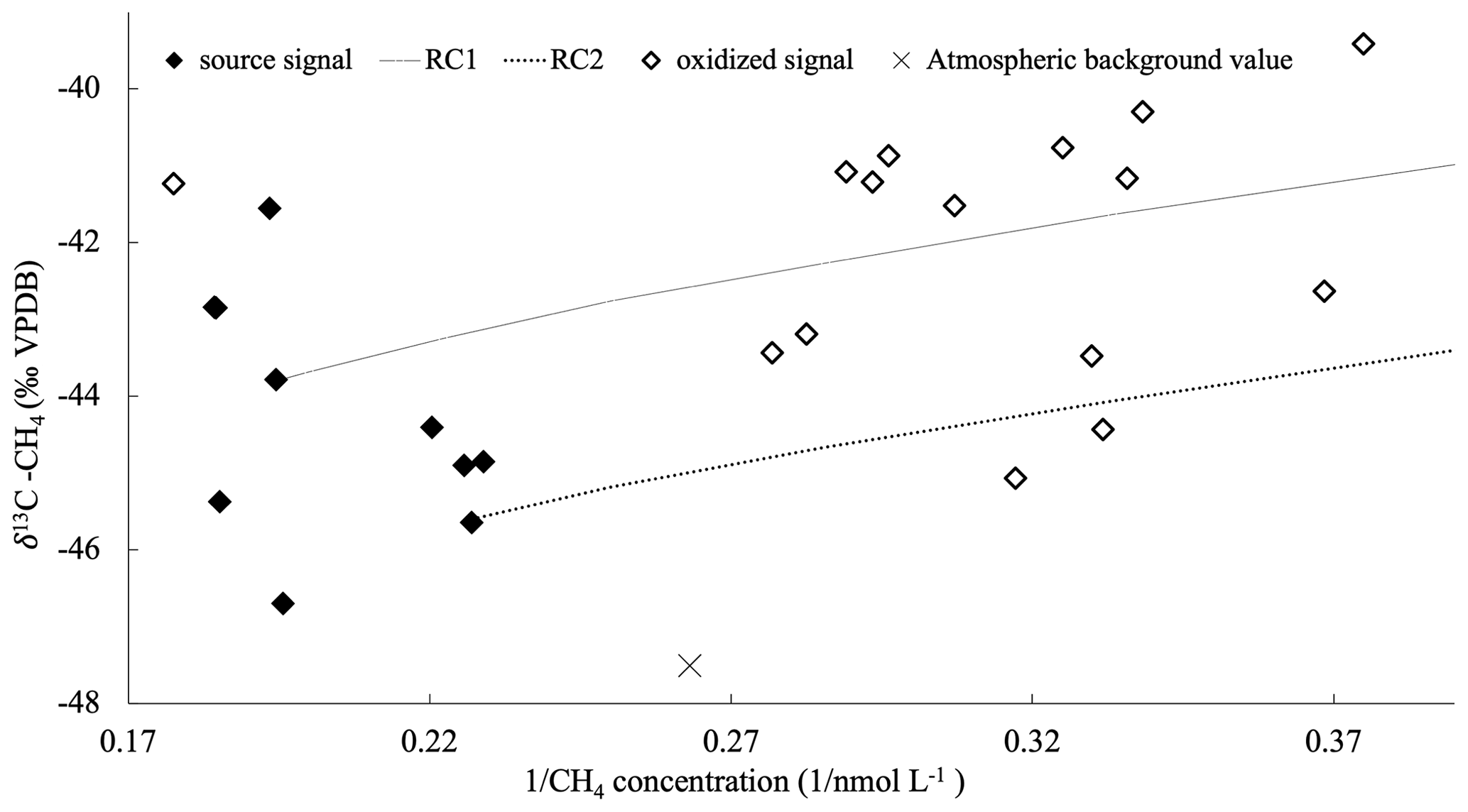
Figure 6The reciprocal of methane concentration vs. the δ13C-CH4 in sea ice. Methane enclosed in impermeable layers (black diamonds) deviates from the atmospheric background value (cross) and reflects the initial methane (source) signal being unchanged and stored in impermeable sea ice during the drift. The source signal also represents the starting point for the calculation of potential methane consumption. The residual methane (open diamonds), i.e., a pool with less methane concentration but more enriched in 13C, is formed by methane consumption in a permeable layer enclosed by impermeable ice layers in ridged/rafted ice. Two Rayleigh curves (RC1: dashed line; RC2: dotted line) have been calculated with two different initial isotopic signatures (−44 ‰ VPDB and −46 ‰ VPDB), respectively; α is 1.004 (see Sect. 4.1.1 and 4.1.2).
4.1.2 Methane oxidation in permeable sea ice protected by impermeable layers
We observed an enclosed permeable layer surrounded by impermeable sea ice in a complex ridged/rafted ice structure (C6 in Fig. 2; Fig. 5). This type of ice structure is formed by flooding events from storm-induced floe breakup and ridge formation during subsequent floe consolidation (Provost et al., 2017). During such events, seawater becomes trapped in ridged/rafted ice structures creating more saline conditions within certain layers therein. Subsequently, the enhanced salinity sustains permeable layers that are protected by impermeable sea ice enveloping them. Within the enclosed permeable ice layers, we detected methane enriched in 13C compared to the source methane trapped in impermeable sea ice. As the methane concentration correspondingly dropped down, we conclude that methane consumption occurred in this protected and permeable saline environment (Fig. 6). During microbial methane consumption, isotopic fractionation occurs as methane 12C is preferentially consumed compared to 13C, which, in turn, induces a 13C enriched residual methane pool when consumption ceases (Coleman et al., 1981).
A potential isotopic fractionation during methane consumption is corroborated by a Rayleigh curve calculated as follows:
where α is the isotopic fractionation factor, f is the fraction of the residual methane remaining in the enveloped permeable layer, and the initial isotopic composition (δ13C-CH4)0 corresponds to the isotopic composition of methane detected in impermeable layers (source signal). Using a Rayleigh fractionation model, we assume that the methane reservoir has no further sinks or inputs and no mixing occurs (Mook, 1994). In summary, pockets of permeable ice enclosed by impermeable ice can act as a favorable microbial environment for methane consumption. As a potential response to the expected future thinning of the sea ice, an increased number of permeable pockets formed during ice ridging may lead to favored methane oxidation therein. Under these circumstances, we suggest that the methane pathways can be modified; i.e., sea ice may be considered as a sink for methane.
4.1.3 Fate of methane trapped in sea ice when ice develops permeable layers
The vertical distribution of impermeable and permeable layers during ongoing ice melt is associated with different methane pathways (Zhou et al., 2014). As the melting front advances vertically trough the ice, the brine networks within the sea ice expand, transporting the methane dissolved in the brine downwards. When snow cover diminishes and the sea ice surface is permeable, sea-ice-to-air emissions are most likely enhanced, and methane initially entrapped in the sea ice can be released to the atmosphere. Accordingly, both the sea ice permeability and the snow thickness on top of the ice are particularly important as they determine the methane flux variations across the sea-ice–air interface (He et al., 2013). However, at the time of our sampling, we detected impermeable layers on top of the ice covered by a thick layer of snow (e.g., Table 1; Fig. 2, C11). We therefore assume that the sea-ice–air flux was inhibited at this stage of the melt.
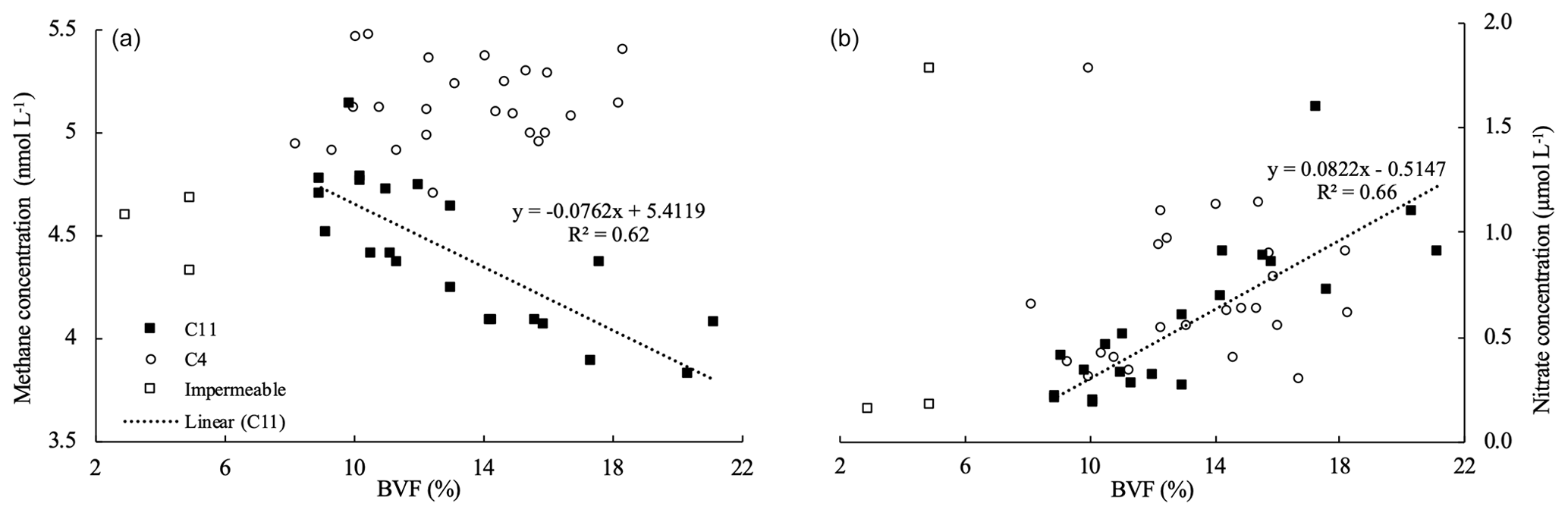
Figure 7(a) Methane and (b) nitrate concentration vs. brine volume fraction (BVF) at C11 and C4, respectively. In C11, methane is inversely correlated (R2=0.62), while nitrate is correlated (R2=0.66) with increasing BVF. This trend shows that methane is released from ice, while nitrate is taken up. In station C4, correlation is missing when sea ice is fully permeable. C4 shows a homogenously distribution of methane, as well as nitrate, and a higher concentration than in C11 caused by the flushing of seawater charged with methane and nitrate into the sea ice. The three outlier points (impermeable ice layers) have been removed for the correlations.
At the bottom of the sea ice, brine is released into the ocean when basal melt starts (Eicken, 2002), discharging the dissolved methane into the seawater (Damm et al., 2015). Hence, increased ice permeability at the ice bottom triggers methane release. This circumstance eventually causes low methane concentrations at the bottom of the ice, a scenario evident at C11 (Fig. 2). Additionally, it coincides with an increase in nitrate at the ice bottom. The correlation of these variables in C11 corroborates methane release (Fig. 7). Remarkably, the nitrate concentration was 5 times higher in the permeable layers at the bottom of the ice core compared to the impermeable layers on top of the ice, which suggests a source associated with the flushing of seawater into the sea ice. Flushing here refers to the “washing out” of salty brine by relatively fresh surface meltwater that percolates into the pore space (Untersteiner, 1968; Vancoppenolle et al., 2013). In addition, flushing may be induced by the mechanical entrainment of the water underneath the ice due to the rough ice bottom being “dragged” at varying speeds and in various manners. Nitrate availability in seawater directly underneath the ice during the time of the drift (5 µ mol L−1 at 2 and 3 m depth) further supports flushing events being the reason for the enhanced concentrations at the ice bottom. In this context, we conclude that methane discharge into the ocean is likely to be the preferential pathway at this time of the year (Fig. 5).
Furthermore, it is necessary to refer to the methane pathways in the opposite scenario, i.e., when permeable conditions develop throughout the entire ice column and snow on top is nearly all melted. In this context, we detected ice cores with methane and nitrate concentrations homogenously distributed within the ice (e.g., C4 in Fig. 7). This circumstance is also triggered by flushing events, but unlike C11, supersaturated seawater is flushed into permeable ice, and consequently, the concentrations of both methane and nitrate are enhanced therein. The non-existent correlation between methane and nitrate corroborates that supersaturated seawater is flushed into permeable ice (Fig. 7). However, under the “extreme” scenario of highly permeable ice, i.e., latest stage of melt, and no snow coverage on top of the ice, the sea-ice-to-air emissions would need to be considered.
4.2 Dissolved methane in polar surface water (PSW)
Methane dissolved in the upper 100 m of the water column was not in equilibrium with the atmospheric background values. Indeed, methane was found across the range from slightly under- to supersaturated relative to the saturation capacity of seawater at the Yermak Plateau (YP, 100 %; Fig. 3b), calculated with in situ ∘C and SP=34.19, which corresponds to a saturation concentration of 4.0 nmol L−1. The atmospheric background signature of methane of −45 ‰ VPDB corresponds to the atmospheric δ13C-CH4 value (−47 ‰ VPDB; Quay et al., 1991) corrected by the kinetic isotopic fractionation effect (Happell et al., 1995). In addition, methane was enriched in 13C compared to the atmospheric background signature (Fig. 3b). The deviation in the δ13C-CH4 values from this background value reflects the influence of methane released from sea ice.
The surface waters in this region are expected to be undersaturated due to increased solubility capacity inferred by cooling and freshening of their source waters (Damm et al., 2018). Conspicuously, we observed mainly supersaturation in seawater. The estimated enhancement of the solubility capacity of about 10 % is in line with the long-term cooling and freshening effect on the Atlantic Water forming the PSW (Rudels et al., 2000). All CTD profiles during the drift showed that the upper 100 m were consistently characterized as PSW, but it is unclear if these formed remotely in the Eurasian Basin and returned with the TPD towards the Fram Strait (Damm et al., 2018; Rudels, 2012) or if they formed more locally over the Yermak Plateau or in the adjacent Sofia Deep. Nevertheless, the final effect of cooling Atlantic Water with original characteristics from the major inflow region (θ>3 ∘C, SP>35; Orvik and Niiler, 2002) to the T/S observed at the drift site would be the same, with a major part of the solubility enhancement being due to the cooling (9 %) while the rest is due to freshening.
In general, methane excess in seawater could also originate from sediments. In our case, a potential source could have been the area west of Svalbard (Sahling et al., 2014; Smith et al., 2014; Westbrook et al., 2009). However, methane released from sediments are laterally transported in the deep ocean and do not reach the surface waters (Damm et al., 2005; Graves et al., 2015; Silyakova et al., 2020). Hence, the surface waters remain unaffected by methane released from sediment sources further south. Based on our data and the regional oceanographic conditions, we suggest that methane released from sea ice is a source of the observed excess in the PSW.
In the following sections, we discuss these findings and the relationship of the methane saturation levels to the characteristics of the underlying waters with a focus on the interaction with the sea ice.
4.2.1 Methane supersaturation in PSW by release from sea ice
Even though the area of our drift was relatively small (see Fig. 1b), there were pronounced differences in methane supersaturation levels in the seawater samples (Fig. 4d). When ice starts to melt, brine is released into the ocean (Eicken, 2002), as well as the methane dissolved in the brine (Damm et al., 2015). The CTD profiles at most of the methane sampling stations indicate the typical-for-spring onset of heating from above and an associated freshening due to initial melting (Fig. 4b). Even if it is not certain that all the warming and freshening may be attributed to our own floe, it has drifted over patches of water with the potential to trigger basal melt. In our ice core brine samples we found a δ13C signature of methane enriched in 13C (Table 1). Enrichment in 13C, compared to the background value, was also observed in the seawater samples (Fig. 3b), and we therefore conclude that brine release had occurred. For example, at station 24-1, a warmer and fresher (ΔT∼0.03 ∘C, ΔS∼0.01 g kg−1) layer down to about 40 m contained a high methane supersaturation level, reflecting both sea ice melt and sea ice methane release (Fig. 4a to d).
An early melt stage (initiated basal melt) would be indicated by a low degree of dilution of the released methane since only small amounts of meltwater are available at first. This is observed in the methane supersaturation (up to 20 %) relative to the saturation capacity at the YP. Additionally, the varied δ13C-CH4 values detected in seawater corroborate sea ice methane release (Fig. 3b).
Hence, the methane supersaturation levels in PSW, at this time of the year, are likely to be sea-ice-sourced, and the ongoing ice melt process influences this excess.
4.2.2 Variability in methane saturation levels in PSW by oceanographic processes
During our drift, the stations were affected by varying degrees of ice melt, i.e., a varying degree of warming and freshening, with implications on the stratification and the potential to preserve the released methane (Fig. 4a to e). Methane released from sea ice into a shallow mixed layer would be mixed and diluted to a certain degree but, nevertheless, would be relatively well preserved within the layer, like the supersaturation observations at stations 29-8 and 30-2 (at 2 m). This assumption is corroborated by values more enriched in 13C associated with methane concentration “hot-spots” underneath the ice (Fig. 4d and e). Methane released into a deep mixed layer would have the potential to spread to a greater depth, as detected at station 22-2 where the deepest calculated “winter mixed layer” was detected (Fig. 4c to e).
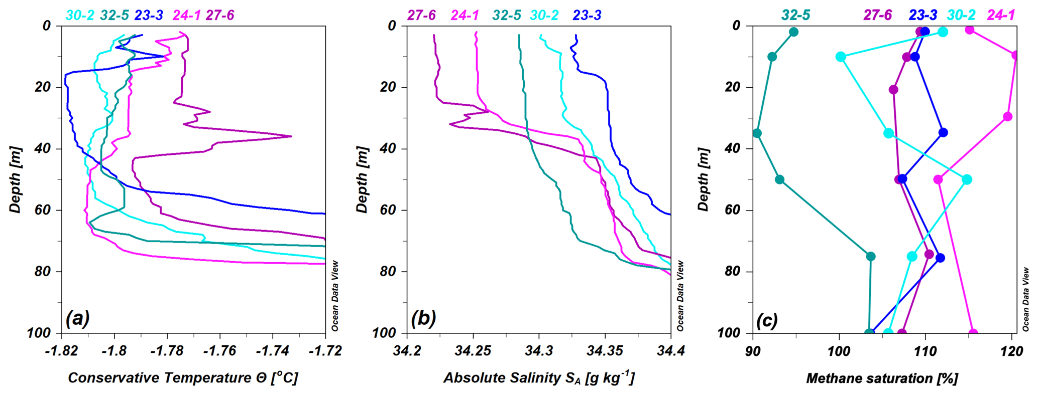
Figure 8Profiles of (a) conservative temperature (∘C), (b) absolute salinity (g kg−1), and (c) methane saturation (%) for some of the sites with warmer and fresher waters in the topmost layers, indicating the onset of the seasonal ice melt to various degrees. The stations are indicated by the labels on top of each panel.
At the stations with large melt, the methane excess seemed to be preserved in the meltwater layer with the help of the increased stratification underneath: down to about 40 m depth at station 24-1 and down to 20 m depth at station 27-6 (Fig. 4a to d). However, the conditions at station 27-6 are more complex than at the “normal-looking” station 24-1, with a relatively warm and salty layer interleaving at 25–40 m depth reflected in a decreased methane saturation level at these depths (Fig. 8).
Furthermore, the spatial variation of supersaturation levels could also be due to differences in the advection speed and direction of the drifting floe relative to the traversed waters. When sea ice and water travel together (same speed and direction), the contact time between the floe and the water is prolonged, and we imagine a well-coupled system between sea ice and the underlying water. The advection of ice and water is summarized by the vectors in Fig. 4f, still with the prominent tidal signal contained. Both the average and maximum speeds of water were similar at the two depths (0.03 and 0.20 m s−1 at 10 m and 0.02 and 0.25 m s−1 at 50 m, respectively) and lower than for the ice floe (0.09 and 0.30 m s−1). Nevertheless, it is evident that the interplay between ice and water motion is very variable and due to both the atmospheric (winds) and oceanic forcing (currents).
During the first part of the drift (over shallower grounds) the “back-and-forth” rotational nature of the ice and water movements seems to have contributed to the methane supersaturation being sustained in the water along the drift. In contrast, during the latter part of the drift there was a more advective and unidirectional nature to the flow along the sloping topography of the YP's southeastern flank (stations 29-8 to 32-5; Fig. 4f). Ice and water were seemingly traveling in the same direction at comparable speeds, and we therefore expected a similar pattern for these stations. However, lower methane saturation levels were observed, e.g., at stations 31-3 and 32-5, and perhaps the unidirectional state was variable enough to prevent us from fully catching the methane signal from melting ice. Between 40 and 75 m at stations 29-8 and 30-2, more methane was observed in slightly colder and saltier water (Fig. 4b and d). In summary, the fate of the sea-ice-sourced methane in the surface waters depends both on how stratification acts to retain this excess in the surface layer and on the spatial and temporal coherence of the coupled sea-ice–ocean system during the drift.
The type and structure of Arctic sea ice affect the capacity for methane storage (Fig. 9). Our study provides evidence that ridged/rafted sea ice structures create environments where methane oxidation occurs during the Transpolar Drift, eventually acting as a sink for methane. On one hand, a faster sea ice drift (Spreen et al., 2011) resulting from a thinning ice cover may reduce the time for methane to be oxidized within the ice, leading to changes in the methane pathways. Further research should consider rate measurements of methane oxidation mainly in ridged/rafted ice structures to determine the long-term impact of this process. On the other hand, with an accelerated sea ice transport, methane taken up in sea ice will be transported to remote areas and released in surface waters of regions not yet affected by methane excess. We suggest that future studies should be focused on sea ice formation on different arctic shelves to validate the importance of methane uptake during ice formation.
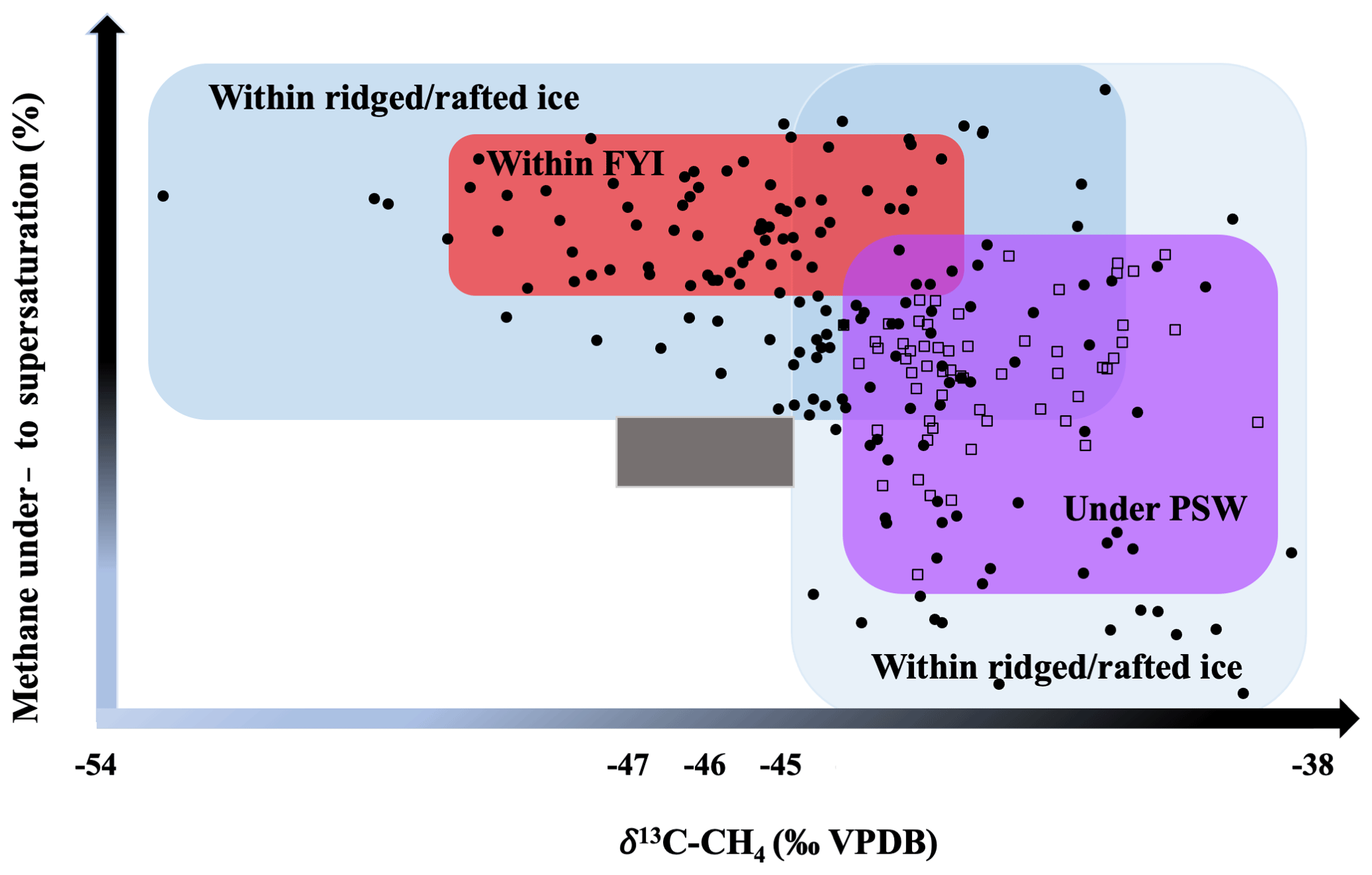
Figure 9Variability in the methane inventories within different ice types on our ice floe and PSW underneath. The grey rectangle shows the atmospheric background signature.
For the season of late spring we propose methane release from sea ice into the meltwater layer as the predominant pathway. At this time, basal melt is occurring, and the top of sea ice loaded with methane is still impermeable. Tracing the overall transfer of methane from sea ice into the ocean is important for understanding and quantifying the dynamic contribution of sea ice for the methane source–sink balance. It is not yet clear which process contributes the largest amount of methane release from sea ice: the brine release during freeze-up in winter or during melting in spring. Both processes need to be considered, and the amount of methane must be quantified. Extended analyses and robust numerical modeling of these processes within the entire sea-ice–ocean (and atmosphere) system are needed to improve our ability to predict the consequences of the methane source–sink balance modifications in the Arctic Ocean.
Our study suggests that the excess of methane in PSW during late spring is sea-ice-sourced. The degree of ice melt regulates this excess through the amount of meltwater added to the surface layer by (a) ruling dilution throughout the melting period and (b) affecting the stratification and the potential for the sea-ice-released methane to be retained in the meltwater layer. The meltwater layer also inhibits the sea-to-air flux from deeper levels and increasingly so during its seasonal development (i.e., freshening and warming) when it deepens through various mixing processes. Further studies should estimate the amount of methane released into the atmosphere by the sea-ice-to-air flux compared to the amount released by brine rejection into the marine environment.
The relative velocities of the ice and water, the influence of stratification on methane signal retention in the surface waters, and the impact of mechanical mixing from, for example, winds and tides are important factors for the evolution of sea-ice-induced methane excess in seawater underneath the ice. Dedicated studies for these processes are needed to better understand their relative importance for this context.
Finally, as long-term consequences, we consider the effects of an increased ocean heat content leading to enhanced ice melt and, hence, more freshwater discharged into the surface layer. Within the surface layer itself, a larger amount of freshwater would lead to an increased dilution effect on the methane content. The sink capacity of the surface waters for sea-ice-released methane may be increased either by dilution or by mechanical mixing processes. A fresher (and perhaps thicker) surface layer “cap” than today could further inhibit the exchange of methane between the subsurface ocean layers and the atmosphere through stronger stratification/isolation relative to ice below water. Thus, any methane excess in the waters below this “cap” would be disconnected from the atmosphere and be subject to further mixing with surrounding waters. Especially vulnerable for such changes are the areas beyond the current inflow area in the Eurasian basin, where the effect of the “Atlantification” is expected to be enhanced (Polyakov et al., 2017, 2020). Further work is required to investigate the spatial and temporal effects of the expected increase in ice-free waters in summer to methane pathways during the melt season.
The CTD data are available at https://doi.org/10.1594/PANGAEA.885442 (Nikolopoulos et al., 2018).
The biogeochemical data will be available on PANGAEA.
JV wrote the manuscript. JV and ED carried out the geochemical analyses and AN the oceanographic analysis. All authors contributed to the interpretation of the data and to the manuscript text and figures.
The authors declare that they have no conflict of interest.
We sincerely acknowledge the support of the captain and crew of RV Polarstern cruise ARK-XXXI/1.1 for their professional support at sea. We are thankful to one anonymous reviewer for constructive comments on the manuscript and to Michael Angelopoulos for improving comments on language. We also thank Ronny Engelmann for his support with the ice coring.
This research has been supported by the Alfred Wegener Institute Helmholtz Centre for Polar and Marine Research (grant no. AWI_PS106_00), National Agency for Research and Development (ANID)/Scholarship Program/Becas de Doctorado con acuerdo bilateral en el extranjero CONICYT-DAAD/2016-62150023, and the Deutscher Akademischer Austauschdienst (grant no. 91609942).The article processing charges for this open-access publication were covered by the Alfred Wegener Institute, Helmholtz Centre for Polar and Marine Research (AWI).
This paper was edited by Christian Haas and reviewed by one anonymous referee.
Coleman, D. D., Risatti, J. D., and Schoell, M.: Fractionation of carbon and hydrogen isotopes by methane-oxidising bacteria, Geochim. Cosmochim. Ac., 45, 1033–1037, 1981.
Cox, G. F. N. and Weeks, W. F.: CRREL Report 82-30, Equations for Determining the Gas and Brine Volumes in Sea Ice Samples, J. Glaciol., 29, 306–316, 1983.
Crabeck, O., Delille, B., Rysgaard, S., Thomas, D. N., Geilfus, N.-X., Else, B., and Tison, J.-L.: First “in situ” determination of gas transport coefficients (, DAr, and ) from bulk gas concentration measurements (O2, N2, Ar) in natural sea ice, J. Geophys. Res.-Oceans, 119, 6655–6668, https://doi.org/10.1002/2014JC009849, 2014.
Damm, E., Mackensen, A., Budéus, G., Faber, E., and Hanfland, C.: Pathways of methane in seawater: Plume spreading in an Arctic shelf environment (SW-Spitsbergen), Cont. Shelf Res., 25, 1453–1472, https://doi.org/10.1016/j.csr.2005.03.003, 2005.
Damm, E., Rudels, B., Schauer, U., Mau, S., and Dieckmann, G.: Methane excess in Arctic surface water-triggered by sea ice formation and melting, Sci. Rep., 5, 16179, https://doi.org/10.1038/srep16179, 2015.
Damm, E., Nomura, D., Martin, A., Dieckmann, G. S., and Meiners, K. M.: DMSP and DMS cycling within Antarctic sea ice during the winter-spring transition, Deep. Res. Pt. II, 131, 150–159, https://doi.org/10.1016/j.dsr2.2015.12.015, 2016.
Damm, E., Bauch, D., Krumpen, T., Rabe, B., Korhonen, M., Vinogradova, E., and Uhlig, C.: The Transpolar Drift conveys methane from the Siberian Shelf to the central Arctic Ocean, Sci. Rep., 8, 4515, https://doi.org/10.1038/s41598-018-22801-z, 2018.
Eicken, H.: Tracer studies of pathways and rates of meltwater transport through Arctic summer sea ice, J. Geophys. Res., 107, 8046, https://doi.org/10.1029/2000JC000583, 2002.
Fer, I., Müller, M., and Peterson, A. K.: Tidal forcing, energetics, and mixing near the Yermak Plateau, Ocean Sci., 11, 287–304, https://doi.org/10.5194/os-11-287-2015, 2015.
Gill, A. E.: Atmosphere-Ocean Dynamics, International Geophysics Series, vol. 30, Academic Press, USA, ISBN 0-12-283522-0, 666 pp., 1982.
Gleitz, M., v.d. Loeff, M. R., Thomas, D. N., Dieckmann, G. S., and Millero, F. J.: Comparison of summer and winter inorganic carbon, oxygen and nutrient concentrations in Antarctic sea ice brine, Mar. Chem., 51, 81–91, https://doi.org/10.1016/0304-4203(95)00053-T, 1995.
Golden, K. M., Ackley, S. F., and Lytle, V. I.: The percolation phase transition in sea Ice, Science, 282, 2238–2241, https://doi.org/10.1126/science.282.5397.2238, 1998.
Grasshoff, K., Ehrhardt, M., and Kremling, K. (Eds.): Methods of Seawater Analysis, 2nd edn., Verlag Chemie, Weinheim, 419 pp., 1983.
Graves, C. A., Steinle, L., Rehder, G., Niemann, H., Connelly, D. P., Lowry, D., Fisher, R. E., Stott, A. W., Sahling, H., and James, R. H.: Fluxes and fate of dissolved methane released at the seafloor at the landward limit of the gas hydrate stability zone offshore western Svalbard, J. Geophys. Res.-Oceans, 120, 6185–6201, https://doi.org/10.1002/2015JC011084, 2015.
Hansen, E., Gerland, S., Granskog, M. A., Pavlova, O., Renner, A. H. H., Haapala, J., Løyning, T. B., and Tschudi, M.: Thinning of Arctic sea ice observed in Fram Strait: 1990–2011, J. Geophys. Res.-Oceans, 118, 5202–5221, https://doi.org/10.1002/jgrc.20393, 2013.
Happell, J. J. D., Chanton, J. P. J., and Showers, W. W. J.: Methane Transfer Across the Water-Air Interface in Stagnant Wooded Swamps of Florida: Evaluation of Mass-Transfer Coefficients and Isotopic Fractionation, Limnol. Oceanogr., 40, 290–298, https://doi.org/10.4319/lo.1995.40.2.0290, 1995.
He, X., Sun, L., Xie, Z., Huang, W., Long, N., Li, Z., and Xing, G.: Sea ice in the Arctic Ocean: Role of shielding and consumption of methane, Atmos. Environ., 67, 8–13, https://doi.org/10.1016/j.atmosenv.2012.10.029, 2013.
IOC, SCOR and IAPSO: The international thermodynamic equation of seawater – 2010: Calculation and use of thermodynamic properties, Intergovernmental Oceanographic Commission, Manuals and Guides No. 56, UNESCO (English), 196 pp., available at: http://www.teos-10.org/ (last access: 14 October 2019), 2010.
Krumpen, T., Gerdes, R., Haas, C., Hendricks, S., Herber, A., Selyuzhenok, V., Smedsrud, L., and Spreen, G.: Recent summer sea ice thickness surveys in Fram Strait and associated ice volume fluxes, The Cryosphere, 10, 523–534, https://doi.org/10.5194/tc-10-523-2016, 2016.
Krumpen, T., Belter, H. J., Boetius, A., Damm, E., Haas, C., Hendricks, S., Nicolaus, M., Nöthig, E. M., Paul, S., Peeken, I., Ricker, R., and Stein, R.: Arctic warming interrupts the Transpolar Drift and affects long-range transport of sea ice and ice-rafted matter, Sci. Rep., 9, 1–9, https://doi.org/10.1038/s41598-019-41456-y, 2019.
Krumpen, T., Birrien, F., Kauker, F., Rackow, T., von Albedyll, L., Angelopoulos, M., Belter, H. J., Bessonov, V., Damm, E., Dethloff, K., Haapala, J., Haas, C., Harris, C., Hendricks, S., Hoelemann, J., Hoppmann, M., Kaleschke, L., Karcher, M., Kolabutin, N., Lei, R., Lenz, J., Morgenstern, A., Nicolaus, M., Nixdorf, U., Petrovsky, T., Rabe, B., Rabenstein, L., Rex, M., Ricker, R., Rohde, J., Shimanchuk, E., Singha, S., Smolyanitsky, V., Sokolov, V., Stanton, T., Timofeeva, A., Tsamados, M., and Watkins, D.: The MOSAiC ice floe: sediment-laden survivor from the Siberian shelf, The Cryosphere, 14, 2173–2187, https://doi.org/10.5194/tc-14-2173-2020, 2020.
Leppäranta, M. and Manninen, T.: The brine and gas content of sea ice with attention to low salinities and high temperatures, Finnish Inst. Mar. Res. Intern. Rep., 2, 1–14, 1988.
Loose, B., Kelly, R. P., Bigdeli, A., Williams, W., Krishfield, R., Rutgers van der Loeff, M. and Moran, S. B.: How well does wind speed predict air-sea gas transfer in the sea ice zone? A synthesis of radon deficit profiles in the upper water column of the Arctic Ocean, J. Geophys. Res.-Oceans, 122, 3696–3714, https://doi.org/10.1002/2016JC012460, 2017.
Macke, A. and Flores, H.: The Expeditions PS106/1 and 2 of the Research Vessel POLARSTERN to the Arctic Ocean in 2017, 171 pp., Alfred-Wegener-Institut, Helmholtz-Zentrum für Polar- und Meeresforschung, Bremerhaven, Germany, 2018.
Maslanik, J., Stroeve, J., Fowler, C., and Emery, W.: Distribution and trends in Arctic sea ice age through spring 2011, Geophys. Res. Lett., 38, 2–7, https://doi.org/10.1029/2011GL047735, 2011.
Maslanik, J. A., Fowler, C., Stroeve, J., Drobot, S., Zwally, J., Yi, D., and Emery, W.: A younger, thinner Arctic ice cover: Increased potential for rapid, extensive sea-ice loss, Geophys. Res. Lett., 34, L24501, https://doi.org/10.1029/2007GL032043, 2007.
McGuire, A. D., Anderson, L. G., Christensen, T. R., Dallimore, S., Guo, L., Hayes, D. J., Heimann, M., Lorenson, T. D., Macdonald, R. W., and Roulet, N.: Sensitivity of the carbon cycle in the Arctic to climate change, Ecol. Monogr., 79, 523–555, https://doi.org/10.1890/08-2025.1, 2009.
Meredith, M., Sommerkorn, M., Cassotta, S., Derksen, C., Ekaykin, A., Hollowed, A., Kofinas, G., Mackintosh, A., Melbourne-Thomas, J., Muelbert, M. M. C., Ottersen, G., Pritchard, H., and Schuur, E. A. G.: IPCC Special Report on the Ocean and Cryosphere in a Changing Climate, in: Chapter 3: Polar Regions, edited by: Pörtner, H.-O., Roberts, D. C., Masson-Delmotte, V., Zhai, P., Tignor, M., Poloczanska, E., Mintenbeck, K., Alegría, A., Nicolai, M., Okem, A., Petzold, J., Rama, B., and Weyer, N. M., Cambridge University Press, Cambridge, UK, https://www.ipcc.ch/srocc/ (last access: 30 July 2020), 2019.
Meyer, A., Sundfjord, A., Fer, I., Provost, C., Villacieros Robineau, N., Koenig, Z., Onarheim, I. H., Smedsrud, L. H., Duarte, P., Dodd, P. A., Graham, R. M., Schmidtko, S., and Kauko, H. M.: Winter to summer oceanographic observations in the Arctic Ocean north of Svalbard, J. Geophys. Res.-Oceans, 122, 6218–6237, https://doi.org/10.1002/2016JC012391, 2017.
Mook, W. G.: Principles of Isotope Hydrology, Report University of Groningen, Netherlands, p. 153, 1994.
Mysak, L. A.: OCEANOGRAPHY: Enhanced: Patterns of Arctic Circulation, Science, 293, 1269–1270, https://doi.org/10.1126/science.1064217, 2001.
Nikolopoulos, A., Linders, T., and Rohardt, G.: Physical oceanography during POLARSTERN cruise PS106/1 (ARK-XXXI/1.1). Alfred Wegener Institute, Helmholtz Centre for Polar and Marine Research, Bremerhaven, PANGAEA (data set), https://doi.org/10.1594/PANGAEA.885442, 2018.
Orvik, K. A. and Niiler, P.: Major pathways of Atlantic water in the northern North Atlantic and Nordic Seas toward Arctic, Geophys. Res. Lett., 29, 2-1–2-4, https://doi.org/10.1029/2002GL015002, 2002.
Padman, L., Plueddemann, A. J., Muench, R. D., and Pinkel, R.: Diurnal tides near the Yermak Plateau, J. Geophys. Res., 97, 12639, https://doi.org/10.1029/92JC01097, 1992.
Parmentier, F.-J. W., Christensen, T. R., Sørensen, L. L., Rysgaard, S., McGuire, A. D., Miller, P. A., and Walker, D. A.: The impact of lower sea-ice extent on Arctic greenhouse-gas exchange, Nat. Clim. Chang., 3, 195–202, https://doi.org/10.1038/nclimate1784, 2013.
Peralta-Ferriz, C. and Woodgate, R. A.: Seasonal and interannual variability of pan-Arctic surface mixed layer properties from 1979 to 2012 from hydrographic data, and the dominance of stratification for multiyear mixed layer depth shoaling, Prog. Oceanogr., 134, 19–53, https://doi.org/10.1016/j.pocean.2014.12.005, 2015.
Perovich, D., Meier, W., Tschudi, M., Hendricks, S., Petty, A. A., Divine, D., Farrell, S., Gerland, S., Haas, C., Kaleschke, L., Pavlova, O., Richer, R., Tian-Kunze, X., Webster, M., and Wood, K.: Sea Ice, https://doi.org/10.25923/n170-9h57, 2020.
Polyakov, I. V., Pnyushkov, A. V., Alkire, M. B., Ashik, I. M., Baumann, T. M., Carmack, E. C., Goszczko, I., Guthrie, J., Ivanov, V. V., Kanzow, T., Krishfield, R., Kwok, R., Sundfjord, A., Morison, J., Rember, R., and Yulin, A.: Greater role for Atlantic inflows on sea-ice loss in the Eurasian Basin of the Arctic Ocean, Science, 356, 285–291, https://doi.org/10.1126/science.aai8204, 2017.
Polyakov, I. V., Alkire, M. B., Bluhm, B. A., Brown, K. A., Carmack, E. C., Chierici, M., Danielson, S. L., Ellingsen, I., Ershova, E. A., Gårdfeldt, K., Ingvaldsen, R. B., Pnyushkov, A. V., Slagstad, D., and Wassmann, P.: Borealization of the Arctic Ocean in Response to Anomalous Advection From Sub-Arctic Seas, Front. Mar. Sci., 7, 491, https://doi.org/10.3389/fmars.2020.00491, 2020.
Provost, C., Sennéchael, N., Miguet, J., Itkin, P., Rösel, A., Koenig, Z., Villacieros-Robineau, N., and Granskog, M. A.: Observations of flooding and snow-ice formation in a thinner Arctic sea-ice regime during the N-ICE2015 campaign: Influence of basal ice melt and storms, J. Geophys. Res.-Oceans, 122, 7115–7134, https://doi.org/10.1002/2016JC012011, 2017.
Quay, P. D., Steele, L. P., Fung, I., and Gammon, R. H.: Carbon isotopic composition of atmospheric CH4, Global Biogeochem. Cy., 5, 25–47, 1991.
Rudels, B.: Arctic Ocean circulation and variability – advection and external forcing encounter constraints and local processes, Ocean Sci., 8, 261–286, https://doi.org/10.5194/os-8-261-2012, 2012.
Rudels, B., Meyer, R., Fahrbach, E., Ivanov, V. V., Østerhus, S., Quadfasel, D., Schauer, U., Tverberg, V., and Woodgate, R. A.: Water mass distribution in Fram Strait and over the Yermak Plateau in summer 1997, Ann. Geophys., 18, 687–705, https://doi.org/10.1007/s00585-000-0687-5, 2000.
Rutgers van der Loeff, M. M., Cassar, N., Nicolaus, M., Rabe, B., and Stimac, I.: The influence of sea ice cover on air-sea gas exchange estimated with radon-222 profiles, J. Geophys. Res.-Oceans, 119, 2735–2751, https://doi.org/10.1002/2013JC009321, 2014.
Sahling, H., Römer, M., Pape, T., Bergès, B., dos Santos Fereirra, C., Boelmann, J., Geprägs, P., Tomczyk, M., Nowald, N., Dimmler, W., Schroedter, L., Glockzin, M., and Bohrmann, G.: Gas emissions at the continental margin west of Svalbard: mapping, sampling, and quantification, Biogeosciences, 11, 6029–6046, https://doi.org/10.5194/bg-11-6029-2014, 2014.
Sapart, C. J., Shakhova, N., Semiletov, I., Jansen, J., Szidat, S., Kosmach, D., Dudarev, O., van der Veen, C., Egger, M., Sergienko, V., Salyuk, A., Tumskoy, V., Tison, J.-L., and Röckmann, T.: The origin of methane in the East Siberian Arctic Shelf unraveled with triple isotope analysis, Biogeosciences, 14, 2283–2292, https://doi.org/10.5194/bg-14-2283-2017, 2017.
Schlitzer, R.: Ocean Data View, available at: https://odv.awi.de, last access: 1 July 2020.
Screen, J. A. and Simmonds, I.: The central role of diminishing sea ice in recent Arctic temperature amplification, Nature, 464, 1334–1337, https://doi.org/10.1038/nature09051, 2010.
Serreze, M. C. and Francis, J. A.: The Arctic Amplification Debate, Clim. Change, 76, 241–264, https://doi.org/10.1007/s10584-005-9017-y, 2006.
Shakhova, N., Semiletov, I., and Panteleev, G.: The distribution of methane on the Siberian Arctic shelves: Implications for the marine methane cycle, Geophys. Res. Lett., 32, L09601, https://doi.org/10.1029/2005GL022751, 2005.
Shakhova, N., Semiletov, I., Leifer, I., Salyuk, A., Rekant, P., and Kosmach, D.: Geochemical and geophysical evidence of methane release over the East Siberian Arctic Shelf, J. Geophys. Res., 115, C08007, https://doi.org/10.1029/2009JC005602, 2010.
Silyakova, A., Jansson, P., Serov, P., Ferré, B., Pavlov, A. K., Hattermann, T., Graves, C. A., Platt, S. M., Myhre, C. L., Gründger, F., and Niemann, H.: Physical controls of dynamics of methane venting from a shallow seep area west of Svalbard, Cont. Shelf Res., 194, 104030, https://doi.org/10.1016/j.csr.2019.104030, 2020.
Smith, A. J., Mienert, J., Bünz, S., and Greinert, J.: Thermogenic methane injection via bubble transport into the upper Arctic Ocean from the hydrate-charged Vestnesa Ridge, Svalbard, Geochem. Geophy. Geosy., 15, 1945–1959, https://doi.org/10.1002/2013GC005179, 2014.
Spreen, G., Kwok, R., and Menemenlis, D.: Trends in Arctic sea ice drift and role of wind forcing: 1992–2009, Geophys. Res. Lett., 38, L19501, https://doi.org/10.1029/2011GL048970, 2011.
Stroeve, J. C., Serreze, M. C., Holland, M. M., Kay, J. E., Malanik, J., and Barrett, A. P.: The Arctic's rapidly shrinking sea ice cover: A research synthesis, Clim. Change, 110, 1005–1027, https://doi.org/10.1007/s10584-011-0101-1, 2012.
Thorndike, A. S., Rothrock, D. A., Maykut, G. A., and Colony, R.: The thickness distribution of sea ice, J. Geophys. Res., 80, 4501–4513, https://doi.org/10.1029/JC080i033p04501, 1975.
Thornton, B. F., Geibel, M. C., Crill, P. M., Humborg, C., and Mörth, C.-M.: Methane fluxes from the sea to the atmosphere across the Siberian shelf seas, Geophys. Res. Lett., 43, 5869–5877, https://doi.org/10.1002/2016GL068977, 2016.
Untersteiner, N.: Natural desalination and equilibrium salinity profile of perennial sea ice, J. Geophys. Res., 73, 1251–1257, https://doi.org/10.1029/JB073i004p01251, 1968.
Vancoppenolle, M., Meiners, K. M., Michel, C., Bopp, L., Brabant, F., Carnat, G., Delille, B., Lannuzel, D., Madec, G., Moreau, S., Tison, J.-L., and van der Merwe, P.: Role of sea ice in global biogeochemical cycles: emerging views and challenges, Quaternary Sci. Rev., 79, 207–230, https://doi.org/10.1016/j.quascirev.2013.04.011, 2013.
Wåhlström, I. and Meier, H. E. M.: A model sensitivity study for the sea-air exchange of methane in the Laptev Sea, Arctic Ocean, Tellus B, 66, 1–18, https://doi.org/10.3402/tellusb.v66.24174, 2014.
Wåhlström, I., Dieterich, C., Pemberton, P., and Meier, H. E. M.: Impact of increasing inflow of warm Atlantic water on the sea-air exchange of carbon dioxide and methane in the Laptev Sea, J. Geophys. Res.-Biogeo., 121, 1867–1883, https://doi.org/10.1002/2015JG003307, 2016.
Westbrook, G. K., Thatcher, K. E., Rohling, E. J., Piotrowski, A. M., Pälike, H., Osborne, A. H., Nisbet, E. G., Minshull, T. A., Lanoisellé, M., James, R. H., Hühnerbach, V., Green, D., Fisher, R. E., Crocker, A. J., Chabert, A., Bolton, C., Beszczynska-Möller, A., Berndt, C., and Aquilina, A.: Escape of methane gas from the seabed along the West Spitsbergen continental margin, Geophys. Res. Lett., 36, 1–5, https://doi.org/10.1029/2009GL039191, 2009.
Wiesenburg, D. A. and Guinasso, N. L.: Equilibrium solubilities of methane, carbon monoxide, and hydrogen in water and sea water, J. Chem. Eng. Data, 24, 356–360, https://doi.org/10.1021/je60083a006, 1979.
Wollenburg, J. E., Iversen, M., Katlein, C., Krumpen, T., Nicolaus, M., Castellani, G., Peeken, I., and Flores, H.: New observations of the distribution, morphology and dissolution dynamics of cryogenic gypsum in the Arctic Ocean, The Cryosphere, 14, 1795–1808, https://doi.org/10.5194/tc-14-1795-2020, 2020.
Zamani, B., Krumpen, T., Smedsrud, L. H., and Gerdes, R.: Fram Strait sea ice export affected by thinning: comparing high-resolution simulations and observations, Clim. Dynam., 53, 3257–3270, https://doi.org/10.1007/s00382-019-04699-z, 2019.
Zhou, J., Tison, J.-L., Carnat, G., Geilfus, N.-X., and Delille, B.: Physical controls on the storage of methane in landfast sea ice, The Cryosphere, 8, 1019–1029, https://doi.org/10.5194/tc-8-1019-2014, 2014.