the Creative Commons Attribution 4.0 License.
the Creative Commons Attribution 4.0 License.
 | 04 Jun 2021
A method for solving heat transfer with phase change in ice or soil that allows for large time steps while guaranteeing energy conservation
Stephan Gruber
Riccardo Rigon
The accurate simulation of heat transfer with phase change is a central problem in cryosphere studies. This is because the non-linear behaviour of enthalpy as function of temperature can prevent thermal models of snow, ice, and frozen soil from converging to the correct solution. Existing numerical techniques rely on increased temporal resolution in trying to keep corresponding errors within acceptable bounds. Here, we propose an algorithm, originally applied to solve water flow in soils, as a method to solve these integration issues with guaranteed convergence and conservation of energy for any time step size.
We review common modelling approaches, focusing on the fixed-grid method and on frozen soil. Based on this, we develop a conservative formulation of the governing equation and outline problems of alternative formulations in discretized form. Then, we apply the nested Newton–Casulli–Zanolli (NCZ) algorithm to a one-dimensional finite-volume discretization of the energy–enthalpy formulation.
Model performance is demonstrated against the Neumann and Lunardini analytical solutions and by comparing results from numerical experiments with integration time steps of 1 h, 1 d, and 10 d. Using our formulation and the NCZ algorithm, the convergence of the solver is guaranteed for any time step size. With this approach, the integration time step can be chosen to match the timescale of the processes investigated.
- Article
(4582 KB) - Full-text XML
- BibTeX
- EndNote


Freezing and thawing of soils affect a wide range of biogeochemical and hydrological (Walvoord and Kurylyk, 2016; Schuur et al., 2015) processes and interact with engineered structures in cold regions. Correspondingly, the simulation of freezing and thawing soil is an important an well-researched topic (Streletskiy et al., 2019; Harris et al., 2009). Climate change brings additional urgency and new phenomena of interest to these studies. It is thus not a surprise that many models of freezing and thawing soil and ice exist, some of which are reviewed in Appendix A. Here, we propose a solution to a central challenge that these models have in common.
Published models can be categorized as empirical, analytical, or numerical (Riseborough et al., 2008). Empirical methods relate ground temperature or thawing–freezing depth (TFD) to simple topoclimatic factors (Zhang et al., 2008; Riseborough et al., 2008) and are relatively simple to apply. By contrast, analytical and numerical models are based on the conservation of mass and energy and can be divided in two broad groups (Tan et al., 2011). The first group focuses primarily on freezing and thawing, commonly known as the Stefan problem. The governing equation describes energy conservation with the heat flux modelled using the Fourier law. The second group considers the coupled problem of heat transfer and water flow in soils. In this case the energy–enthalpy conservation equation includes also the advective heat flux, and it is coupled with the mass conservation equation. For both groups, the latent heat transfer during phase change of water leads to problems related to convergence, conservation, and restrictions to discretization of space and time (Bao et al., 2016).
Historically (Hu and Argyropoulos, 1996; Vuik, 1993), the first attempts to solve the problem of heat conduction considering the phenomena of solidification and melting date back to the studies by Lame and Clapeyron in 1831, as well as the analytical solutions presented by Stefan around 1890 and Neumann in 1921. Later, other analytical solutions were proposed in order to overcome some simplifications that were too restrictive (Zhang et al., 2008; Riseborough et al., 2008; Walvoord and Kurylyk, 2016). These analytical solutions, however, are limited to one-dimensional problems and constrained in their initial and boundary conditions as well as the description of soil characteristics (Kurylyk et al., 2014a).
By contrast, numerical models can accommodate complex processes or configurations, including soil heterogeneities, complicated temperature boundary conditions, intermittent freeze–thaw, and temporally variable thermal properties. Accurately representing phase transitions, however, is a non-trivial task, and several different methods have been published. They can be broadly cast into two general groups: the so-called front-tracking methods and the fixed-grid methods (Voller et al., 1990). Even though this contribution is focused on modelling heat transfer in frozen soil or ice, the following review includes, and is relevant for, other fields of research that involve phase change.
Front-tracking methods are suitable whenever the two phases are divided by a spatially smooth and continuous front, and thus the state of the system can be conveniently described by the position of this interface (Voller et al., 1990). The moving front is tracked defining a continuity (“Stefan”) condition on the heat flux across it. For example, the one-dimensional model by Goodrich (1978, 1982) uses front tracking in modelling frozen soil, and the SICOPOLIS model (Greve, 1997a, b; Greve and Blatter, 2016) uses it to model polythermal ice sheets.
In frozen soil, however, a significant proportion of water can remain liquid at temperatures well below 0 ∘C. This depression of the melting temperature is due to the presence of solutes (Bouyoucos, 1913; Bouyoucos and McCool, 1915; Bouyoucos, 1920, 1923), surface effects in the interaction between water and soil particles as well as water and ice (Anderson and Tice, 1972; Clow, 2018), and the Gibbs–Thomson effect (Rempel et al., 2004; Watanabe and Mizoguchi, 2002). To some degree, also polycrystalline ice has a temperature-dependent liquid water content (Langham, 1974). The gradual phase change over a range of temperatures in soils is commonly described with the soil freezing characteristic curve (SFCC) (Kurylyk and Watanabe, 2013). Moreover the presence of a partially frozen region is also common in ice and snow where liquid and solid phases coexist in thick isotherm layers.
With phase change occurring over a range of temperatures, rather than at one specific temperature, front-tracking methods become computationally expensive (Voller et al., 1990) and conceptually ambiguous. This is the case in many industrial (Voller and Cross, 1981) and environmental problems. Additionally, front tracking is complicated because it requires either a deforming grid or a transformed coordinate system (Aschwanden and Blatter, 2009). By contrast, fixed-grid methods can accurately describe the thermodynamics of the problem without requiring additional complications in handling the computational domain. For these reasons, fixed-grid methods are generally preferable to front-tracking methods when simulating frozen soil.
Fixed-grid methods include the latent heat of fusion in their governing equation, avoiding the necessity to define a continuity condition across the moving boundary and related implementation problems. All contemporary fixed-grid methods we reviewed aim to solve the numerical integration using globally convergent algorithms. Three differing approaches for treating the latent heat of fusion exist: using the enthalpy method, using a source term, and using apparent heat capacity. As analytical expressions, these methods look the same because their governing equations can be obtained from each other by the chain rule of derivation. As we will illustrate in the next section, problems can arise in the discrete domain where this rule is not always valid.
Here we present a numerical model of heat conduction with freezing and thawing in soils without water flow that guarantees exact energy conservation for any time step size and for a wide range of soil freezing characteristics. It is novel in using the nested Newton–Casulli–Zanolli (NCZ) algorithm (Casulli and Zanolli, 2010) for solving the non-linear system obtained from discretizing the governing equation, written in terms of the specific enthalpy, using an implicit finite-volume scheme. The NCZ algorithm has previously been applied to solving water flow in soils, and to our knowledge this is the first application for solving the heat equation. Long time steps are desirable in several applications, including permafrost thaw, or surface components of climate models, and models dedicated to avalanche prediction.
The remainder of the paper is organized as follows. Section 2 reviews established approaches to study freezing and thawing phenomena in soils and points to relevant issues. Section 3 describes the new approach we propose. It details the discretization of the governing equation and the NCZ algorithm used to solve the resulting non-linear numerical system. In Sect. 4, the new model is tested against analytical solutions, and in Sect. 5, its performance is compared over a range of spatial and temporal resolutions. Section 6 summarizes our findings and concludes this contribution. Appendix B contains pseudocode to facilitate the implementation of the method we describe in other models.
The governing equation of the problem in the first of the three approaches is written in terms of both the total enthalpy and temperature:
where h(T) is the specific enthalpy, T is temperature, λ(T) is the thermal conductivity, and t is the time.
In the approach relying on apparent heat capacity, the governing equation is
where
is the apparent heat capacity that is the sum of the actual heat capacity CT and a term representing the additional thermal capacity arising from phase change with the local derivative of the SFCC (Dall'Amico, 2010).
In the approach using a source term for latent heat, it is considered as a heat source:
and in this equation, there are two unknowns – the temperature and the liquid fraction θw appearing in the source term.
The specific enthalpy per unit mass is defined as
where u is the specific internal energy, p is pressure, and v is the specific volume, the inverse of density. Assuming that the heat transfer occurs at constant pressure and volume, the differential of the specific energy and that of the specific enthalpy are equal (Appendix D). However, since the term enthalpy method is commonly used in the literature, we will refer to enthalpy instead of internal energy.
The specific enthalpy of a control volume of soil Vc can be calculated as the sum of the enthalpy of the soil particles, liquid water, and ice (Dall'Amico et al., 2011):
Defining a reference temperature Tref the above terms becomes
where lf is the specific latent heat of fusion; ρsp, ρw, and ρi are the densities of the soil particles, water, and ice; csp, cw, and ci are the specific heat capacity of the soil particles, water, and ice; θw(T) is the unfrozen water content; and θi(T) is the ice content. The liquid water content and the ice content are evaluated using SFCCs (Dall'Amico et al., 2011), which are dependent on temperature and, in the general case, on temperature and water saturation. Usually the reference temperature, Tref, is set to 273.15 K, the melting temperature of pure water at standard atmospheric pressure. By using Eq. (7) the enthalpy Eq. (6) can be rewritten as
where is the bulk-heat capacity of the soil volume Vc.
SFCCs have an inflection point (Bao et al., 2016; Hansson et al., 2004) causing a sharp change in their derivative. This non-linear behaviour gives rise to convergence problems during the solution of the system of equations resulting from the numerical approximation of the governing equation (Voller, 1990; Casulli and Zanolli, 2010). This is true for any method used such as finite differences (Westermann et al., 2016; Bao et al., 2016; Sergueev et al., 2003), finite elements (McKenzie et al., 2007), and finite volumes (Dall'Amico et al., 2011). As a consequence, the robustness (stability) of the numerics used is a fundamental and important issue in frozen soil models.
There is a more subtle aspect in the integration though. Analytically, Eqs. (1), (2), and (4) are equivalent because Eqs. (2) and (4) are derived from Eq. (1) by applying the chain rule of derivative on the enthalpy under the general assumption that the enthalpy is a differentiable variable. However, this is not necessarily so in the discrete domain where the derivative chain rule is not always valid. This is a known issue when dealing with hyperbolic equations (Roe, 1981) but often overlooked when treating the parabolic ones.
The apparent-heat-capacity approach, Eq. (2), can suffer from large balance errors in the presence of high non-linearities and strong gradients (Casulli and Zanolli, 2010). The key to deriving a conservative numerical method here concerns the discretization of the apparent heat capacity, and Nicolsky et al. (2007b) and Voller et al. (1990) discussed suitable techniques.
Referring to the work by Roe (1981), it can be proven that the discrete operator of Ca has to satisfy the requirement
ensuring preservation of the chain rule at the discrete level. In Eq. (9) i refers to the spatial discretization index and n to the time discretization index. Approximating the time derivative in Eq. (2) using a backward Euler scheme, we obtain
and substituting the condition Eq. (9) we obtain
This shows that solving Eq. (2) with a conservative numerical method, i.e. by making use of Eq. (9), is equivalent to solving the enthalpy formulation, Eq. (1). Roe's condition, however, is often not checked in numerical models.
The source term approach presents problems analogous to those of the apparent-heat-capacity formulation. Specifically, Eq. (4) is derived from Eq. (2) by moving the latent heat term to the right-hand side of the equation. Equation (4) can be solved numerically using an iterative procedure (Voller et al., 1990) or the decoupled energy conservation parametrization method (DECP) (Zhang et al., 2008). As pointed out by Voller et al. (1990), the numerical solutions based on an iterative procedure may suffer from a non-convergence problem unless under-relaxation is wisely applied, and additionally it is necessary to guarantee that the liquid fraction is in the range (0,1). With DECP, the energy equation is first solved without latent heat. Then, soil temperature and the liquid and solid fractions are readjusted to ensure energy conservation during phase change. This method is mainly used in land-surface models (LSMs) (Dai et al., 2003; Foley et al., 1996; Verseghy, 1991). In this case, Nicolsky et al. (2007a) showed that it results in an artificial stretch of the phase change region, with consequent inaccuracies in the simulation of active-layer thickness. For comparison, Table 1 shows the diversity of formulations and solvers used in current models representing heat transfer and phase change in the cryosphere.
In summary, the governing equation can be written using three different approaches that are equivalent analytically, but not in their discrete formulation. Of the three, the enthalpy approach remains conservative, even when discretized, and should be preferred. An additional fundamental problem is the solution of the non-linear system of equations. Current algorithms either require time step adaptation or may fail to converge, leading to unstable simulations and reduced computational efficiency (Casulli and Zanolli, 2010). Here we address this fundamental challenge by using the NCZ algorithm to solve the non-linear system of equations. Compared to other algorithms, it guarantees convergence of the solution for any integration time step. When the time step is not constrained by numerical issues, it can be chosen to better match the timescale of the process under investigation.
Table 1Diversity of formulations and solvers in current models of heat transfer and phase change in the cryosphere. Theoretical limitations do not necessarily affect the usability of models for their intended purpose. More details are in Appendix A.
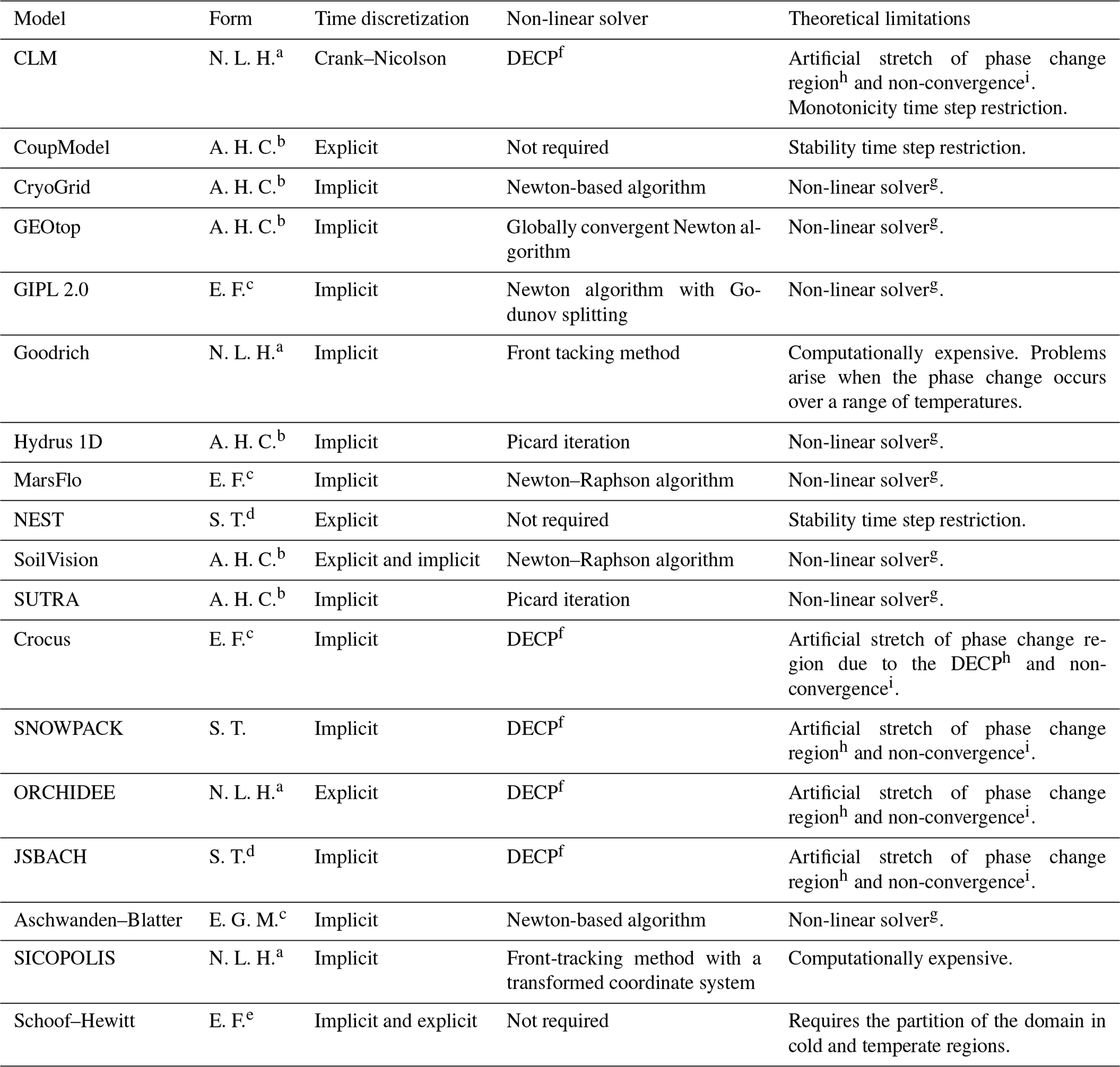
a The governing equation is written in only in terms of temperature and the latent heat is not included. b Apparent-heat-capacity formulation. c Enthalpy formulation. d Source term formulation. e The heat flux is written in terms of enthalpy and not of temperature as in the enthalpy formulation. f Decoupled energy conservation parametrization. g Convergence of the non-linear solver can be problematic (Casulli and Zanolli, 2010, 2012). h Nicolsky et al. (2007b). i Voller et al. (1990).
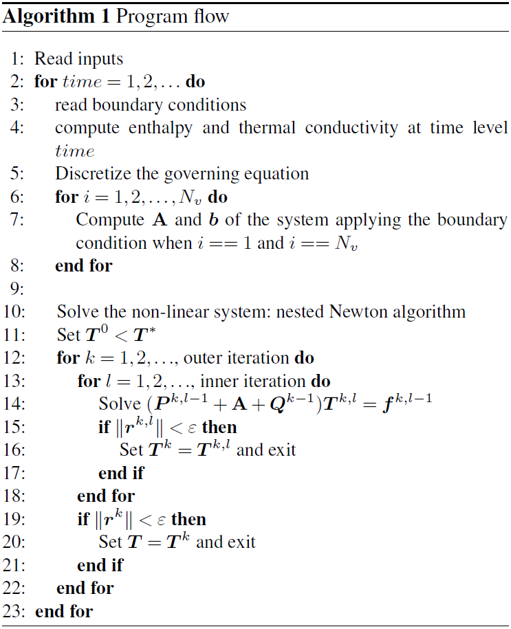
Frozen soil models are typically solved with time steps between seconds and hours. This may be motivated by the desire to resolve diurnal phenomena near the ground surface, and also this often arises from limitations of the numerical schemes used. Many applications related to permafrost (Teng et al., 2020), on the other hand, only require the representation of seasonal and multi-annual variation, which can be accomplished using time steps of 1 or more days if permitted by the numerical schemes employed. In order to have a numerical scheme that does not suffer from time step restriction due to a stability condition, an implicit time integration is required. An implicit formulation includes the necessity of solving a non-linear system of equations, and the algorithm used for this is of great importance. Existing linearization algorithms such as the Picard or the Newton algorithm require a sufficiently accurate initial guess. As reported by Casulli and Zanolli (2010, 2012) this can be obtained by using small time steps, often requiring an empirical criterion for time step adaptation. Therefore, even if the numerical scheme does not require a time step restriction, one may still be required to solve the non-linear system of equations. Because of this the convergence of Newton-type method is often problematic (Casulli and Zanolli, 2012). Instead, the NCZ algorithm always converges in any situation, even under the use of large time steps and grid sizes when the initial guess is chosen as suggested (Casulli and Zanolli, 2010, 2012). This is an important feature of the non-linear solver, because an inexact solution of the non-linear system is not conservative (Casulli and Zanolli, 2010).
3.1 Discretization of the domain
The domain is partitioned using an unstructured orthogonal grid (Casulli and Walters, 2000), consisting of a set of non-overlapping convex volumes Ωi, , separated by M internal faces Γj, . Let 𝒜j denote the non-zero jth face area. Within each control volume a centre must be identified in such a way that the segment joining the centres of two adjacent volumes and the face shared by the two volumes have a non-empty intersection, are orthogonal to each other, and have distance δj. Each control volume Ωi may have an arbitrary number of faces. Let ℱi denote the non-empty set of faces of the ith volume, with the exclusion of boundary faces. Moreover, let 𝒫(i,j) be the neighbour of volume i that shares face j with the ith control volume so that for all j∈ℱi. The discrete variables hi and Ti are located at centre of each element Ωi. Using an implicit finite-volume method, the discretization of Eq. (1) reads as
where Δt is the time step size,
and
is an optional source/sink term in volume, and hi(T) is the ith enthalpy given by
Equation (12) can be written in matrix form as
where T={Ti} is the vector of unknowns, h(T)=hi(Ti) is a vectorial function representing the discrete enthalpy, A is the energy flux matrix, and b is the right-hand-side vector of Eq. (12), which is properly augmented by the known Dirichlet boundary condition when necessary. For a given initial condition , at any time step Eq. (12) constitutes a non-linear system for , with the non-linearity affecting only the diagonal of the system and being represented by the enthalpy . This set of equations is a consistent and conservative discretization of Eq. (1). Therefore, regardless of the chosen spatial and temporal resolution, is a conservative approximation of the new temperature.
3.2 Solution of the non-linear system
Difficulties in solving the non-linear system of Eq. (16) arise from the non-monotonic behaviour of the derivative of the enthalpy, h(T), with respect to temperature, and because in some parametrizations used for substances, such as water, the derivative of the enthalpy is not correctly defined. The NCZ algorithm used here was discovered by Casulli and Zanolli (2010) and overcomes these difficulties applying the Newton algorithm in two subsequent iterations. NCZ is based on Jordan decomposition (Chistyakov, 1997) of the enthalpy function, rewriting it as the difference of two monotonic functions on which the Newton algorithm can be applied separately in a nested iteration, as explained below. A mathematical proof of convergence exists for NCZ (Brugnano and Casulli, 2008, 2009; Casulli and Zanolli, 2010, 2012).
For each control volume the enthalpy function hi(T) can be defined as
where Ca,i(T) is defined as . Ca,i(T) has to fulfil two requirements. The first one, C1, is that Ca,i(T) is defined for every T and that it is a non-negative function with bounded variations. The second one, C2, is that there exists a such that Ca,i(T) is strictly positive and non-decreasing in and non-increasing in .
Since Ca,i(T) are non-negative functions with bounded variations, they are differentiable almost everywhere, admit only discontinuities of the first kind, and can be expressed by using the Jordan decomposition (Fig. 1) as the difference of two non-negative, non-decreasing, and bounded functions:
Using Eq. (18) the enthalpy hi(T) can be written as , where
By making use of Eq. (19), the algebraic system, Eq. (16), can be written as
The NCZ algorithm requires first the linearization of h2 and then the linearization of h1. By choosing the initial guess for the NCZ algorithm such that , a sequence of outer iterates {Tk} is obtained from Eq. (20) by linearizing h2 as follows:
so that the outer iterates are solutions of the following non-linear system:
where and . The resulting kth (outer) residual is derived from Eq. (20) and reads as
For all , by setting , a sequence of inner iterates {Tk,l} is derived from Eq. (22) by linearizing h1(T) as
so that the inner iterates are determined from the following linear systems:
where and . The resulting (k,l)th (inner) residual is derived from Eq. (22) and reads as
The inner and the outer iterations are terminated when and , respectively, with ε being a sufficiently small pre-fixed tolerance.
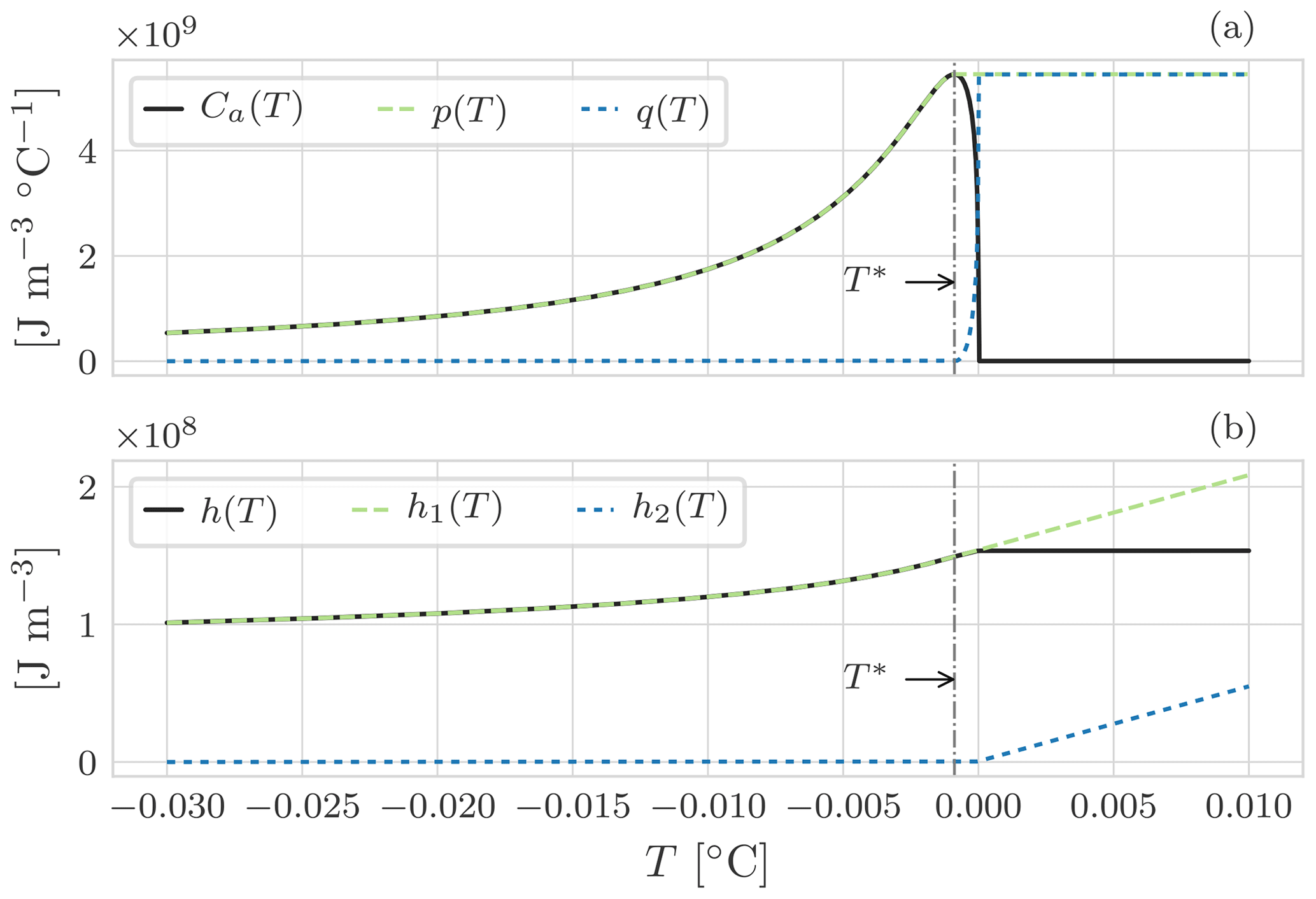
Figure 1Graphical representation of the Jordan decomposition for the enthalpy of soil using the SFCC model for a silty soil (Dall'Amico, 2010). Panel (a) shows the Jordan decomposition of Ca(T), Eq. (18). For , Ca(T) presents a maximum: for it is increasing, and for it is decreasing. This non-monotonic behaviour causes problems when solving the non-linear system. Ca(T) is thus replaced by p(T) and q(T), two monotonic functions. Consequently, in panel (b), h(T) is replaced by h1(T) and h2(T), Eq. (19).
The most commonly used constitutive SFCCs (McKenzie et al., 2007; Kozlowski, 2007; Dall'Amico et al., 2011; Sheshukov and Nieber, 2011; Watanabe et al., 2011), used to define the enthalpy of frozen soil, satisfy the assumptions C1 and C2. In particular, the NCZ approach can be successfully applied to SFCCs models derived from the combination of existing soil water retention curve (SWRC) models and the Clapeyron equation, which in general are difficult to implement in numerical models based on the apparent heat capacity (Kurylyk and Watanabe, 2013). Functions describing the internal energy of other substances, for instance pure water (Andreas, 2005), satisfy the assumptions C1 and C2, and, therefore, the NCZ method can be successfully used to model phase change problems as it will be shown for the original Stefan problem, Sect. 4.1.
The numerical model is compared for the problem of a column of freezing water, i.e. the Stefan problem, with the analytical solution presented by Neumann (cited in Kurylyk et al., 2014b), and for the problem of a column of soil with three zones – frozen, partially frozen, and unfrozen – with the analytical solution presented by Lunardini (1988).
4.1 Neumann analytical solution
The Neumann analytical solution gives the solution of unilateral freezing of a semi-infinite domain for both the temperature profile and the position of the moving boundary. Kurylyk et al. (2014b) recommended the Neumann solution due to its ability to represent differences between the thermal diffusivities of the thawed and frozen zones. Here we consider the freezing of pure water instead of soil since it is more numerically demanding. Consider a semi-infinite domain of pure water at temperature , where T0>Tm (Fig. 2). At the surface a Dirichlet boundary condition is imposed , with Ts<Tm. As a consequence a freezing front ζ propagates downward separating the solid and the liquid phase. The governing equations are
At the moving boundary ζ(t), the temperature is equal to the melting temperature of water, and the time evolution of ζ(t) is described by the third equation, the Stefan condition. This condition states that the difference of the heat fluxes at the interface of the two substances is consumed for the phase change.
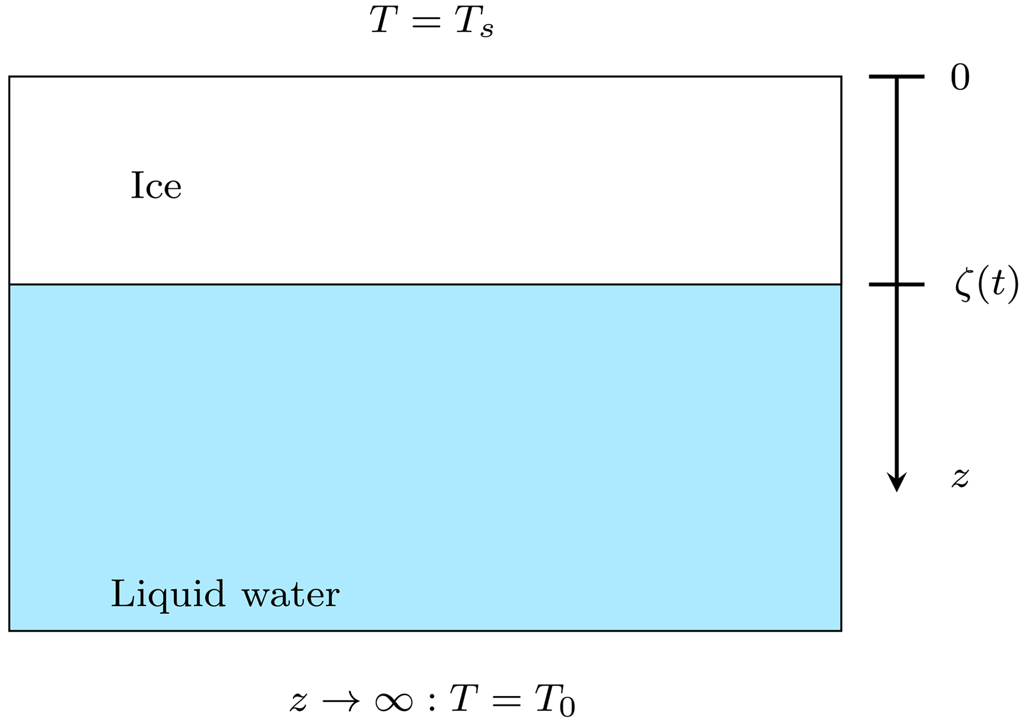
Figure 2Scheme showing the setting of the Neumann solution for the freezing case. Initially all water is liquid, T0>Tm. Because of the surface boundary condition, Ts<Tm, a freezing front, ζ, propagates downward.
The parameters used in the comparison are given in Table E1. The numerical model is able to simulate the freezing problem of water well as seen in Figs. 3 and 4.
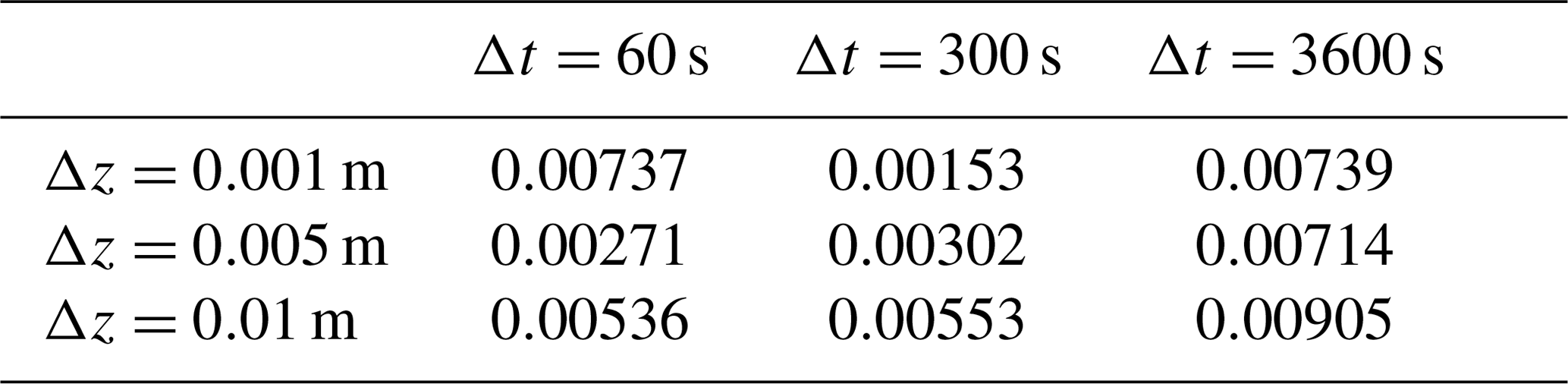
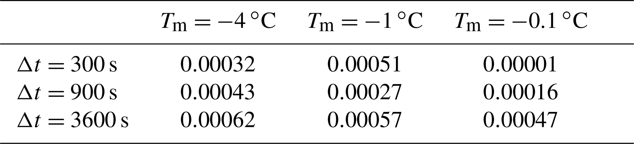
Table 2 Maximum error (m) of the freezing front position from the numerical solution with the NCZ algorithm for different space and time discretizations relative to the Neumann analytical solution. For the numerical solution the position of the freezing front has been reconstructed from the linear interpolation of the temperature profile.
For comparison, Kurylyk et al. (2014b) tested the numerical model SUTRA against the Neumann analytical solution considering a soil porosity of 0.50 m3 m−3. For their test the time step was of 0.04–0.4 s, the vertical spatial discretization was 0.001 m, and the parameter ϵ was increased to −0.01 ∘C to match the analytical solution. The maximum absolute error of the freezing front position was 0.00099 m.
In our model, the choice of a small melting temperature range ϵ=0.0001 ∘C does not affect the quality of the numerical solution even at a large time step of 3600 s. Looking at Table 2 it is clear that the choice of the time step size is somehow related to the choice of the spatial discretization: using a small time step with a coarse grid does not necessarily improve the accuracy of the position of the freezing front.
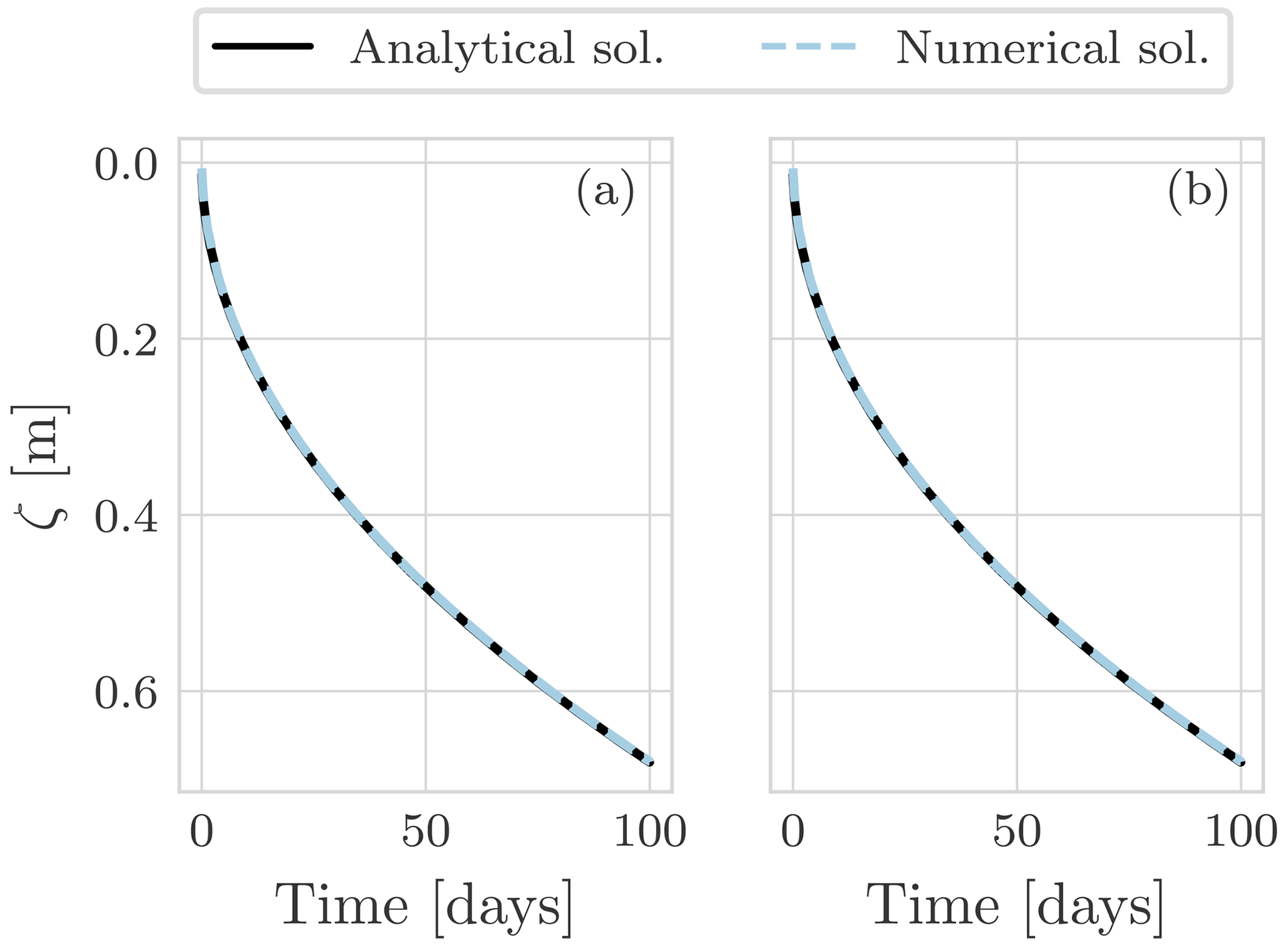
Figure 3Propagation of the freezing front compared between the Neumann analytical and the numerical solution with the NCZ algorithm. Two space discretizations are used: (a) Δz=0.005 m and (b) Δz=0.001 m. The integration time step is Δt=3600 s.
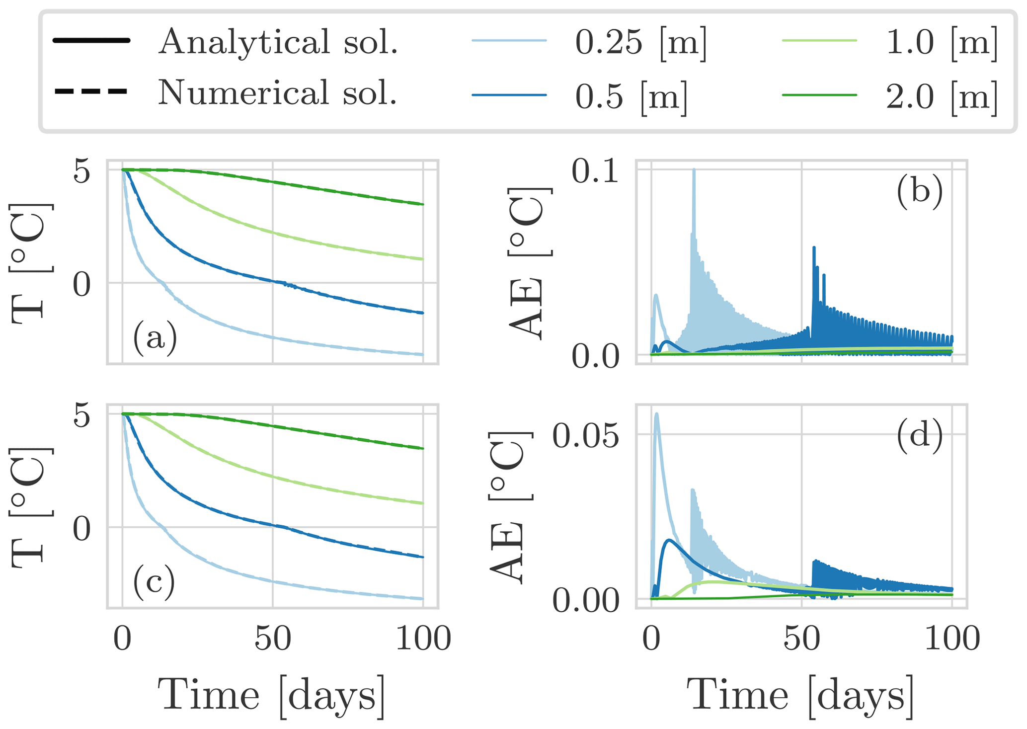
Figure 4Panels (a) and (c) show the temperature evolution for the Neumann analytical and the numerical solution with the NCZ algorithm at various depths for a spatial discretization Δz=0.005 m and Δz=0.001 m respectively. The integration time step is Δt=3600 s. Panels (b) and (d) show the absolute error.
We use the Neumann analytical solution to assess the robustness of the NCZ algorithm in comparison with the Newton–Raphson and globally convergent Newton methods. As reported by Dall'Amico et al. (2011), Fig. 5 represents a well known case for which the Newton–Raphson algorithm cannot converge. Instead, the solution continuously cycles between the iterates Tk−1 and Tk.
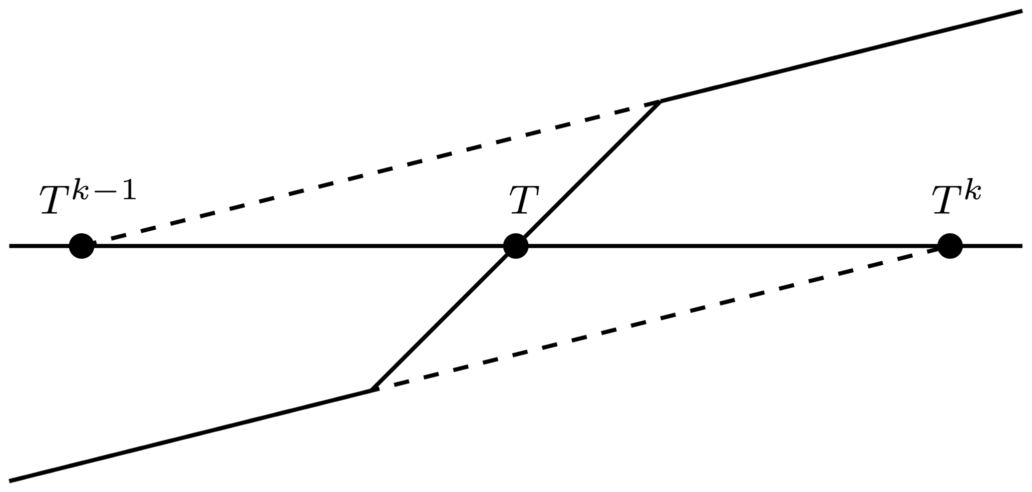
Figure 5A scheme of the problem which illustrates how the Newton–Raphson method cannot converge towards T (Dall'Amico, 2010). In this case, the Newton–Raphson method fails to converge to T since it cycles between Tk and Tk+1 values.
While the Newton–Raphson algorithm converges to the exact solution if a good initial guess for Tk exists, this represents a severe constraint for the reliable application for an iterative algorithm in a numerical model. An improvement of the Newton–Raphson algorithm can be obtained using the globally convergent Newton scheme (Dall'Amico et al., 2011). It uses the Newton–Raphson algorithm to provide the right search direction, and, in order to avoid overshooting, a reduction factor δ is used to find the new estimate. This represents an improvement over the Newton–Raphson method, but its ability to converge depends on the choice of the parameter δ and on the treatment of the apparent heat capacity (Hansson et al., 2004; Nicolsky et al., 2007b; Dall'Amico et al., 2011). Moreover, the Newton–Raphson and the globally convergent Newton methods do not guarantee convergence for any time step size, and this represents a limiting factor whenever reaching the convergence is necessary to reduce the time step size. For example, in (Dall'Amico et al., 2011) the comparison between the Neumann solution and GEOtop has been done with a time step of 10 s.
A comparison of the numerical solutions obtained with the Newton–Raphson algorithm, the globally convergent Newton algorithm, and the NCZ algorithm shows significant differences (Fig. 6). Newton–Raphson cannot reproduce the analytical solution even if a time step of Δt=10 s is used. The globally convergent Newton is in good agreement with the analytical solution if Δt=10 s. With an hourly time step, however, the example with the globally convergent Newton method is not able to reproduce the position of the freezing front over longer periods of time. By contrast, the NCZ algorithm reproduces the analytical solution well using Δt=3600 s.
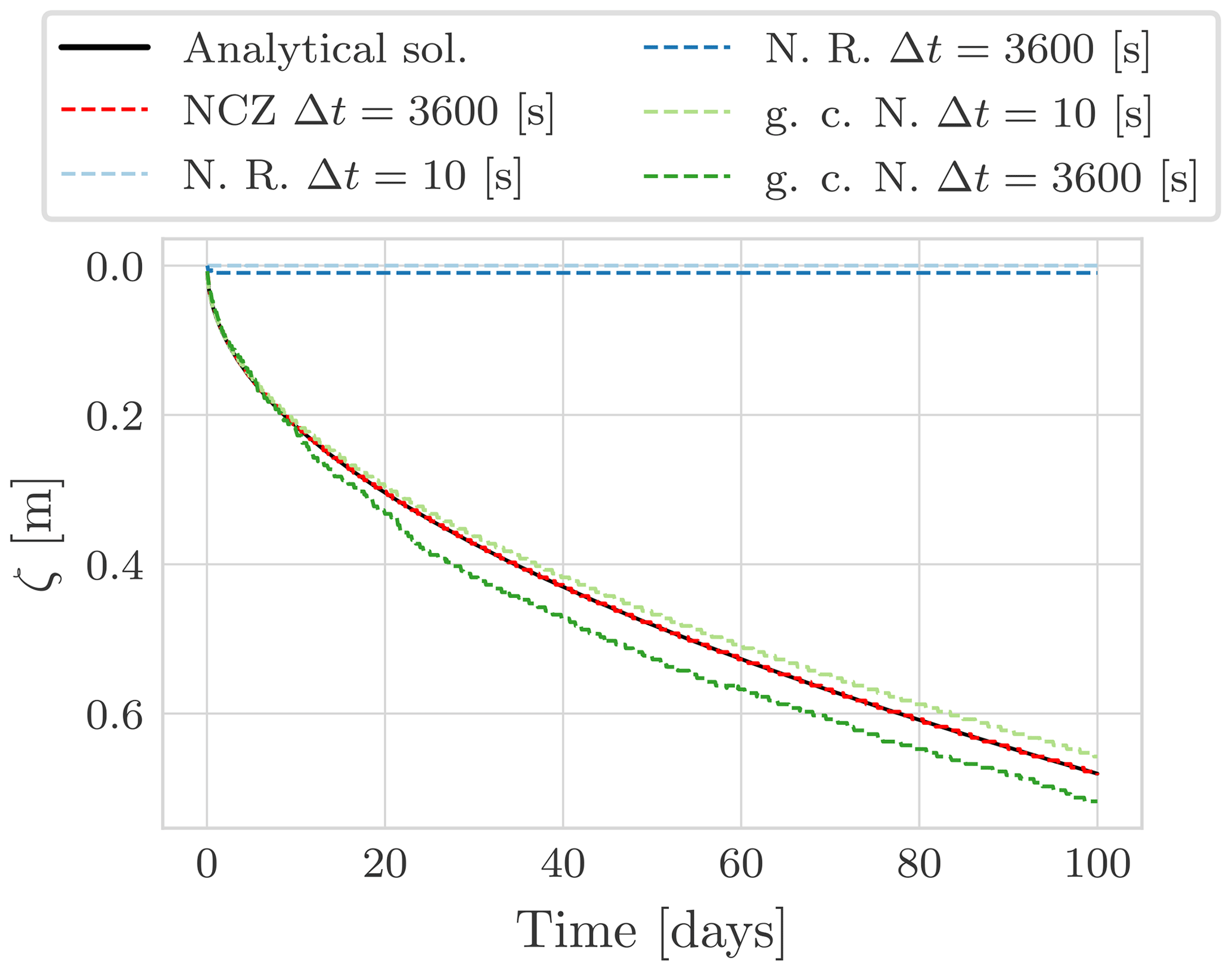
Figure 6Comparison between the Neumann analytical solution and the numerical solution obtained with the Newton–Raphson (N. R.), globally convergent Newton (g. c. N.), and NCZ algorithms. All the numerical simulations use the same spatial discretization Δz=0.005 m.
The quality of the solution obtained with the globally convergent Newton algorithm depends not only on the time step duration but also on the definition of the parameter δ (Fig. 7). The additional necessity for an arbitrarily chosen parameter in the globally convergent Newton algorithm further underscores the robustness of the NCZ algorithm, for which convergence only depends on the right definition of Eqs. (18) and (19).
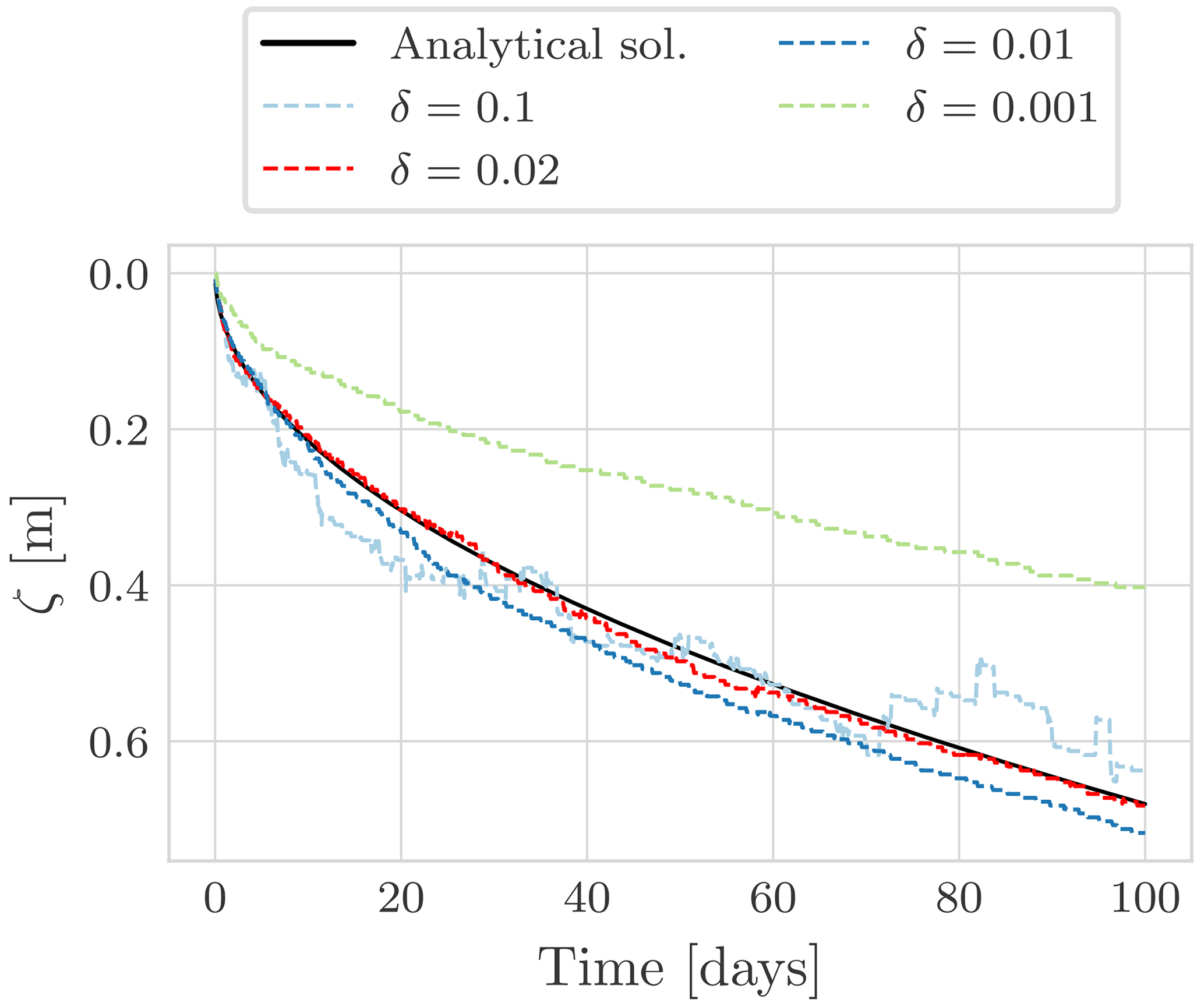
Figure 7Comparison between the Neumann analytical solution and the numerical solution obtained with the globally convergent Newton algorithm (g. c. N.). All the numerical simulations use the same spatial discretization Δz=0.005 m and a time step size of Δt=3600 s. This figure shows as the numerical solution depends on the choice of the parameter δ.
4.2 Lunardini analytical solution
Lunardini (1988) derived an analytical solution (Appendix F) for the temporal evolution of temperature during the freezing of a semi-infinite and initially unfrozen soil column. In contrast to the Neumann analytical solution, in the Lunardini analytical solution the domain is divided into three regions (Fig. 8) on the basis of temperature: unfrozen, T<Tm; partially frozen, ; and fully frozen, T>Tf. The domain is initially unfrozen with ∘C. At the left boundary condition a Dirichlet boundary condition is imposed with ∘C, and the right boundary temperature is kept equal to the initial condition, . Because the left boundary condition Ts<0 ∘C, a freezing front propagates from left to right.
We computed benchmark T1 proposed by the InterFrost project (, ); parameters are given in Table F1. The model agrees well with the analytical solution for all the three cases of Tm in terms of both the temperature profile, Fig. 9 and Table 3, and the freezing front position, Fig. 10 and Table 4, even with an hourly time step.
For comparison, McKenzie et al. (2007) compared the numerical model SUTRA against the Lunardini analytical solution for the cases ∘C and ∘C using a time step size of 900 s and a space resolution of 0.01 m. For the first test case the maximum absolute error was 0.01 ∘C, and for the second test case it was 0.1 ∘C. Their parameters, however, differ from those suggested by the InterFrost consortium, making performance comparisons difficult. In particular, their porosity was 0.05 m3 m−3, whereas InterFrost uses 0.336 m3 m−3. As this determines the amount of latent heat involved in phase change, smaller errors are suspected to occur with the parameters used by McKenzie et al. (2007).
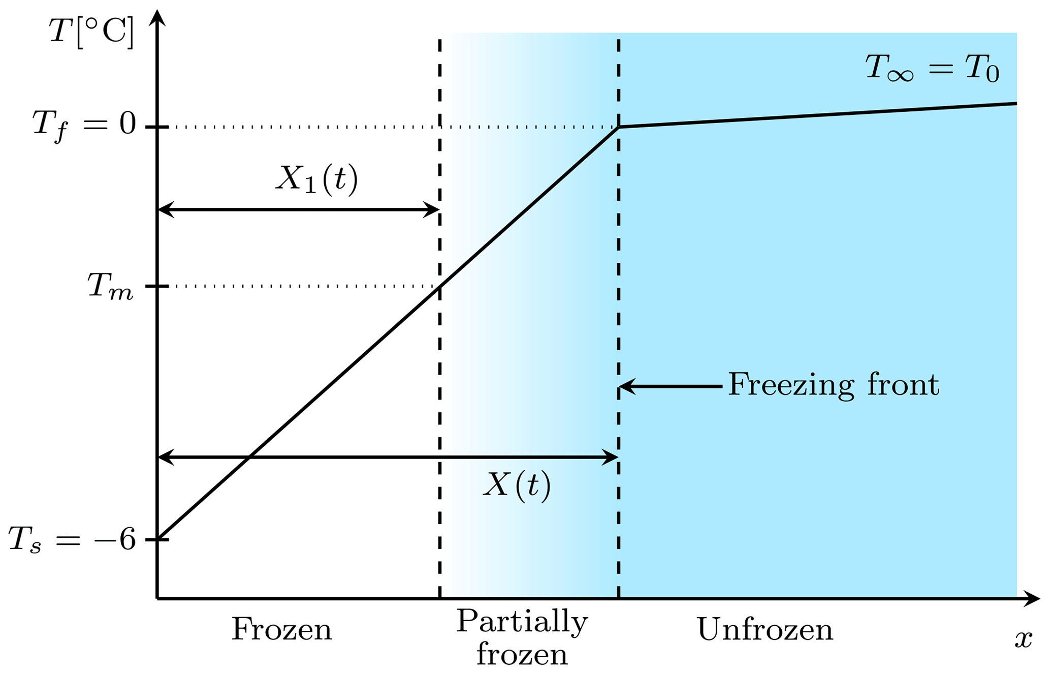
Figure 8Scheme showing the setting of the Lunardini problem (Ruhaak et al., 2015). Initially the domain is unfrozen with T=T0. Because of Ts<0 on the left boundary, a freezing front propagates from left to right. X1(t) and X(t) identify respectively the isotherm corresponding to Tm and Tf.
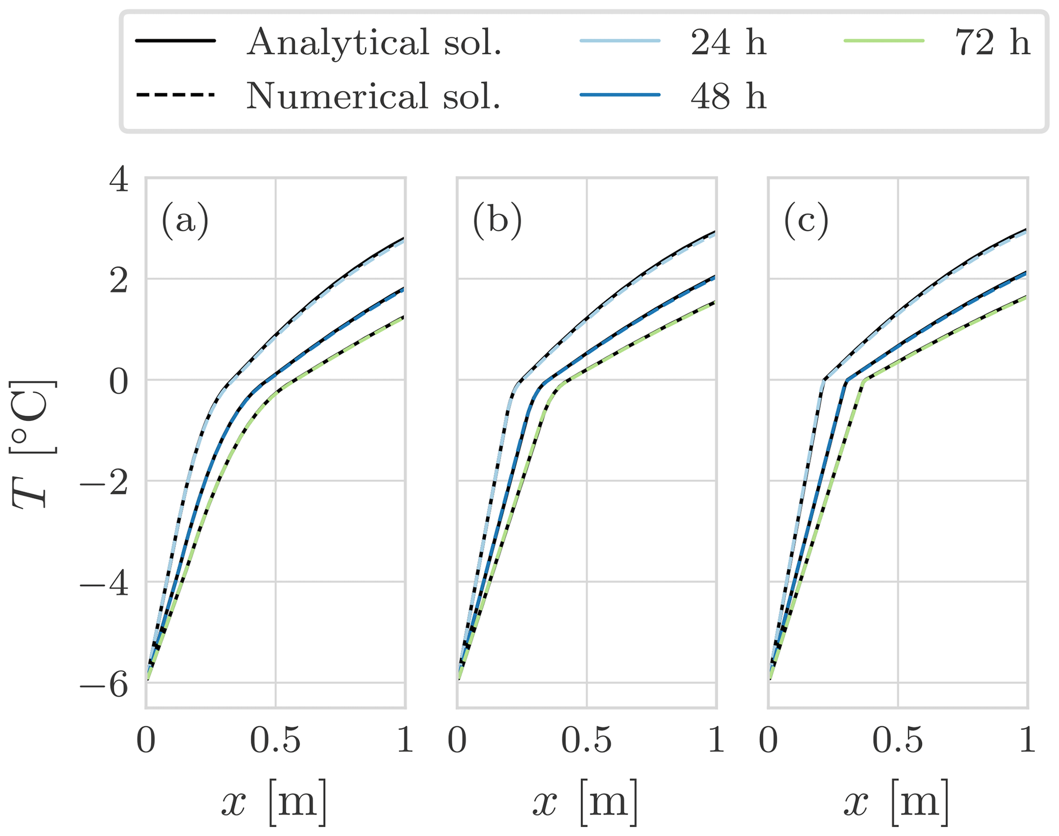
Figure 9Comparison between the Lunardini solution and the numerical solution with the NCZ algorithm for the three cases of the T1 benchmark: (a) ∘C, (b) ∘C, and (c) ∘C. The colours represent different time frames. The integration time step is Δt=3600 s, and the space resolution is Δx=0.01 m.
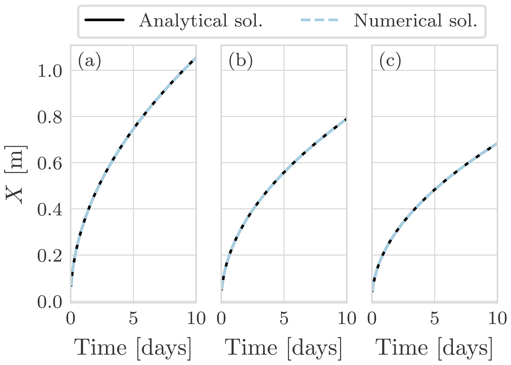
Figure 10Propagation of the zero isotherm for the Lunardini solution and the numerical solution with the NCZ algorithm for the three cases of T1 benchmark: (a) ∘C, (b) ∘C, and (c) ∘C. The integration time step is Δt=3600 s, and the space resolution is Δx=0.01 m.
Table 3Maximum absolute error ∘C of the temperature after 24 h from the numerical solution with the NCZ algorithm relative to the Lunardini analytical solution. The space resolution is Δx=0.01 m.

Table 4Maximum error (m) of the freezing front position from the numerical solution with the NCZ algorithm relative to the Lunardini analytical solution. The space resolution is Δx=0.01 m.
In the previous sections, we have demonstrated that the proposed method can reproduce the Neumann analytical solution, as well as the Lunardini analytical solution, even when using larger time steps than other numerical models.
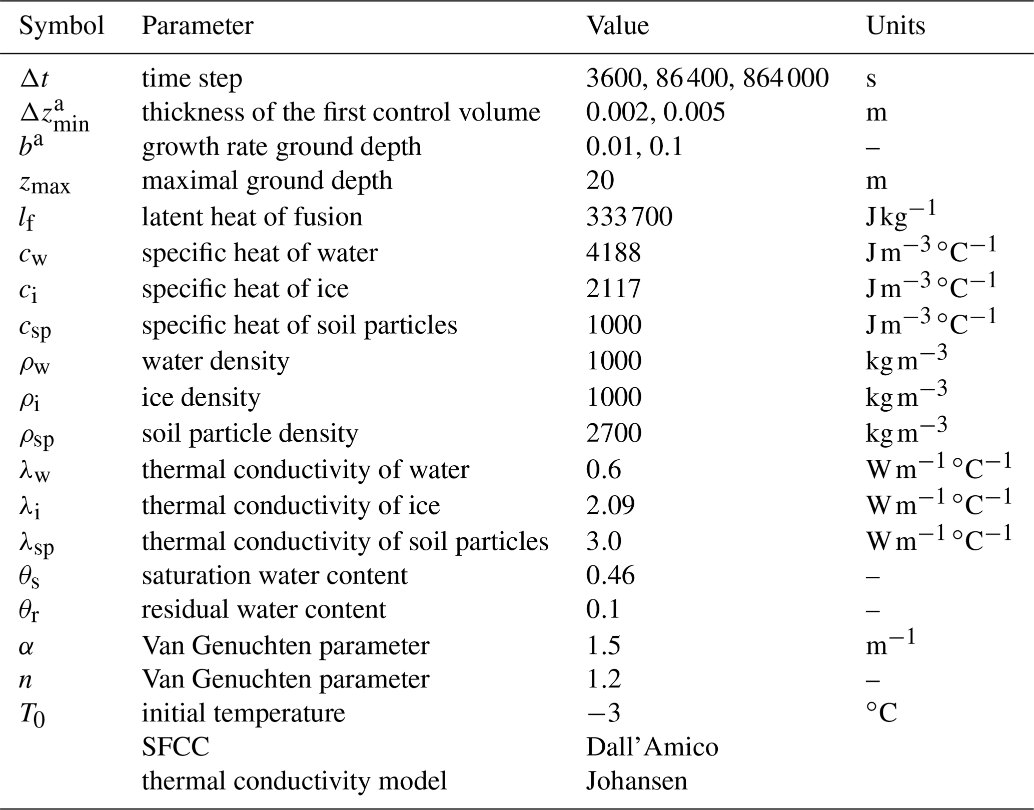
After comparing simulation results with analytical solutions, we now analyse the difference between solutions using hourly, daily, and 10 d time steps. The domain is a soil column of 20 m depth that is uniformly at ∘C, initially. The bottom boundary condition is adiabatic, and at the surface we use a Dirichlet boundary condition. The original forcing has hourly resolution, and for longer time steps corresponding averages are computed. As temperature gradients and the influence of phase change are usually greatest near the soil surface, the thickness Δz is parametrized with an exponential function (Gubler et al., 2013):
where Δzmin is the thickness of the first layer, b is the growth rate, and i is the layer index, being one at the ground surface and increasing downward. The parameters used are reported in Table G1. All three simulations were spun up for a period of 1400 years to reach a stable thermal regime. After spin-up, we performed a simulation of 100 years.
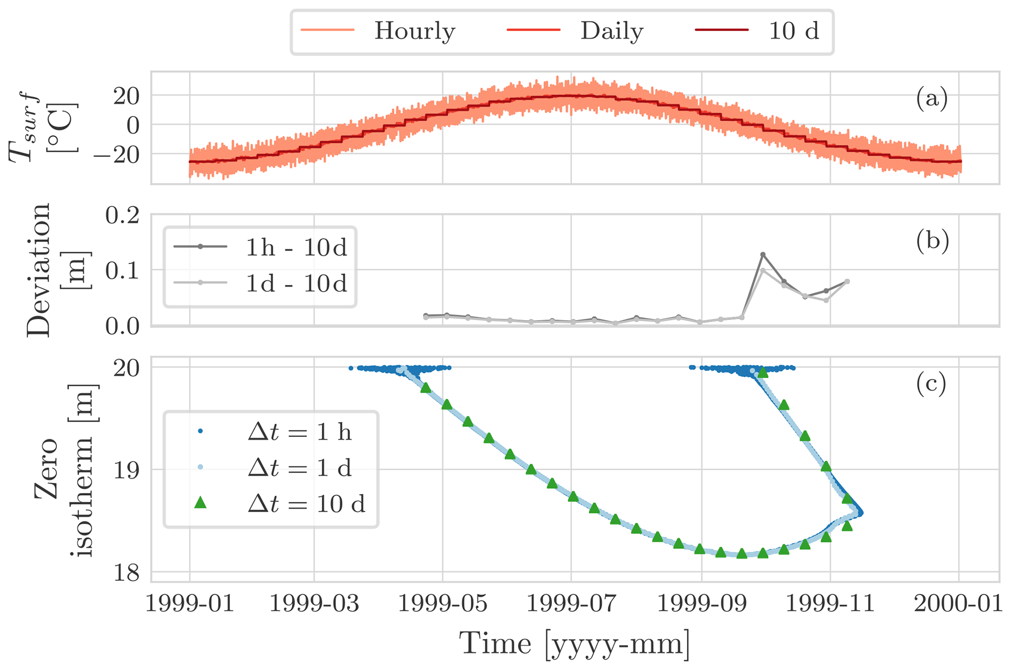
Figure 11Comparison of the position of the zero isotherm, panel (c), after 100 years of three simulations: using an hourly boundary condition with time step of Δt=1 h, using a daily boundary condition with a time step of Δt=1 d, and using a 10 d boundary condition with a time step of Δt=10 d. Panel (a) shows the surface temperature for the hourly, the daily, and the 10 d simulations. Panel (b) shows the deviation of the position of the zero isotherm after 100 years between the hourly and the 10 d simulation, as well as between the daily and the 10 d simulation.
Figure 11 compares the zero-isotherm position computed after 100 years for the three different time steps. Interestingly, there are no significant deviations in the results. The larger deviations occur when the zero isotherm is shallow: at the beginning of the thawing season as well as the freezing one (Figs. G1 and G2). These differences can be explained by the different surface temperature used to drive the simulations (see Appendix G) and by the fact that in using a larger time step we lose accuracy in the numerical solution.
With larger time steps, we lose some of the information of the boundary conditions, and the accuracy of the numerical model decreases because it is first-order accurate in time. The overall performance relative to simulations with smaller time steps, however, is largely preserved. While the order of accuracy can be increased to second order in time using the Crank–Nicolson method, this would incur a time step restriction to guarantee the monotonicity of the solution. As this restriction is proportional to the square of the space discretization, Δz2, the Crank–Nicolson method would represent a severe constrain whenever high spatial resolution is required.

Figure 12(a) The minimum, mean, and maximum temperature profile for the hourly simulation. Panels (b), (c), and (d) show the comparison of the minimum, mean, and maximum temperature profile respectively for the three simulations: with an hourly air temperature boundary condition and Δt=1 h, with a daily air temperature boundary condition and Δt=1 d, and with a 10 d air temperature boundary condition and Δt=10 d. All three simulations last 100 years. The maximum difference of Tmean between the hourly and daily simulation is 0.04 ∘C, while between the hourly and 10 d simulation the difference is 0.3 ∘C.
Figure 12 compares the minimum, mean, and maximum temperature profile respectively for the three simulations. Panel (a) shows the ground temperature envelope for the hourly simulation. The maximum envelop presents an “elbow” that is due to the zero-curtain effect Fig. G3. As can be seen in panels (b) and (d), close to the soil surface the hourly simulation presents larger values for both the minimum and maximum temperature due the fact that the hourly boundary condition presents a greater amplitude that is smoothed computing the daily and 10 d average.
In the mean temperature profile, the 10 d simulation presents a larger deviation from the hourly simulation than the daily simulation. The large deviation can be explained with the interaction of the time step size with the thermal offset effect (Fig. G4). If the thermal conductivity of water is set equal to that of ice, the maximum difference between the three profiles is reduced to 0.003 ∘C with a maximum deviation of 0.003 ∘C from the initial condition, which is also equal to the mean of the forcing boundary condition.
So far we have compared the results of the model with the choice of the time step size; in Appendix G we compare with the choice of the spatial discretization. The results are still in good agreement, but it is interesting to note that the zero isotherm presents some steps, independently of the size of the time step, and some details are missed, such as the joining of the downward and upward freezing fronts captured with the finer grid. These steps are caused by the greater thickness of the grid elements. Because temperature is computed in the middle of each control volume, more time is required to achieve complete phase change of water, resulting in slower variation of the zero-isotherm position.
These synthetic experiments demonstrate that spatial and temporal discretization can be chosen accordingly to the aim the study without any constrains due to the convergence and stability issues of the numerical scheme.
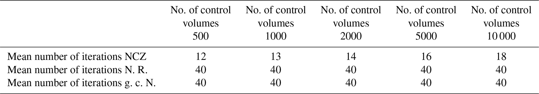
Moreover, we checked the mean number of iterations required to solve the non-linear system for a simulation lasting 1 year with a time step Δt=1 h and for different spatial discretizations. We compared the NCZ against the Newton–Raphson algorithm and the globally convergent Newton. Results are reported in Table G2.
We have presented a new model for simulating the ground thermal regime in the presence of freezing and thawing based on the heat-transfer equation and the application of the NCZ algorithm. To our knowledge, this is the only method that guarantees convergence while also permitting large time steps. The numerical model was implemented and verified against the Neumann and Lunardini analytical solutions. In both cases, the results were in good agreement even with an hourly integration time step. For the Neumann solution, we considered pure water instead of saturated soil since it is more numerically demanding, and no convergence problems were encountered despite choosing a narrow temperature range (0.0001 ∘C) over which phase change occurs.
Numerical experiments demonstrated the robustness of the model by comparing results at differing temporal and spatial resolutions. Results obtained with time steps of 1 h, 1 d, and 10 d are consistent. The robustness of the numerics allows the user to choose both the space and time discretization without any restriction due to stability and convergence issues. As a consequence, this method is effective for simulating permafrost thaw, a phenomenon that occurs at depth, in response to seasonal and multi-annual cycles, and often over tens, hundreds, or even thousands of years. Furthermore, phenomena like hysteresis or the variation of solute concentration upon freezing (Clow, 2018) can be included in the numerical model if the enthalpy function (i.e. its parameters) does not change within the current time step of integration.
While we presented a finite-volume method, the NCZ algorithm can be also used with the finite-difference and finite-element method. Beyond applications to frozen soil, it can be used to study other geophysical phenomena that involve phase change of a substance simply by changing the definition of the enthalpy function and the thermal conductivity function. Examples include glacier dynamics (Aschwanden et al., 2012), snowpack evolution (Brun et al., 1992; Lehning et al., 1999), and magma bodies (De Lorenzo et al., 2006). This may be even further expanded to industrial problems involving phase change materials used in energy recovery systems (Mongibello et al., 2018; Nazzi Ehms et al., 2019) or casting problems of pure metals and alloys (Lewis and Ravindran, 2000).
The heat equation can be written in different forms that are analytically equivalent but subject to differing numerical advantages and disadvantages. In the scientific literature, several simulators, i.e. software that implements a particular model (set of equations), for solving the heat equation with freezing and thawing have been presented. Here we review commonly used frozen soil models in terms of their governing equations and methods of finding numerical solutions.
Heat transfer with phase change of water is a cross-cutting problem existing in many geophysical phenomena other than frozen soil. This includes, for example, the seasonal snowpack, glaciers, and ice sheets. Our contribution does not seek to present an improvement in the description of these problems, and we ignore typical processes such as metamorphism and settling in seasonal snow or strain heating and deformation in glaciers and ice sheets. Nevertheless, corresponding models may benefit from the NCZ algorithm in the treatment of the non-linearity arising from phase change, and, furthermore, broadening our review to also include some snow and glacier models supports the generalization of our findings.
A1 CLM
The Community Land Model (CLM) is the LSM for the Community Earth System Model (Oleson et al., 2004). It includes a module to simulate the ground temperature considering freezing and thawing. The governing equation is written in the non-conservative form and does not include the latent heat term (Oleson et al., 2004; Lawrence et al., 2019). The heat conduction equation is solved using a Crank–Nicolson method. The temperature profile is calculated by adopting the DECP approach. This approach does not require solving a non-linear system, since the latent heat is treated in an explicit way, but Nicolsky et al. (2007a) have pointed out that this two-step procedure can overestimate the region where the phase change occurs, resulting in inaccuracies in the simulation of active-layer thickness.
A2 CoupModel
The CoupModel (Jansson and Karlberg, 2011) is a one-dimensional numerical model to simulate the heat and water flow as well as carbon and nitrogen budgets in a soil–plant–atmosphere system (Hollesen et al., 2011). The governing equation for heat flow in the soil is defined using the apparent heat capacity and solved with an explicit numerical method. This does not require solving a non-linear system but sets a time step restriction to avoid numerical oscillation.
A3 CryoGrid
CryoGrid 2 simulates the ground thermal regime based on conductive heat transfer in the soil and in the snowpack (Westermann et al., 2013). The heat equation is written using the apparent heat capacity and solved using the method of lines (Westermann et al., 2013). The resulting system of ordinary differential equations is solved numerically with the package CVODE of Sundials that implements a modified Newton method, and an inexact Newton method, or a fixed-point solver to linearize the algebraic system resulting from the discretization of the heat-transfer equation. The convergence of the Newton-type methods can be problematic (Casulli and Zanolli, 2012).
A4 GEOtop
GEOtop (Rigon et al., 2006; Endrizzi et al., 2014) is a physically based distributed model of the mass and energy balance of the hydrological cycle. It includes a module for solving the energy equation in freezing soil (Dall'Amico et al., 2011); this module can also be linked with the solver for the Richards equation. The governing equation for heat transfer is written in conservative form, but when solving the equation the apparent-heat-capacity formulation is used. A globally convergent Newton algorithm is used to deal with the non-linearities arising from phase change (Dall'Amico et al., 2011). The globally convergent Newton algorithm represents an improvement over the Newton–Raphson algorithm; however, as shown in Sect. 4.1 it does not perform as well as the NCZ algorithm, and additionally the choice of the parameter δ is non-trivial.
A5 GIPL 2.0
GIPL 2.0 simulates the ground thermal regime by solving the heat equation with phase change numerically (Marchenko et al., 2008). The governing equation is written in the conservative form, and Newton's method is used to linearize the energy equation. To overcome convergence problems when solving the non-linear system, GIPL 2.0 implements a fractional time step approach – Godunov splitting. The key point of the solution regards the treatment of the enthalpy time derivative: if a non-zero gradient of temperature exists, the time derivative is approximated with a difference derivative; otherwise, it is approximated using the analytical representation.
A6 Goodrich
Goodrich (1982) presented a one-dimensional model to simulate the ground thermal regime considering the phase change of water. The governing equation is written in the non-conservative form and does not include the latent heat of fusion. Phase change is treated with the front-tracking method, which offers good accuracy for problems in which phase change occurs at a fixed temperature (Goodrich, 1982). This model does not use a SFCC, and instead the soil is represented as homogeneous layers with distinct frozen and thawed thermal properties.
A7 Hydrus 1D
Hydrus 1D includes a module to simulate water flow and heat transport in frozen soil. The governing equation is written using the apparent-heat-capacity formulation, and the Picard iteration is used to linearize the algebraic non-linear system. In their paper, Hansson et al. (2004) explain that during the Picard iteration the solution can easily oscillate whenever the temperature decreases below the melting temperature. To avoid these oscillation the temperature is reset to the critical value and the iteration restarted. Hydrus 1D adopts an empirical time step adaptation criterion. It is worthwhile to note that the modified Picard iteration was proposed by Celia et al. (1990) to solve the Richards equation – a problem for which the NCZ algorithm was originally proposed (Casulli and Zanolli, 2010).
A8 MarsFlo
MarsFlo is a three-phase numerical model to simulate the heat transfer and water flow in partially frozen, partially saturated porous media (Painter, 2011). The heat equation is written in the conservative form. The equation is solved using an implicit finite-difference method, and the resulting non-linear system is solved using a Newton–Raphson method. To overcome convergence and stability problems, three modifications were introduced (Painter, 2011). The convergence of the Newton–Raphson method can be problematic (Casulli and Zanolli, 2012).
A9 NEST
Zhang et al. (2003) developed the one-dimensional physically based Northern Ecosystem Soil Temperature (NEST) model. The heat equation is written in the source term formulation and solved with the DECP approach. The numerical method is explicit in time; thus the maximum time step is 30 min to prevent oscillations in the solution.
A10 Sergueev et al.
This is a two-dimensional model, and the governing equation is written in the enthalpy form (Sergueev et al., 2003). This model implements a fractional time step approach (Godunov splitting): each time step is divided into two steps, and at each step a different dimension is treated implicitly. The system of finite-difference equations is non-linear and is solved with Newton's method. As in GIPL 2.0, the time derivative of enthalpy is computed using either the difference derivative or the analytical derivative according with the gradient of the temperature field.
A11 SoilVision
The heat equation is written using the apparent heat capacity. The equations are solved using a finite-element solver, FlexPDE suite, both explicit and implicit in time. In the case of implicit methods, the resulting non-linear system is solved using the Newton–Raphson method. The convergence of the Newton–Raphson method can be problematic (Casulli and Zanolli, 2012).
A12 SUTRA
SUTRA is an established USGS groundwater flow and coupled transport model (Voss and Provost, 2002). McKenzie et al. (2007) and McKenzie and Voss (2013) have extended the model to simulate freezing and thawing processes in the soil. The heat equation is written using the apparent-heat-capacity formulation, and non-linearities are solved using the Picard iteration. The convergence of the Newton-type method can be problematic (Casulli and Zanolli, 2012).
A13 Crocus
Crocus is a one-dimensional finite-difference model that solves the mass and energy balance within the snowpack taking into account metamorphism and settling. The first versions of Crocus (Brun et al., 1989, 1992) were not enthalpy-based. The governing equation was written in terms of temperature and water content. It was solved by using the Crank–Nicolson method, and the phase change is treated by using the DECP approach (Brun et al., 1992). After the integration within SURFEX (Vionnet et al., 2012), Crocus uses the enthalpy formulation, and the numerical scheme is fully implicit, based on the numerics of ISBA-ES (Boone and Etchevers, 2001). Similarly to the previous version, the heat balance equation is solved by adopting the DECP approach (Boone and Etchevers, 2001). Even though recent work Crocus is based on a simple bucket approach for liquid water percolation (Morin et al., 2012; Lafaysse et al., 2017), D'Amboise et al. (2017) implemented a routine for water flow in the snowpack based on the Richards equation, which is characterized by non-linear behaviour like the enthalpy equation. To solve it, they adopted an approach based on the Picard iteration with variable time steps (Paniconi and Putti, 1994).
A14 SNOWPACK
SNOWPACK (Lehning et al., 1999) solves the heat transfer and creep/settlement equations using a Lagrangian finite-element method. The governing equation is written using the source/sink formulation, and it is solved using the DECP approach (Bartelt and Lehning, 2002; Lehning et al., 1999). Regarding the water flow, SNOWPACK implements three different schemes: a simple bucket-type approach, an approximation of the Richards equation, and the full Richards equation (Wever et al., 2014). The full Richards equation is solved using the Picard iteration with variable time steps (Paniconi and Putti, 1994).
A15 ORCHIDEE
ORCHIDEE is terrestrial biosphere model, and it is part of the IPSL-CM4 Earth system model developed by the Institut Pierre Simon Laplace (IPLS) (Krinner et al., 2005). In the version 1.9.6 the snow is described with a single layer of constant density (Wang et al., 2013). Because of the limitations of the this approach, Wang et al. introduce a three-layer snow model, ORCHIDEE-ES, largely inspired from ISBA-ES (Boone and Etchevers, 2001) to consider snow settling, water percolation, and water refreezing. The governing equation is written in the non-conservative form and does not include the latent heat term. The temperature profile is calculated by adopting the DECP approach.
A16 JSBACH
JSBACH is the land-surface model developed by the Max Plank Institute (Ekici et al., 2014). It is a component of the Max Planck Institute Earth system model (MPI-ESM) that also includes ECHAM6 for the atmosphere and the Max Planck Institute ocean model (MPI-OM) for the ocean. JSBACH simulates both the frozen soil and the snowpack. In both cases the heat conduction is assumed to be the dominant method of heat transfer. The governing equation is written in the source term formulation and solved with the DECP approach (Ekici et al., 2014).
A17 Ice-sheet models
For glacier and ice-sheet models it is necessary to distinguish between cold and temperate ice. Following Aschwanden and Blatter (2005), “ice is treated as temperate if a change in heat content leads to a change in liquid water content alone, and is considered cold if a change in heat content leads to a temperature change alone”. This means that cold ice is always below the melting temperature and thus the phase change does not occur. As result, present-day ice-sheet models can be classified into cold-ice method models and polythermal models.
The cold-ice method does not consider the phase change of ice. Because of this the heat capacity can be assumed to be constant, and therefore the governing equation can be written in terms of only temperature. These models are easy to implement, but their applicability is restricted since in general temperate zones can be present (Aschwanden and Blatter, 2009). In fact, since the phase change of ice is overlooked; locally, the cold-ice method violates the energy conservation, overestimates the temperate region (Aschwanden and Blatter, 2009), and cannot quantify the liquid water content that affects viscosity in temperate ice (Lliboutry and Duval, 1985).
By contrast, polythermal ice-sheet models consider the phase change of ice. Similar to freezing soil models, the polythermal ice-sheet models can be classified in two groups on the base of the treatment of the phase change: front-tracking method and enthalpy method (Nedjar, 2002). SICOPOLIS (Greve, 1997a, b; Greve and Blatter, 2016) is the only truly polythermal ice-sheet model. It employs the polythermal two-layer scheme (Greve, 1997b): the temperature field and the water content field are computed separately for the ice and temperate domain, and a Stefan-type condition is applied at the cold-temperate surface (CTS). This model defines the CTS for both energy flux and mass flux. The drawback of this method relates to the implementation and restriction on the geometry and topology of the CTS (Aschwanden et al., 2012).
Aschwanden and Blatter (2009) presented an enthalpy gradient method. This is a fixed-grid method that differs from the enthalpy method commonly used for freezing soil in its definition of the energy flux. In the enthalpy method, the heat flux is expressed in terms of the temperature gradient, whereas in the enthalpy gradient method it is expressed in terms of enthalpy, assuming that the heat capacity is constant (Aschwanden and Blatter, 2009). The enthalpy approach combines the advantage of solving one equation for the entire domain, cold-ice models, and the correct description of the thermodynamics of temperate ice (front-tracking model). This model is implemented in COMSOL Multiphysics (Aschwanden and Blatter, 2009), where non-linear problems are solved using either a Newton algorithm or a damped Newton algorithm. Also in this case the NCZ may represent a valid option to solve the non-linear system. To the authors' knowledge, the enthalpy gradient method has not be used in freezing soil models.
Hewitt and Schoof (2016) presented an enthalpy-based finite-volume method for polythermal ice. To solve the equation at each time step the computational domain is explicitly divided in the cold and temperate regions, and the energy equation is solved by adopting a combination of implicit and explicit methods (Hewitt and Schoof, 2016). It is worth noting that in the temperate region, temperature is set equal to the melting temperature of the ice. This limits the application of this model to simulate freezing soil, where temperature can be higher than the melting temperature of water.
We present the pseudocode for a one-dimensional implementation of the NCZ algorithm. Since the matrix A in Eq. (16) is tri-diagonal, we can efficiently compute only the non-zero diagonal: the upper diagonal, the main diagonal, and the lower diagonal. We use the generic expression Discretize the governing equation since here we can choose to adopt either a finite-volume method, as presented in this paper, a finite-element method, or a finite-difference method. Moreover, the matrix A is symmetric and positive definite; thus the NCZ algorithm can be applied to linearize the system. To solve the resulting linear system we use the Thomas algorithm. Here, it is worthwhile to point out that when we move to the two-dimensional or three-dimensional problem, the linearized algebraic system cannot be solved with the Thomas algorithm as the matrix is no longer tri-diagonal. In these cases, iterative schemes such as the conjugate gradient method need to be used (Shewchuk, 1994).
Using a fully implicit formulation, the discretization of Eq. (1) reads as
where Ti is the temperature of the ith control volume, 𝒫(i,j) is the neighbour of volume i that shares face j with the ith control volume, δj is the non-zero distance between the centres of two adjacent volumes which share the jth internal face, Δt is the time step size,
and
is an optional source/sink term in volume; hi(T) is the ith enthalpy given by
For given initial condition , at every time step Eq. (C1) constitutes a fully non-linear system of equation to be solved for . To solve Eq. (C1), one sets . Then the Picard iterations are taken to be
where the index m refers to the Picard iteration. By using the NCZ algorithm, local and global energy conservation is enforced at each Picard iteration. However, convergence of the Picard iterations is not essential to get a conservative solution for Eq. (1), but some iterations can be used to update the thermal conductivity to the n+1th time level Casulli and Zanolli (2010).
Following the work by Dall'Amico (2010), the internal energy in its canonical form, Uc, can be written as
where S is the entropy, V is the volume, and M is the mass of the constituents. These are the independent variables and are called extensive variables since they depend linearly on the mass of the substance. The first differential of Eq. (D1) is
According to Callen (1985) it is possible to define
With this notation, Eq. (D2) becomes
By making use of the Legendre transformation it is possible to define the enthalpy potential Hc as
The differential of the enthalpy is
If we assume that the transformation occurs at constant pressure and volume, then Eq. (D6) becomes
and Eq. (D8) becomes
Hence, from Eqs. (D9) and (D10) the differential of the internal energy and the differential of enthalpy are equal. Therefore the governing equation, Eq. (1), can be equivalently written in terms of either the specific enthalpy or the specific internal energy.
In this section we report the derivation of the Neumann analytical. The enthalpy is defined as
where the singularity of the enthalpy function at T=Tm has been linearized with
and ϵ is a parameter defining the temperature range over which the phase change of water occurs (Fig. E1). In the following tests ϵ is set to be equal to 0.0001 ∘C. The introduction of this linearization is necessary since the enthalpy function needs to be continuously differentiable according to assumption C1 in Sect. 3.2. It is worth underlining that the temperature range ϵ can be chosen to be sufficiently small in order to make this approximation negligible when compared to the physical behaviour of water, considering that (a) the melting of water in temperate ice is known to actually occur progressively below 0 ∘C along grain boundaries (Langham, 1974; Nye and Frank, 1973); (b) freezing often occurs below the melting point when nucleation is relevant; and (c) in porous media such as soil, ice melts across a range of temperatures due to the Gibbs–Thomson effect in pores and surface affects at the interface between ice and particles (Rempel et al., 2004; Watanabe and Mizoguchi, 2002).
Even though the internal energy function is very steep, the code used does not suffer from a convergence problem with a time step of 3600 s.
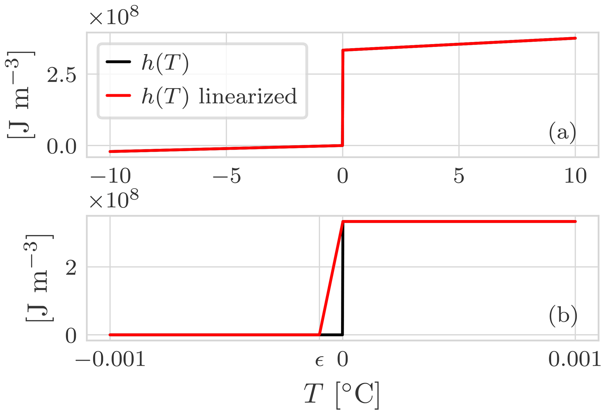
Figure E1(a) Comparison between the enthalpy function of pure water and the enthalpy function used in the numerical model. (b) Note that the energy jump due to the latent heat at Tm=0 ∘C has been linearized, and the steepness is controlled by the parameter ϵ.
The thermal conductivity is defined as
Defining the constant
the moving boundary function is
where the coefficient γ can be found by solving the following equation:
Finally the analytical solutions for problem with the Dirichlet boundary condition for the thawed and frozen zones are
Table E1Input parameters for the comparison between Neumann analytical solution and the numerical solution with the NCZ algorithm.

The solution for the Lunardini problem (i.e. the Lunardini solution) as described by McKenzie et al. (2007) is given by the following set of equations:
where T1, T2, and T3 are the temperatures at distance, x, from the temperature boundary for the frozen, partially frozen, and unfrozen zone respectively; erf and erfc are the error function and the complementary error function respectively; T0, Tm, Tf, and Ts are the temperatures of the initial condition, the solidus, the liquidus, and the boundary temperature, respectively; and α1 and α3 are the thermal diffusivities for the frozen and unfrozen zone respectively, defined as and , where C1 and C3 are the volumetric bulk-heat capacities of the frozen and unfrozen zones. The thermal diffusivity of the partially frozen zone is assumed to be constant across the transition region, and the thermal diffusivity with latent heat term included, α4, is defined as
where γd is the dry unit of soil solids, and , where ξ0 and ξf are the ratio of unfrozen water to soil solids for the fully thawed and frozen conditions respectively. For a time, t, in the region the temperature is T1 and X1(t) is given by
from the temperature is T2, where X(t) is given by
and for x≥X(t) the temperature is T3. The unknowns, ψ and γ, are solving the set of these two equations:
Table F1Input parameters for the comparison between the Lunardini analytical solution and the numerical solution with the NCZ algorithm.
a The first value refers to ∘C, the second value to ∘C, and the third value to ∘C.
As explained in Sect. 5, comparing the position of the zero isotherm after 100 years using three different time steps – hourly, daily, and 10 d – there is no significant deviation in the results. The larger deviation occurs when the zero isotherm is shallow: at the beginning of the thawing season as well as the freezing one.
At the beginning of the thawing season, Fig. G1, there is a time lag of about 1 month between the beginning of the thawing season for the hourly simulation and the 10 d simulation. This can be attributed to different surface temperature used to drive the simulations. In particular, in the case of the hourly simulation it is possible to see the oscillations of the position of the zero isotherm, panel (c), related to the oscillation of the surface temperature around 0 ∘C, panel (a).

Figure G1Detail of the beginning of the thawing season for the year 1999. Panel (a) shows the surface temperature for the hourly, the daily, and the 10 d simulations. Panel (b) shows the deviation of the position of the zero isotherm after 100 years between the hourly and the 10 d simulation, as well as between the daily and the 10 d simulation. Panel (c) shows the position of the zero isotherm after 100 years for the three simulations. In panel (b) there is a time lag of about 1 month between the beginning of thawing season for the hourly simulation and the 10 d one (dashed grey line). This can be attributed to the different surface temperature used to drive the simulations.
Figure G2 shows the detail of the freezing season. In panel (c) it is possible to note that when the zero isotherm is deep there is a good agreement between the three simulations. The main differences occur at the soil surface since with larger time steps the signal of the surface boundary condition is smoothed and does not oscillate around 0 ∘C. Moreover, by using an hourly time step and a daily time step it is possible to capture the joining of the downward and upward freezing front, while this is not possible with the 10 d time step since the joining occurs in between two consecutive time steps.
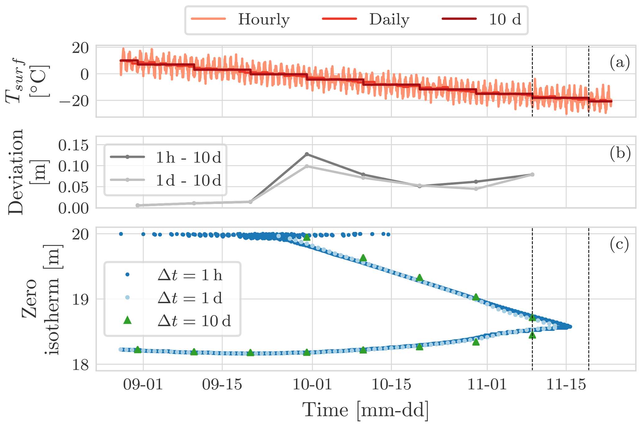
Figure G2Detail of the beginning of the freezing season for the year 1999. Panel (a) shows the surface temperature for the hourly, the daily, and the 10 d simulations. Panel (b) shows the deviation of the position of the zero isotherm after 100 years between the hourly and the 10 d simulation, as well as between the daily and the 10 d simulation. Panel (c) shows the position of the zero isotherm after 100 years for the three simulations. The joining of the downward and upward freezing front is captured by the hourly and the daily simulations (c). It is interesting to note that for the 10 d simulation the joining occurs in between two consecutive time steps.
As explained in Sect. 5, the maximum temperature profile, Fig. 12d, presents an “elbow” due to the so-called zero-curtain effect. The zero-curtain effect, Fig. G3, is the period of time during which the temperature remains nearly constant and very close to the freezing point because of the latent heat released during the phase change of water.
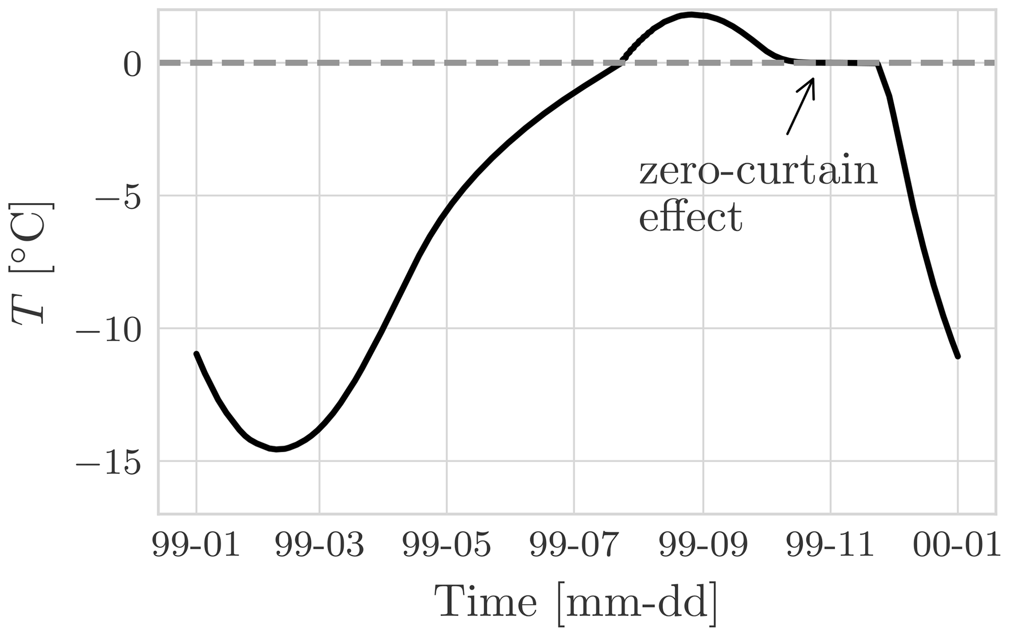
Figure G3Hourly temperature at 1.5 m depth for the year 1999. Note the prolonged period of 43 d (11 October until 23 November) when temperature remained within ±0.1 ∘C. This is the so-called zero-curtain effect, and it is due to latent heat of fusion that is continually released during the freezing of soil moisture.
Figure G4 shows the temperature envelopes for the hourly, the daily, and the 10 d simulations setting the thermal conductivity of water equal to the thermal conductivity of ice, λw=λi. It is interesting to note that mean temperature, panel (c), is constant throughout the soil column. The mean temperature is very close to the initial temperature profile that is also equal to the mean surface boundary condition.
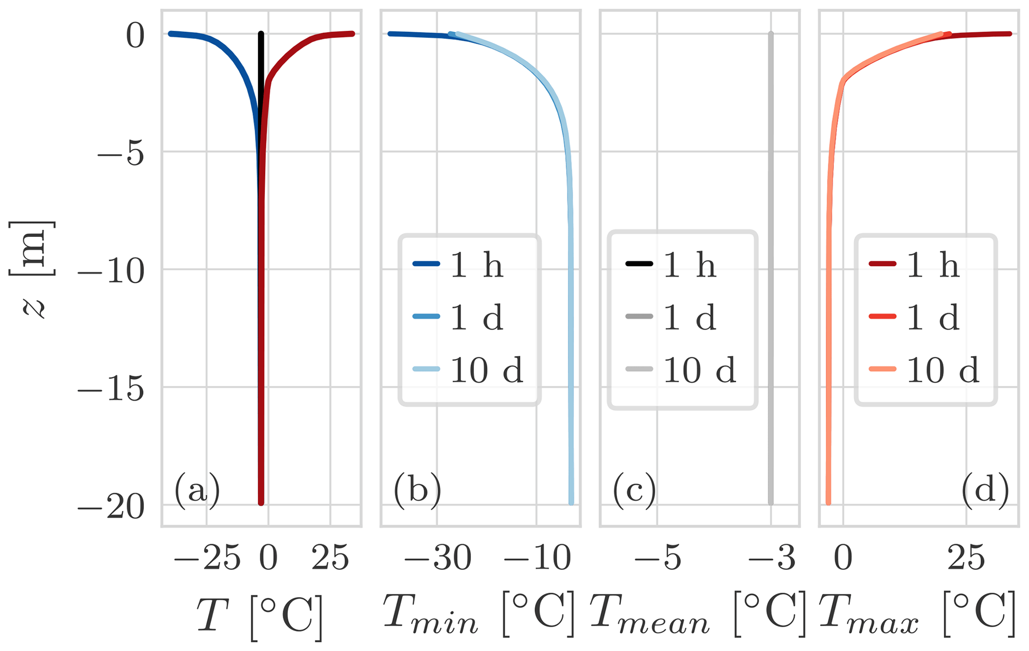
Figure G4Temperature profile envelope considering λw=λi. (a) The minimum, mean, and maximum temperature profile for the hourly simulation. Panels (b), (c), and (d) show the comparison of the minimum, mean, and maximum temperature profile respectively for the three simulations: with an hourly surface temperature boundary condition and Δt=1 h, with a daily surface temperature boundary condition and Δt=1 d, and with a 10 d surface temperature boundary condition and Δt=10 d. All three simulations last 100 years. Because λw=λi, the mean temperature, panel (c), is constant throughout the soil column, and it is not possible to appreciate the thermal offset. The mean temperature is very close to the initial temperature profile; the maximum error is 0.003 ∘C.
Figure G5 shows a comparison of the zero-isotherm position by using a coarser space discretization. Again, the three simulations with the hourly time step, the daily time step, and the 10 d time step are still in good agreement. By using a coarser spatial discretization, the zero isotherm, panel (c), presents some steps that are not present when using a finer grid (Fig. 11). Moreover, the joining of the downward and upward freezing front is not captured by the hourly or by the daily simulations.
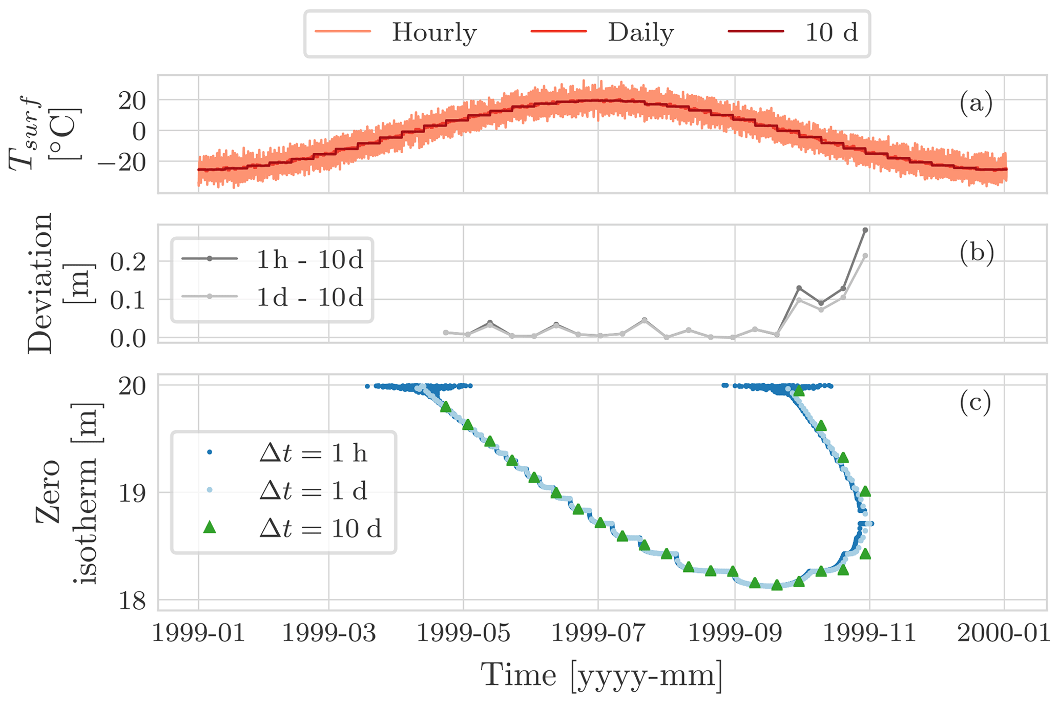
Figure G5Comparison of the position of the zero isotherm, panel (c), after 100 years of three simulations: using an hourly boundary condition with time step of Δt=1 h, using a daily boundary condition with a time step of Δt=1 d, and using a 10 d boundary condition with a time step of Δt=10 d. Panel (a) shows the surface temperature for the hourly, the daily, and the 10 d simulations. Panel (b) shows the deviation of the position of the zero isotherm after 100 years between the hourly and the 10 d simulation, as well as between the daily and the 10 d simulation. Panel (c) shows the position of the zero isotherm. It is interesting to note that all the three curves are characterized by the presence of some steps due to the usage of a coarser grid. This trend is independent of the size of the time step. Another consequence of this is that the joining of the downward and upward freezing front is not captured by the hourly or by the daily simulations.
Table G1Input parameters for the numerical tests.
a We used two different space discretizations. The thickness of the ground layer is parametrized as (Gubler et al., 2013).
For this numerical test we checked the mean number of iterations required to solve the non-linear system with the NCZ algorithm, the Newton–Raphson algorithm, and the globally convergent Newton algorithm. We performed a simulation lasting 1 year with a time step Δt=1 h and for different spatial discretizations. As can be seen in Table G2, neither the Newton–Raphson nor the globally convergent Newton converges: they always reach the maximum number of iterations allowed with a consequent increase in the computational cost.
Table G2Summary of the mean number of iterations for the NCZ algorithm, the Newton–Raphson algorithm (N. R.), and the globally convergent Newton algorithm (g. c. N.). The simulation lasts 1 year with a time step Δt=1 h. We considered different spatial discretizations. The tolerance has been rescaled with the water latent heat of fusion and the water density. The maximum number of iteration for each time step is 40. As can be seen the Newton–Raphson and the globally convergent Newton does not converge so it always reaches the maximum number of iterations allowed.
The source code is written in Java using the object-oriented programming paradigm. It can be found at https://github.com/geoframecomponents/FreeThaw1D (last access: 16 October 2020) (Tubini, 2020b). The OMS3 project can be found at https://github.com/GEOframeOMSProjects/OMS_FreeThaw1D (last access: 16 October 2020) (Tubini, 2020a). FreeThaw1D is deployed as an open-source code to work alone or inside the Object Modelling System version 3 framework (David et al., 2013). In the latter case it can be connected at run time with the many other components developed along with the GEOframe system (Formetta et al., 2014; Bancheri, 2017) for providing hydrometeorological forcings and other fluxes, like the evapotranspiration. The simulations presented here can be found at https://doi.org/10.5281/zenodo.4017668 (Tubini et al., 2020). The code must be run inside the OMS3 Console or using the dockerized version of OMS3. For setting up the environment, please follow the steps described in the README file present in the GitHub repository https://github.com/GEOframeOMSProjects/OMS_FreeThaw1D and in the GEOframe pages at https://geoframe.blogspot.com/2020/12/installations-of-2021-geoframe.html (last access: 28 January 2021). Once you have installed OMS3, please follow the instructions contained in Jupyter_Notebook\_README.ipynb and Jupyter_Notebook\00_FreeThaw1D.ipynb. They contain all the details about the simulation inputs and parameters.
Data presented in this paper can be found at https://doi.org/10.5281/zenodo.4017668 (Tubini et al., 2020).
NT, SG, and RR conceptualized the study; NT and RR developed the software; NT wrote the original draft; NT, SG, and RR reviewed and edited the manuscript. All the authors have read and agreed to the published version of the manuscript.
The authors declare that they have no conflict of interest.
The first author would like to thank Vincenzo Casulli and Michael Dumbser of the Department of Civil, Environmental and Mechanical Engineering at the University of Trento for their fruitful discussions on the numerical aspects of the work. We thank Andy Aschwanden, Ed Bueler, and Constantine Khrulev for their feedback regarding ice-sheet models and Samuel Morin for feedback regarding the model Crocus. We especially thank Matthieu Lafaysse and the anonymous reviewer for their constructive comments that helped to improve our paper.
This research has been supported by a PhD grant by the Department of Civil, Environmental and Mechanical Engineering at the University of Trento (Department of Excellence of MIUR) and by the Italian MIUR Project (PRIN 2017) “WATer mixing in the critical ZONe: observations and predictions under environmental changes” (WATZON; project code: 2017SL7ABC). In Canada, support was available through the NSERC Strategic Project “Improved Characterization of Permafrost Vulnerability to Support Decision Makers, Infrastructure, and Community Stewardship in the Northwest Territories” and NSERC PermafrostNet.
This paper was edited by Marie Dumont and reviewed by Matthieu Lafaysse and one anonymous referee.
Anderson, D. M. and Tice, A. R.: Predicting unfrozen water contents in frozen soils from surface area measurements, Highway research record, 393, 12–18, 1972. a
Andreas, E. L.: Handbook of physical constants and functions for use in atmospheric boundary layer studies, Cold Regions Research and Engineering Laboratory, US Army Engineer Research and Development Center, 2005. a
Aschwanden, A. and Blatter, H.: Meltwater production due to strain heating in Storglaciären, Sweden, J. Geophys. Res.-Earth Surf., 110, F04024, https://doi.org/10.1029/2005JF000328, 2005. a
Aschwanden, A. and Blatter, H.: Mathematical modeling and numerical simulation of polythermal glaciers, J. Geophys. Res., 114, F01027, https://doi.org/10.1029/2008JF001028, 2009. a, b, c, d, e, f
Aschwanden, A., Bueler, E., Khroulev, C., and Blatter, H.: An enthalpy formulation for glaciers and ice sheets, J. Glaciol., 58, 441–457, 2012. a, b
Bancheri, M.: A flexible approach to the estimation of water budgets and its connection to the travel time theory, PhD thesis, University of Trento, Trento, 2017. a
Bao, H., Koike, T., Yang, K., Wang, L., Shrestha, M., and Lawford, P.: Development of an enthalpy-based frozen soil model and its validation in a cold region in China, J. Geophys. Res.-Atmos., 121, 5259–5280, 2016. a, b, c
Bartelt, P. and Lehning, M.: A physical SNOWPACK model for the Swiss avalanche warning: Part I: numerical model, Cold Reg. Sci. Technol., 35, 123–145, 2002. a
Boone, A. and Etchevers, P.: An intercomparison of three snow schemes of varying complexity coupled to the same land surface model: Local-scale evaluation at an Alpine site, J. Hydrometeorol., 2, 374–394, 2001. a, b, c
Bouyoucos, G.: Degree of temperature to which soils can be cooled without freezing, Mon. Weather Rev., 48, 718–718, 1920. a
Bouyoucos, G. and McCool, M.: The freezing point method as a new means of measuring the concentration of the soil solution directly in the soil, Mich, Agr. Exp. Sta. Tech. Bull., 24, 44 pp., 1915. a
Bouyoucos, G. J.: An investigation of soil temperature and some of the most important facters influencing it, Technical Bulletin of Michigan Agriculture Experimental Station, 17, 1–196, 1913. a
Bouyoucos, G. J.: Movement of soil moisture from small capillaries to the large capillaries of the soil upon freezing, J. Agric. Res., 24, 427–432, 1923. a
Brugnano, L. and Casulli, V.: Iterative solution of piecewise linear systems, SIAM J. Sci. Comput., 30, 463–472, 2008. a
Brugnano, L. and Casulli, V.: Iterative solution of piecewise linear systems and applications to flows in porous media, SIAM J. Sci. Comput., 31, 1858–1873, 2009. a
Brun, E., Martin, E., Simon, V., Gendre, C., and Coleou, C.: An energy and mass model of snow cover suitable for operational avalanche forecasting, J. Glaciol., 35, 333–342, 1989. a
Brun, E., David, P., Sudul, M., and Brunot, G.: A numerical model to simulate snow-cover stratigraphy for operational avalanche forecasting, J. Glaciol., 38, 13–22, 1992. a, b, c
Callen, H. B.: Thermodynamics and an Introduction to Thermostatistics, John Wiley and Sons, Inc., Republic of Singapore, 1985. a
Casulli, V. and Walters, R. A.: An unstructured grid, three-dimensional model based on the shallow water equations, Int. J. Numer. Meth. Fluids, 32, 331–348, 2000. a
Casulli, V. and Zanolli, P.: A nested Newton-type algorithm for finite volume methods solving Richards' equation in mixed form, SIAM J. Sci. Comput., 32, 2255–2273, 2010. a, b, c, d, e, f, g, h, i, j, k, l
Casulli, V. and Zanolli, P.: Iterative solutions of mildly nonlinear systems, J. Comput. Appl. Math., 236, 3937–3947, 2012. a, b, c, d, e, f, g, h, i
Celia, M. A., Bouloutas, E. T., and Zarba, R. L.: A general mass-conservative numerical solution for the unsaturated flow equation, Water Resour. Res., 26, 1483–1496, 1990. a
Chistyakov, V.: On mappings of bounded variation, J. Dyn. Control Syst., 3, 261–289, 1997. a
Clow, G. D.: CVPM 1.1: a flexible heat-transfer modeling system for permafrost, Geosci. Model Dev., 11, 4889–4908, https://doi.org/10.5194/gmd-11-4889-2018, 2018. a, b
Dai, Y., Zeng, X., Dickinson, R. E., Baker, I., Bonan, G. B., Bosilovich, M. G., Denning, A. S., Dirmeyer, P. A., Houser, P. R., Niu, G., Dai, Y., Zeng, X., Dickinson, R. E., Baker, I., Bonan, G. B., Bosilovich, M. G., Denning, A. S., Dirmeyer, P. A., Houser, P. R., Niu, G., Oleson, K. W., Schlosser, C. A., and Yang, Z.-L.: The common land model, B. Am. Meteorol. Soc., 84, 1013–1024, 2003. a
Dall'Amico, M.: Coupled water and heat transfer in permafrost modeling, PhD thesis, University of Trento, Trento, 2010. a, b, c, d
Dall'Amico, M., Endrizzi, S., Gruber, S., and Rigon, R.: A robust and energy-conserving model of freezing variably-saturated soil, The Cryosphere, 5, 469–484, https://doi.org/10.5194/tc-5-469-2011, 2011. a, b, c, d, e, f, g, h, i, j
D'Amboise, C. J. L., Müller, K., Oxarango, L., Morin, S., and Schuler, T. V.: Implementation of a physically based water percolation routine in the Crocus/SURFEX (V7.3) snowpack model, Geosci. Model Dev., 10, 3547–3566, https://doi.org/10.5194/gmd-10-3547-2017, 2017. a
David, O., Ascough II, J. C., Lloyd, W., Green, T. R., Rojas, K., Leavesley, G. H., and Ahuja, L. R.: A software engineering perspective on environmental modeling framework design: The Object Modeling System, Environ. Model. Softw., 39, 201–213, 2013. a
De Lorenzo, S., Di Renzo, V., Civetta, L., D'antonio, M., and Gasparini, P.: Thermal model of the Vesuvius magma chamber, Geophys. Res. Lett., 33, L17302, https://doi.org/10.1029/2006GL026587, 2006. a
Ekici, A., Beer, C., Hagemann, S., Boike, J., Langer, M., and Hauck, C.: Simulating high-latitude permafrost regions by the JSBACH terrestrial ecosystem model, Geosci. Model Dev., 7, 631–647, https://doi.org/10.5194/gmd-7-631-2014, 2014. a, b
Endrizzi, S., Gruber, S., Dall'Amico, M., and Rigon, R.: GEOtop 2.0: simulating the combined energy and water balance at and below the land surface accounting for soil freezing, snow cover and terrain effects, Geosci. Model Dev., 7, 2831–2857, https://doi.org/10.5194/gmd-7-2831-2014, 2014. a
Foley, J. A., Prentice, I. C., Ramankutty, N., Levis, S., Pollard, D., Sitch, S., and Haxeltine, A.: An integrated biosphere model of land surface processes, terrestrial carbon balance, and vegetation dynamics, Global Biogeochem. Cycles, 10, 603–628, 1996. a
Formetta, G., Antonello, A., Franceschi, S., David, O., and Rigon, R.: Hydrological modelling with components: A GIS-based open-source framework, Environ. Model. Softw., 55, 190–200, 2014. a
Goodrich, L.: Some results of a numerical study of ground thermal regimes, in: Proceedings of the Third International Conference on Permafrost, National Research Council of Canada, Ottawa, Edmonton, Canada, 1978. a
Goodrich, L.: The influence of snow cover on the ground thermal regime, Can. Geotech. J., 19, 421–432, 1982. a, b, c
Greve, R.: Application of a polythermal three-dimensional ice sheet model to the Greenland ice sheet: response to steady-state and transient climate scenarios, J. Climate, 10, 901–918, 1997a. a, b
Greve, R.: A continuum–mechanical formulation for shallow polythermal ice sheets, Philos. T. R. Soc. Lond. A, 355, 921–974, 1997b. a, b, c
Greve, R. and Blatter, H.: Comparison of thermodynamics solvers in the polythermal ice sheet model SICOPOLIS, Polar Sci., 10, 11–23, 2016. a, b
Gubler, S., Endrizzi, S., Gruber, S., and Purves, R. S.: Sensitivities and uncertainties of modeled ground temperatures in mountain environments, Geosci. Model Dev., 6, 1319–1336, https://doi.org/10.5194/gmd-6-1319-2013, 2013. a, b
Hansson, K., Šimünek, J., Mizoguchi, M., Lundin, L.-C., and Van Genuchten, M. T.: Water flow and heat transport in frozen soil, Vadose Zone J., 3, 693–704, 2004. a, b, c
Harris, C., Arenson, L. U., Christiansen, H. H., Etzelmüller, B., Frauenfelder, R., Gruber, S., Haeberli, W., Hauck, C., Hölzle, M., Humlum, O., Isaksen, K., Kääb, A., Kern-Lütschg, M. A., Lehning, M., Matsuoka, N., Murton, J. B., Noetzli, J., Phillips, M., Ross, N., Seppälä, M., Springman, S. M., and Vonder Mühll, D.: Permafrost and climate in Europe: Monitoring and modelling thermal, geomorphological and geotechnical responses, Earth-Science Rev., 92, 117–171, 2009. a
Hewitt, I. and Schoof, C.: A model for polythermal ice incorporating gravity-driven moisture transport, J. Fluid Mech., 797, 504–535, 2016. a, b
Hollesen, J., Elberling, B., and Jansson, P.-E.: Future active layer dynamics and carbon dioxide production from thawing permafrost layers in Northeast Greenland, Global Change Biol., 17, 911–926, 2011. a
Hu, H. and Argyropoulos, S. A.: Mathematical modelling of solidification and melting: a review, Model. Simul. Mater. Sc., 4, 371–396, 1996. a
InterFrost Project: InterFrost Project, available at: https://wiki.lsce.ipsl.fr/interfrost/doku.php?id=test_cases:one, last access: 20 August 2020. a
Jansson, P. and Karlberg, L.: Coupled heat and mass transfer model for soil-plant-atmosphere systems, Royal Institute of Technology, Dept. of Civil and Environmental Engineering, Stockholm, 2011. a
Kozlowski, T.: A semi-empirical model for phase composition of water in clay–water systems, Cold Reg. Sci. Technol., 49, 226–236, 2007. a
Krinner, G., Viovy, N., de Noblet-Ducoudré, N., Ogée, J., Polcher, J., Friedlingstein, P., Ciais, P., Sitch, S., and Prentice, I. C.: A dynamic global vegetation model for studies of the coupled atmosphere-biosphere system, Global Biogeochem. Cycles, 19, GB1015, https://doi.org/10.1029/2003GB002199, 2005. a
Kurylyk, B. L. and Watanabe, K.: The mathematical representation of freezing and thawing processes in variably-saturated, non-deformable soils, Adv. Water Resour., 60, 160–177, 2013. a, b
Kurylyk, B. L., MacQuarrie, K. T., and McKenzie, J. M.: Climate change impacts on groundwater and soil temperatures in cold and temperate regions: Implications, mathematical theory, and emerging simulation tools, Earth-Sci. Rev., 138, 313–334, 2014a. a
Kurylyk, B. L., McKenzie, J. M., MacQuarrie, K. T., and Voss, C. I.: Analytical solutions for benchmarking cold regions subsurface water flow and energy transport models: One-dimensional soil thaw with conduction and advection, Adv. Water Resour., 70, 172–184, 2014b. a, b, c
Lafaysse, M., Cluzet, B., Dumont, M., Lejeune, Y., Vionnet, V., and Morin, S.: A multiphysical ensemble system of numerical snow modelling, The Cryosphere, 11, 1173–1198, https://doi.org/10.5194/tc-11-1173-2017, 2017. a
Langham, E.: Phase equilibria of veins in polycrystalline ice, Canadian J. Earth Sci., 11, 1280–1287, 1974. a, b
Lawrence, D., Fisher, R., Koven, C., Oleson, K., Swenson, S., and Vertenstein, M.: CLM5 documentation, Tech. rep., Tech. rep., National Center for Atmospheric Research, Boulder, CO, 2019. a
Lehning, M., Bartelt, P., Brown, B., Russi, T., Stöckli, U., and Zimmerli, M.: SNOWPACK model calculations for avalanche warning based upon a new network of weather and snow stations, Cold Reg. Sci. Technol., 30, 145–157, 1999. a, b, c
Lewis, R. and Ravindran, K.: Finite element simulation of metal casting, Int. J. Numer. Meth. Eng., 47, 29–59, 2000. a
Lliboutry, L. and Duval, P.: Various isotropic and anisotropic ices found in glaciers and polar ice caps and their corresponding rheologies, Ann. Geophys., 3, 207–224, 1985. a
Lunardini, V. J.: Freezing of soil with an unfrozen water content and variable thermal properties, Tech. Rep. 88-2, US Army Corps of Engineers, Cold Regions Research & Engineering Laboratory, Hanover, NH, 1988. a, b
Marchenko, S., Romanovsky, V., and Tipenko, G.: Numerical modeling of spatial permafrost dynamics in Alaska, in: Proceedings of the ninth international conference on permafrost, 29, 1125–1130, Institute of Northern Engineering, University of Alaska, Fairbanks, 2008. a
McKenzie, J. M. and Voss, C. I.: Permafrost thaw in a nested groundwater-flow system, Hydrogeol. J., 21, 299–316, 2013. a
McKenzie, J. M., Voss, C. I., and Siegel, D. I.: Groundwater flow with energy transport and water–ice phase change: numerical simulations, benchmarks, and application to freezing in peat bogs, Adv. Water Resour., 30, 966–983, 2007. a, b, c, d, e, f
Mongibello, L., Bianco, N., Caliano, M., and Graditi, G.: Numerical simulation of an aluminum container including a phase change material for cooling energy storage, Applied System Innovation, 1, 34, 2018. a
Morin, S., Lejeune, Y., Lesaffre, B., Panel, J.-M., Poncet, D., David, P., and Sudul, M.: An 18-yr long (1993–2011) snow and meteorological dataset from a mid-altitude mountain site (Col de Porte, France, 1325 m alt.) for driving and evaluating snowpack models, Earth Syst. Sci. Data, 4, 13–21, https://doi.org/10.5194/essd-4-13-2012, 2012. a
Nazzi Ehms, J. H., De Césaro Oliveski, R., Oliveira Rocha, L. A., Biserni, C., and Garai, M.: Fixed grid numerical models for solidification and melting of phase change materials (PCMs), Appl. Sci., 9, 4334, 2019. a
Nedjar, B.: An enthalpy-based finite element method for nonlinear heat problems involving phase change, Comput. Struct., 80, 9–21, 2002. a
Nicolsky, D., Romanovsky, V., Alexeev, V., and Lawrence, D.: Improved modeling of permafrost dynamics in a GCM land-surface scheme, Geophys. Res. Lett., 34, L08501, https://doi.org/10.1029/2007GL029525, 2007a. a, b
Nicolsky, D. J., Romanovsky, V. E., and Tipenko, G. S.: Using in-situ temperature measurements to estimate saturated soil thermal properties by solving a sequence of optimization problems, The Cryosphere, 1, 41–58, https://doi.org/10.5194/tc-1-41-2007, 2007.b. a, b, c
Nye, J. F. and Frank, F. C.: Hydrology of the intergranular veins in a temperate glacier.InInternational Association of Scientific Hydrology Publication, Symp. Cambridge, 1969, Hydrol. Glaciers, 95, 157–161, 1973. a
Oleson, K. W., Dai, Y., Bonan, G., Bosilovich, M., Dickinson, R., Dirmeyer, P., Hoffman, F., Houser, P., Levis, S., Niu, G.-Y., Thornton, P., Vertenstein, M., Yang, Z.-L., and Zeng, X.: Technical description of the Community Land Model (CLM), Tech. rep., NCAR, Boulder, Colorado, 2004. a, b
Painter, S. L.: Three-phase numerical model of water migration in partially frozen geological media: model formulation, validation, and applications, Comput. Geosci., 15, 69–85, 2011. a, b
Paniconi, C. and Putti, M.: A comparison of Picard and Newton iteration in the numerical solution of multidimensional variably saturated flow problems, Water Resour. Res., 30, 3357–3374, 1994. a, b
Rempel, A. W., Wettlaufer, J., and Worster, M. G.: Premelting dynamics in a continuum model of frost heave, J. Fluid Mech., 498, 227–244, 2004. a, b
Rigon, R., Bertoldi, G., and Over, T. M.: GEOtop: A distributed hydrological model with coupled water and energy budgets, J. Hydrometeorol., 7, 371–388, 2006. a
Riseborough, D., Shiklomanov, N., Etzelmüller, B., Gruber, S., and Marchenko, S.: Recent advances in permafrost modelling, Permafrost Periglac. Process., 19, 137–156, 2008. a, b, c
Roe, P. L.: Approximate Riemann solvers, parameter vectors, and difference schemes, J. Comput. Phys., 43, 357–372, 1981. a, b
Ruhaak, W., Anbergen, H., Grenier, C., McKenzie, J., Kurylyk, B., Molson, J., Roux, N., and Sass, I.: Benchmarking numerical freeze/thaw models, Energy Procedia, 76, 301–310, 2015. a
Schuur, E. A. G., David McGuire, A., Schädel, C., Grosse, G., Harden, J. W., Hayes, D. J., Hugelius, G., Koven, C. D., Kuhry, P., Lawrence, D. M., Natali, S. M., Olefeldt, D., Romanovsky, V. E., Schaefer, K., Turetsky, M. R., Treat, C. C., and Vonk, J. E.: Climate change and the permafrost carbon feedback, Nature, 520, 171–179, 2015. a
Sergueev, D., Tipenko, G., Romanovsky, V., and Romanovskii, N.: Mountain permafrost thickness evolution under influence oflong-term climate fluctuations (results of numerical simulation), in: Proceedings of the VII International Permafrost Conference, Switzerland, 21–25 July, 1017–1021, 2003. a, b
Sheshukov, A. Y. and Nieber, J. L.: One-dimensional freezing of nonheaving unsaturated soils: Model formulation and similarity solution, Water Resour. Res., 47, W11519, https://doi.org/10.1029/2011WR010512, 2011. a
Shewchuk, J. R.: An Introduction to the Conjugate Gradient Method Without the Agonizing Pain, Tech. rep., USA, 1994. a
Streletskiy, D. A., Suter, L. J., Shiklomanov, N. I., Porfiriev, B. N., and Eliseev, D. O.: Assessment of climate change impacts on buildings, structures and infrastructure in the Russian regions on permafrost, Environ. Res. Lett., 14, 025003, https://doi.org/10.1088/1748-9326/aaf5e6, 2019. a
Tan, X., Chen, W., Tian, H., and Cao, J.: Water flow and heat transport including ice/water phase change in porous media: numerical simulation and application, Cold Reg. Sci. Technol., 68, 74–84, 2011. a
Teng, J., Kou, J., Yan, X., Zhang, S., and Sheng, D.: Parameterization of soil freezing characteristic curve for unsaturated soils, Cold Reg. Sci. Technol., 170, 102928, https://doi.org/10.1016/j.neubiorev.2019.07.019, 2020. a
Tubini, N.: OMS project, https://github.com/GEOframeOMSProjects/OMS_FreeThaw1D [Code], last access: 16 October 2020a. a
Tubini, N.: source code, https://github.com/geoframecomponents/FreeThaw1D [Code], last access: 16 October 2020b. a
Tubini, N., Gruber, S., and Rigon, R.: FreeThaw1D (Version v-0.98) [Code], Zenodo, https://doi.org/10.5281/zenodo.4017668, 2020. a
Verseghy, D. L.: CLASS – A Canadian land surface scheme for GCMs. I. Soil model, Int. J. Climatol., 11, 111–133, 1991. a
Vionnet, V., Brun, E., Morin, S., Boone, A., Faroux, S., Le Moigne, P., Martin, E., and Willemet, J.-M.: The detailed snowpack scheme Crocus and its implementation in SURFEX v7.2, Geosci. Model Dev., 5, 773–791, https://doi.org/10.5194/gmd-5-773-2012, 2012. a
Voller, V. and Cross, M.: Accurate solutions of moving boundary problems using the enthalpy method, Int. J. Heat Mass Transf., 24, 545–556, 1981. a
Voller, V. R.: Fast implicit finite-difference method for the analysis of phase change problems, Numer. Heat Transf., 17, 155–169, 1990. a
Voller, V. R., Swaminathan, C., and Thomas, B. G.: Fixed grid techniques for phase change problems: a review, Int. J. Numer. Meth., 30, 875–898, 1990. a, b, c, d, e, f, g
Voss, C. I. and Provost, A.: SUTRA: A model for 2D or 3D saturated-unsaturated, variable-density ground-water flow with solute or energy transport, Tech. rep., U.S. Geological Survey Water-Resources Investigations Report, Reston, Virginia, 2002. a
Vuik, C.: Some historical notes about the Stefan problem, Nieuw Arch. Wiskd., 11, 157–167, 1993. a
Walvoord, M. A. and Kurylyk, B. L.: Hydrologic impacts of thawing permafrost – A review, Vadose Zone J., 15, 1–20, 2016. a, b
Wang, T., Ottlé, C., Boone, A., Ciais, P., Brun, E., Morin, S., Krinner, G., Piao, S., and Peng, S.: Evaluation of an improved intermediate complexity snow scheme in the ORCHIDEE land surface model, J. Geophys. Res.-Atmos., 118, 6064–6079, 2013. a, b
Watanabe, K. and Mizoguchi, M.: Amount of unfrozen water in frozen porous media saturated with solution, Cold Reg. Sci. Technol., 34, 103–110, 2002. a, b
Watanabe, K., Kito, T., Wake, T., and Sakai, M.: Freezing experiments on unsaturated sand, loam and silt loam, Ann. Glaciol., 52, 37–43, 2011. a
Westermann, S., Schuler, T. V., Gisnås, K., and Etzelmüller, B.: Transient thermal modeling of permafrost conditions in Southern Norway, The Cryosphere, 7, 719–739, https://doi.org/10.5194/tc-7-719-2013, 2013. a, b
Westermann, S., Langer, M., Boike, J., Heikenfeld, M., Peter, M., Etzelmüller, B., and Krinner, G.: Simulating the thermal regime and thaw processes of ice-rich permafrost ground with the land-surface model CryoGrid 3, Geosci. Model Dev., 9, 523–546, https://doi.org/10.5194/gmd-9-523-2016, 2016. a
Wever, N., Fierz, C., Mitterer, C., Hirashima, H., and Lehning, M.: Solving Richards Equation for snow improves snowpack meltwater runoff estimations in detailed multi-layer snowpack model, The Cryosphere, 8, 257–274, https://doi.org/10.5194/tc-8-257-2014, 2014. a
Zhang, Y., Chen, W., and Cihlar, J.: A process-based model for quantifying the impact of climate change on permafrost thermal regimes, J. Geophys. Res.-Atmos., 108, 4695, 2003. a
Zhang, Y., Carey, S. K., and Quinton, W. L.: Evaluation of the algorithms and parameterizations for ground thawing and freezing simulation in permafrost regions, J. Geophys. Res.-Atmos., 113, D17116, https://doi.org/10.1029/2007JD009343, 2008. a, b, c
- Abstract
- Introduction
- The governing equation and their numerical issues
- A soil heat-transfer model using the NCZ algorithm
- Analytical benchmarks
- Numerical test
- Conclusions
- Appendix A: Commonly used simulation software
- Appendix B: Pseudocode
- Appendix C: Fully implicit formulation and the problem of the thermal conductivity
- Appendix D: Enthalpy and internal energy
- Appendix E: Neumann analytical derivation
- Appendix F: Lunardini analytical derivation
- Appendix G: Numerical test
- Code availability
- Data availability
- Author contributions
- Competing interests
- Acknowledgements
- Financial support
- Review statement
- References