Geographic variation and temporal trends in ice phenology in Norwegian lakes during the period 1890–2020

Long-term observations of ice phenology in lakes are ideal for studying climatic variation in time and space. We used a large set of observations from 1890 to 2020 of the timing of freeze-up and break-up, and the length of ice-free season, for 101 Norwegian lakes to elucidate variation in ice phenology across time and space. The dataset of Norwegian lakes is unusual, covering considerable variation in elevation (4–1401 m a.s.l.) and climate (from oceanic to continental) within a substantial latitudinal and longitudinal gradient (58.2–69.9^∘ N, 4.9–30.2^∘ E).

The average date of ice break-up occurred later in spring with increasing elevation, latitude and longitude. The average date of freeze-up and the length of the ice-free period decreased significantly with elevation and longitude. No correlation with distance from the ocean was detected, although the geographical gradients were related to regional climate due to adiabatic processes (elevation), radiation (latitude) and the degree of continentality (longitude). There was a significant lake surface area effect as small lakes froze up earlier due to less volume. There was also a significant trend that lakes were completely frozen over later in the autumn in recent years. After accounting for the effect of long-term trends in the large-scale North Atlantic Oscillation (NAO) index, a significant but weak trend over time for earlier ice break-up was detected.

An analysis of different time periods revealed significant and accelerating trends for earlier break-up, later freeze-up and completely frozen lakes after 1991. Moreover, the trend for a longer ice-free period also accelerated during this period, although not significantly.

An understanding of the relationship between ice phenology and geographical parameters is a prerequisite for predicting the potential future consequences of climate change on ice phenology. Changes in ice phenology will have consequences for the behaviour and life cycle dynamics of the aquatic biota.

1 Introduction

The surface area of lakes makes up a substantial part (15 %–40 %) of the arctic and sub-arctic regions of the Northern Hemisphere (Brown and Duguay, 2010). Most of these lakes freeze over annually. In addition to its substantial biological importance (Prowse, 2001), this annual freezing has significant repercussions for transportation, local cultural identity and religion (Magnusson et al., 2000; Prowse et al., 2011; Sharma et al., 2016; Knoll et al., 2019). The importance of freshwater and ice formation for people has resulted in the monitoring of freezing and thawing of lake ice for centuries (Sharma et al., 2016).

Lakes and their ice phenology are effective sentinels of climate change (Adrian et al., 2009) and ice phenology has been studied extensively (e.g. reviewed by Brown and Duguay, 2010). In general, freeze-up and break-up have changed over time, freeze-up occurs later and break-up appears earlier despite different timespans on global (Magnuson et al., 2000 (1846–1995); Benson et al., 2012 (1855–2005); Sharma and Magnusson, 2014 (1854–2004); Du et al., 2017 (2002–2015)), regional (Duguay et al., 2006 (1952–2000); Mishra et al., 2011 (1916–2007); Hewitt et al., 2018 (1981–2015)) and local scales (Choiński et al., 2015 (1961–2010); Takács et al., 2018 (1774–2017)). Despite these general results, the strength of the trends varies among studies. The time of freeze-up was delayed by 0.3 to 5.7 d per decade (Benson et al., 2012; Magnusson et al., 2000), whereas the timing of ice break-up was delayed by between 0.2 and 6.3 d per decade (Mishra et al., 2011; Magnusson et al., 2000). Some of this variation is a consequence of differences in the length of the study period, covering from more than a century to just a single decade. However, based on time series for 2000–2013 from 13 300 arctic lakes, Šmejkalova et al. (2016) showed significant and more dramatic trends in earlier start and end of break-up in northern Europe as the rate was 0.10 and 0.14 d yr⁻¹, respectively, and that this change was significantly correlated with the 0 ^∘C isotherm. The wide variation in time period and the particular time period studied is important to consider when trying to compare the strength of trends in ice phenology parameters as significant associations with ice break-up and oscillations (2–67 years) have been documented (Sharma and Magnusson, 2014). Global mean temperature has changed considerably since 1880 (Hansen et al., 2006), and the change (increase) in temperature is particularly evident in later decades (IPCC, 2007; Benson et al., 2012). By dividing data from the 1976–2005 period into shorter timer periods, Newton and Mullan (2020) showed, for Fennoscandia, an increase in the magnitude of the general trend in earlier break-up in 1991–2005 compared to earlier periods. In North America the trend was for earlier break-up, but it was neither spatially nor temporally consistently explained by local or regional variation in climate (Jensen et al., 2007). In a recent study, Filazzola et al. (2020) showed that unusually shorter ice cover periods are becoming more frequent and even shorter, especially since 1990.

In Fennoscandia, recording ice phenology has long traditions due to the importance of frozen lakes and rivers for transport and recreation (Sharma et al., 2016). Data from Swedish and Finnish lakes have been studied in detail (e.g. Eklund, 1999; Kuusisto and Elo, 2000; Livingstone, 2000; Yoo and D'Odorico, 2002; Blenckner et al., 2004; Korhonen, 2006; Palecki and Barry, 1986). Based on Swedish data for the period 1710–2000, Eklund (1999) showed that ice break-up did not change from 1739 to 1909, became 5 d earlier in the period 1910–1988 and still 13 d earlier during the final period (1988–1999). Furthermore, ice freeze-up was later in the 1931–1999 period than in the 1901–1930 period. Similarly, stronger trends in both freeze-up and break-up in the last decade of the 1950–2009 time period have been shown for both Finnish and Karelian lakes (Blenckner et al., 2004; Efremova et al., 2004; Korhonen, 2006). Moreover, Blenckner et al. (2004) showed that large variability was apparent south of 62^∘ N, indicating that lakes in southern Sweden were more influenced by large-scale climate effects (such as the North Atlantic Oscillation; NAO; Hurrell, 1995) than northern lakes. This pattern was explained by the mountain range between Norway and Sweden affecting the regional circulation in the north. The large-scale anomaly in the NAO in the winter season shifts between strong westerly winds with warm and moist air and cold, easterly dry winds across the North Atlantic and western Europe. The positive phases of NAO are associated with milder and rainy delayed winters and early springs in northern Europe (Hurrell, 1995). This significantly affects the timing of ice break-up in lakes (Palecki and Barry, 1986; Livingstone, 2000; Yoo and D'Odorico, 2002). However, Yoo and D'Odorico (2002) argued that climatic forcing such as CO₂-induced regional and global warming may have a pronounced effect leading to earlier break-up. On the other hand, George et al. (2004) showed that ice correlations (freeze-up and length of the period of ice cover) differed strongly between Windermere, situated close to the Irish Sea in northwestern England, and Pääjärvi, situated some distance from the Baltic sea in southern Finland. The number of days with ice has fallen dramatically for lake Windermere, whereas no such trend was detected for Pääjärvi. They postulated that the position of the boundary between the oceanic and continental climate regimes can change and produce a significant shift in winter dynamics of lakes located near this zone. In addition to this effect between climate zones, the boundary of the 0 ^∘C isotherm is important as it strongly affects ice formation and break-up (Brown and Duguay, 2010; Filazzola et al., 2020).

Despite the fact that registration of ice phenology has been undertaken in a large number of lakes and rivers in Norway, as early as 1818 in some lakes (http://www.nve.no, last access: 10 October 2020), few lakes have been studied in detail and no country-wide analysis has been done. Trends in freeze-up and break-up have been analysed for two subalpine lakes in central Norway (Kvambekk and Melvold, 2010; Tvede, 2004; Solvang, 2013). Although not covering the exact same period, both freeze-up and break-up show different trends in the two lakes. Although geographically close to lakes in Sweden and Finland, Norwegian lakes demonstrate considerably more variation in topography and climate. Norway covers most of the Scandinavian north–south mountain ridge with several summits above 2300 m a.s.l., while the highest mountains in Sweden and Finland only reach 2106 and 1328 m a.s.l., respectively. This mountain ridge ensures that Sweden and Finland generally have a continental climate, contrary the complex climate in Norway with oceanic climate in the west and south, continental climate in the east along the Swedish and Finnish border, and tundra and subarctic climates in the mountain regions in the southern and northern parts. Norwegian lakes, situated in the western parts of the Scandinavian peninsula, encompass a large variation in elevation over short distances as well as substantial latitudinal and longitudinal variation. A large and complex coast also introduces considerable climate variability. This makes Norwegian lakes well suited for testing the effect of climate change on ice phenology, also in relation to elevation.

In the present study, we have analysed long-term (1890–2020) observations of lake freeze-up, ice break-up and length of ice-free period in 101 Norwegian lakes. The lakes cover a broad range of climatic zones described by geographical parameters (elevation, latitude and longitude), as well as lake characteristics (area, water inflow and water level amplitude). The main aim of the analyses was to detect potential temporal trends in ice phenology while adjusting for both geographical parameters and lake characteristics.

2 Material and methods

2.1 Lakes studied

We collated observations from 101 Norwegian lakes, covering a wide range in latitude (58.2–69.9^∘ N), longitude (4.9–30.2^∘ E) and elevation (4–1401 m a.s.l.). The lakes are situated in three major climatic zones (boreal, subalpine, alpine) and with varying distances from the ocean. Thus, they differ widely in several geographic characteristics (Fig. 1, Appendix A). Most of the lakes are relatively small (median area 6.9 km²), although the dataset also includes Norway's largest lake, Mjøsa (369.3 km²). Their catchment areas vary between 7.1 and 18 101.9 km² (median 235 km²), and mean annual inflow to the lakes varies between 5.6×10⁶ and 9935.7×10⁶ m³ yr⁻¹ (median 256×10⁶ m³ yr⁻¹). About 50 % of the lakes (N=53) were developed for hydropower production with an annual water level variation varying from 1 to 30.3 m. The lake and catchment information was extracted from Norwegian Water Resources and Energy Directorate website http://www.nve.no (last access: 10 October 2020).

Figure 1 Topographic map of Norway with the 101 lakes included in the analysis. Information on the locations and names of the lakes is given in Table A1.

2.2 Ice observations

Observations of the timing of ice formation on the lakes in autumn and ice break-up in spring were undertaken visually or by fixed-location video cameras. The data were made available by the Norwegian Water Resources and Energy Directorate (NVE), the hydropower association Glommens og Laagens Brukseierforening, or by private persons. NVE operates a national hydrological database that contains information on ice conditions. The first observations are from 1818, but substantial records started in the 1890s. Video cameras have now replaced visual observations in some lakes. Satellite data are also being increasingly used to detect ice cover or open water. In our dataset, we have included lakes with more than 7 years of observations for at least one ice phenology variable in the analysis. This resulted in 101 lakes of which 76 have a registration period exceeding 30 years (Fig. 2, Appendix B). The average length of the data series was 53 years (range 11–149 years).

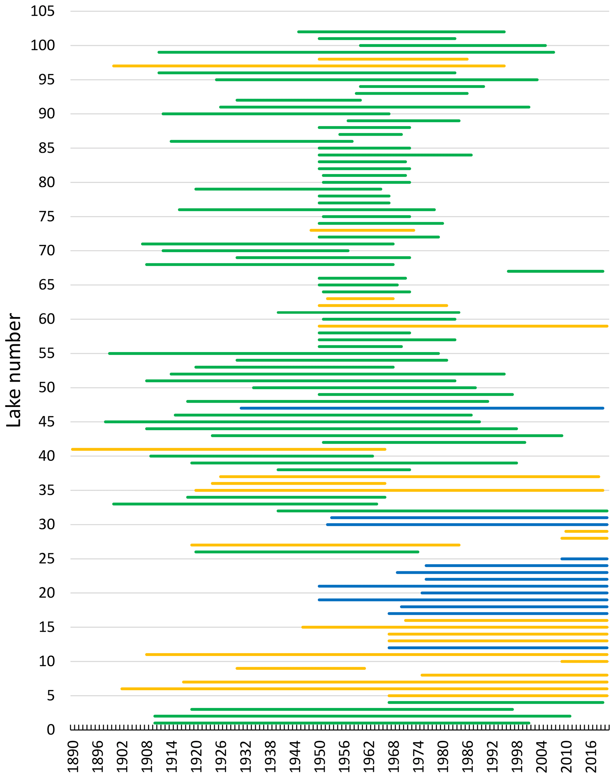
Figure 2 Chart showing the registration periods (1890–2020) for ice phenology (ice freeze-up, frozen lake and ice break-up) for individual lakes. For Lake 41, registration started in 1818 but was not continuous. In several data series there are years with missing registration of variables. The colour indicates elevation for each lake (green: < 500 m a.s.l.; yellow: 500–1000 m a.s.l.; blue: > 1000 m a.s.l.). For information on each lake see Appendix A and B.

Prior to 2000, most observations of ice phenology were carried out manually by NVE observers, power company employees, farmers and landowners. Afterwards web cameras and remote sensing became increasingly important. In most years, registrations were on a daily basis. After 2000, personnel conducted weekly observations, and in these cases remote sensing was used to improve accuracy. Registrations by personnel were conducted at the shore. Thus, the accuracy is high for the date of freeze-up, whereas the setting of the date of a completely ice-covered lake and break-up have an uncertainty of a couple of days.

The date of ice break-up was set when the lake was estimated to be free of ice based on the available observations. The length of the ice-free period during summer was then estimated as the difference between the day of freeze-up in the autumn and the day of ice break-up in spring. All dates are given as Julian day number during the year (1 January is day 1). For some lakes in certain years ice formation started in winter after 1 January. For these years the day number was extended past the normal 365 d. The observations were always made at the same site in each lake. The date of freeze-up was set when the first formation of ice was observed. Subsequent temporary ice-free periods, often due to mild weather combined with strong winds, did not change this date. The date when the whole lake was covered by ice was also noted, when possible. This date is more variable, and information is frequently missing. It would require extensive travel and several observation points to ascertain this date with high certainty, unless there are time-lapse cameras or satellite data. We have a total of 4371 observations on ice break-up, 3035 observations of freeze-up, 4221 observations of when the lakes were completely frozen over, and 2808 observations of the length of the ice-free period.

Some of the lakes are used as hydropower reservoirs, and thus within-year water level variation may differ from the normal annual cycle. For such lakes we have included information on the year of regulation and the maximum amplitude of water level variation. Although we do not have information on exact water level variation within a given year, maximum and minimum occurs when freeze-up and break-up normally take place, respectively.

For one particular large lake there are observations from two different locations (called Tustervatn and Røssvatn) that were partly overlapping in time. The observations of the time of ice break-up and ice freeze-up were strongly and positively correlated. The correlation between the two different estimates of time of freeze-up (r=0.501, n=37, p=0.002) was lower than for the time of break-up (r=0.887, n=38, p<0.001). There was no tendency for a particular temporal trend for this particular lake, so we have used the longest of the two time series in the analyses.

2.3 Climate data

As a potential large-scale climate driver, especially impacting ice break-up, we used the North Atlantic Oscillation (NAO) index. We therefore extracted the principal component analysis (PCA)-based winter (December to March) NAO index (National Center for Atmospheric Research Staff (Eds.), last modified 10 September 2019: https://climatedataguide.ucar.edu/climate-data/hurrell-north-atlantic-oscillation-nao-index-pc-based, last access: 28 October 2020). Variation in winter NAO is known to impact on winter temperature and precipitation, depending on location (Hurrell, 1995; Stenseth et al., 2003). An elevated index leads to mild and wet winters in Europe, while a low index leads to cold and dry winters. The PCA-based winter NAO index covers the period from 1898 to 2020. The winter index covers the period December–February, and we used this index to test for large-scale variation in timing of ice break-up as the winter index influences both winter precipitation and temperature.

2.4 Modelling and statistical analyses

2.4.1 Average time of ice break-up and freezing and length of ice-free period

We tested for variation in timing of the different phenological events using general linear models (GLMs) and model selection procedures. Based on prior knowledge, we assumed that these timing traits would vary depending on longitude (Long), latitude (Lat), and elevation above sea level (Ele, m) and that there might be interactions among these traits. Further, we assumed that distance to the sea might be important as it impacts on both precipitation and temperature. We estimated the distance from each lake to the sea as distance from the outlet of the lake to the coastal shelf (a line drawn between the outermost islands along the coast) on maps (1:1 000 000). An increasing distance from the coastal shelf line reflects an increasing importance of continental climate. As the coastline of Norway bends eastwards at increasing latitude, the coastal distance may more correctly reflect oceanic/continental climate than longitude.

Various lake and catchment characteristics may also have an impact on ice phenology. Thus, in this analysis we used total lake surface area (Area, km²), total catchment area (Catch, km²) and annual mean inflow (Flow, m³) as descriptors.

We started by evaluating a full model including all relevant parameters (Eq. 1):

$$\begin{array}{}\text{(1)}& \begin{array}{rl}& Y=\mathit{\mu }+{\mathit{\alpha }}_{\mathrm{1}}\mathrm{Ele}+{\mathit{\alpha }}_{\mathrm{2}}\mathrm{Lat}+{\mathit{\alpha }}_{\mathrm{3}}\mathrm{Long}+{\mathit{\alpha }}_{\mathrm{4}}\mathrm{Ele}\times \mathrm{Lat}\\ & +{\mathit{\alpha }}_{\mathrm{5}}\mathrm{Ele}\times \mathrm{Long}+{\mathit{\alpha }}_{\mathrm{6}}\mathrm{Long}\times \mathrm{Lat}+{\mathit{\alpha }}_{\mathrm{7}}\mathrm{Ele}\times \mathrm{Long}\\ & \times \mathrm{Lat}+{\mathit{\alpha }}_{\mathrm{8}}\mathrm{Distance}+{\mathit{\alpha }}_{\mathrm{9}}\mathrm{Area}+{\mathit{\alpha }}_{\mathrm{10}}\mathrm{Catch}\\ & +{\mathit{\alpha }}_{\mathrm{11}}\mathrm{Flow}+\mathit{\epsilon }.\end{array}\end{array}$$

We then compared the models using a backward selection procedure by removing the least important parameters until we ended with the “best model”. Models were compared with the corrected Akaike information criterion (AIC_c) (Burnham and Anderson, 1998). Models with AIC_c values 2 units below that of a competing model are assumed to give the better fit to the data. When presenting the results of the model selection (see Appendix C) we present the AIC_c values for the three best models as well as the full model and present the best model by giving parameter estimates and overall model results (in the “Results” section).

2.4.2 Temporal variation in timing of ice break-up, freeze-up and length of ice-free period

We used several different approaches to test for temporal variation in the different ice phenology traits.

Firstly, in order to identify the main parameters influencing variation in time of freeze-up, time when lakes were completely frozen over and length of the ice-free period, we used general linear mixed models (GLMMs), using basically the same parameters as in our average modelling approach (Eq. 2) (see Appendix D). Year was, however, always included as a continuous variable to test for linear temporal trends. In addition, the parameters Regulated (yes/no) and water level amplitude (Amplitude, m) were always either excluded or included in parallel in the analyses. To account for temporal autocorrelation of observations from the same lake, we included lake identity as a random factor (random intercept) in the analyses. We used the same model selection procedure as above but always kept year as a fixed factor. We selected the best model based on the AIC criterion (Burnham and Anderson, 2004).

$$\begin{array}{}\text{(2)}& \begin{array}{rl}& Y=\mathit{\mu }+\left(\text{Lake:Random intercept}\right)+{\mathit{\alpha }}_{\mathrm{1}}\mathrm{Ele}+{\mathit{\alpha }}_{\mathrm{2}}\mathrm{Lat}\\ & +{\mathit{\alpha }}_{\mathrm{3}}\mathrm{Long}+{\mathit{\alpha }}_{\mathrm{4}}\mathrm{Ele}\times \mathrm{Lat}+{\mathit{\alpha }}_{\mathrm{5}}\mathrm{Ele}\times \mathrm{Long}\\ & +{\mathit{\alpha }}_{\mathrm{6}}\mathrm{Long}\times \mathrm{Lat}+{\mathit{\alpha }}_{\mathrm{7}}\mathrm{Ele}\times \mathrm{Long}\times \mathrm{Lat}\\ & +{\mathit{\alpha }}_{\mathrm{8}}\mathrm{Distance}+{\mathit{\alpha }}_{\mathrm{9}}\mathrm{Area}+{\mathit{\alpha }}_{\mathrm{10}}\mathrm{Catch}+{\mathit{\alpha }}_{\mathrm{11}}\mathrm{Flow}\\ & +{\mathit{\alpha }}_{\mathrm{12}}\mathrm{Year}+{\mathit{\alpha }}_{\mathrm{13}}\mathrm{Regulated}+{\mathit{\alpha }}_{\mathrm{14}}\mathrm{Amplitude}+\mathit{\epsilon }.\end{array}\end{array}$$

Secondly, to test for temporal variation in timing of ice break-up, we used the same general linear mixed models, with lake as a random variable (random intercept) and year was always included as a fixed parameter to test for temporal trends (Eq. 2). Here, we also included a large-scale climate index in the modelling (see Appendix E). We included both a linear and a non-linear (squared) effect of NAO as potential drivers of variation in the timing of ice break-up. NAO estimates are only available starting in 1899. Thus, this analysis covers a shorter time frame than the other traits. We selected the best model based on the AIC criterion (Burnham and Anderson, 2004).

Thirdly, we wanted to investigate if there has been any non-linearity in the temporal trends. Numerous papers indicate that large-scale climatic changes have occurred mainly during recent years (Blenckner et al., 2004; Mishra et al., 2011; Post et al., 2018), especially during the last decades. We therefore selected several lakes (N=35) with long and complete data series and analysed for temporal trends in four different 30-year periods (1901–1930, 1931–1960, 1961–1990, 1991–2020). In these analyses we applied a simplified approach. We used a general mixed modelling approach, with ice phenology as response variable, year as predictor, and lake identity as random factor. We thus assume that all lakes have the same temporal trends (same slope) within each time period. Including a random slope did not change the conclusions.

All statistical analyses were performed using JMP 12 (JMP Version 12, SAS Institute Inc., Cary, NC, 1989–2019).

3 Results

All lakes had distinct periods without ice every year. The observations of average timing of ice break-up, time of lake freeze-up, time when the lake was completely frozen and length of ice-free period were strongly correlated (Fig. 3, Table 1).

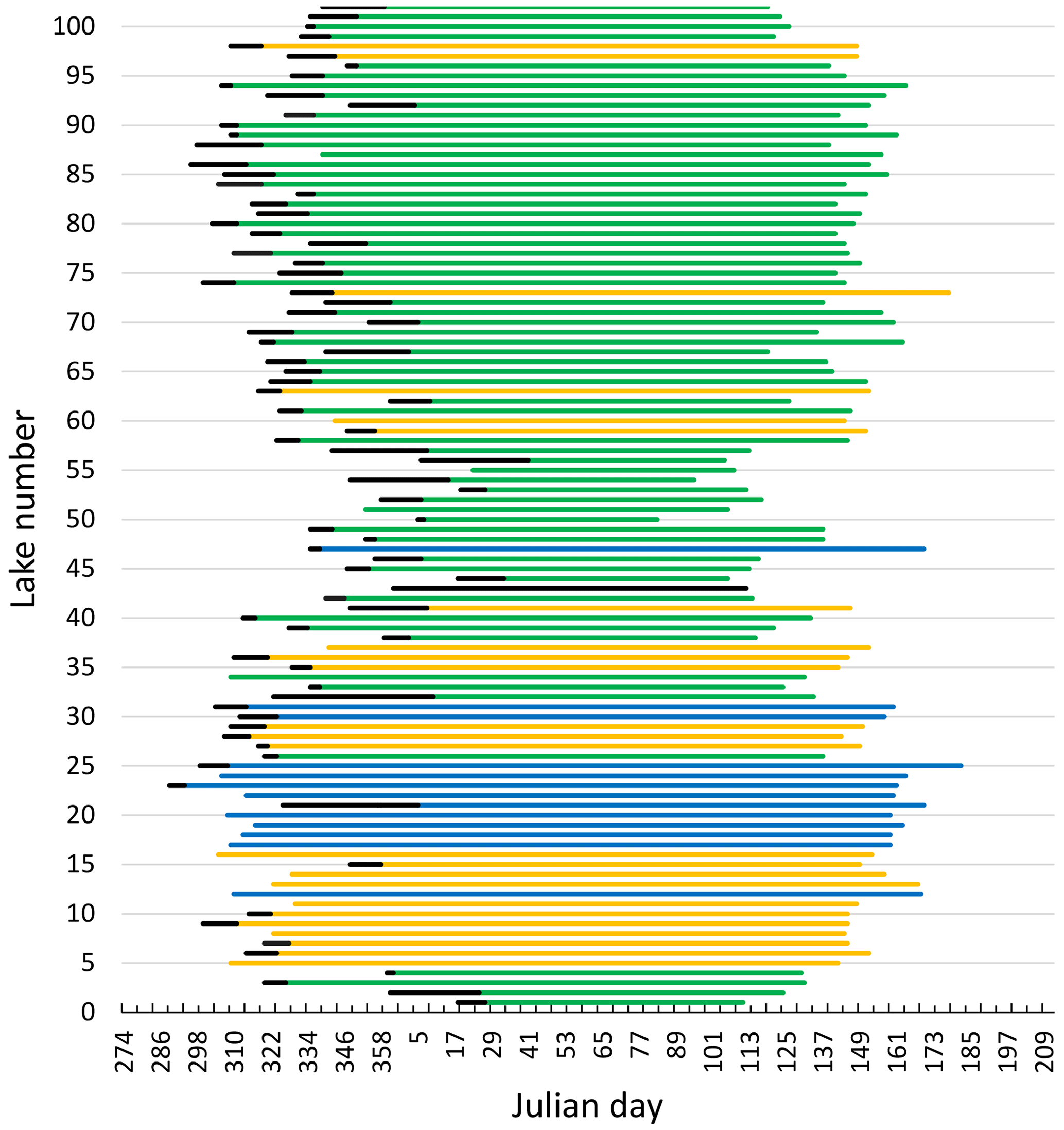
Figure 3 Median date of freeze-up (black line), frozen lake and break-up (coloured lines) for 101 Norwegian lakes during 1890–2020. The x axis starts at 274 (1 October) and ends at 212 (31 July). The colour indicates elevation for each lake (green: < 500 m a.s.l.; yellow: 500–1000 m a.s.l.; blue: > 1000 m a.s.l.). For information on each lake see Appendix A and B.

Table 1 Correlation between timing of ice break-up, lake freeze-up, time when the lake was completely frozen and length of ice-free period for 101 Norwegian lakes. All correlation coefficients are significant at P<0.001.

3.1 Spatial variation in average ice phenology

We tested for drivers of variation in average time of ice break-up, lake freeze-up, time when a lake is completely frozen over and the length of the ice-free period. A summary of the model selection results is presented in Appendix D.

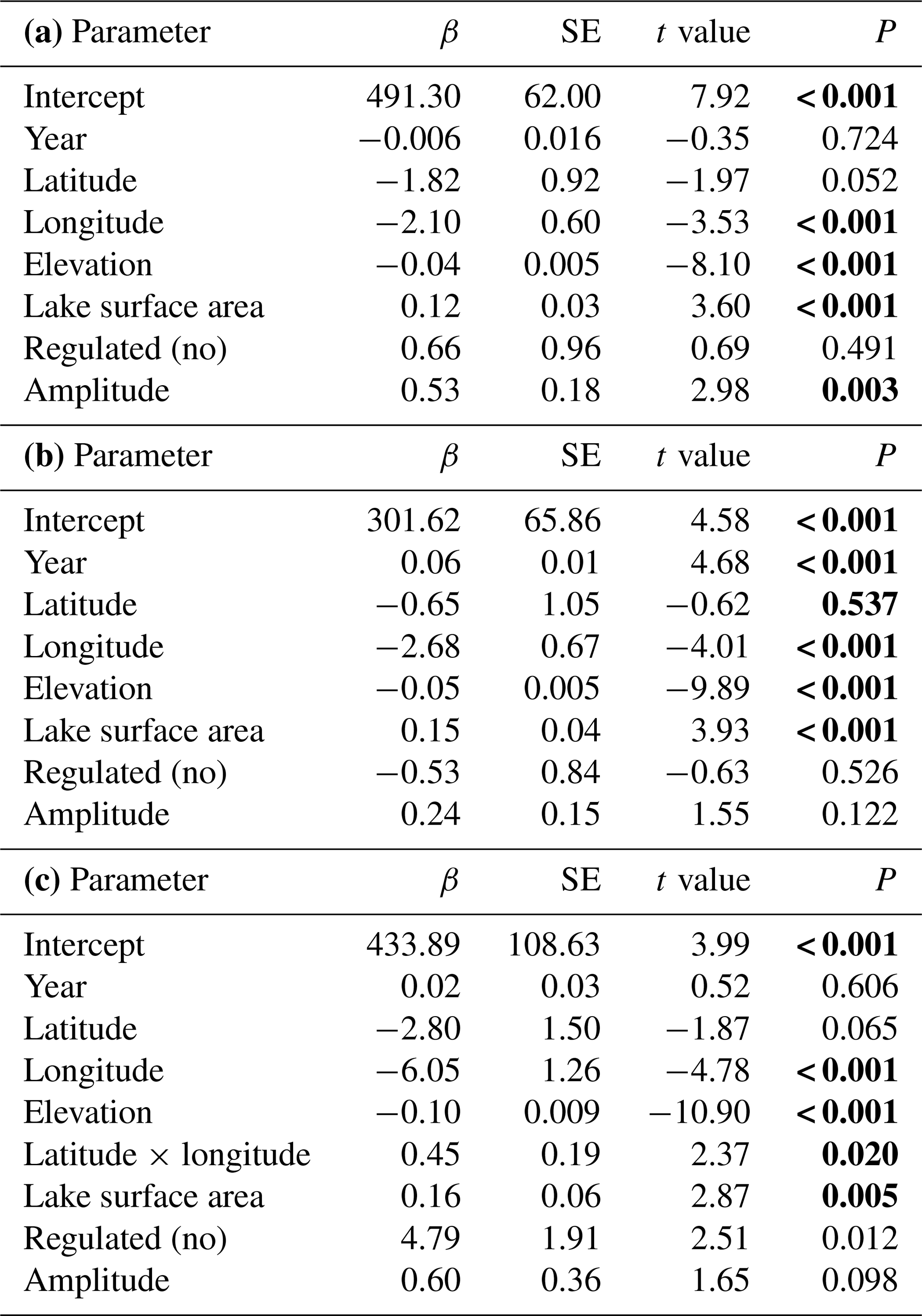
The spatial variation in average time of ice break-up was best explained by a complex model including a three-way interaction between latitude, longitude and elevation (Table 2). The best model did, however, include a weak negative effect of annual inflow to the lake, but not distance to the sea. Distance to sea was, however, included in a model within 0.4 AIC_c units of the best model. There were only small effects of the various lake characteristics, but ice break-up was later with increasing latitude (2.3 d per ^∘ N), longitude (1.5 d per ^∘ E) and elevation (3.4 d per 100 m) (Fig. 4). The lakes are situated geographically such that latitude and longitude are strongly positively correlated (r=0.825, p<0.001), longitude and elevation are negatively correlated ($r=-\mathrm{0}$.404, p<0.001), and latitude and coastal distance are negatively correlated ($r=-\mathrm{0}$.479, p<0.001), indicating that the effects should be interpreted with caution. Furthermore, there was large within-lake variability in timing of ice break-up (Table 3), with an average coefficient of variation (CV; defined as standard deviation divided by the mean) of 8.90 %. Within-lake CV was negatively correlated with latitude, longitude, elevation and distance to the coastline. This indicates larger phenological variation in lakes in southern and western areas and at lower elevation.

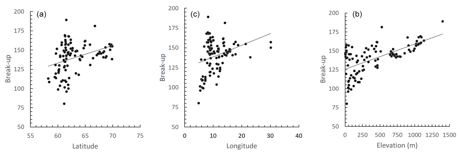
Figure 4 The correlation between the average timing of ice break-up and latitude, longitude and elevation of 101 Norwegian lakes during the period 1890–2020. The lines represent best linear fit. (a) r=0.345, p<0.001. (b) r=0.329, p<0.001. (c) r=0.630, p<0.001.

Table 2 Model summary. Testing for temporal variation in time of ice break-up, time of lake freeze-up, time when the lake is completely frozen, and length of ice-free period for 99 lakes in Norway. Parameter estimates for the best model are given (see Appendix Table A1 for results from the model selection). Significant parameter estimates are given in bold. (a) Time of ice break-up: summary statistics with parameter estimates (β± SE), t values and significance level (P). Model F ratio = 91.46 (d.f. = 8, 92), total N=101, P<0.0001, R²=0.888. (b) Time of lake freeze-up: summary statistics with parameter estimates (β± SE), t values and significance level (P). Model F ratio = 23.14 (d.f. = 6, 80), total N=87, P<0.0001, R²=0.634. (c) Time when lake is completely frozen: summary statistics with parameter estimates (β± SE), t values and significance level (P). Model F ratio = 42.57 (d.f. = 3, 96), total N=100, P<0.0001, R²=0.570. (d) Length of ice-free period: summary statistics with parameter estimates (β± SE), t values and significance level (P). Model F ratio = 34.06 (d.f. = 6, 80), total N=87, P<0.0001, R²=0.719.

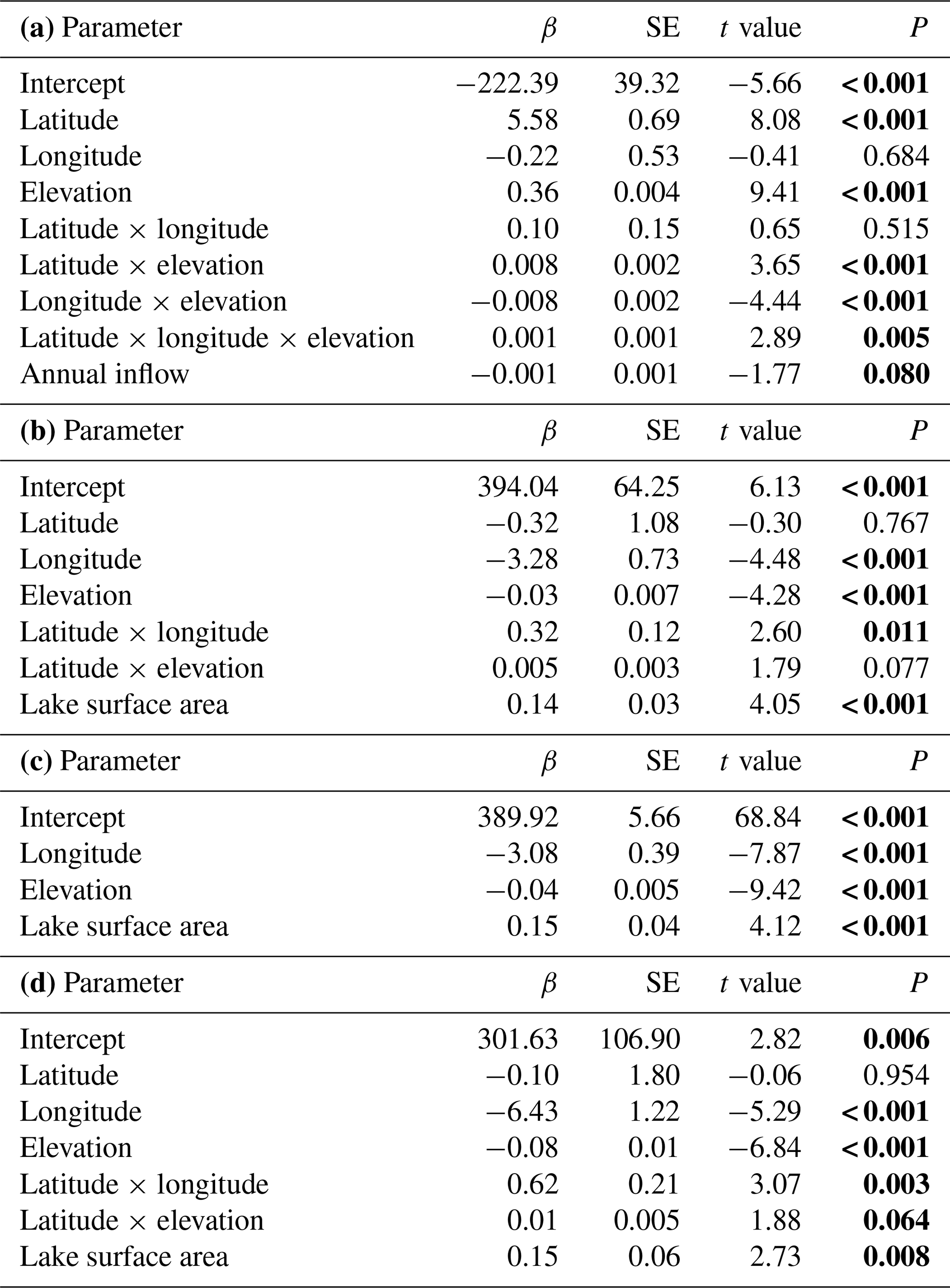
The best models explaining variation in the timing of lake freeze-up, time when the lake is completely frozen, and the length of the ice-free period usually contained an interaction effect between longitude and elevation. All models also included a positive effect of lake surface area (Table 2, Appendix C). Overall, lakes freeze-up earlier and have a shorter ice-free period with increasing longitude and elevation. Large lakes also take longer to freeze and were ice-free for longer than smaller lakes. The within-lake variation in timing of freeze-up (mean CV = 4.45 %) and when the lake was completely frozen (mean CV = 4.55 %) was less than the variation in the length of the ice-free period (mean CV = 15.04 %). The CV of these three phenological traits was negatively correlated with elevation and coastal distance (Table 3). The effect of longitude was more variable.

Table 3 Summary statistics for the coefficient of variation (mean, median and range), as well as correlation between coefficient of variation (CV) and various geographic traits for each lake (elevation, latitude, longitude and distance to the coastline).

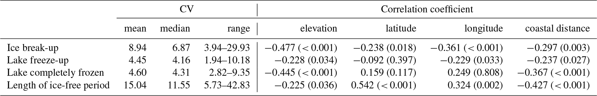
Table 4 Testing for temporal variation in time of lake freeze-up, time when the lake is completely frozen and length of ice-free period for 99 lakes in Norway. Lake identity is modelled as a random factor, and year is always included in the model as a fixed effect. Summary statistics with parameter estimates (β± SE), t values and significance level (P) for the best model are given (see Appendix Table B1 for results from the model selection). Significant parameter estimates are given in bold. (a) Timing of lake freeze-up: total N=3035, R²=0.676, P<0.0001. The random lake effect accounts for 44.0 % of total variance. (b) Time when lake is completely frozen: total N=4084, R²=0.697, P<0.0001. The random lake effect accounts for 50.6 % of total variance. (c) Length of ice-free period: total N=2807, R²=0.663, P<0.0001. The random lake effect accounts for 34.4 % of total variance.

3.2 Temporal variation in timing of lake freeze-up, time when the lake is completely frozen and length of ice-free period

The best models, based on the AIC_c criterion, for timing of lake freeze-up, time when the lake was completely frozen and the length of the ice-free period contained geographic parameters such as elevation, latitude and longitude (Appendix D). Lake surface area also had a positive effect on all these three phenological traits. In addition, lake regulation and the amplitudinal range in water level had an impact on all traits. There was little temporal variation in these traits on the long timescale analysed here; only for when the lake was completely frozen over did we find a significant (p<0.001) positive temporal trend, indicating that the lakes are completely frozen later in the autumn in recent years (Table 4).

3.3 Temporal trends in timing of ice break-up

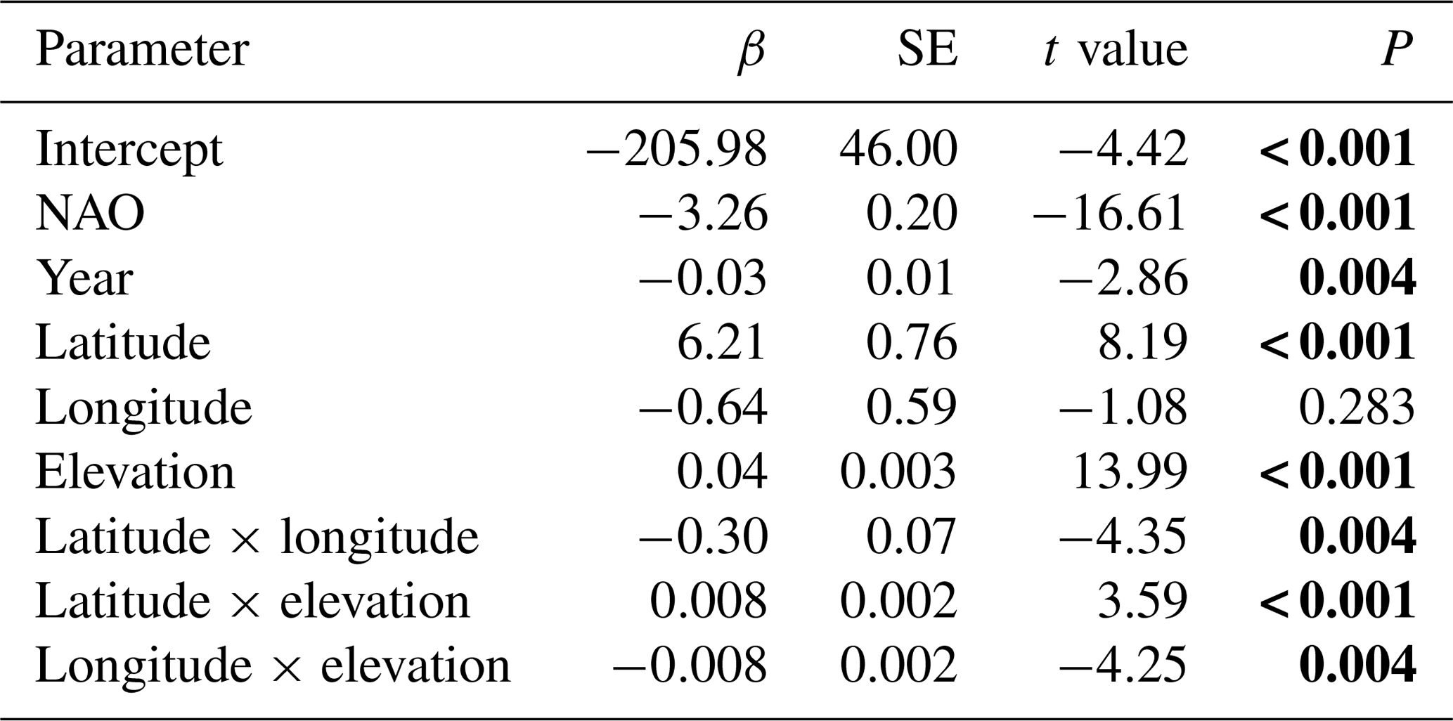
The best model for the timing of ice break-up included the effects of geography, time and climate (Appendix E). Ice break-up occurred later during spring with increasing elevation, latitude and longitude. These effects are complex, as indicated by the various significant interaction effects. In addition, there was a significant negative temporal trend in ice break-up; i.e. ice break-up occurred earlier in the spring (Table 5). There was also a significant climate effect, with a negative linear effect of the NAO (p<0.001).

Table 5 Model summary. Temporal and climate effects on in time of ice break-up for 98 lakes in Norway. Lake identity is modelled as a random factor, and year is always included in the model as a fixed effect. NAO is included as the climate effect. Summary statistics with parameter estimates (β± SE), t values and significance level (P) for the best model are given (see Appendix Table C1 for results from the model selection). Significant parameter estimates are given in bold. Total N=4194, R²=0.726, P<0.0001. The random lake effect accounts for 22.3 % of total variance.

3.4 Non-linear temporal trends in ice phenology

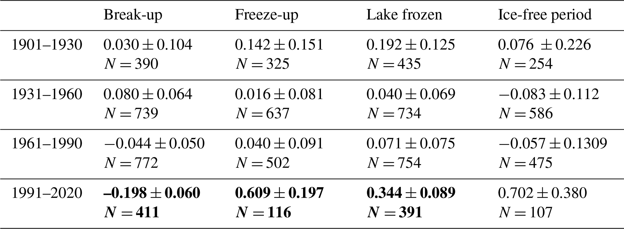
Many studies indicate that climate has been changing faster during recent decades. To investigate for potential non-linear trends in ice phenology we analysed for temporal trends within four different time periods (1901–1930, 1931–1960, 1961–1990, 1991–2020). We selected 35 lakes with relatively long and continuous data series exceeding 50 years for both date of break-up and date of completely frozen lake (Appendix F). We used a period-specific mixed model, assuming similar temporal trends (slopes) for all lakes (random intercept only). During the three first time periods none of the slope estimates were significant (Fig. 5, Table 6), whereas during the last time period (1991–2020) most temporal trends were significant. During this period ice break-up happened approximately 2 d earlier per decade, whereas time of ice freeze-up and time when lake is completely frozen were on average 6 and 3 d later per decade. Furthermore, the length of the ice-free period has become 7 d longer per decade, although this effect was marginally non-significant (p=0.068).

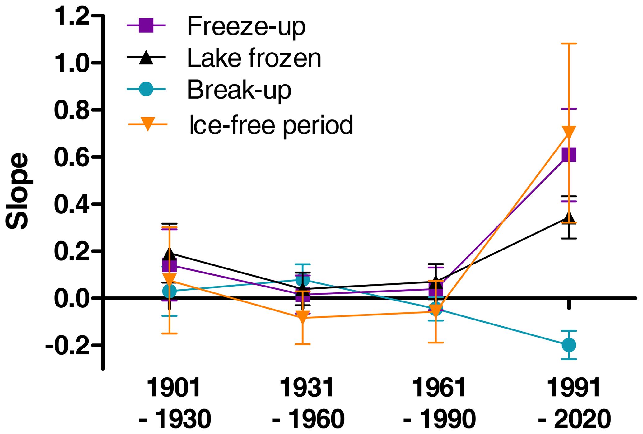
Figure 5 Estimated slopes from general linear mixed models with aspects of ice phenology as response variables (parameter estimates and significance level are given in Table 6). Means and standard error are given.

Table 6 Parameter estimates (slope ± SE) from general linear mixed models with ice phenology estimates as response variables, year as predictor and lake identity as random effect. The time series are sorted into 30-year periods (1901–1930, 1931–1960, 1961–1990, 1991–2020). Significant estimates are given in bold. The lakes included are given in Appendix G.

4 Discussion

Our analysis of ice phenology of 101 Norwegian lakes covering the period from the 1890s to 2020 gave two major results. Firstly, the analysis indicated significant trends in ice phenology in recent years. Ice break-up occurred earlier, ice freeze-up and completely frozen occurred later, and all trends were accelerating. This results in a longer ice-free season. Secondly, the coefficient of variation in the different ice phenology variables was larger in lakes in southern and western areas and at lower elevation, indicating that lakes in these areas are most influenced by climate change.

4.1 Geographical parameters

The investigated lakes cover a range of climatic zones in a latitudinal, longitudinal and elevational perspective. These variables clearly showed complex and significant interactions, especially for ice break-up, indicating the problems in illuminating the individual importance of the geographical parameters. The date of break-up generally occurs later with increasing latitude, modified by macroscale to local-scale atmospheric circulation and lake characteristics (Blenckner et al., 2004; Livingstone et al., 2009). Our results support this latitudinal trend, but we also found that longitude, elevation and lake size had significant effect.

Ice break-up dates are shown to be 2.3 d later with each degree of higher latitude. This is considerably less than previously documented in Fennoscandia (3.3–5.4 d per ^∘ N) (Efremova et al., 2013; Blenckner et al., 2004) and in North America 3.5 d per ^∘ N (Williams et al., 2006). There is no obvious reason for this difference. One possible explanation could be that registration of ice parameters differs both within and between studies. Moreover, the oceanic effect could modify the relationship as the majority of lakes in northern Norway are situated close to the ocean in contrast to the southern lakes that are mostly continental.

Moreover, we found that ice break-up was delayed 3.4 d by a 100 m increase in elevation. This is also slightly lower than in Karelian lakes, where Efremova et al. (2013) found a delay of 5 d per 100 m. Although there is considerable climatic difference between Norway and Karelia as Karelian lakes in general experience a more continental climate, the Karelian lakes also cover less variation in elevation.

Although several studies have investigated ice phenology in Europe, most of them have not included longitude in their analyses. One reason could be the complexity of the parameter. In contrast to latitude, which reflects insolation received, longitude reflects more the distance from the coast. However, one exception is the study of Polish lakes by Wrzesinski et al. (2015). The lakes are situated in the northern region and covered a wide longitudinal range (14–24^∘ E), although a somewhat smaller range compared to the Norwegian lakes. Wrzesinski et al. (2015) found that break-up increased by 1 d per ^∘ E, compared to 1.5 d per ^∘ E in our study. The location of the Polish lakes indicates that any effect of the Baltic Sea is similar. In contrast, in Norway the climate becomes more continental when moving eastwards, especially south of 61^∘ N where the mountain chain that runs north–south creates a distinct difference in climate from west to east. Thus, the longitudinal effect could as well be due to the climatic conditions as the proximity to the ocean renders the climate milder in the west. The longitudinal effect should therefore be treated with caution. However, the global study by Sharma et al. (2019) showed that distance to the coast was important in determining whether lakes had annual winter ice cover. In our analysis the distance from ocean did not per se have any significant effect of any of the ice phenology parameters.

Our results demonstrated a complex relationship among geographical parameters describing date of freeze-up. The best models explaining variation in the timing of lake freeze-up contained an interaction effect between longitude and elevation, in addition to a positive effect of lake surface area. This differs from the results from other studies in the region. The Karelian lakes, covering 54–68^∘ N, freeze up 2.3 d earlier for every degree of increasing latitude (Efremova et al., 2013), while Swedish (58–68^∘ N) and Finnish (61–69^∘ N) lakes freeze up 2.8 and 4.5 d earlier for each degree of increasing latitude, respectively (Blenckner et al., 2004). The most obvious explanation for this discrepancy is due to altitudinal variation. The Norwegian lakes cover 1400 m in elevation range, whereas the lakes in Karelia are all situated lower than 204 m, in Sweden lower than 340 m and in Finland lower than 473 m. An additional complicating factor is the oceanic climate that, if anything, is more pronounced for Norwegian lakes than lakes in Sweden, Finland and Karelia.

In our model, distance from the coast significantly contributes neither to freeze-up nor break-up date, probably as distance to the coast was included both in the latitude and longitude variables. This is in contrast to the analyses of 41 Finnish lakes where a pronounced deflection of isolines of both freeze-up and break-up date northward near the Baltic Sea coast was documented (Palecki and Barry, 1986; Korhonen, 2006).

The predictable seasonal cycle in solar radiation is characteristic of higher latitudes. Weyhenmeyer et al. (2011) hypothesised, based on a global dataset, that lakes north of 61^∘ N had lower inter-annual variability in seasonal cycle than lakes at latitudes lower than 61^∘ N. The Norwegian lakes are distributed along a latitudinal gradient to test this hypothesis in a robust way. Our results lend support to this, as the within-lake coefficient of variation (CV) of ice break-up, freeze-up and length of ice-free season was negatively correlated with latitude, longitude, elevation and/or distance to coastline. This indicates larger phenological variation in lakes in southern and western areas and at lower elevation.

4.2 Temporal trends

Although many studies have documented trends in ice phenology, few studies have investigated changes across specific periods to elucidate periods with stronger trends. In a study of global datasets Benson et al. (2012) and Newton and Mullan (2020) showed that trends in ice variables were steeper over the last 30-year period. Similar increases in trends in the last 2 decades have been shown for Karelian lakes (Efremova et al., 2013) and the Great Lakes region (Mishra et al., 2011).

Our analyses revealed significant, accelerating trends for earlier break-up, later freeze-up and lately completely frozen lakes after 1991. Moreover, the trend for a longer ice-free period also accelerated during this period, although the trend was not significant. These trends are in accordance with an increase in air temperature in the spring and autumn, as well for the global temperature over the last decades (Benson et al., 2012; Hansen et al., 2006). Our results are in accordance with Newton and Mullan (2020), showing marked differences in ice phenology in Fennoscandian lakes (Sweden, Finland) across 30-year periods after 1931. Newton and Mullan (2020) found that break-up appeared to be earlier and trends more pronounced in southern regions during the first period. In the next period, 1961–1999, break-up trends increased in magnitude, and the lakes with negative trends in the previous period shifted to be positive. In the last period, the strength of the trends in earlier break-up increased and reached 3.9 d per decade. In our study, the trend in the 1991–2020 was 2.0 d per decade. Korhonen (2006) also showed a significantly earlier break-up of 6–9 d over a hundred years for Finnish lakes, although the data were not analysed in 30-year periods. One plausible reason for a slower trend in Norwegian lakes during this period than in the rest of Fennoscandia is the influence of the ocean. There has been considerable change in the 0 ^∘C isotherm with a marked reduction in the area below 0 ^∘C (see Fig. 6). The change is recorded throughout Norway but at a larger scale in the continental areas between 61 and 63^∘ N. A significant correlation between break-up and 0 ^∘C isotherm has been documented for Arctic lakes in North America, Europe and Siberia (Šmejkalova et al., 2016). The extension of the Gulf Stream, the North Atlantic Drift, along the Norwegian coast contributes to a mild climate and reduced climate. The speed of thermal change in the ocean is less rapid and less variable than in inland waters (Woolway and Maberly, 2020).

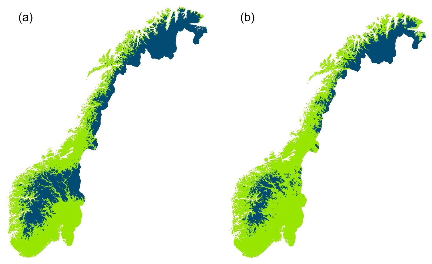
Figure 6 Areal maps of the annual mean air temperature below 0 ^∘C (dark colour) in 1961–1990 (a) and 1991–2020 (b) (https://rmets.onlinelibrary.wiley.com/doi/full/10.1002/qj.3208, last access: 5 March 2021).

Changes in ice phenology depend on several climatic forcing variables, such as air temperature, solar radiation, wind and snowfall (Magnusson et al., 1997). A significant increase in global air temperature during the last century is well documented (e.g. Hansen et al., 2006; Robinson, 2020). Newton and Mullan (2020) showed that rising temperature appears to be the dominant factor for the shift towards earlier break-up and later freeze-up in the Northern Hemisphere. Precipitation may also play a role in the observed trends. Nordli et al. (2007) found a significant correlation (R²=0.58) between date of break-up in lake Randsfjorden and the mean temperature in February to April. Duguay et al. (2006) showed that trends towards later freeze-up corresponded with areas of increasing autumn snow cover and that spatial trends in break-up were consistent with changes in spring snow cover duration. Similarly, Jensen et al. (2007) in a study of ice phenology trends across the Laurentian Great Lakes region found that variability in the strength of trends in earlier break-up was partly explained by number of snow days or snow depth. For the lake Litlosvatn, in the mountain area of western Norway, Borgstrøm (2001) found a clear relationship between spring snow depth and the date on which the lake was free of ice. The altitudinal gradient causes considerable regional difference in annual precipitation in Norway (Hanssen-Bauer, 2005). The general trend in increasing temperature and precipitation observed from 1875 to 2004 has been modelled to increase to 2100, although there will be regional differences (Hanssen-Bauer et al., 2017). Thus, our results concerning the recent trends in ice phenology probably indicate a new situation for ice formation in Norwegian lakes. However, this is in agreement with a general trend in the Northern Hemisphere shown by an increase in extreme events for lake ice (Filazzola et al., 2020).

Biological consequences

Shifts in ice phenology have major repercussions for the biota of lakes and rivers (Prowse, 2001; Prowse et al., 2011; Caldwell et al., 2020), as ice cover changes the aquatic environment, in terms of not only light penetration, but also the physical characteristics of the environment such as temperature. Of special interest is that the trend in earlier ice break-up and the loss of ice will stimulate biological production. In late autumn, solar insulation is restricted, and thus a prolonged period without ice has limited consequences for aquatic production. Caldwell et al. (2020) tested a conceptual model that expressed how earlier break-up affected aquatic ecosystems. The effect differed between and within tropic levels. Whereas contrasting effects were found between littoral and pelagic zooplankton production, the modelled brook trout (Salvelinus fontinalis) did not profit from the increased zooplankton production and experienced reduced fitness. A review of the long-term dynamics of fish species in Europe (Jeppesen et al., 2012) revealed a shift towards higher dominance of eurythermal species. Loss of ice cover increased resting metabolism by approximately 30 % in an Atlantic salmon (Salmo salar) population (Finstad et al., 2004), and the recruitment of an alpine brown trout (Salmo trutta) population was strongly affected by accumulated snow depth and thereby the timing of ice-break (Borgstrøm and Museth, 2005). Moreover, the outcome of competition in sympatric populations of brown trout and Arctic charr (Salvelinus alpinus) is strongly dependent on the duration of ice-cover as high charr abundance is correlated with low trout population growth rate only in combination with long winters (Helland et al., 2011). In addition, aquatic insects, such as Ephemeroptera and Plecoptera, may change their voltinism and their emergence timing in a warmer climate (Brittain 1978, 2008; Sand and Brittain 2009). We still have limited knowledge about how climate change in general may have impacts on arctic and alpine fishes and fish populations (Reist et al., 2006). This is also the case with changes in ice phenology. The biological consequences of changes in ice phenology will occur first and be most marked in lakes with high coefficient of variation in the ice phenology parameters, that is, in lakes situated in the coastal lowlands, in the southernmost part, and in the eastern part of southern Norway. We suggest that biological consequences will be small in these areas as ubiquitous species with wide environmental limits often dominate, although those species dependent on regular ice conditions will be replaced by species with a more flexible life history (Brittain, 2008; Brittain et al., 2020). In the long-term this replacement is also likely to occur in lakes at higher elevation as ice cover duration decreases and becomes more variable at the same time as winter temperature increases.

5 Conclusions

Ice phenology is complex and determined by the interaction of a range of parameters. This study shows that elevation, latitude and longitude all significantly affect ice phenology in Norwegian lakes. Overall, the length of ice-free season becomes longer with increasing values of each parameter. Lake characteristics are of minor importance, although lake size had a significant effect. In addition, a significant temporal effect of changing climate was detected during 1991–2020 but not in the three earlier 30-year periods. During this latter period ice break-up happened approximately 2 d earlier per decade, whereas timing of ice freeze-up and time when lakes are completely frozen was on average 6 and 3 d, respectively, later per decade. Furthermore, the length of the ice-free period has become 7 d longer per decade. These trends are shown to happen concomitantly with a considerable reduction in the area with annual mean air temperature below 0 ^∘C. The reduction is most pronounced in continental areas between 61 and 63^∘ N. An understanding of the relationship between ice phenology and geographical and climate parameters is a prerequisite for predicting the potential consequences of climate change on ice phenology and lake biota.

Appendix A

Table A1 Lake characteristics of the 101 Norwegian lakes used in the analyses. “Regulated” shows the year when the lake was developed for hydropower, and the figure in the brackets is the annual water level amplitude; “no” indicates a pristine lake.

Appendix B

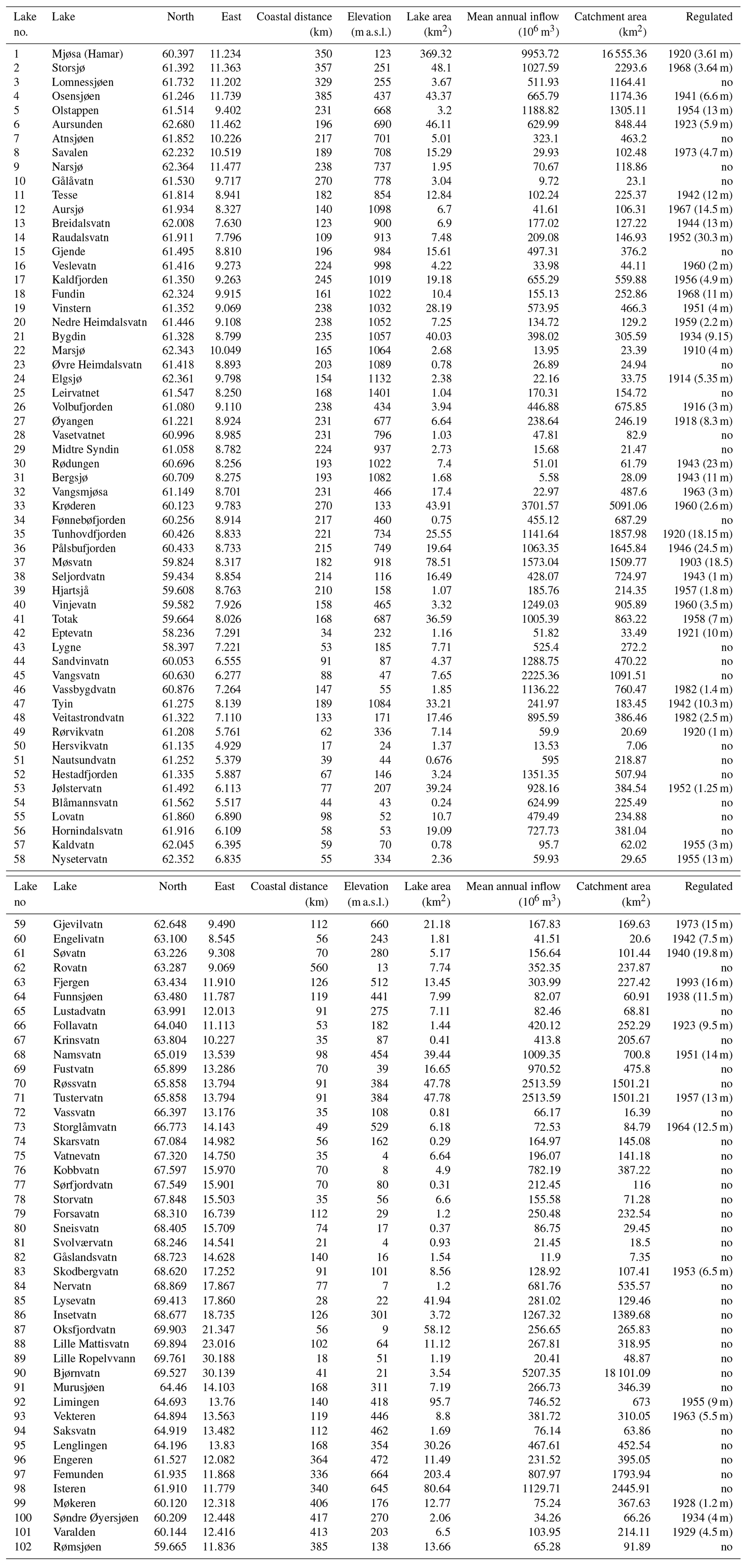
Table B1 Summary of ice phenology recordings from 101 Norwegian lakes. Minimum and maximum recordings are given in brackets.

Appendix C

Table C1 Variation in average time of ice break-up, time of lake freeze-up, time when lake is completely frozen, and length of ice-free period. The full model is formulated as follows (see description of parameters in the main text): $Y=\mathit{\mu }+{\mathit{\alpha }}_{\mathrm{1}}$Ele +α₂ Lat +α₃ Long +α₄Ele × Lat +α₅ Ele × Long + α₆Long × Lat +α₇ Ele × Long × Lat +α₈Distance +α₉Area +α₁₀Catch + α₁₁Flow +ε. Selection of the best model was based on AIC. The full model and the three best models are presented, with the best model given in bold. AIC and ΔAIC are given. (a) Time of ice break-up. (b) Time of lake freeze-up. (c) Time when lake is completely frozen. (d) Length of ice-free period.

Appendix D

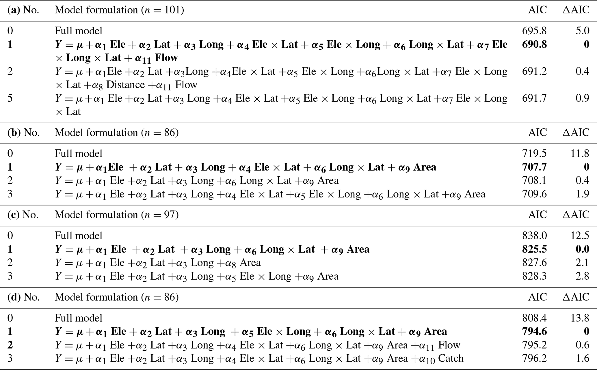
Table D1 Test for temporal variation in time of lake freeze-up, time when lake is completely frozen, and length of ice-free period for 98 lakes in Norway. Lake identity is modelled as a random factor, and year is always included in the model as a fixed effect. The full model is formulated as follows (see description of parameters in the main text): $Y=\mathit{\mu }+{\mathit{\alpha }}_{\mathrm{1}}$ Ele +α₂ Lat +α₃ Long +α₄ Ele × Lat +α₅ Ele × Long + α₆ Long × Lat +α₇ Ele × Long × Lat +α₈ Distance +α₉ Area +α₁₀ Catch + α₁₁ Flow +α₁₂ Year +α₁₃ Regulated +α₁₄ Amplitude +ε. Selection of the best model was based on AIC. The full model and the three best models are presented, with the best model given in bold. AIC and Δ AIC are given. (a) Time of lake freeze-up. (b) Time when lake is completely frozen. (c) Length of ice-free period.

Appendix E

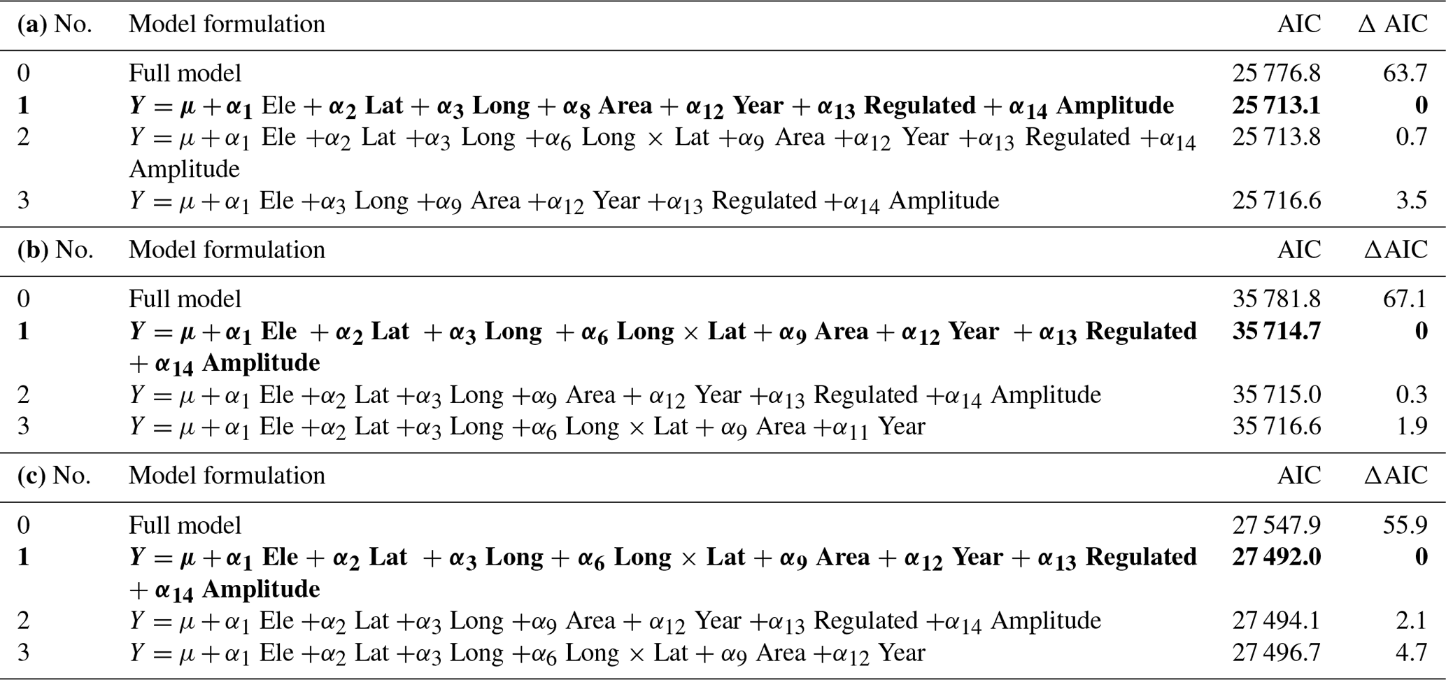
Table E1 Test for temporal variation in time of ice break-up. Lake identity is modelled as a random factor, and year is always included in the model as a fixed effect. NAO is included in the model as both a linear and a non-linear effect. The full model is formulated as follows (see description of parameters in the main text): $Y=\mathit{\mu }+{\mathit{\alpha }}_{\mathrm{1}}$ Ele +α₂ Lat +α₃ Long +α₄ Ele × Lat +α₅ Ele × Long + α₆ Long × Lat +α₇ Ele × Long × Lat +α₈ Distance +α₉ Area +α₁₀ Catch + α₁₁ Flow +α₁₂ Year +α₁₃ Regulated +α₁₄ Amplitude +α₁₅ NAO +α₁₆ NAO²+ε. Selection of the best model was based on AIC. The full model and the three best models are presented, with the best model given in bold. AIC and Δ AIC are given.

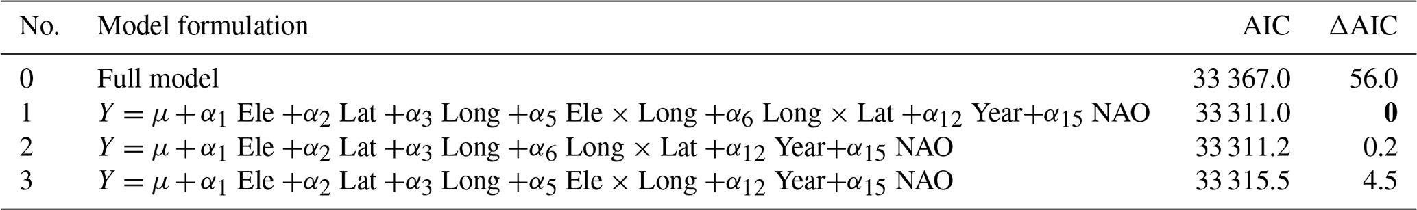
Table E2 Test for non-linear temporal trends in ice phenology in 30-year periods. Lakes with > 50 years of records of both date of break-up and date of frozen lake.