Simulated Ka- and Ku-band radar altimeter height and freeboard estimation on snow-covered Arctic sea ice

Owing to differing and complex snow geophysical properties, radar waves of different wavelengths undergo variable penetration through snow-covered sea ice. However, the mechanisms influencing radar altimeter backscatter from snow-covered sea ice, especially at Ka- and Ku-band frequencies, and the impact on the Ka- and Ku-band radar scattering horizon or the “track point” (i.e. the scattering layer depth detected by the radar re-tracker) are not well understood. In this study, we evaluate the Ka- and Ku-band radar scattering horizon with respect to radar penetration and ice floe buoyancy using a first-order scattering model and the Archimedes principle. The scattering model is forced with snow depth data from the European Space Agency (ESA) climate change initiative (CCI) round-robin data package, in which NASA's Operation IceBridge (OIB) data and climatology are included, and detailed snow geophysical property profiles from the Canadian Arctic. Our simulations demonstrate that the Ka- and Ku-band track point difference is a function of snow depth; however, the simulated track point difference is much smaller than what is reported in the literature from the Ku-band CryoSat-2 and Ka-band SARAL/AltiKa satellite radar altimeter observations. We argue that this discrepancy in the Ka- and Ku-band track point differences is sensitive to ice type and snow depth and its associated geophysical properties. Snow salinity is first increasing the Ka- and Ku-band track point difference when the snow is thin and then decreasing the difference when the snow is thick (>0.1 m). A relationship between the Ku-band radar scattering horizon and snow depth is found. This relationship has implications for (1) the use of snow climatology in the conversion of radar freeboard into sea ice thickness and (2) the impact of variability in measured snow depth on the derived ice thickness. For both (1) and (2), the impact of using a snow climatology versus the actual snow depth is relatively small on the radar freeboard, only raising the radar freeboard by 0.03 times the climatological snow depth plus 0.03 times the real snow depth. The radar freeboard is a function of both radar scattering and floe buoyancy. This study serves to enhance our understanding of microwave interactions towards improved accuracy of snow depth and sea ice thickness retrievals via the combination of the currently operational and ESA's forthcoming Ka- and Ku-band dual-frequency CRISTAL radar altimeter missions.

1 Introduction

Since 2010, basin-scale Arctic sea ice thickness (H_I) has been estimated monthly during the winter season using the European Space Agency's CryoSat-2 Ku-band frequency radar altimeter data (e.g., AWI https://www.meereisportal.de/en/, last access: 29 March 2021; CPOM http://www.cpom.ucl.ac.uk/csopr/seaice.php, last access: 29 March 2021; and NSIDC, https://nsidc.org/data/RDEFT4, last access: 29 March 2021) and using joint French Aerospace Agency/Indian Space Research Organization's Ka-band SARAL/AltiKa radar altimeter data (e.g., Maheshwari et al., 2015). Neither CryoSat-2 nor AltiKa directly measure H_I. Instead, they provide a measure of the sea ice freeboard (F_I) – the height of the sea ice floe from the local sea level, measured in either leads or cracks located adjacent to the floe. To convert F_I to H_I, hydrostatic equilibrium is assumed (Laxon et al., 2003). This assumption requires geophysical property information on the overlying snowpack, as well as the underlying sea ice, which can affect the accuracy of the radar height estimate. These geophysical parameters include snow depth, snow density, temperature, salinity, snow grain size, snow surface–sea-ice interface roughness, sea ice density, and seawater density (Landy et al., 2020; Nandan et al., 2020; Landy et al., 2019; Tonboe et al., 2010; Nandan et al., 2017a; Alexandrov et al., 2010; Ricker et al., 2014). The radar height estimate or track point is conceptualized as the scattering surface depth detected by the radar re-tracker algorithm and the floe buoyancy, and in turn it impacts the accuracy of F_I and H_I estimates (Ricker et al., 2014). The track point represents the return radar echo waveform measured by a radar altimeter, which is then statistically analyzed in the re-tracker algorithm to extract information on the scattering surface depth between the air–snow interface and a physical interface either within the snowpack volume, at the snow–sea-ice interface, or within the sea ice volume (e.g., Kwok and Kacimi, 2018). However, the detected horizon may not coincide with a physical interface. That is why we prefer to call it the “track point”. The re-tracker algorithm that we are using can be tuned so that the radar height estimate coincides with the snow–sea-ice interface. However, satellite radar backscatter interactions are non-linear, and the total backscatter is dominated by a relatively small areal fraction of plane facets on the surface (Fetterer et al., 1992; Ulander and Carlström, 1991). Also, thinner ice types within the radar footprint exhibit higher backscatter than thicker sea ice because of differences in surface roughness, leading to oversampling of the thinner ice types and undersampling of the thicker ice types (Tonboe et al., 2010; Aldenhoff et al., 2019). In other words, the radar scattering is dominated by an area which is only a fraction of the total surface and bulk snow and ice properties that are relevant for the buoyancy of the floe and may not be representative of the scattering parts of the floe. This has implications for snow–sea-ice field sampling strategy and how snow depth and ice thickness and density are used in the processing of radar altimeter data for deriving H_I. When deriving H_I, snow depth, snow, ice, and water density, and radar penetration are accounted for in the processing of the sea ice thickness products from CryoSat-2. During the F_I-to-H_I conversion and if the snow depth is known, there are two corrections involving snow: (1) there is a radar penetration correction that will compensate for this sensitivity and locate the scattering horizon at the snow–sea-ice interface (Kwok et al., 2011; Ricker et al., 2014; Mallett et al., 2020; Stroeve et al., 2020), and (2) there is a correction to the ice floe buoyancy as a function of snow depth.

Several studies suggest that it may be possible to derive snow depth directly using a dual-frequency approach by combining Ka- and Ku-band radar altimetry (e.g., Lawrence et al., 2018; Guerreiro et al., 2016). The underlying principal behind this technique is that the assumption of predominant Ka-band scattering originates at the air–snow interface, while for Ku-band, the dominant scattering originates at the snow–sea-ice interface (Beaven et al., 1995; Lawrence et al., 2018; Laxon et al., 2013; Kurtz et al., 2014). Armitage and Ridout (2015) compared the effective scattering surface of the Ka-band altimeter AltiKa and Ku-band CryoSat-2 to the snow depth and snow surface measurements from NASA's Operation IceBridge (OIB) campaigns. They found that the AltiKa dominant radar height is 0.54 times the snow depth above the ice surface using the OIB Quick Look snow depth product. They also found that the CryoSat-2 radar height was deeper into the snow volume, well below the Ka-band radar height but still above the snow–sea-ice interface, and that the depth of this horizon was dependent on sea ice type. Observed AltiKa and CryoSat-2 mean freeboard differences were found to be ∼0.04 to 0.07 m from October to March (Fig. 2 in Armitage and Ridout, 2015). Lawrence et al. (2018) indicated that some of these differences between AltiKa and CryoSat-2 could be attributed to the different re-tracker algorithms used in the processing scheme of the two datasets.

While Guerreiro et al. (2016) found that Ka-band radar scattering primarily originates from the air–snow interface, based on simple modeling assumptions, Maheshwari et al. (2015) assumed the effective Ka-band scattering interface was coincident with the snow–sea-ice interface in their derivation of sea ice freeboard using AltiKa. Seasonally evolving snow covers with internal density layering (e.g., compacted wind slabs), ice lenses, melt–refreeze layers, brine-wetting (only on first-year sea ice, FYI), and large spatial diversity add to the geophysical complexity and manifest vertical shifting of the Ku-band radar height by several or more centimeters above the snow–sea-ice interface (Nandan et al., 2020, 2017a; Tonboe et al., 2006a). This significantly impacts the accuracy of F_I and H_I retrievals from radar altimetry both in the Arctic and in the Antarctic (Nandan et al., 2020; Kwok and Kacimi, 2018; Ricker et al., 2014, 2015; Kwok, 2014; Hendricks et al., 2010). This ambiguity and inconsistency in assumptions and previous study results suggest detailed investigation into the location of the Ka- and Ku-band radar height for snow-covered sea ice is warranted.

In this study, we simulate the combined effect of snow depth and density on the Ka- and Ku-band radar height and on the sea ice floe buoyancy. To achieve our research objective, we use a first-order radar scattering model, together with a reference snow depth and density dataset from the European Space Agency (ESA) climate change initiative (CCI) round-robin data package program, to describe any potential variability in Ka- and Ku-band radar height in snow-covered Arctic sea ice. For the scattering model, we use simple snow and sea ice geophysical property profiles to elucidate the Ka- and Ku-band radar scattering processes at the primary interfaces, i.e., the air–snow and snow–ice interfaces, so that we can assess the direct effect of snow depth from the Ka- and Ku-band track point difference without the influence of any other parameters which may be related to snow depth. In addition, we include five simulations from detailed snow geophysical property profiles sampled from select locations in the Canadian Arctic to assess the effect of snow density layering, snow grain size variability, and salinity variability, observed in naturally occurring snow covers on first-year sea ice (FYI). Together with the radar scattering model, we apply Archimedes principle to compute the effect of snow on the buoyancy for a snow-covered sea ice floe in hydrostatic equilibrium. For the simplest case, we assume a uniform snow layer on top of a uniform ice layer where H_I is given as a function of F_i (the sea ice freeboard is synonymous with the snow–ice interface) and snow depth (H_S):

$$\begin{array}{}\text{(1)}& H_{\mathrm{I}}=F_{\mathrm{I}}\left({\displaystyle \frac{{\mathit{\rho }}_{\mathrm{water}}}{{\mathit{\rho }}_{\mathrm{water}}-{\mathit{\rho }}_{\mathrm{ice}}}}\right)+H_{\mathrm{S}}\left({\displaystyle \frac{{\mathit{\rho }}_{\mathrm{snow}}}{{\mathit{\rho }}_{\mathrm{water}}-{\mathit{\rho }}_{\mathrm{ice}}}}\right),\end{array}$$

where ρ_water, ρ_ice, and ρ_snow are the densities of seawater, ice, and snow, respectively. Typical values from the literature for the densities of seawater, multi-year ice (MYI), FYI, and snow are 1024, 882, 917, and 300 kg m⁻³, respectively, and these values are also used in the processing of satellite altimeter data (Laxon et al., 2013; Ricker et al., 2014; Alexandrov et al., 2010). During the F_I-to-H_I conversion using Eq. (1), the different assumptions regarding FYI and MYI densities translate into a 25 % H_I difference between the two ice types. However, in our simulations the ice density is fixed at the FYI density of 917 kg m⁻³. The snow density is varied, together with the snow depth. While ice density affects ice floe buoyancy, it is not expected to influence the scattering surface depth.

2 The ESA CCI round-robin data package and snow profiles on sea ice

The ESA climate change initiative (CCI) round-robin data package (RRDP) (Laxon et al., 2016) is a collection of spatially collocated and resampled Operation IceBridge (OIB) data (OIB version IDCSI4, 2009–2013, from NSIDC), coincident with CryoSat-2 and ENVISAT radar freeboard data, and Warren et al. (1999) snow climatology. This means that the OIB snow depth data from March and April spring campaigns are paired with the snow bulk densities from the March and April (Warren et al., 1999; W99) climatology. Since OIB flights preferentially sampled MYI in the Lincoln Sea and both FYI and MYI types in the Beaufort Sea during March and April from 2009 to 2013, the RRDP data are representative of both dominant ice types in the Arctic. OIB snow depth and W99 snow density distributions from the RRDP data collection for both MYI and FYI are shown in Figs. 1 and 2. The geographical distribution of the snow depth and density data pairs is shown in Fig. 3.

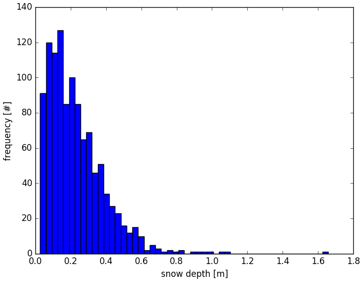
Figure 1 Snow depth data from March and April 2009 to 2013 derived from the OIB data in the RRDP dataset (N=1114) used as input to the scattering model. Mean snow depth is 0.23 m, and the standard deviation is 0.16 m. The minimum snow depth is 0.027 m.

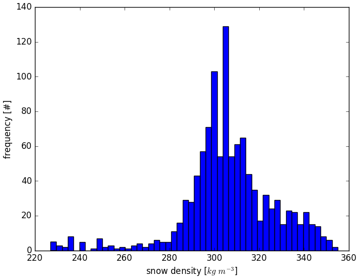
Figure 2 Snow density distribution (N=1114) in the RRDP dataset (from W99 climatology) used as input to the scattering model. Mean snow density corresponding to March and April is 306 kg m⁻³, and the standard deviation is 20 kg m⁻³.

Figure 3 The locations for the RRDP snow depth (Fig. 1) and snow density (Fig. 2) pairs.

Snow geophysical property data

Vertical heterogeneity of snow properties can play a significant role in accurately determining the location of Ka- and Ku-band radar height (Ricker et al., 2014). Since the RRDP lacks information on this vertical heterogeneity, we performed additional simulations using snow geophysical property profiles measured in situ (snow salinity, temperature, and density measurements sampled at 0.02 m vertical intervals) acquired from five disparate snow covers acquired from the Canadian Arctic that ranged in mean thickness from 0.05 to 0.31 cm. These profiles were sampled from land-fast FYI in May 2012 (late-winter season) located near Resolute Bay, Nunavut (74.70^∘ N, 95.63^∘ W). The in situ drill-hole-measured ice thicknesses varied between 1.3 and 1.7 m. We do not have coincident microscale surface roughness estimates measured in situ from these locations, but RADARSAT-2 imagery acquired from this location suggests that each of the five samples was acquired from level and smooth FYI. Here, we assume level sea ice and snow cover with a flat-patch area of 1 % and as a result surface roughness is assumed to not influence the scattering horizon variability in our model simulations. The concept of the flat-patch area is described in the section describing the radar altimeter scattering model below.

Snow temperature was measured in situ using a Digi-Sense RTD thermometer probe (resolution of 0.1 ^∘C and accuracy ±0.2 ^∘C). Snow density was sampled using a 66.35 cm³ density cutter and weighed on a Gram Precision GX-230 scale (accuracy of ±0.01 g). Snow salinity was measured in melted temperature-stabilized samples using a WTW Cond 330i conductivity meter (accuracy of ±0.5 %). The samples were extracted from the snowpack with the density cutter to ensure a comparable sample volume in every sample. Snow grain radius was measured and categorized from disaggregated grain photographs on a 2 mm grid crystal plate following Langlois et al. (2010). The snow grain size and density is used to compute the snow correlation length in Eq. (3) below. The five profiles for which the temperature, snow salinity, and the correlation length are shown in Fig. 4 are as follows.

• Profile 1. The profile comprises 0.05 m cold (snow surface temperature $=-\mathrm{12.7}$ ^∘C), highly saline (7.5–14.5 ppt, parts per thousand) snowpack with a relatively uniform density distribution (320–360 kg m⁻³). The correlation length profile indicates depth hoar layers towards the middle of the snowpack.

• Profile 2. The profile comprises 0.11 m cold (snow surface temperature $=-\mathrm{7.4}$ ^∘C) snowpack, saline at the bottom (14.1 ppt), and nearly non-saline at the top (0.1 ppt). Snow densities in the upper layers are 350 and 250 kg m⁻³ towards the basal layers. The basal layer snow densities and correlation lengths indicate the presence of depth hoar.

• Profile 3. The profile comprises 0.15 m cold (snow surface temperature −12.7 ^∘C) and saline (top to bottom 3–13.3 ppt) snowpack. The top 0.11 m layers have high densities from 400 to 430 kg m⁻³ and the lowest 0.04 m have densities from 220 to 250 kg m⁻³. Similar to Profile 1, the bottom layer densities and the correlation lengths indicate the presence of depth hoar crystals.

• Profile 4. The profile comprises 0.23 m cold (snow surface temperature −13.5 ^∘C), non-saline snowpack. The topmost 0.19 m have low densities (174–267 kg m⁻³), while the bottommost 0.04 m has higher densities (330–350 kg m⁻³). The peaks in correlation length at about 8 cm and at 16 cm are indicating layers of depth hoar.

• Profile 5. The profile comprises 0.31 m almost isothermal (−2.8 to −4.1 ^∘C), highly layered snowpack. Density varies between 226 and 877 kg m⁻³ (icy layers). The bottommost salinity contains up to 5.8 ppt, but the top 0.20 m of the snow profile is non-saline.

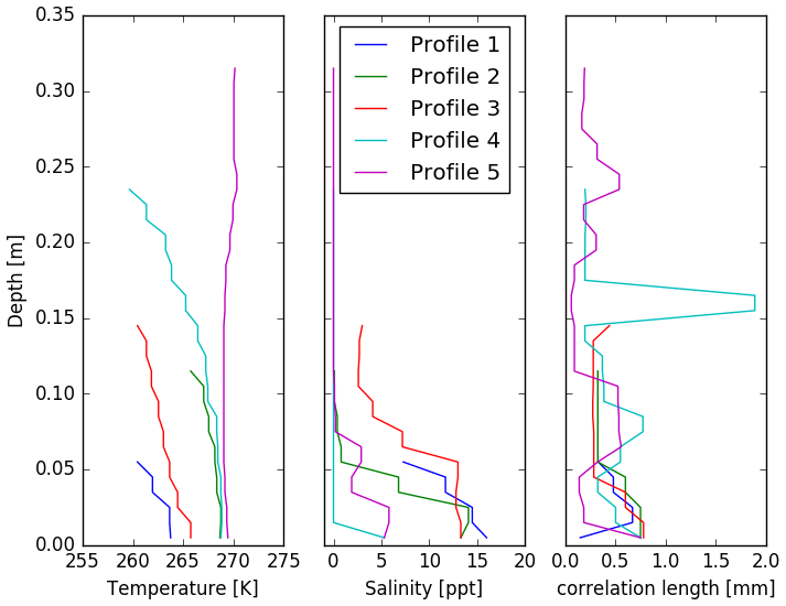
Figure 4 Snow temperature, salinity, and snow grain correlation length of the five snow pit profiles on FYI acquired from the Canadian Arctic. Depth =0.00 corresponds to the bottom of the snowpack.

These five detailed profiles (the snow profiles with 2 m saline FYI beneath) are included in the simulations and are compared to the simulations using a uniform snow profile. Our goal is to separate the direct effect of snow depth in the uniform vertical profile of geophysical properties on the Ka- and Ku-band radar height estimates and compare them with the derived radar height estimations influenced by the effects of layered snowpacks.

3 Radar altimeter scattering model and re-tracker description

The radar scattering model utilized in this study is a multi-layer, one-dimensional radiative transfer model, in which surface scattering is computed at horizontal interfaces (snow surface and interfaces within the snowpack and at the sea ice surface), as described in Tonboe et al. (2006b, 2010) and Tonboe (2017), and it is conceptually comparable to models developed by others (e.g., Landy et al., 2019). The multi-layer model concept is different from single layer scattering models developed for ice sheet backscatter (e.g., Ridley and Partington, 1988) since surface and interface scattering dominates in sea ice (Ulander and Carlström, 1991; Fetterer et al., 1992). The model – flowchart from input of the physical snow and ice profiles to computing the track point – is illustrated in Fig. 5.

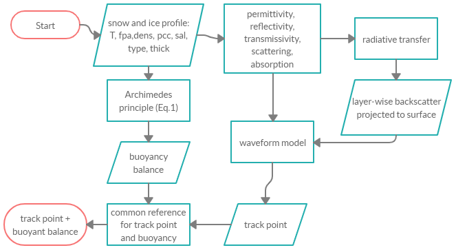
Figure 5 Computational steps in the scattering model to reach the radar altimeter track point. The model is described in detail in Tonboe et al. (2006b, 2010). The snow and ice profile has temperature (T), flat-patch area (fpa), correlation length (pcc), salinity (sal), snow or ice type (type), and thickness (thick) for each layer.

The scattering model uses layer-wise information on snow–sea-ice stratigraphy (layer thickness in meters), temperature (K), snow salinity (ppt), snow density (kg m⁻³), correlation length (a measure of the snow grain size or the size of inclusions, e.g., brine or air in the sea ice) (mm), surface and interface roughness (fraction of total area), and derived brine volume from snow salinity, density, and temperature. The model uses a radiative transfer approach to compute the total backscatter, σ_total (Tonboe et al., 2010).

$$\begin{array}{}\text{(2)}& {\mathit{\sigma }}_{\mathrm{total}}=({\mathit{\sigma }}_i^{\mathrm{surf}}+T_i^{\mathrm{2}}{\mathit{\sigma }}_i^{\mathrm{vol}})\prod _{i=\mathrm{1}}^n{\displaystyle \frac{\mathrm{1}}{L_{i-\mathrm{1}}^{\mathrm{2}}}}{T}_{i-\mathrm{1}}^{\mathrm{2}},\end{array}$$

where ${\mathit{\sigma }}_i^{\mathrm{surf}}$ is the surface and interface scattering for layer i, T_i is the surface and interface transmissivity, ${\mathit{\sigma }}_i^{\mathrm{vol}}$ is the layer volume scattering, and L is the layer loss (scattering and absorption). The volume scattering is a function of radar frequency to the 4th power. It is the parameter which is most sensitive to radar frequency, but all the parameters in Eq. (2) are to some extent frequency dependent. Radar propagation speed, attenuation and scattering are computed for each layer. We use a geometric description of the footprint area in each layer as a function of time for a pulse limited altimeter, and the time-dependent area is multiplied by the time-dependent backscatter resulting in the waveform (Tonboe et al., 2010). The track point is found at half of the maximum waveform power point in time (Tonboe et al., 2010). While different track point thresholds will shift the track point vertically (Ricker et al., 2014), the location of the track point does not change the modeled sensitivity to snow depth (Tonboe, 2017).

Since the total backscatter is dominated by surface and interface scattering, the surface scattering model used in this study assumes that the backscatter return signal is dominated by specular reflection processes from relatively small plane areas (flat-patches), which are normal to the near-nadir radar signal within the footprint, described in Fetterer et al. (1992; Eq. 18) and Ulander and Carlström (1991). This assumption is believed to be “more realistic” than, for example, the assumptions behind the geometric optics model because the satellite nadir or near-nadir radar backscatter is dominated by reflections from smooth patches on the surface (Fetterer et al., 1992). The fundamental assumption for all radar altimeter surface scattering models is that the backscatter is a function of the reflection coefficient, interface roughness, and slope; i.e., when the interface is smooth, the backscatter is high, and when the surface is rough, then the backscatter received by the radar is smaller.

The permittivity of the snow and ice is computed using the two-phase mixing formulas described in Mätzler (1998). The permittivity of dry snow is primarily a function of snow density, and the permittivity of sea ice and saline snow depends on salinity and temperature, i.e., brine volume and snow or ice density (Frankenstein and Garner, 1967; Drinkwater and Crocker, 1988). The permittivity of both materials is computed using the mixing formulae for rounded spheres as inclusions in a background matrix of air or ice (Mätzler, 1998) and the equations for brine volume and permittivity in Ulaby et al. (1986). When the snow is saline, we use a formulation for wet snow in Ulaby et al. (1986) and an estimation of the brine volume as a function of salinity, density, and temperature (Ulaby et al., 1986). This is feasible since the permittivity of fresh water and brine is the same for radar frequencies larger than about 10 GHz, including both Ka- and Ku-bands (Ulaby et al., 1986). The predictions of different snow and ice permittivity models vary as a function of brine pocket, air bubble, or snow particle inclusion shape and permittivity (Ulaby et al., 1986). We believe that the choice of model will have an impact on the absolute magnitude of the model estimates, however, only a smaller impact on the relative variability of the model predictions. Volume scattering from snow grains or inclusions in the ice is computed for each layer using the “improved Born approximation” for spherical inclusions (Mätzler, 1998) and is included in our radiative transfer calculation. Although the volume scattering contribution to the overall backscatter is considered insignificant, its contribution adds to the signal extinction and therefore affects the loss factor and the track point.

We convert the optical snow grain size (described in the detailed snow profiles) to snow correlation length, pcc, which is used in the model describing the scatter size, i.e., (Mätzler, 2002),

$$\begin{array}{}\text{(3)}& \text{pcc}=\mathrm{0.5}{D}_{\mathrm{0}}(\mathrm{1}-v),\end{array}$$

where D₀ is the optical snow grain diameter in millimeters and v is the bulk snow density divided by the pure ice density (917 kg m⁻³).

In this study, the track point is computed as a point in time located midway between zero backscatter and the maximum return signal power received by the radar. Different track point thresholds change the vertical height of the scattering horizon, as described in Tonboe (2017). On ice sheets and sea ice where surface and interface scattering dominates, the half power time re-tracking threshold provides a good estimate of the mean surface elevation (Davis, 1997).

4 Scattering model initialization and setup

The scattering model uses a multi-layer snow and sea ice profile as input. The simplest case consists of one uniform snow layer on top of an overlying uniform ice layer, with the parameters listed in Table 1 used as input to the model. While salinity, temperature, and interface roughness are fixed, snow depth and density vary, as given in the RRDP dataset. We set pcc to 0.1 mm following Tonboe et al. (2010) and Tonboe (2017). For snow and ice salinity and temperature, we assume a brine-free snowpack and an isothermal temperature of 263.15 K. Sea ice salinity and temperature are set at 3.0 ppt and 269.15 K, respectively. These values represent non-melting conditions. Here, the flat-patch area is set to 0.01 for both the snow and the sea ice surface (Tonboe et al., 2010). With this information, the model produces the backscatter coefficient, waveform, and track points at half of the maximum power. The model then simulates the Ka- and Ku-band radar waveform track point variability in homogeneous snowpacks during winter as a function of snow depth and density only. Since both the track point and the floe buoyancy are affected by snow depth and density, the scattering model is used, together with the Archimedes principle, to compute the sensitivity of both simultaneously. The fixed value of surface roughness used in these simulations at the snow surface and at the snow–ice interface will affect the height of the scattering surface for both Ka- and Ku bands, while the sea ice density will primarily affect the floe buoyancy's impact on the track point (Tonboe et al., 2010).

The scattering model is first initiated with uniform snow and sea ice properties and then for each subsequent simulation, the snow density and snow depth in Table 1 are exchanged with OIB pairs of snow depth and the Warren et al. (1999) snow density from the RRDP dataset in order to investigate the sensitivity to observed snow depth and density variability. Then we additionally use the five snow geophysical property profiles to study the effect of snow density layering and variability in snow salinity and grain size on the track point.

Table 1 Initial run input to the scattering model. T is the layer temperature, roughness is quantified as the flat-patch area which is the fraction of specular facets compared to the total area (F), density is the layer density, depth is the layer thickness, correlation length is a measure of the scatter size (and distribution), and salinity is layer salinity. Variables marked in bold in the table are exchanged with values from the RRDP for each simulation. There are 1114 data points in the RRDP dataset.

5 Ka- and Ku-band altimetry track point difference simulation results and discussion

The Ka- and Ku-band track point difference as a function of snow depth, density, and correlation length is illustrated in Fig. 6. We find that the Ka- and Ku-band track point difference ranges between 0 and 0.08 m for coarse-grained (pcc =0.3 mm) snow depths between 0.05 and 0.65 m. The sensitivity increases with snow depth and is highest for snow deeper than 0.5 m. The sensitivity to snow depth decreases for smaller snow correlation lengths such that the track point difference is about half (0 to 0.04 m) for fine-grained snow (correlation length of 0.1 mm shown in red) compared to coarse-grained snow (correlation length of 0.3 mm shown in blue), keeping all other parameters unchanged (see Table 1). We are not varying the surface roughness in our experiments. To investigate the impact of the air–snow and snow–ice interface roughnesses on the Ka- and Ku-band track point difference, we would require a different surface scattering model and data to account for the interface roughness. This remains outside the scope of this study.

Figure 6 illustrates the effect of the five snow profiles on FYI in the Canadian Arctic. Of interest is the presence of saline snow covers on FYI, which has been long recognized for its effect on radar signal propagation (Geldsetzer et al., 2007; Yackel and Barber, 2007; Nandan et al., 2020, 2017b; Kwok and Kacimi, 2018; Barber and Nghiem, 1999; Barber et al., 1998, and references therein). With changes in snow temperature, salinity, and density in the snow layers, snow brine volume is modified towards the snow basal layers and at the snow–sea-ice interface, masking the propagation of radar waves from reaching the snow–sea-ice interface (Barber and Nghiem, 1999; Nandan et al., 2017a). This results in an upward shift of the track point. In our study, the simulations were rerun at 1 % snow brine volume (1 % brine volume is equivalent to a bulk snow salinity of about 2 ppt at −10 ^∘C bulk snow temperature), after which the Ka- and Ku-band track point differences were acquired. For snow covers <0.1 m, the saline snow at first increases the sensitivity of the Ka- and Ku-band track point difference to snow depth, but for snow depths >0.1 m, the signal loss in the snow cover caused by the brine results in identical track points at the Ka- and Ku-band. Snow extinction is the sum of scattering from snow grains and attenuation from brine when the snow is saline. While attenuation in the snow is comparable at the Ka- and Ku-band, scattering is different, and it is the scattering contribution to the extinction which is creating the Ka- and Ku-band track point difference. Deeper snow (more scatters) and/or larger snow grains (scatters) gives more scattering and a larger Ka- and Ku-band difference by increasing extinction and the relative importance of the snow–ice interface scattering. When the depth of saline snow is increased, then the Ka- and Ku-band track point difference initially increases compared to non-saline snow. This is because the attenuation is controlling the relative importance of the snow–ice interface scattering compared to the snow surface scattering which is invariant in these experiments, and again it is the scattering from the snow grains which is producing the Ka- and Ku-band track point difference. When the snow depth is >0.1 m, then the relative importance of the snow–ice interface scattering is minimal. When the saline snow is ∼0.4 m thick, then snow surface scattering totally dominates, and there is no Ka- and Ku-band track point difference because both radar wavelengths are scattered at the snow surface. The average sensitivity of the Ka- and Ku-band track point difference to snow depth in our simulations is small (30:1). For coarse-grained snow, using the mean snow depth from the RRDP dataset of 0.23 m as the reference point, the track point difference is 0.008 m (Fig. 4). This indicates that the Ka- and Ku-band track point differences observed in Lawrence et al. (2018) and in Guerreiro et al. (2016) are not only caused by the snow depth itself but in combination with, for example, the snow grain size and/or snow salinity or other factors that we have not investigated here. Armitage and Ridout (2015) found that the Ka- and Ku-band track point difference is a function of sea ice type as well. Snow depth is indirectly linked with sea ice type because the accumulation period is longer, generating thicker and denser snow for second-year ice (SYI) and MYI and also because SYI and MYI are rougher and disproportionately “trap/capture/entrain” more drifting snow than for FYI (Iacozza and Barber, 1999; Liston et al., 2019). In addition, snow cover on FYI is usually saline, especially in the 0.06 to 0.08 m basal layers (Drinkwater and Crocker, 1988; Barber et al., 1998; Nandan et al., 2017b), and this will affect the Ka- and Ku-band track point difference.

Sensitivity of the Ka- and Ku-band track point difference to variations in snowpack properties from our five profiles is summarized in Table 2. The track point difference is essentially zero when the snow is saline. However, profile 4 (non-saline snowpack with depth of 0.23 m) has a Ka- and Ku-band track point difference of 0.05–0.08 m, which is comparable to differences reported by Armitage and Ridout (2015). This illustrates that the track point difference can be higher for naturally observed snow profiles than for the uniform profile results shown in Fig. 6. In addition to being non-saline, profile 4 has layers with coarse-grained snow. The snow correlation length in these layers is much larger than for any of the other profiles. The scattering magnitude contributing to the radar signal extinction in the snow at the Ka- and Ku-bands is very different, and this is affecting radar penetration and consequently the track point difference in profile 4.

Table 2 Summary of the Ka- and Ku-band track point difference for five snow profiles on FYI in the Canadian Arctic.

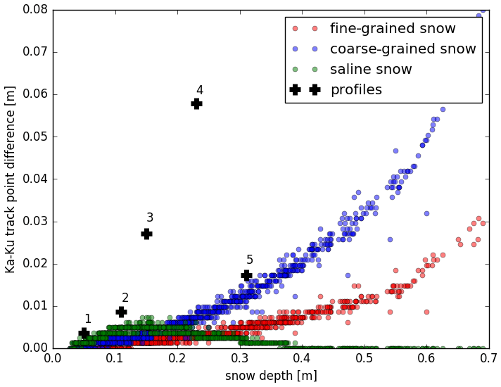
Figure 6 The Ka- and Ku-band track point difference as a function of snow depth (and density). The red points represent the profile in Table 1, while blue points represent coarse-grained snow (correlation length: 0.3 mm), and green points represent saline snow (salinity 2 ppt). The five simulated profiles in Table 2 are marked with black crosses, and the numbers refer to the profile number in Table 2.

6 Snow climatology for radar sea ice freeboard to thickness conversion

It is common practice in sea ice altimetry to use the W99 snow climatology in the F_I to H_I conversion (Laxon et al., 2013; Kurtz and Farrell, 2011). The snow climatology is used to (1) compensate for the effect of the snow cover on the ice floe buoyancy and (2) compute radar pulse propagation speed reduction in the snow which is affecting the range estimation. In practice, on a location-specific basis, the snow climatology only introduces a systematic uncertainty in the sea ice thickness estimation since the climatology does not reflect actual spatial and temporal snow depth and density variability. Here, we simulate the radar track point as a function of snow depth to see the combined effect of (1) and (2).

Figure 7 summarizes the simulated Ka- and Ku-band radar track points computed with the scattering model and the snow–sea-ice interface computed from the buoyancy of the profile as a function of the snow depth and density using (1) the uniform profile (Table 1) with varying snow depth and density from the RRDP data and (2) the snow profiles from the Canadian Arctic. We do not show the actual ice thickness, which is 2 m in our simulations, only the Ka- and Ku-band track points and the snow–ice interface. The water surface height is estimated with the model and the re-tracker. Both the snow depth and the snow density are varied in the simulations. However, the effect of snow density is negligible because its variability in the RRDP dataset is small (mean snow density is 306 kg m⁻³ and the standard deviation is 20 kg m⁻³; see Fig. 2). Moreover, the standard deviation of the snow density in the RRDP dataset is small compared to other studies (e.g., King et al., 2020). Linear fits to each of the clusters are shown. The snow profiles from the Canadian Arctic, exhibiting larger vertical variability in snow density, are in close agreement with the fitted simulations for the reference snow profile. In Fig. 7, the snow–ice interface height is decreasing as a function of increasing snow depth ($f=-\mathrm{0.29}\text{SnowDepth}+\mathrm{0.24}$), while the Ku-band track point height is increasing as a function of increasing snow depth ($f_{\mathrm{Ku}}=\mathrm{0.35}\text{SnowDepth}+\mathrm{0.24}$). The Ka-band track point is also increasing as a function of increasing snow depth ($f_{\mathrm{Ka}}=\mathrm{0.39}\text{SnowDepth}+\mathrm{0.24}$).

The green line in Fig. 7 shows the combined effect of snow on the Ku-band track point and the floe buoyancy. The slope is small ($f=\mathrm{0.03}\text{SnowDepth}+\mathrm{0.34}$), suggesting that the combined effect of the radar track point and the floe buoyancy variability is almost independent of snow depth. The combined effect of the Ka-band track point and the floe buoyancy is $f_{\mathrm{Ka}}=\mathrm{0.05}\text{SnowDepth}+\mathrm{0.15}$.

The effect of snow depth on the Ku- and Ka- track point is linear up to snow depths of ∼0.5 m (Fig. 7). Therefore, even if the RRDP data are not fully representative of the Arctic, the results would still be valid for most of the Arctic because snow depth on Arctic sea ice is usually <0.5 m. The radar pulse propagation speed reduction correction for the Ku-band track point in our simulations is on average 0.35 times the snow depth (slope of red line in Fig. 7) for a snow density of 306 kg m⁻³ (standard deviation 20 kg m⁻³). This is comparable to the correction used in CryoSat-2 operational processing (Tilling et al., 2018),

$$\begin{array}{}\text{(4)}& \mathit{\delta }h=\mathrm{0.25}\text{SnowDepth},\end{array}$$

so that the freeboard correction δhs is 25 % of the snow depth. This equation is valid for a snow density of 300 kg m⁻³. The buoyancy correction in our simulations is on average 0.29 times (slope of the blue line in Fig. 7) the snow depth with an opposite sign (+/−) to the track point correction. This is equivalent to the buoyancy correction described in Eq. (1) for both FYI and SYI for a snow density of 300 kg m⁻³. The snow geophysical property profiles from the Canadian Arctic, with a range of snow depths (0.05–0.31 m), show a similar pattern as the uniform profiles for both the floe buoyancy and track point (Fig. 7).

Therefore, the correction for snow on buoyancy and Ka- and Ku-band track point are almost equal and opposite in magnitude. This means that if actual snow depth information is available, then the radar freeboard should be corrected for both the track point and buoyancy variation before computing sea ice thickness on a location-specific basis.

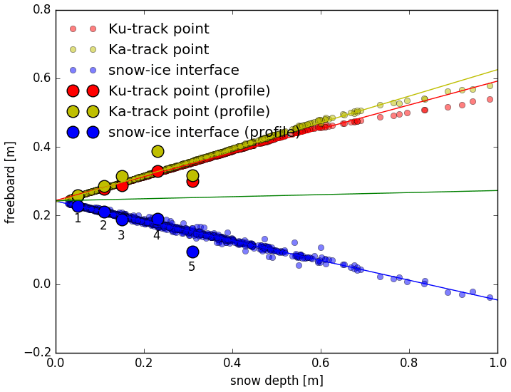
Figure 7 Red circles are the Ku-band radar track point as a function of snow depth and density, the linear fit (red line) is the freeboard, $f_{\mathrm{Ku}}=\mathrm{0.35}\text{SnowDepth}+\mathrm{0.24}$, yellow circles (and line) are the Ka-track point, $f_{\mathrm{Ka}}=\mathrm{0.39}\text{SnowDepth}+\mathrm{0.24}$, blue circles are the snow–ice interface freeboard as a function of snow depth and density, and the linear fit (blue line) is $f=-\mathrm{0.29}\text{SnowDepth}+\mathrm{0.24}$. The combined effect of the Ku-band track point and buoyancy is the green line freeboard, $f=\mathrm{0.03}\text{SnowDepth}+\mathrm{0.34}$. The five snow profiles (numbers 1–5) from the Canadian Arctic are added and are depicted with large blue circles for the snow–sea-ice interface and large red and yellow circles for the Ka- and Ku-band track points, respectively (Table 2). (The figure is a reproduction of Fig. 3c in Tonboe et al., 2010, with new input data).

The W99 snow climatology used to convert F_I to H_I is seasonally and regionally varying. This means that the systematic uncertainty that the W99 dataset introduces in the sea ice thickness derivation has regional and seasonal variability. However, this variability may not coincide with actual snow depth and density. With increasingly earlier Arctic sea ice melt onset and longer melt seasons (e.g., Stroeve and Notz, 2018), sea ice freeze onset and snow accumulation time has also reduced (Webster et al., 2014, 2018). Deviations in snow depth and density from climatology are mapped directly as systematic errors into the derived sea ice thickness changes. Climatology is used when the real snow depth is unknown, and the offset that the climatological snow depth is introducing to the Ku-band freeboard measurement is 0.03 times the climatological snow depth (the green-line slope in Fig. 7). Additionally, there is a 0.03 times the real snow depth bias when using snow climatology. If not using the climatology, there would only be the 0.03 times the real snow depth bias, and only if the real snow depth is known can the bias be avoided. This has two important implications: (1) the snow climatology results in a small impact on the derived sea ice thickness because the radar penetration and the buoyancy correction have opposite signs (−/+), and (2) when using climatology, a bias is introduced by the freeboard sensitivity to snow coming from the climatology and the actual snow cover variability. The small impact of the snow on the measured freeboard is the reason why the sea ice thickness can be derived using radar altimeters even without actual snow information (current operational situation). It is also the reason why corrections using snow climatology are relatively small compared to other errors. Other factors related to snow could influence the buoyancy and the radar scattering, e.g., snow salinity and density (e.g., Nandan et al., 2017a, 2020), snow grain size, roughness (e.g., Tonboe et al., 2010; Landy et al., 2020), and snow layering; these topics warrant further research.

7 Conclusions

In this study, we have shown that it is necessary to correct the sea ice freeboard measured by a radar altimeter for both the snow loading from actual snow depth estimates and the radar signal penetration before computing the sea ice thickness. As a result, we advocate avoiding the use of snow climatology because we think it is not necessary to include a bias in sea ice thickness estimation even if it is small. We used a radar scattering model forced with snow depth and density from the European Space Agency's RRDP dataset and snow geophysical property profiles measured in situ obtained from land fast FYI in the Canadian Arctic.

Our simulations indicate that the direct Ka- and Ku-band track point difference sensitivity is about 0.033 times the snow depth using the average snow depth of 0.23 m as a reference point. This is smaller than previously reported from SARAL/AltiKa Ka-band and CryoSat-2 Ku-band track point differences of ∼0.04 to 0.07 m from October to March over the AltiKa region of coverage (e.g., Armitage and Ridout, 2015; Guerreiro et al., 2016; Lawrence et al., 2018). The simulated Ka- and Ku-band track point sensitivity is affected by snow grain size, snow salinity, and vertical snow density heterogeneity, in addition to the snow depth itself. However, the simulated Ka- and Ku-band track point differences do not explain all of the observed differences, and other factors, such as ice type (with corresponding snow salinity and snow grain size), likely affect the differences as well (Armitage and Ridout, 2015). Saline snow on FYI dampens the Ka- and Ku-band track point difference by masking the penetration of both Ka- and Ku-band radar waves from reaching the snow–sea-ice interface. This result was found using both the uniform and detailed snow geophysical property profiles as input to the model and supports the findings of Armitage and Ridout (2015) who noted that the Ka- and Ku-band track point difference is dependent on sea ice type. Snow scattering creates a Ka- and Ku-band track point difference by controlling the relative importance of the snow–ice interface scattering compared to snow surface scattering. This was shown for both the uniform profiles and the detailed snow geophysical property profiles.

The buoyancy and Ka- and Ku-band track point corrections are nearly equal and opposite in magnitude. This implies that the measured freeboard is nearly independent of snow depth. The measured Ku-band freeboard is elevated (lowered) by about 0.03 times the snow depth with an increase (decrease) in snow depth. For the Ka-band, the factor is 0.05. This has two implications when deriving the sea ice thickness from the radar freeboard: (1) the snow depth climatology introduces a bias in the measured Ku-band freeboard of 0.03 times the climatological snow depth plus 0.03 times the real snow depth, and (2) the impact of actual snow depth is small in the sea ice thickness estimate and if the actual snow depth is unknown, it is better not to correct than to use climatology for the correction.

A high-inclination polar-orbiting Ka- and Ku-band radar altimeter (CRISTAL) is being planned at ESA as one of six European Copernicus High Priority Candidate Missions for launch after 2026 (Kern et al., 2020). A primary objective of CRISTAL is to improve upon the accuracy of snow and sea ice thickness estimates. We anticipate that our simulations will be useful in consolidating these applications and improve the measurement and mapping of snow and ice thickness from space.