the Creative Commons Attribution 4.0 License.
the Creative Commons Attribution 4.0 License.
 | 24 Mar 2021
Snow depth mapping with unpiloted aerial system lidar observations: a case study in Durham, New Hampshire, United States
Jennifer M. Jacobs
Adam G. Hunsaker
Franklin B. Sullivan
Michael Palace
Elizabeth A. Burakowski
Christina Herrick
Eunsang Cho
Terrestrial and airborne laser scanning and structure from motion techniques have emerged as viable methods to map snow depths. While these systems have advanced snow hydrology, these techniques have noted limitations in either horizontal or vertical resolution. Lidar on an unpiloted aerial vehicle (UAV) is another potential method to observe field- and slope-scale variations at the vertical resolutions needed to resolve local variations in snowpack depth and to quantify snow depth when snowpacks are shallow. This paper provides some of the earliest snow depth mapping results on the landscape scale that were measured using lidar on a UAV. The system, which uses modest-cost, commercially available components, was assessed in a mixed deciduous and coniferous forest and open field for a thin snowpack (< 20 cm). The lidar-classified point clouds had an average of 90 and 364 points/m2 ground returns in the forest and field, respectively. In the field, in situ and lidar mean snow depths, at 0.4 m horizontal resolution, had a mean absolute difference of 0.96 cm and a root mean square error of 1.22 cm. At 1 m horizontal resolution, the field snow depth confidence intervals were consistently less than 1 cm. The forest areas had reduced performance with a mean absolute difference of 9.6 cm, a root mean square error of 10.5 cm, and an average one-sided confidence interval of 3.5 cm. Although the mean lidar snow depths were only 10.3 cm in the field and 6.0 cm in the forest, a pairwise Steel–Dwass test showed that snow depths were significantly different between the coniferous forest, the deciduous forest, and the field land covers (p < 0.0001). Snow depths were shallower, and snow depth confidence intervals were higher in areas with steep slopes. Results of this study suggest that performance depends on both the point cloud density, which can be increased or decreased by modifying the flight plan over different vegetation types, and the grid cell variability that depends on site surface conditions.
- Article
(8267 KB) - Full-text XML
-
Supplement
(2199 KB) - BibTeX
- EndNote


Over the past 2 decades, remote-sensing methods, providing spatially continuous, high-resolution snow depth maps at local and regional scales, have greatly advanced the ability to characterize the spatiotemporal variability in snow depth over earlier work using snow probes. Spaceborne photogrammetry (e.g., Marti et al., 2016; McGrath et al., 2019; Shaw et al., 2020), airborne laser scanning (ALS) (Deems et al., 2013; Harpold et al., 2014; Kirchner et al., 2014), terrestrial laser scanning (TLS) (Grünewald et al., 2010; Currier et al., 2019), and structure-from-motion photogrammetry (SfM) (Nolan et al., 2015; Bühler et al., 2016; Harder et al., 2016) have emerged as viable methods to map surface elevations with snow-off and snow-on conditions in order to differentially map snow depths.
ALS and TLS both rely on well-established lidar (light detection and ranging) technology. TLS, applied from a fixed ground position, is able to measure snow depth with high vertical accuracy (Fey et al., 2019) and has the advantage of being relatively low-cost and portable, making repeat observations possible. However, TLS uncertainties are caused by large incident angles, occlusion from hills and trees that can cause data gaps in forested domains (Currier et al., 2019; Palace et al., 2016), and challenges to provide a stable scanner position for the tripod in snow-on conditions (Schweizer et al., 2003). ALS technology such as that deployed on the Airborne Snow Observatory (ASO) (Painter et al., 2016) has the advantage of being able to cover large areas, but it is extremely expensive and has limited availability and flexibility of deployment, which impacts its use for most studies. ALS also has issues with observation gaps in forested regions (Broxton et al., 2015; Currier and Lundquist, 2018; Mazzotti et al., 2019) but possibly to a lesser extent than TLS (Currier et al., 2019). The typical vertical accuracies from these platforms are on the order of 10 cm (Kraus and Pfeirer, 2011; Deems et al., 2013) with a relatively low return density (∼ 10 returns/m2) (Cook et al., 2013). These accuracies and densities may not be adequate to observe spatial variations at point scales (0 to 5 m) to hillslope and field scales (1–100 m) and to detect snow depth changes over short timescales due to single events, densification, wind redistribution, sloughing of snow-off slopes, trapping of snow by vegetation, and forest canopy interception (Clark et al., 2011; Mott et al., 2011, 2018).
SfM can create a digital surface model (DSM) from photographs taken using a standard consumer-grade digital camera. When using an unpiloted aerial system (UAS), which deploys a camera on an unpiloted aerial vehicle (UAV), SfM is a low-cost method that has the capacity for routine snow depth monitoring (Adams et al., 2018; Bühler et al., 2016; De Michele et al., 2016; Harder et al., 2016; Vander Jagt et al., 2015). Reported accuracies range from 8 to 30 cm using UAS SfM (Adams et al., 2018; Bühler et al., 2016; Goetz and Brenning, 2019; Harder et al., 2016; Meyer and Skiles, 2019; Harder et al., 2020). The primary drawbacks of UAS SfM as compared to lidar for mapping snow depth are that the DSM needs to be georeferenced using ground control points (GCPs) with known coordinates and may require significant manual steps (Tonkin and Midgley, 2016; Meyer and Skiles, 2019), although new techniques are emerging that may reduce field data collection time (Gabrlik et al., 2019; Meyer and Skiles, 2019). Dense canopy or vegetation can reduce performance when snow compresses the vegetation relative to the snow-off imagery or when above-canopy vegetation is falsely interpreted to be the snow surface (Bühler et al., 2017; Cimoli et al., 2017; De Michele et al., 2016; Fernandes et al., 2018; Harder et al., 2016; Nolan et al., 2015). Canopy effects impact SfM snow mapping capability in regions where snowpacks are masked by dense forest canopies. The inability to sense portions of the ground or snow surface beneath dense canopies results in fine-scale variations in snow depth, such as tree wells, not being accurately represented in UAS SfM snow depth products (Harder et al., 2020).
UAS lidar, a UAV-mounted laser scanning system, has been widely used in forest-related research (e.g., canopy height and forest change detection) (Wallace et al., 2012, 2014) and appears to offer the advantages of both the UAS SfM and lidar for snow depth mapping. UAS lidar also eliminates many of the drawbacks that arise from ALS and TLS systems discussed earlier. However, to date there is only one previous study that estimates snow depth using UAS-based lidar (Harder et al., 2020). Harder et al. (2020) compared snow depth estimates between lidar versus SfM techniques using in situ snow depth observations in mountain and prairie environments, focusing on sub-canopy snow, which has been a challenge to measure in the snow remote-sensing community. Using a considerably more expensive UAS-based lidar system (∼ CAD 300K), they found that the lidar system tends to have lower errors than the SfM to capture sub-canopy snow distributions at moderate depth of snowpack (up to 2 and 1 m of the maximum depth for mountain and prairie areas, respectively). In this study, we assess the ability of a more modest-cost UAS lidar system (∼ USD 70K) to map snow depth, focusing on shallow and ephemeral snowpack (< 20 cm). The pilot study described here serves as a proof of concept for providing a high-vertical-resolution snowpack data set in open terrain and forests in the northeastern United States. Snow depth magnitude and variability are mapped and analyzed for differences by land use and slope. The study highlights results from the 2019 winter season that provide insights as to the potential for UAS lidar mapping of snow depth as well as details about the system, its deployment, and operational and validation challenges. We explore the capability of UAS through the comparison of contemporary field-based snow depth measurements collected in a landscape containing fields and forests.
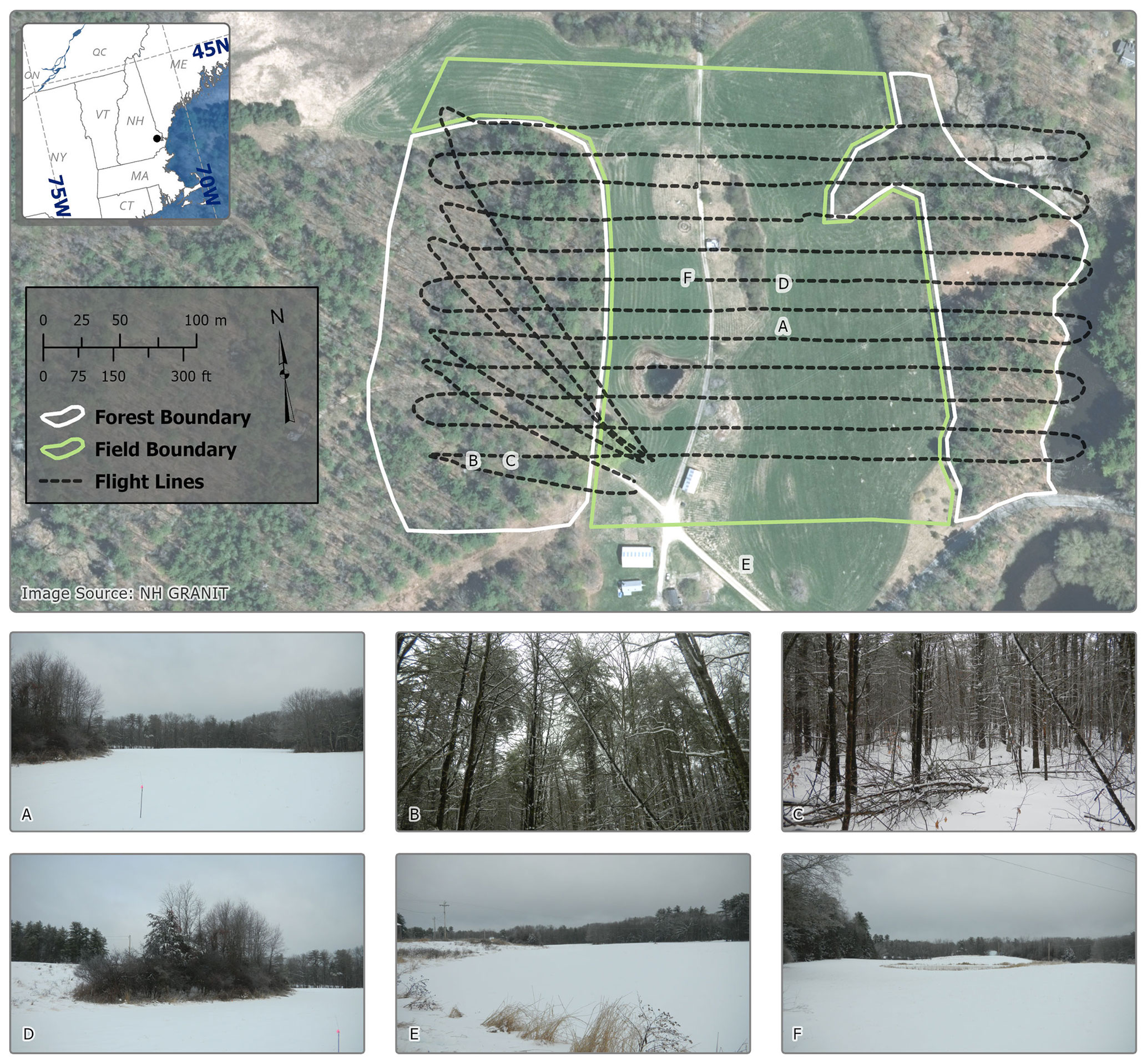
Figure 1Aerial imagery of Thompson Farm, Durham, NH, from 2015 showing both forest and field regions with lidar flight lines (top). Ground imagery (A to F) collected in December 2019; locations are noted on the top map and show the surface and leaf-off forest conditions (bottom panels).
2.1 Site
The test flights were conducted at the University of New Hampshire's Thompson Farm Research Observatory in southeastern New Hampshire, United States (43.10892∘ N, 70.94853∘ W; 35 m above sea level, a.s.l.), which was chosen for its mixed-hardwood-forest and open-field land covers (Burakowski et al., 2015; Burakowski et al., 2018) that are characteristic of the region (Fig. 1). Thompson Farm has an area of 0.83 km2 and little topographic relief (Perron et al., 2004). The agricultural fields are actively managed for pasture grass. The mixed deciduous and coniferous forest is composed primarily of white pine (Pinus strobus), northern red oak (Quercus rubra), red maple (Acer rubrum), shagbark hickory (Carya ovata), and white oak (Quercus alba) (Perron et al., 2004). There are two logging access roads that run north–south through the pasture and into the western forest section.
2.2 UAS laser scanning
A series of UAS lidar surveys were conducted over approximately a 0.1 km2 (9.8 ha) area (430 m × 225 m) within the farm during the winter 2018/2019 (Fig. 1). Here, we focus on the snow-on flight conducted on 23 January 2019 and the snow-off flight conducted on 11 April 2019. We selected the 23 January 2019 flight because it had snowed approximately 11.5 cm, with 1.8 cm of snow water equivalent from 19 to 20 January 2019, and the air temperature was persistently below freezing prior to the flight. For the 11 April 2019 snow-off flight, the deciduous component of the canopy and understory was both dormant.
We used an Eagle XF UAS manufactured by UAV America, which carried a small, lightweight lidar sensor (Velodyne VLP-16) suitable for UAS deployment (see Table S1 in the Supplement). The VLP-16 is a 16-channel lidar sensor with a 30∘ vertical field of view with rotating lasers that are spaced evenly between −15 and +15∘. Each channel rotates to provide a horizontal field of view of 360∘. The VLP-16 collects up to 300 000 points per second with an accuracy of ±3 cm at a range of 100 m. The sensor was mounted with the vertical field of view parallel with the ground. The payload is equipped with an Applanix APX-15 UAV inertial navigation system (INS), which has 2–5 cm positional, 0.025∘ roll and pitch, and 0.08∘ true heading uncertainties following post-processing. The INS has a measurement rate of 200 Hz, allowing for a timestamp to associate each lidar pulse with the closest data for latitude, longitude, altitude, and perspective information (roll, pitch, and yaw), which is required for georeferencing returns.
Flights were conducted to maximize spatial coverage while conserving batteries due to the limited flight time of the Eagle XF (approx. 9 min flight time from ascent to descent). Because of the limited flight time, flights were conducted at an altitude of 81 m for greater spatial coverage, and multiple return flight lines were necessary for battery exchanges (Fig. 1). Automated flights were conducted using UgCS flight planning software. Flight speed was 7 m/s, with a total of 12 parallel flight lines with targeted overlap of 40 %. A complete survey of the study area took approximately 2 h. This includes the time required to calibrate the INS and set up and break down the UAS. Because of degrading accuracy at distances > 100 m with the VLP-16, returns acquired outside of ±30∘ of nadir view angles in the horizontal field of view were filtered to limit target distance and improve overall accuracy.
Applanix APX-15 INS data were post-processed to a Smoothed Best Estimate of Trajectory (SBET) file using POSPac Mobile Mapping Suite (MMS) UAV (v. 8.2.1), resulting in approximately 3 cm positional accuracy for both the snow-on and snow-off flights. Lidar returns were individually georeferenced by synching timestamps of returns from the lidar sensor with timestamps of position and attitude data from the post-processed INS data. Georeferenced point clouds were produced and output to LAS (LASer) files using Headwall Photonics, Inc.'s LidarTools software. The bare-earth and snow-on point clouds were georeferenced solely using the INS data respective to each flight. The point clouds were not co-registered to each other as there were no reliable common ground control points between surveys. For UAS lidar snow depth surveying, co-registration between point clouds would likely be unattainable due to insufficient common ground control. We determined that results would be more meaningful when bare-earth and snow-on point clouds were processed solely relying on the capability of the INS. Boresighting calibration was performed using returns from the first two parallel flight lines that were collected in opposite directions (i.e., antiparallel). A roll offset was determined using 10 m cross-sections along the flight lines over flat terrain, and a pitch offset was determined using 1 m cross-sections across the flight lines over terrain with moderate relief (see Fig. S2 in the Supplement). Resulting LAS point clouds were generated for the entire study area and projected in WGS84 UTM Zone 19N (EPSG 32619). Flight and filtering parameters of the raw point cloud resulted in return densities of approximately 150 returns/m2 for each of the two flights.
2.3 Lidar classification and gridding
Three-dimensional point clouds were processed using the progressive morphological filter algorithm (PMF) in the lidR package (https://github.com/Jean-Romain/lidR, last access: 3 March 2021) of R (v. 3.4; R Core Team, 2020) to identify ground returns. Briefly, the PMF operates iteratively on sets of two parameters, window size and elevation thresholds, to erode and dilate point cloud data sets to estimate surface topography. The result of the PMF is that non-ground returns (i.e., trees, shrubs, and noise) are filtered out of point cloud data sets so that only returns from ground surfaces remain. The two data sets, non-ground returns and ground returns from the original point cloud, are coded according to LAS specifications and merged. For a full explanation of the PMF, see Zhang et al. (2003). For ground classification, point clouds were chunked into 100 m square tiles with a 15 m buffer on all sides using catalog options in lidR to ensure returns near tile edges were classified. Processing was distributed across eight computing cores to improve efficiency. The PMF was parameterized using a set of window sizes of 1, 3, 5, and 9 m and elevation thresholds of 0.2, 1.5, 3, and 7 m, which were determined by varying value sets and assessing digital terrain models (DTMs) to determine the parameter sets that produced a visually smooth surface over a dense grid (sensu Muir et al., 2017). Following ground classification for each tile, returns within the 15 m tile buffers were removed, and all resulting 100 m square ground-classified tiles were merged. The resulting point clouds for each data set included both the classified ground returns and the non-ground returns. Snow-on and snow-off ground point clouds were gridded at 0.1, 0.2, 0.4, 0.5, and 1.0 m spatial resolutions using the average of all grid points within each grid cell (Currier et al., 2019). Gridded products for each data set were forced to the same coordinate grid to generate DTMs as raster files.
2.4 Slope and vegetation cover classification and analysis
The snow-off DTM was used to develop a 1 m resolution map of slope (Horn, 1981). Vegetation cover type (field or forest) was determined from optical imagery. A canopy height model (CHM) was developed by subtracting the DTM produced using ground-classified points from the DSM produced using all lidar points. This results in a digital model consisting solely of canopy heights with no topography. The CHM generation used raster images with a 1 m resolution. The forested area was further classified as coniferous or deciduous for the study region. Within the forested area, the CHM was used to distinguish the upper canopy that did not lose needles or foliage from other forested regions with trees with no leaves using our snow-off survey that was collected in leaf-off conditions in the spring. A 3×3 maximum convolve filter was used to enhance the edges of canopy crowns and expand smaller regions that might have just 1 pixel of an intact canopy or a hole in a larger canopy (Palace et al., 2008). A 15 m threshold was used to differentiate between the upper-level intact coniferous canopy and canopies that had lost their leaves. CHM pixels that were below this threshold were deemed deciduous canopies (see Fig. S3 in Supplement for intermediate figure). The 5.6 ha forested area has a forest type that is 65 % deciduous and 35 % coniferous.
Once the vegetation forest type was classified, three sets of 5000 points were extracted, respectively, in the field, in the eastern forest, and in the western forest (Palace et al., 2017). At each of these random points, slope, vegetation type (field, deciduous, coniferous), snow depth, and snow depth confidence interval values were extracted. Because of missing values in the raster images, not all random points extracted values. Slope was assigned to one of three categories: 0–10∘, 10–20∘, and greater than 20∘. Because the extracted data sets (i.e., snow depth, confidence interval, and slope) were not normally distributed, the non-parametric Steel–Dwass method test was used to test for differences. The Steel–Dwass test has been previously used in geophysical work to examine non-parametric data sets (Slotznick et al., 2020). This non-parametric method is useful when sample numbers are large, and groups are small because it allows type I errors to be controlled (Dolgun and Demirhan, 2017).
2.5 In situ observations
A magnaprobe (Sturm and Holmgren, 2018) was used to compare to the UAS lidar survey over two transects. The first transect consisted of 12 sample locations in the field and 5 locations in the eastern forest of our study site. The second transect consisted of 11 sample locations in the western forest. Sample locations were separated by approximately 10 m. The field transect follows the prevailing westerly wind direction, with its western side at the foot of a modest depression (approximately 3–4 m below the land further to the west) and the eastern side transitioning into a wooded area. Following Harder et al. (2016) and Bühler et al. (2016), each sample location includes five samples in a cross pattern, with the four ordinal directions sampled approximately 20 cm from the center sampling location in the cross. The five samples are used to provide a measure of snow depth central tendency and variation over a 0.4 m × 0.4 m pixel. Because the magnaprobe GPS has an absolute accuracy of 8 m, a Trimble© Geo7X Global Navigation Satellite System (GNSS) positioning unit with Zephr™ antenna was used to collect each sampling location's center point with an estimated horizontal uncertainty of 2.51 cm (standard deviation σ=0.95 cm) and 4.17 cm (σ=4.60 cm) for the field and forest, respectively, after differential correction. Along the same forest and field transects, a Federal snow tube sampler was used to collect a single sample of snow depth and snow water equivalent (SWE) at each magnaprobe sample location for a total of 12 field samples and 16 forest samples. SWE was measured by inserting the aluminum tube vertically into the snowpack, and a core was extracted and weighed using a spring scale.
An independent study collected soil frost depth from three locations at the Thompson Farm Research Observatory using the Cold Regions Research and Engineering Laboratory (CRREL) Gandahl-style frost tubes. The frost tubes have flexible polyethylene inner tubing filled with methylene blue dye whose color change is easy to differentiate when extruded from ice (Gandahl, 1957). A nylon string housed inside the polyethylene tubing affixes ice during periods of thaw. The outer tubing consists of PVC pipe installed between 0.4 and 0.5 m below the soil surface (Ricard et al., 1976; Sharratt and McCool, 2005). Prior to the 19 and 20 January 2019 snowfall event, soil frost was 23.5 to 25.5 cm in the field and 5.5 to 8.5 cm in the western forest.
2.6 Snow depth uncertainty assessment
The snow depth accuracy was assessed by comparing the lidar snow depth measurements to the magnaprobe measurements. Here, accuracy is the measure of the agreement of the lidar snow depth measurements relative to the in situ measurements (Eberhard et al., 2021; Maune and Nayegandhi, 2018). Error statistics were calculated, and the results were summarized by forest and field locations. At each magnaprobe location, the average and standard deviation of the five magnaprobe samples were calculated. The average lidar snow depth was determined for a 0.4 m × 0.4 m cell centered on the center magnaprobe location. The mean absolute difference (MAD) and root mean square deviation (RMSD) were used to characterize the differences between the magnaprobe snow depths and the lidar snow depths.
The one-sided width of the 95 % confidence limits () for each grid cell's lidar-derived estimate of the mean snow depth is a measure of uncertainty. The values are used to compare the reliability of the snow depth estimates among cells. The values were calculated using each grid cell's bare-earth and snow-on pooled-sample standard deviation (sd) and the number of bare-earth and snow-on lidar returns (n and m, respectively) (Helsel and Hirsh, 2002).
where tcrit is the critical value of the Student's t distribution with a significance level of 0.05, and sd is the cell's pooled-sample standard deviation, which was calculated as
where son and soff are the standard deviations of the snow-on and snow-off lidar ground return elevations, respectively. The son and soff values are a measure of the grid cell variability. This variability depends on the lidar instrument's relative accuracy (Maune and Nayegandhi, 2018), which includes intra-swatch accuracy (i.e., precision or repeatability of measurements) and inter-swath accuracy (i.e., differences in elevations between overlapping swaths) as well as surface elevation variations and terrain-induced errors (Deems et al., 2013). The contribution from the individual sources of variability was not assessed in the current study.
3.1 Snow depth survey
The snow-on and snow-off lidar ground returns yielded an average point cloud density of 90 and 364 points/m2 in the forest and field, respectively, with 6.7 % of the 1 m2 forest cells and 0.03 % of the 1 m2 field cells having fewer than 5 points/m2 (Fig. 2). There was a wide range of the point cloud densities (Fig. 2b). The highest point cloud density occurred for those cells sampled by both the regular flight lines and the multiple return flight lines conducted for the three battery exchanges. The vast majority of field cells (82 %) have more than 100 points/m2. Only 1 % of the field cells had fewer than 25 points/m2, and most of those cells were in shrubbery or dense vegetation surrounding the small pond in the center of the study site (Fig. 1). In contrast, 41 % of the forest cells had more than 100 points/m2, and nearly 20 % of the forest cells had fewer than 25 points/m2, with 8 % having fewer than 10 points/m2 (Fig. 2b). Only 0.086 % and 0.95 % of the 1 m resolution field and forest cells, respectively, had no ground returns. The number of points per cell decreases with decreasing cell size (Fig. 2a). In the field, reducing the gridded resolution from 1 to 0.5 m lowers the mean cell return count to 91 points per cell on average. Thus a 0.5 m field cell has approximately the same number of returns as a 1 m forest cell. At a 0.2 m spatial resolution, the mean number of ground returns is 14.6 and 3.6 in the field and forest, respectively.
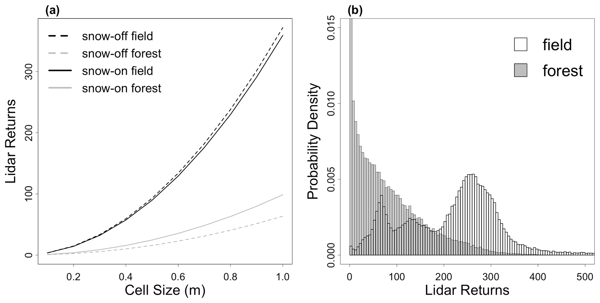
Figure 2(a) Average lidar point cloud density of the ground returns versus cell size by land cover and snow-on and snow-off state. (b) Probability density function for the number of lidar ground returns by square meter for the forest (gray) and the field (white).
3.2 Lidar and in situ snow depth comparison
Based on the magnaprobe snow depth and UAS-mapped snow depth measurements, the accuracy of lidar snow depth measurements differed between field and forest cells (Fig. 3). In the field, the mean snow depth from the magnaprobe (12.2 cm ± 0.56 cm) was only slightly greater than that from the lidar (11.2 cm ± 0.72 cm), and the MAD and RMSD values were 0.96 cm and 1.22 cm, respectively. In the forest, the mean snow depth from the magnaprobe (15.2 cm ± 2.3 cm) was twice as large as the lidar snow depths (7.8 cm ± 6.3 cm), and the MAD and RMSD were 9.6 and 10.5 cm, respectively. The mean snow depth from the Federal snow tube was 12.9 cm ± 0.71 cm and 13.1 cm ± 1.9 cm in the field and forest, respectively. There is a notable absolute low bias in the lidar forest snow depth relative to the magnaprobe and snow tube for the western forest in particular, with the exception of one site.
To provide insight into differences between the forest and field observations, height profiles of classified returns were calculated for 25 m2 square regions centered on all forest (n=12) and field (n=7) study plots from lidar data. Height profiles were averaged for each site type, from here on referred to as mean height profiles (Fig. 4). To do this, all lidar returns were extracted from the bounding box of each plot, and then the mean elevation of ground returns was calculated within each plot. Return height profiles for each plot were determined by subtracting the mean ground elevation of the plot from each return, and then the normalized return elevations were binned in 0.1 m height increments. Within the forests, an average of 2142 and 2889 returns were classified as ground and non-ground, respectively, in snow-free conditions for each 25 m2 plot. Snow-on conditions had a comparable number of ground returns (2218) but fewer non-ground returns (1721). In field plots, an average of 5666 ground returns and 154 non-ground returns in snow-free conditions were obtained for each 25 m2 plot, with 7567 ground returns and 25 non-ground returns in snow-on conditions. Figure 4 also shows that there is a greater range of ground return elevations in the forest as compared to the field. In forest plots, ground return elevations had an average standard deviation of 0.157 and 0.154 m in snow-free and snow-on conditions, respectively, while in field plots, ground return elevations had standard deviations of 0.058 and 0.050 m in snow-free and snow-on conditions, respectively.
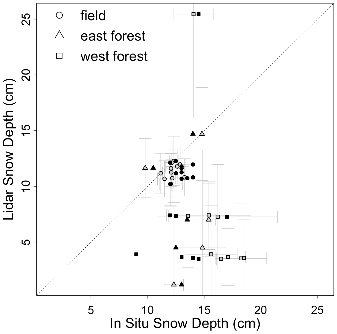
Figure 3Comparison between the magnaprobe (gray fill) and snow tube (black fill) versus the lidar snow depth measurements by location. The mean and 95 % confidence intervals were calculated using the five magnaprobe snow depths and the lidar snow depths (Eq. 1), averaged over a 0.4 m × 0.4 m grid cell. Individual snow-tube snow depth measurements are shown without confidence intervals.
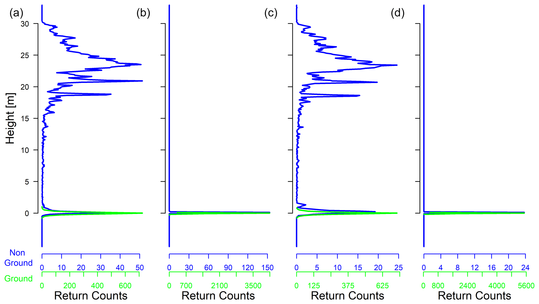
Figure 4Mean height profiles for all ground (green) and non-ground (blue) lidar returns within a 5 m × 5 m region centered on each transect plot in snow-free conditions (a, b) and snow-on conditions (c, d) in forest (a, c) and field (b, d) study plots.
3.3 Snow depth maps from UAS lidar
The UAS-mapped snow depth, mapped by subtracting snow-off DTMs from snow-on DTMs, revealed a shallow snowpack whose depth ranges from less than 2 to over 18 cm (Fig. 5). The mean lidar snow depth was 10.3 cm in the field and 6.0 cm in the forest. Despite the shallow conditions, spatially coherent patterns are readily discernible. The field snowpack depth had higher spatial variability than the western forest snowpack and more spatial organization. In the field, the deepest snow was in the low-lying northeastern areas that are sheltered from westerly winds. A relatively moderate and consistent snowpack occurred in the southern part of the eastern field and west of the small pond. The shallowest snowpack was found in the center portion of the field, which is slightly elevated and, unlike most of the field, was not mowed. Lower snow depth at the forest edge distinguishes the field-to-forest transition. A non-parametric Steel–Dwass test found significant variation for the mean snow depth among the two forest types and field (p < 0.0001) (Fig. 6a). Figure 6a and b also reveal that there are some negative snow depths in the two forest types that are due to the uncertainty in the snow-on and snow-off DTMs.
A pairwise Steel–Dwass test showed that snow depths were significantly different between the three pairs of field and forest types (p < 0.0001). When comparing just field and forest as categories, the test also found significant differences for snow depth (p < 0.0001). Snow depth was also determined to be significantly different among the three slope group categories using the Steel–Dwass test, where regions with a limited slope (Group 1) had more decidedly different snow than steeper regions (p < 0.0001) (Fig. 6b).
The values of the one-sided confidence interval of the mean snow depth estimate are remarkably consistent in the field and typically are between 0.5 1 cm regardless of snow depth (Fig. 5b). Modestly larger confidence intervals occur adjacent to the north–south road, where the fields were not mowed prior to winter, as well as the northern and southern extents of the flight lines, likely due to the reduced sampling density. The forest had an average one-sided confidence interval of 3.5 cm, which was considerably higher than the field. Where the forest is predominantly comprised of deciduous trees, the typical one-sided confidence intervals of the mean snow depth were as low as 1 to 2 cm. The largest one-sided confidence intervals occurred in the middle of the field, where there was dense shrubbery; at the edge of the fields; and in clusters within the forest where the forest sections were dominated by coniferous trees (Pinus strobus). The nexus of flight lines in the take-off and landing area resulted in a local area with very high confidence. A non-parametric Steel–Dwass test found significant variation for confidence intervals of the mean snow depth among the two forest types and field (p < 0.0001) (Fig. 6c). A pairwise Steel–Dwass test showed that confidence intervals were significantly different among the three pairs of field and forest types (p < 0.0001). Confidence intervals were also significantly different among the three slope categories, as determined using a Steel–Dwass test (p < 0.0001) (Fig. 6d).
3.4 Point cloud density, spatial resolution, and canopy profiles
Confidence intervals for the mean snow depths by grid cell were examined in light of the point cloud density and the spatial resolution at which lidar returns were aggregated. The confidence interval width for a mean snow depth of a 1 m2 area decreased dramatically as the lidar point cloud density increased (Fig. 7a). Except for the cells with fewer than 10 points/m2, forest cells had larger confidence intervals for the mean depths than field cells for a given sample size. When the density exceeds 25 points/m2 in the field and 50 points/m2 in the forest, confidence intervals were typically 2 cm. The cells with the highest point cloud densities had one-sided confidence intervals of about 1 and 1.5 cm for the field and forest cells, respectively. The field cells with more than 50 points/m2 did not have noticeably smaller confidence intervals, but the increased density did reduce the number of cells with anomalously small confidence intervals. Given the high lidar point cloud density for the field cells, it is possible that reasonable estimates of snow depth can be made at scales finer than 1 m (Fig. 7b).
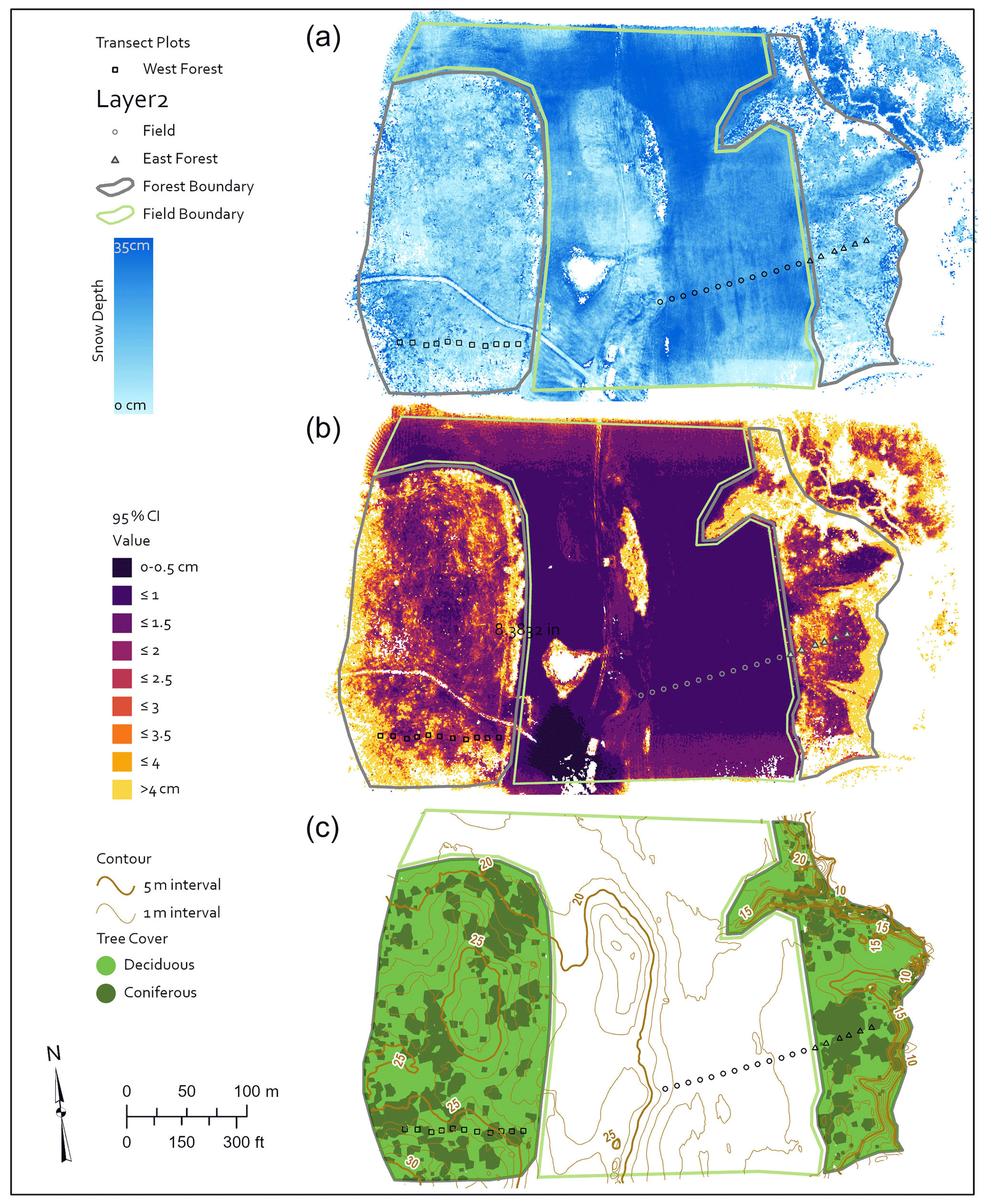
Figure 5Average (a) snow depth values, (b) one-sided confidence intervals, and (c) topography and forest cover type. Snow depth and confidence intervals calculated from the snow-on and snow-off lidar point clouds for 1 m2 cells at Thompson Farm, Durham, NH. Topography and forest cover type determined from snow-off lidar point clouds on snow-off flight for 1 m2 cells conducted on 11 April 2019.
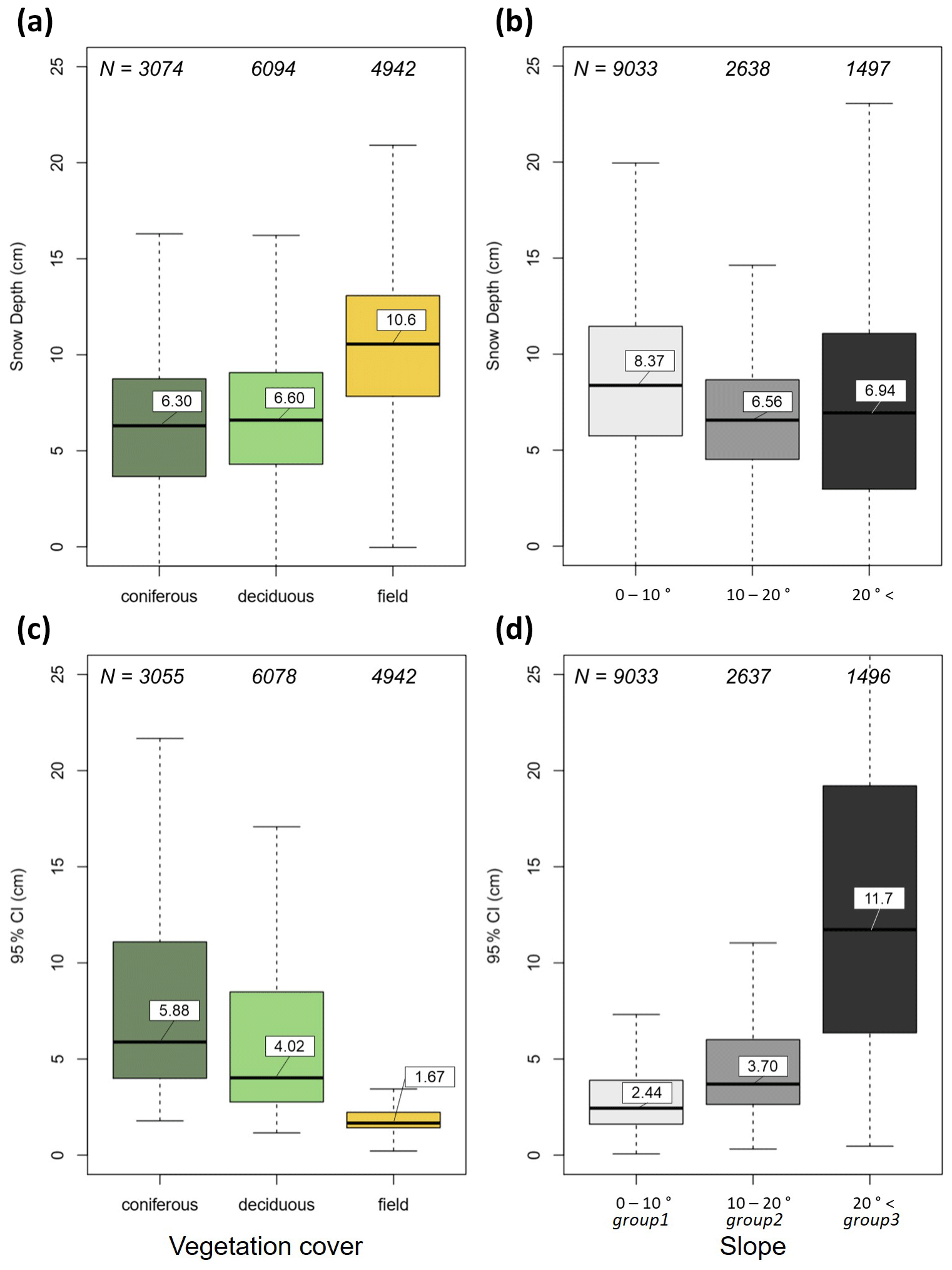
Figure 6Snow depths (a, b) and their one-sided confidence intervals (c, d) from the random sample points of the field and forest at Thompson Farm, Durham, NH, on 23 January 2019 from the individual cells for 1 m2 cells by vegetation cover (a, c) and slope group (b, d). Boxplots show the lower quartile, median, upper quartile, and whiskers with the median value noted. Because of missing values in the raster images, not all random points extracted values and resulted in different numbers of sample points for vegetation cover classes.

Figure 7One-sided confidence intervals of the mean snow depth values in the field and forest at Thompson Farm, Durham, NH, on 23 January 2019 from the individual cells for 1 m2 cells by land cover and point cloud density (a) and for grid resolutions ranging from 0.1 to 5 m (b). Boxplots show the lower quartile, median, upper quartile, and whiskers.
In addition to the lidar point cloud density, the ability to reduce the confidence interval of the mean snow depth also depends on the ground surface variability within a cell as well as the lidar performance. For this site and its shallow snowpack, the grid cell variability in the ground surface elevation, estimated by calculating the standard deviation of the lidar elevation values, is found to depend primarily on the cell size and, to a more limited extent, on land cover and snow cover (Fig. 8a). Snow cover reduced the grid cell variability in the field by about 1 cm but has a limited effect in the forest. It is possible that the modest snowpack was able to flatten the higher grass in the field, while the forest's vegetation and ground surface features that dominate the grid cell variability were only minimally compacted by the snow. Within the 1 m grid cells, snow depth variability was much lower in the field than the forest (Fig. 8b). Both distributions had a positive skew. Typical standard deviations of the lidar surface elevation values within a 10 cm cell were on the order of 1.5 and 2 cm for the field and forest, respectively. That variability doubled for a 20 cm cell. The grid cell variability increased gradually to about 3 to 4 cm in the field and to about 6 cm in the forest.
Thus, confidence intervals largely depended on the point cloud density in the lidar cloud because the standard deviation of a cell's surface elevation is relatively constant for snow depth resolutions from 0.5 to 1 m (Fig. 8a). In the field, reducing the cell size from 1 to 0.5 m still yields about 100 points/m2 and provides snow depth estimates within ±1.5 cm. Because the forest cells required a higher ground return density to capture these snow depths within 1 cm, any reduction in cell size below 1 m greatly increased the confidence intervals of the cells' mean snow depth.
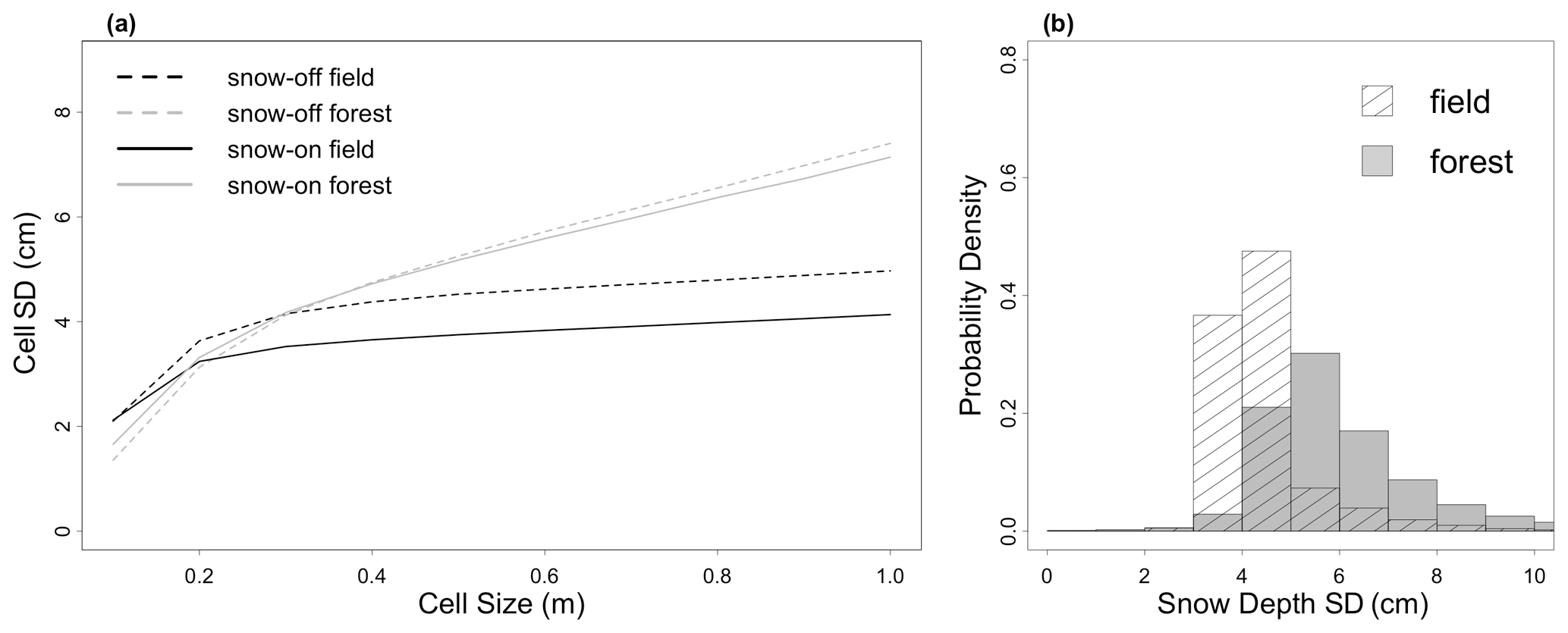
Figure 8Lidar surface elevation standard deviations by (a) cell size and land cover. Cell standard deviations are the average of the individual cells' standard deviation values calculated for cells with side dimensions ranging from 0.1 to 1.0 m. (b) Probability density function of the snow depth's pooled standard deviation for each 1 m2 cell in the forest (gray) and field (hashed).
Despite UAS-based lidar's increasing use in the natural sciences and capacity to make high-resolution snow maps, there are many operational and technical challenges that require consideration prior to successfully conducting UAS-based lidar surveys that produce research-grade, high-resolution snow depth data. For the lidar surveys, the hardware and supporting software analysis tools can be expensive and require trained pilots and lidar data analysis specialists. In this section, we present some general considerations regarding validation of the lidar snow depth maps, selection, and deployment of a lidar sensor on a UAV for snow depth mapping as well as specific insights that we experienced when using our system.
4.1 In situ and UAS sampling
This study's lidar snow depth performance metrics are comparable to those from the more extensive lidar surveys made by Harder et al. (2020). In the field, our snow depth errors, 1 cm bias and 1.2 cm RMSD, were modestly better than those from their open-site snow depth, with a 3 cm bias and RMSE values on the order of 10 cm. In the forest, our snow depth errors, 7 cm bias and 10 cm RMSD, were also modestly lower than those from their forest sites, with a 9 to 13 cm bias and 15 cm RMSE. While it is difficult to make direct comparison across different study sites, snow conditions, and ground validation approaches, these early findings indicate that UAS lidar has the capability of mapping snow depths in open and forested regions and has improved performance as compared to previous SfM results, particularly for vegetated surface. It is also noteworthy that this study's mapping was conducted using the Velodyne Puck series, a laser scanner adapted from the assisted- and autonomous-vehicle applications rather than the specialized Riegl miniVUX-1UAV used by Harder et al. (2020), resulting in a complete mapping system that was approximately one-third the costs of their Riegl system.
While UAS-based lidar surveys can measure snow depth to within a centimeter at high spatial resolutions, validation of those observations is challenging. A time-consuming collection of high-accuracy GNSS survey points was required to co-locate magnaprobe and lidar observations. Surveying and marking sample locations prior to the winter season might reduce this effort. However, the use of sampling stakes risks modifying snow processes at the sample locations and potentially biasing the snowpack and incurring destructive sampling impacts if the same location is being repeatedly visited over a season. It is also challenging to make in situ snow depth measurements that provide centimeter accuracy. In this study, the magnaprobe in situ snow depth observations made in the forest were considerably higher than the lidar observations as compared to the open field, where the magnaprobe and lidar measurements were within 1 cm. Previous studies also found that snow depth observations from ALS measurements are biased lower than those from snow probe observations in the forest (Hopkinson et al., 2004, Currier et al., 2019; Harder et al., 2020). In past studies, the causes of these differences have been partially attributed to the snow probe's ability to penetrate the soil and vegetation, human observers tending to make snow depth measurements in locations with relatively high snow (Sturm and Holmgren, 2018), and the reduced accuracy of the GNSS in the forest. Our study suggests additional issues in forest sampling, including enhanced ground surface variability in forested areas relative to adjacent field areas and reduced lidar returns in forested areas as compared to field areas, combined with sampling issues, to contribute to the higher uncertainty in the forest snow depths observed in our study.
In this study, the cold temperatures and snow-free conditions prior to the 19 and 20 January 2019 snowfall event resulted in deeper frozen soils (23.5 to 25.5 cm) in the field and shallower soil frost depth (5.5 to 8.5 cm) in the western forest, which would have limited the probe penetration into soils at both sites. However, the forest has a 1–4 cm thick leaf litter layer that may have been penetrated by the magnaprobe. The average Federal snow sampler tube depths (13.1 cm) were not as deep as the magnaprobe (15.2 cm) and thus more closely match the lidar snow depth (7.8 cm; see Fig. 3), though a considerably low bias (∼ 5.3 cm) similar to that found by Harder et al. (2020) persists in the lidar snow depth relative to the Federal snow sampler snow depths. Additional factors such as downed logs, thick understory, and fine-scale topographic features (i.e., small boulders and hummocky terrain) as well as reduced ground return density may contribute to the lidar snow depth errors in a forest, whereas these factors are absent in the field.
An improved understanding of forest canopy impacts on lidar returns is also warranted. Recent work has demonstrated that lidar pulses are “lost” at a much higher rate in forest canopies than open ground due to interception, absorption, and scattering through canopy transmission, with the loss ratio largely influenced by the range of the target from the sensor (Liu et al., 2020). The data that we present in this paper were acquired using constant flight speed and at a consistent altitude above target areas. Because of this, it is feasible that forest canopy conditions and variable understory vegetation density may have resulted in lost pulses and increased uncertainty in our data set. Indeed, we did observe lower return densities for both ground and all returns in forested areas in our data set (Fig. 4).
One possible outcome of these lidar sampling issues in forests was a significant difference in snow depth confidence intervals between field and forest types and among slope groups. Confidence intervals were highest in conifer stands and on steep slopes and lowest in the field. This is likely partially the result of lower ground return density in forests due to the combined effects of lost pulses and canopy occlusion in forested areas. Additionally, this observation may be driven by increased variability in snow-off ground surface due to higher variability in the subnivean terrain in the forested areas of the study site (e.g., pockets of duff and woody debris). On cells where slopes exceed 20∘, there is more variability in ground return elevations over shorter distances due to errors in horizontal directions and spreading of the laser spot (Deems et al., 2013), which would partially drive larger confidence intervals of ground surface elevation for pixels located in high-relief areas. These relatively high-slope areas were more common in forested areas of the study site, and the DTM uncertainty resulting when there are high slopes also carries through snow depth estimation. Snow depth was significantly different between field and forested areas as well as between conifer and deciduous forest types, despite the relatively high uncertainty. This indicates the possible influence of tree canopies on snow accumulation due to enhanced snow interception in forests (see reviews in Clark et al., 2011) and particularly in conifer stands but also could be the result of an under-sampled ground surface in forested areas relative to field areas. Despite challenges with sampling in the forest area, some degree of coherence for snow depth in the forest is apparent. The forest interception effects may be captured on average through forest structure parameters such as canopy closure and leaf area index that have traditionally been used in snow models with canopy–snow interactions (see reviews in snow model inter-comparison project – SNOWMIP2 by Essery et al., 2009; Rutter et al., 2009). However, the finer-scale heterogeneity may benefit from additional parameters such as the mean distance to canopy and total gap area (Moeser et al., 2016) or modifications that reflect variations in canopy structure (Mazzotti et al., 2019). Snow depth was also significantly different among the three slope groups, possibly due to wind-driven snow displacement and sloughing on slopes during accumulation.
4.2 Flight planning
Because high-lift UAVs capable of carrying a lidar sensor package have challenges that may differ from small consumer-grade UAVs used mainly for optical-photogrammetry surveying, a well-formulated flight plan that addresses weather conditions, logistics of flying at a proposed site, flight lines, UAS equipment, and personnel is clearly needed. Weather impacts operations. UAS surveys cannot be conducted when there is any type of precipitation or in dense fog or clouds because moisture can cause electronic components to malfunction, and moisture build-up on the propellers can also adversely affect lift production. Depending on the UAS, wind speeds exceeding 7 to 10 m/s may make flights more difficult. This project's Eagle XF high-lift-capacity UAV cannot be flown comfortably in winds greater than 8 m/s. At the study site, wind speeds often exceeded this threshold on the days immediately following snowfall except early in the morning. High wind speeds can also significantly reduce battery life as well as impact the accuracy of sensor observations. Low air temperatures can cause batteries to rapidly discharge. For winter UAS surveys, all flight and operational batteries were kept warm in a building, vehicle, or insulated cooler prior to the UAS survey. This also applies to the computer used to upload flight lines and relay telemetry information. A MIL-STD-810-certified Panasonic Toughbook was used in this study to handle the anticipated cold temperatures. Additionally, cold temperatures can severely limit the dexterity of the person manipulating the flight controls.
These high-lift UAVs also have the potential to cause significant damage to person and property. The selection of a survey site not only needs to meet the scientific objectives of the UAS lidar survey but also must have the proper attributes for safe and legal UAV operation including permission to operate the UAV at the site. Visual line of sight (VLOS) of the UAS needs to be maintained throughout the flight. When it is difficult to maintain VLOS (e.g., flying over forested or mountainous sites), spotters can be used if there is constant two-way communication between the spotters and the person operating the flight controls. For this study, an on-site walk-up tower with a spotter was necessary while the UAS was flown over the forest.
The deployment of a UAS lidar requires additional flight patterns designed for boresighting to ensure that point clouds are aligned (Painter et al., 2016). Provided that GNSS data are accurate, the most common reason for misalignment of point clouds is boresight angle errors (Li et al., 2019). Boresighting is the process of calculating the differences between lidar sensor and IMU (inertial measurement unit) roll, pitch, and yaw angle measurements to correct those errors in point clouds. Due to battery flight time limitations, we were unable to complete the flight pattern that is commonly used for boresighting alignment. Because of this, we leveraged our first two antiparallel flight lines for boresighting calibration. Additional details on boresighting calibration, our technique due to the flight time limitations, and examples of roll and pitch alignment errors observed during this field campaign appear in the Supplement.
4.3 UAS sampling strategies
While lidar calibration and data post-processing requirements are quite similar for UAS and airborne surveys, the UAS lidar surveys presented in this study have key differences from previous ALS surveys. As noted above, UAS flight durations are considerably shorter, resulting in limited spatial coverage as compared to previous ALS snow depth surveys. This study took approximately 2 h to map a 0.1 km2 area. An advantage of UAS over ALS surveys is that the average point cloud density is much higher and has fewer missing pixels in the forest. This study's sampling densities and the proportion of areas with no ground returns are quite different from previous airborne lidar snow depth studies. This study had ground returns of 90 and 364 points/m2 in the forest and field, respectively, and had no ground returns in only 0.086 % and 0.95 % of the 1 m resolution field and forest cells, respectively. In contrast, ALS surveys typically report surface model densities between 8 and 16 points/m2 (Broxton et al., 2015, 2019; Currier et al., 2019; Kirchner et al., 2014) and ground returns between 3 and 6 points/m2 (Broxton et al., 2019; Kirchner et al., 2014). ALS-derived snow depth maps have a much greater proportion of areas that are masked due to no ground returns, particularly under trees, with masking areas ranging from less than 10 % to more than 23 % (Harpold et al., 2014; Mazzotti et al., 2019). While gap filling is possible, interpolation using measured snow depth values to fill under trees can overestimate snow depth (Zheng et al., 2016). Based on our work comparing field and forest lidar collections from a UAS, we suggest testing alternative flight plans, including reduced flight speed over forest canopies to account for lost pulses and canopy returns to produce ground return density that is comparable to field ground return density and to further reduce the number of missing pixels in an acquisition area. It is worth noting that as the capabilities of UAVs, power supplies, and lightweight sensors continue to advance at an accelerated rate, UAS platforms will shortly rival the spatial coverage attainable by manned aircraft while maintaining improved efficiency and cost effectiveness.
A well-understood challenge exists when developing a spatial-sampling strategy in which, for given resources, there is a trade-off between spatial extent and sampling density (Clark et al., 2011). Increasing flight altitude can expand the spatial extent of an aerial survey. However, flying at higher altitudes results in a decreased point density. In theory, a higher point density could be achieved by slower speeds and increased swath overlap. The targeted spatial extent of an aerial survey dictates whether a manned aircraft or a UAV should be used. If the targeted area has a limited domain, then using a manned airborne platform is probably overkill and inefficient for many studies, and the use of a UAV would be more cost-effective. However, as the domain increases in size, additional batteries would be required, much of the battery power would be used to reach the outer limits of the domain, and the ability to maintain the required line of sight could be difficult. Thus, there are end-members for survey sites or regions where it is self-evident as to whether a UAV or an airborne platform should be used, but that leaves considerable gray areas where an appropriate choice of UAV platform with a well-designed mission could stretch the domain. Future research and technological advances are needed to offer insights for snow science observation platforms and trade-offs.
This paper describes and demonstrates a UAS-based lidar survey for snow depth mapping using commercially available components. The snow depth map was assessed in a mixed deciduous and coniferous forest and open field with little relief over a thin snowpack. The UAS includes an Eagle XF UAV manufactured by UAV America, a small, lightweight VLP-16 lidar (Velodyne, Inc.), and an Applanix APX-15 UAV INS. The INS has a measurement rate of 200 Hz, allowing returns to be georeferenced without ground control points. Data, post-processed to an SBET file, resulted in approximately 3 cm positional accuracy. Flights were conducted at an altitude of 81 m and flight speed of 7 m/s, with a total of 12 parallel flight lines with targeted overlap of 40 %. Once the point clouds were classified as ground and non-ground points, the flights yielded an average of 90 and 364 ground points/m2 in the forest canopy and field, respectively, with 6.7 % of the forest and 0.03 % of the field cells having fewer than 5 points/m2.
The snow depth map, generated by subtracting snow-off from snow-on DTMs derived from the resultant point clouds, reveals a snowpack whose depth ranges from less than 2 to over 18 cm. For both snow depth and confidence intervals, differences were found between vegetation cover types and slope, indicating complex snow–vegetation interaction that can be observed by UAS lidar return numbers. For 0.4 m × 0.4 m cells, the in situ and lidar mean snow depths in the field were nearly identical, with MAD and RMSD values of approximately 1 cm. In the forest, the in situ mean snow depths from a magnaprobe were twice as large as the lidar snow depths, with a correspondingly high RMSD. These forest differences have numerous possible explanations: (1) the snow probe's ability to penetrate the soil and vegetation resulting in random errors; (2) higher uncertainty in areas with canopy cover, variable ground surface, and high slope that occur more commonly in forested areas; (3) reduced total and ground return density in forests due to occlusion and lost pulses. Nevertheless, the results support previous findings indicating that there are limits to lidar snow depth validation at high horizontal and vertical spatial resolutions in some land covers and conditions. Mapped with 1 m2 cells, a 0.5 to 1 cm snow depth confidence interval was achieved consistently in the field, with confidence intervals increasing to median values of 4.0 cm in the deciduous forest and 5.9 cm in the coniferous forest. In the field, snow depth can be mapped at finer spatial resolutions with limited reduction in performance when reducing the cell size to 0.5 m × 0.5 m and still achieve snow depth confidence intervals of less than 5 cm for a 0.2 m × 0.2 m cell size. Performance depends on both the point cloud density, which can be increased or decreased by changing the flight plan, and the grid cell variability that depends on site surface conditions.
The UAS-based lidar point clouds and in situ snow observations are available from the corresponding author upon reasonable request.
The supplement related to this article is available online at: https://doi.org/10.5194/tc-15-1485-2021-supplement.
JMJ, AGH, FBS, and MP designed research and performed analysis. JMJ, AGH, FBS, MP, EAB, and EC conducted fieldwork to obtain lidar and/or in situ snow observations. AGH, FBS, CH, and EC produced figures. JMJ wrote the initial draft. All authors contributed to manuscript review and editing.
The authors declare that they have no conflict of interest.
This material is based upon work supported by the Broad Agency Announcement Program and the Cold Regions Research and Engineering Laboratory (ERDC-CRREL) under contract number W913E5-18-C-005. Any opinions, findings, and conclusions or recommendations in this material are those of the author(s) and do not necessarily reflect the views of the Broad Agency Announcement Program and the Cold Regions Research and Engineering Laboratory.
The authors are grateful to Lee Friess for providing a technical review of the draft manuscript, Mahsa Moradi Khaneghahi for supporting manuscript preparation, and Ronny Schroeder for contributing to the field data collection.
This research has been supported by the Broad Agency Announcement Program and the Cold Regions Research and Engineering Laboratory (grant no. W913E5-18-C-005).
This paper was edited by Philip Marsh and reviewed by four anonymous referees.
Adams, M. S., Bühler, Y., and Fromm, R.: Multitemporal accuracy and precision assessment of unmanned aerial system photogrammetry for slope-scale snow depth maps in Alpine terrain, Pure Appl. Geophys., 175, 3303–3324, 2018.
Broxton, P., Harpold, A., Biederman, J., Troch, P. A., Molotch, N., and Brooks, P.: Quantifying the effects of vegetation structure on snow accumulation and ablation in mixed-conifer forests, Ecohydrology, 8, 1073–1094, 2015.
Broxton, P. D., van Leeuwen, W. J., and Biederman, J. A.: Improving Snow Water Equivalent Maps With Machine Learning of Snow Survey and Lidar Measurements, Water Resour. Res., 55, 3739–3757, https://doi.org/10.1029/2018wr024146, 2019.
Bühler, Y., Adams, M. S., Bösch, R., and Stoffel, A.: Mapping snow depth in alpine terrain with unmanned aerial systems (UASs): potential and limitations, The Cryosphere, 10, 1075–1088, https://doi.org/10.5194/tc-10-1075-2016, 2016.
Bühler, Y., Adams, M. S., Stoffel, A., and Boesch, R.: Photogrammetric reconstruction of homogenous snow surfaces in alpine terrain applying near-infrared UAS imagery, Int. J. Remote Sens., 38, 3135–3158, 2017.
Burakowski, E., Tawfik, A., Ouimette, A., Lepine, L., Novick, K., Ollinger, S., Zarzycki, C., and Bonan, G.: The role of surface roughness, albedo, and Bowen ratio on ecosystem energy balance in the Eastern United States, Agr. Forest Meteorol., 249, 367–376, 2018.
Burakowski, E. A., Ollinger, S. V., Lepine, L., Schaaf, C. B., Wang, Z., Dibb, J. E., Hollinger, D. Y., Kim, J., Erb, A., and Martin, M.: Spatial scaling of reflectance and surface albedo over a mixed-use, temperate forest landscape during snow-covered periods, Remote Sens. Environ., 158, 465–477, 2015.
Cimoli, E., Marcer, M., Vandecrux, B., Bøggild, C. E., Williams, G., and Simonsen, S. B.: Application of low-cost UASs and digital photogrammetry for high-resolution snow depth mapping in the Arctic, Remote Sens., 9, 1144, https://doi.org/10.3390/rs9111144, 2017.
Clark, M. P., Hendrikx, J., Slater, A. G., Kavetski, D., Anderson, B., Cullen, N. J., Kerr, T., Örn Hreinsson, E., and Woods, R. A.: Representing spatial variability of snow water equivalent in hydrologic and land-surface models: A review, Water Resour. Res., 47, W07539, https://doi.org/10.1029/2011wr010745, 2011.
Cook, B. D., Corp, L. A., Nelson, R. F., Middleton, E. M., Morton, D. C., McCorkel, J. T., Masek, J. G., Ranson, K. J., Ly, V., and Montesano, P. M.: NASA Goddard's LiDAR, Hyperspectral and Thermal (G-LiHT) Airborne Imager, Remote Sens., 5, 4045–4066, 2013.
Currier, W. R. and Lundquist, J. D.: Snow depth variability at the forest edge in multiple climates in the western United States, Water Resour. Res., 54, 8756–8773, 2018.
Currier, W. R., Pflug, J., Mazzotti, G., Jonas, T., Deems, J. S., Bormann, K. J., Painter, T. H., Hiemstra, C. A., Gelvin, A., and Uhlmann, Z.: Comparing aerial lidar observations with terrestrial lidar and snow-probe transects from NASA's 2017 SnowEx campaign, Water Resour. Res., 55, 6285–6294, https://doi.org/10.1029/2018wr024533, 2019.
Deems, J. S., Painter, T. H., and Finnegan, D. C.: Lidar measurement of snow depth: a review, J. Glaciol., 59, 467–479, 2013.
De Michele, C., Avanzi, F., Passoni, D., Barzaghi, R., Pinto, L., Dosso, P., Ghezzi, A., Gianatti, R., and Della Vedova, G.: Using a fixed-wing UAS to map snow depth distribution: an evaluation at peak accumulation, The Cryosphere, 10, 511–522, https://doi.org/10.5194/tc-10-511-2016, 2016.
Dickinson, W. and Whiteley, H.: A sampling scheme for shallow snowpacks, Hydrol. Sci. J., 17, 247–258, 1972.
Dolgun, A. and Demirhan, H.: Performance of nonparametric multiple comparison tests under heteroscedasticity, dependency, and skewed error distribution, Commun. Stat. Simulat., 46, 5166–5183, 2017.
Eberhard, L. A., Sirguey, P., Miller, A., Marty, M., Schindler, K., Stoffel, A., and Bühler, Y.: Intercomparison of photogrammetric platforms for spatially continuous snow depth mapping, The Cryosphere, 15, 69–94, https://doi.org/10.5194/tc-15-69-2021, 2021.
Essery, R., Rutter, N., Pomeroy, J., Baxter, R., Stähli, M., Gustafsson, D., Barr, A., Bartlett, P., and Elder, K.: SNOWMIP2: An evaluation of forest snow process simulations, B. Am. Meteorol. Soc., 90, 1120–1136, 2009.
Fernandes, R., Prevost, C., Canisius, F., Leblanc, S. G., Maloley, M., Oakes, S., Holman, K., and Knudby, A.: Monitoring snow depth change across a range of landscapes with ephemeral snowpacks using structure from motion applied to lightweight unmanned aerial vehicle videos, The Cryosphere, 12, 3535–3550, https://doi.org/10.5194/tc-12-3535-2018, 2018.
Fey, C., Schattan, P., Helfricht, K., and Schöber, J.: A compilation of multitemporal TLS snow depth distribution maps at the Weisssee snow research site (Kaunertal, Austria), Water Resour. Res., 55, 5154–5164, https://doi.org/10.1029/2019WR024788, 2019.
Gabrlik, P., Janata, P., Zalud, L., and Harcarik, J.: Towards Automatic UAS-Based Snow-Field Monitoring for Microclimate Research, Sensors, 19, 1945, https://doi.org/10.3390/s19081945, 2019.
Gandahl, R.: Determination of the depth of soil freezing with a new frost meter, Report 30 (SIP 16347), Stattensaginsititut, Stockholm, Sweden, 1957 (in Swedish).
Goetz, J. and Brenning, A.: Quantifying uncertainties in snow depth mapping from structure from motion photogrammetry in an alpine area, Water Resour. Res., 55, 7772–7783, 2019.
Grünewald, T., Schirmer, M., Mott, R., and Lehning, M.: Spatial and temporal variability of snow depth and ablation rates in a small mountain catchment, The Cryosphere, 4, 215–225, https://doi.org/10.5194/tc-4-215-2010, 2010.
Harder, P., Schirmer, M., Pomeroy, J., and Helgason, W.: Accuracy of snow depth estimation in mountain and prairie environments by an unmanned aerial vehicle, The Cryosphere, 10, 2559–2571, https://doi.org/10.5194/tc-10-2559-2016, 2016.
Harder, P., Pomeroy, J. W., and Helgason, W. D.: Improving sub-canopy snow depth mapping with unmanned aerial vehicles: lidar versus structure-from-motion techniques, The Cryosphere, 14, 1919–1935, https://doi.org/10.5194/tc-14-1919-2020, 2020.
Harpold, A., Guo, Q., Molotch, N., Brooks, P., Bales, R., Fernandez-Diaz, J., Musselman, K., Swetnam, T., Kirchner, P., and Meadows, M.: LiDAR-derived snowpack data sets from mixed conifer forests across the Western United States, Water Resour. Res., 50, 2749–2755, 2014.
Helsel, D. R. and Hirsch, R. M.: Statistical methods in water resources, Elsevier, Reston, VA, 2002.
Hopkinson, C., Chasmer, L., Young-Pow, C., and Treitz, P.: Assessing forest metrics with a ground-based scanning lidar, Can. J. Forest Res., 34, 573–583, 2004.
Horn, B. K.: Hill shading and the reflectance map, Proceedings of the IEEE, 69, 14–47, 1981.
Kirchner, P. B., Bales, R. C., Molotch, N. P., Flanagan, J., and Guo, Q.: LiDAR measurement of seasonal snow accumulation along an elevation gradient in the southern Sierra Nevada, California, Hydrol. Earth Syst. Sci., 18, 4261–4275, https://doi.org/10.5194/hess-18-4261-2014, 2014.
Kraus, K. and Pfeifer, N.: Advanced DTM generation from LiDAR data, ISPRS Archives, 34, 23–30, 2011.
Li, Z., Tan, J., and Liu, H.: Rigorous boresight self-calibration of mobile and UAV LiDAR scanning systems by strip adjustment, Remote Sens., 11, 442, https://doi.org/10.3390/rs11040442, 2019.
Liu, Q., Fu, L., Wang, G., Li, S., Li, Z., Chen, E., Pang, Y., and Hu, K.: Improving Estimation of Forest Canopy Cover by Introducing Loss Ratio of Laser Pulses Using Airborne LiDAR, IEEE T. Geosci. Remote, 58, 567–585, https://doi.org/10.1109/TGRS.2019.2938017, 2020.
Marti, R., Gascoin, S., Berthier, E., de Pinel, M., Houet, T., and Laffly, D.: Mapping snow depth in open alpine terrain from stereo satellite imagery, The Cryosphere, 10, 1361–1380, https://doi.org/10.5194/tc-10-1361-2016, 2016.
Maune, D. F. and Nayegandhi, A.: Digital elevation model technologies and applications: the DEM users manual, Asprs Publications, Bethesda, Maryland, 2018.
Mazzotti, G., Currier, W. R., Deems, J. S., Pflug, J. M., Lundquist, J. D., and Jonas, T.: Revisiting Snow Cover Variability and Canopy Structure Within Forest Stands: Insights From Airborne Lidar Data, Water Resour. Res., 55, 6198–6216, 2019.
McGrath, D., Webb, R., Shean, D., Bonnell, R., Marshall, H. P., Painter, T. H., Molotch, N. P., Elder, K., Hiemstra, C., and Brucker, L.: Spatially extensive ground-penetrating radar snow depth observations during NASA's 2017 SnowEx campaign: Comparison with In situ, airborne, and satellite observations, Water Resour. Res., 55, 10026–10036, 2019.
Meyer, J. and Skiles, S. M.: Assessing the Ability of Structure From Motion to Map High-Resolution Snow Surface Elevations in Complex Terrain: A Case Study From Senator Beck Basin, CO, Water Resour. Res., 55, 6596–6605, 2019.
Moeser, D., Mazzotti, G., Helbig, N., and Jonas, T.: Representing spatial variability of forest snow: Implementation of a new interception model, Water Resour. Res., 52, 1208–1226, 2016.
Mott, R., Schirmer, M., and Lehning, M.: Scaling properties of wind and snow depth distribution in an Alpine catchment, J. Geophys. Res.-Atmos., 116, D06106, https://doi.org/10.1029/2010jd014886, 2011.
Mott, R., Vionnet, V., and Grünewald, T.: The seasonal snow cover dynamics: review on wind-driven coupling processes, Front. Earth Sci., 6, 197, https://doi.org/10.3389/feart.2018.00197, 2018.
Muir, J., Goodwin, N., Armston, J., Phinn, S., and Scarth, P.: An accuracy assessment of derived digital elevation models from terrestrial laser scanning in a sub-tropical forested environment, Remote Sens., 9, 843, https://doi.org/10.3390/rs9080843, 2017.
Nolan, M., Larsen, C., and Sturm, M.: Mapping snow depth from manned aircraft on landscape scales at centimeter resolution using structure-from-motion photogrammetry, The Cryosphere, 9, 1445–1463, https://doi.org/10.5194/tc-9-1445-2015, 2015.
Painter, T. H., Berisford, D. F., Boardman, J. W., Bormann, K. J., Deems, J. S., Gehrke, F., Hedrick, A., Joyce, M., Laidlaw, R., and Marks, D.: The Airborne Snow Observatory: Fusion of scanning lidar, imaging spectrometer, and physically-based modeling for mapping snow water equivalent and snow albedo, Remote Sens. Environ., 184, 139–152, 2016.
Palace, M., Keller, M., Asner, G. P., Hagen, S., and Braswell, B.: Amazon forest structure from IKONOS satellite data and the automated characterization of forest canopy properties, Biotropica, 40, 141–150, 2008.
Palace, M. W., Sullivan, F. B., Ducey, M. J., Herrick, C.: Estimating Tropical Forest Structure Using a Terrestrial Lidar, PloS ONE, 11, e0154115, https://doi.org/10.1371/journal.pone.0154115, 2016.
Palace, M. W., McMichael, C., Braswell, B. H., Hagen, S. C., Bush, M. B., Neves, E., Tamanaha, E., Herrick, C., and Frolking, S.: Ancient Amazonian populations left lasting impacts on forest structure, Ecosphere, 8, e02035, https://doi.org/10.1002/ecs2.2035, 2017.
Perron, C. J., Bennett, K., and Lee, T. D.: Forest stewardship plan: Thompson farm, NH: University of New Hampshire, Produced by Ossipee Mountain Land Company, West Ossipee, available at: https://unh.app.box.com/s/5jk13l1ektbu57iqb93twx28ldb2anfw (last access: 11 March 2021), 2004.
R Core Team: R: A language and environment for statistical computing, R Foundation for Statistical Computing, Vienna, Austria, available at: https://www.R-project.org/ (last access: 21 March 2021), 2020.
Ricard, J. A., Tobiasson, W., and Greatorex, A.: The field assembled frost gage, Technical Note, Cold Regions Research and Engineering Laboratory, U.S. Army Corps of Engineers, Hanover, New Hampshire, USA, 7 pp., 1976.
Rutter, N., Essery, R., Pomeroy, J., Altimir, N., Andreadis, K., Baker, I., Barr, A., Bartlett, P., Boone, A., and Deng, H.: Evaluation of forest snow processes models (SnowMIP2), J. Geophys. Res.-Atmos., 114, D06111, https://doi.org/10.1029/2008jd011063, 2009.
Schweizer, J., Jamieson, J. B., and Schneebeli, M.: Snow avalanche formation, Rev. Geophys., 41, 25, https://doi.org/10.1029/2002rg000123, 2003.
Sharratt, B. S. and McCool, D. K.: Frost Depth, in: Micrometeorology in Agricultural Systems, in: Micrometeorology in Agricultural Systems, edited by: Hatfield, J. L. and Baker, J. M., Madison, Wisconsin, USA, 584 pp., 2005.
Shaw, T. E., Gascoin, S., Mendoza, P. A., Pellicciotti, F., and McPhee, J.: Snow Depth Patterns in a High Mountain Andean Catchment from Satellite Optical Tristereoscopic Remote Sensing, Water Resour. Res., 56, e2019WR024880, https://doi.org/10.1029/2019wr024880, 2020.
Slotznick, S. P., Sperling, E. A., Tosca, N. J., Miller, A. J., Clayton, K. E., van Helmond, N. A. G. M., Slomp, C. P., and Swanson-Hysell, N. L.: Unraveling the mineralogical complexity of sediment iron speciation using sequential extractions, Geochem. Geophy. Geosy., 21, e2019GC008666, https://doi.org/10.1029/2019gc008666, 2020.
Sturm, M. and Holmgren, J.: An automatic snow depth probe for field validation campaigns, Water Resour. Res., 54, 9695–9701, 2018.
Tonkin, T. N. and Midgley, N. G.: Ground-Control Networks for Image Based Surface Reconstruction: An Investigation of Optimum Survey Designs Using UAV Derived Imagery and Structure-from-Motion Photogrammetry, Remote Sens., 8, 786, https://doi.org/10.3390/rs8090786, 2016.
Vander Jagt, B., Lucieer, A., Wallace, L., Turner, D., and Durand, M.: Snow depth retrieval with UAS using photogrammetric techniques, Geosciences, 5, 264–285, 2015.
Wallace, L., Lucieer, A., Watson, C., and Turner, D.: Development of a UAV-LiDAR system with application to forest inventory, Remote Sens., 4, 1519–1543, 2012.
Wallace, L., Lucieer, A., and Watson, C. S.: Evaluating tree detection and segmentation routines on very high resolution UAV LiDAR data, IEEE T. Geosci. Remote, 52, 7619–7628, 2014.
Zhang, K., Chen, S.-C., Whitman, D., Shyu, M.-L., Yan, J., and Zhang, C.: A progressive morphological filter for removing nonground measurements from airborne LIDAR data, IEEE T. Geosci. Remote, 41, 872–882, 2003.
Zheng, Z., Kirchner, P. B., and Bales, R. C.: Topographic and vegetation effects on snow accumulation in the southern Sierra Nevada: a statistical summary from lidar data, The Cryosphere, 10, 257–269, https://doi.org/10.5194/tc-10-257-2016, 2016.