the Creative Commons Attribution 4.0 License.
the Creative Commons Attribution 4.0 License.
 | 02 Dec 2020
Local-scale variability of snow density on Arctic sea ice
Joshua King
Stephen Howell
Mike Brady
Peter Toose
Chris Derksen
Christian Haas
Justin Beckers
Local-scale variations in snow density and layering on Arctic sea ice were characterized using a combination of traditional snow pit and SnowMicroPen (SMP) measurements. In total, 14 sites were evaluated within the Canadian Arctic Archipelago and Arctic Ocean on both first-year (FYI) and multi-year (MYI) sea ice. Sites contained multiple snow pits with coincident SMP profiles as well as unidirectional SMP transects. An existing SMP density model was recalibrated using manual density cutter measurements (n=186) to identify best-fit parameters for the observed conditions. Cross-validation of the revised SMP model showed errors comparable to the expected baseline for manual density measurements (RMSE = 34 kg m−3 or 10.9 %) and strong retrieval skill (R2=0.78). The density model was then applied to SMP transect measurements to characterize variations at spatial scales of up to 100 m. A supervised classification trained on snow pit stratigraphy allowed separation of the SMP density estimates by layer type. The resulting dataset contains 58 882 layer-classified estimates of snow density on sea ice representing 147 m of vertical variation and equivalent to more than 600 individual snow pits. An average bulk density of 310 kg m−3 was estimated with clear separation between FYI and MYI environments. Lower densities on MYI (277 kg m−3) corresponded with increased depth hoar composition (49.2 %), in strong contrast to composition of the thin FYI snowpack (19.8 %). Spatial auto-correlation analysis showed layered composition on FYI snowpack to persist over long distances while composition on MYI rapidly decorrelated at distances less than 16 m. Application of the SMP profiles to determine propagation bias in radar altimetry showed the potential errors of 0.5 cm when climatology is used over known snow density.
- Article
(4819 KB) - Full-text XML
- BibTeX
- EndNote


The stratified nature of snow on sea ice provides a detailed history of interacting geophysical processes and synoptic-scale input. From its deposition on new ice, to melt in summer, these interactions are dynamic, leading to spatiotemporal heterogeneity at multiple scales. For large portions of the Arctic, early season cyclones drive rapid accumulation followed by sustained periods of cold air temperatures and high winds (Webster et al., 2018). The resulting snowpack is characteristically shallow and subject to sustained temperature gradient metamorphism. Contrasting layers associated with these conditions, namely wind slab and depth hoar, form distinctive features of the winter snowpack (Sturm and Holmgren, 2002). Sequential precipitation and wind events contribute to layered complexity where mass is lost to open water (leads, polynyas), mixed-phase precipitation occurs (melt, ice features), or ice topography acts as an obstruction (drifts and dunes). Although structural similarities exist at synoptic scales (e.g. Warren et al., 1999), few studies have quantified local-scale variability on Arctic sea ice (10 m2; Iacozza and Barber, 1999; Sturm and Holmgren, 2002; Sturm et al., 2006) where layered snow strongly modulates optical and thermal properties at the surface (Ledley et al., 1991; Wu et al., 1999).
Accurate remote sensing observations of sea ice are dependent on spatially distributed knowledge of snow mass (a function of thickness and density). For example, snow thickness represents a significant source of uncertainty in altimetry where isostasy is assumed for retrievals of sea ice thickness (Tilling et al., 2016; Kwok et al., 2019). Radar altimetry estimates of sea ice freeboard must also account for variations in snow density to determine an effective speed of propagation within the medium (Giles et al., 2007; Kwok et al., 2011). It is therefore of interest to develop objective representations of snow on sea ice to quantify potential errors and constrain models. In situ studies form the basis of these representations (Barber et al., 1995; Warren et al., 1999; Sturm and Holmgren, 2002; Kwok and Haas, 2015) and are often extended spatially in model or satellite-based products (Kurtz and Farrell, 2011; Lawrence et al., 2018; Liston, et al., 2018; Petty et al., 2018). Given short length scales of variability, application of these approximations must be handled carefully where errors vary with vertical or horizontal resolution (Kern et al., 2015; King et al., 2015). Additionally, where basin-scale inputs are required, recent changes to the Arctic climate system call into question how representative legacy snow climatologies are for current conditions (Kwok and Cunningham, 2008; Laxon et al., 2013; Webster et al., 2014).
Although there is a need for enhanced representation of snow on sea ice, detailed in situ characterization can be challenging and costly to execute. Traditional snow pits are restricted to a single vertical dimension and require trained operators (i.e. Fierz et al., 2009). Adjacent snow pits or multiple profiles can be arranged to enhance horizontal dimensionality but are cumbersome to execute at scale (Benson and Sturm, 1993; Sturm and Benson, 2004). In many cases, a trade-off between horizontal and vertical resolution is necessary to balance available time with spatial coverage. Recently, penetrometer measurements with the SnowMicroPen (SMP; Schneebeli and Johnson, 1998) were used to address this problem, providing a novel method to rapidly characterize snow structural properties including density (Proksch et al., 2015). The SMP provides millimetre-scale mechanical measurements which can be linked to vertical snow structure through modelling of the penetration process (Marshall and Johnson, 2009; Löwe and van Herijnen, 2012). Taking less than a minute to complete a single vertical profile, there is potential to apply the SMP to snow on sea ice to provide detailed information for radiative transfer or mass balance applications at multiple scales.
In this study, we quantify local-scale variation in snow properties on Arctic sea ice using a combination of snow pit and SMP measurements. SMP profiles are used to extend traditional snow pit analysis to characterize variations in density and stratigraphy at spatial scales of up to 100 m. We validate the SMP density model of Proksch et al. (2015) at sites within the Canadian Arctic Archipelago (CAA) and Arctic Ocean (AO) where adjacent density cutter profiles were collected on first-year and multi-year sea ice (FYI and MYI). The SMP density model is recalibrated using snow pits to identify best-fit parameters for the observed conditions. Traditional snow pit stratigraphy is then used to train a supervised SMP classifier, facilitating evaluation of density by layer type. The calibrated density model and layer-type classifier are applied to an independent set of 613 SMP profiles to discuss snowpack length scales of variability on Arctic sea ice. Finally, we apply the SMP-derived properties to an altimetry application, discussing propagation of errors as related to the observed snow structure.
2.1 Study areas and protocols
The measurements utilized in this study were acquired during two April field campaigns conducted near the time of maximum snow thickness (Fig. 1). The snow measurements coincided with NASA Operation IceBridge (OIB; 17 April 2016) and ESA CRYOVEX (26 April 2017) flights, aimed at improving understanding of inter-annual variability of Arctic snow and sea ice properties. The snow measurements discussed here support local-scale analysis, fundamental to quantifying remote sensing errors and linking physical processes at larger spatial scales.
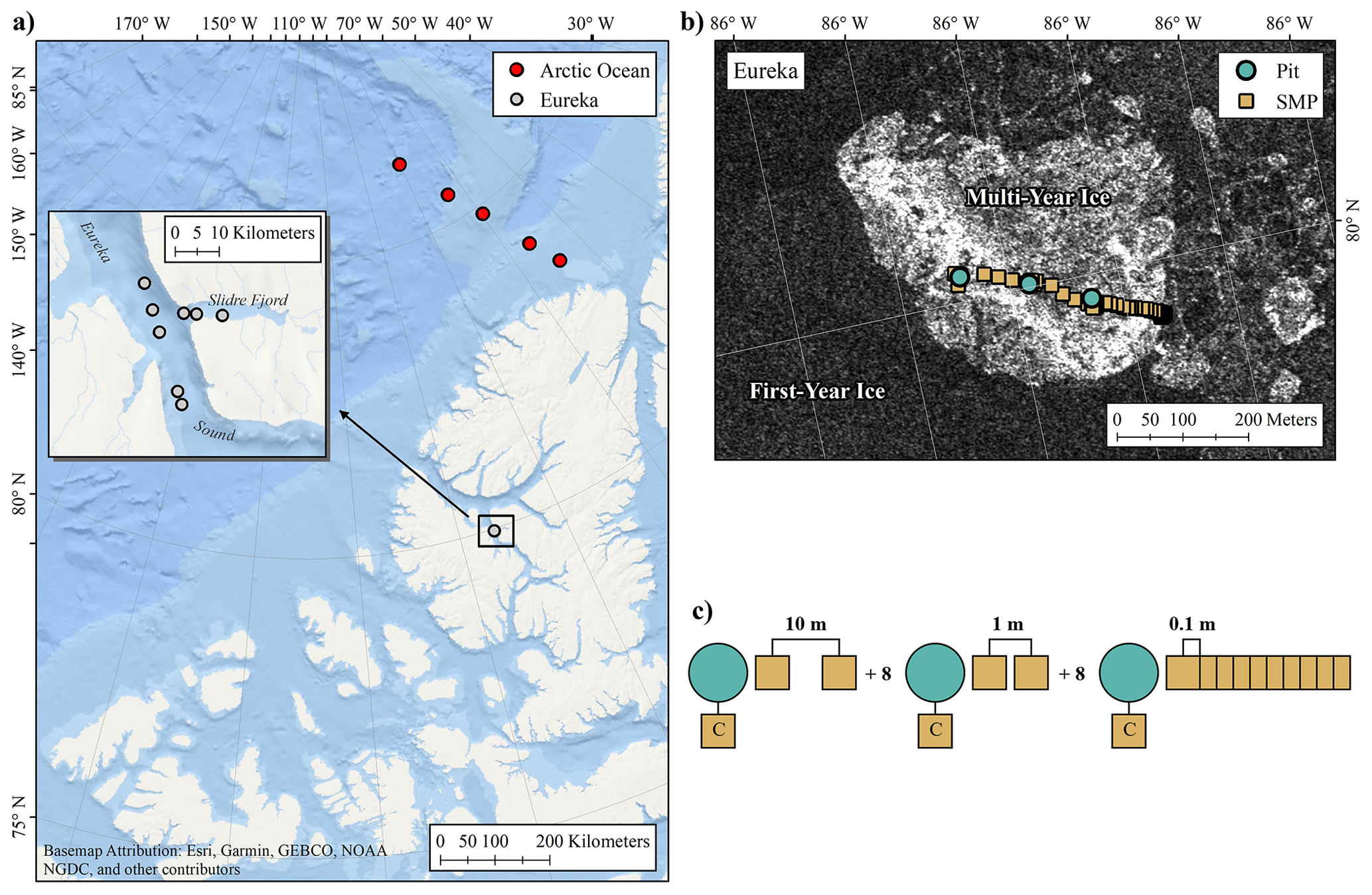
Figure 1Overview of the Eureka and Arctic Ocean (AO) snow on sea ice campaigns (a). Unidirectional SnowMicroPen (SMP) transects were collected at multiple sites to evaluate spatial variability of snowpack properties (b; Eureka MYI site shown) with sets of 10 profiles separated at distances of 0.1, 1, and 10 m, in sequence (c). Co-located SMP profiles were collected at all snow pit locations to calibrate the SMP density model of Proksch et al. (2015). Background of (b) shows RADARSAT-2 imagery near Eureka where bight returns indicate rough multi-year ice. RADARSAT-2 data and products © MacDonald, Dettwiler and Associates Ltd. (2019). All rights reserved. RADARSAT is an official trademark of the Canadian Space Agency.
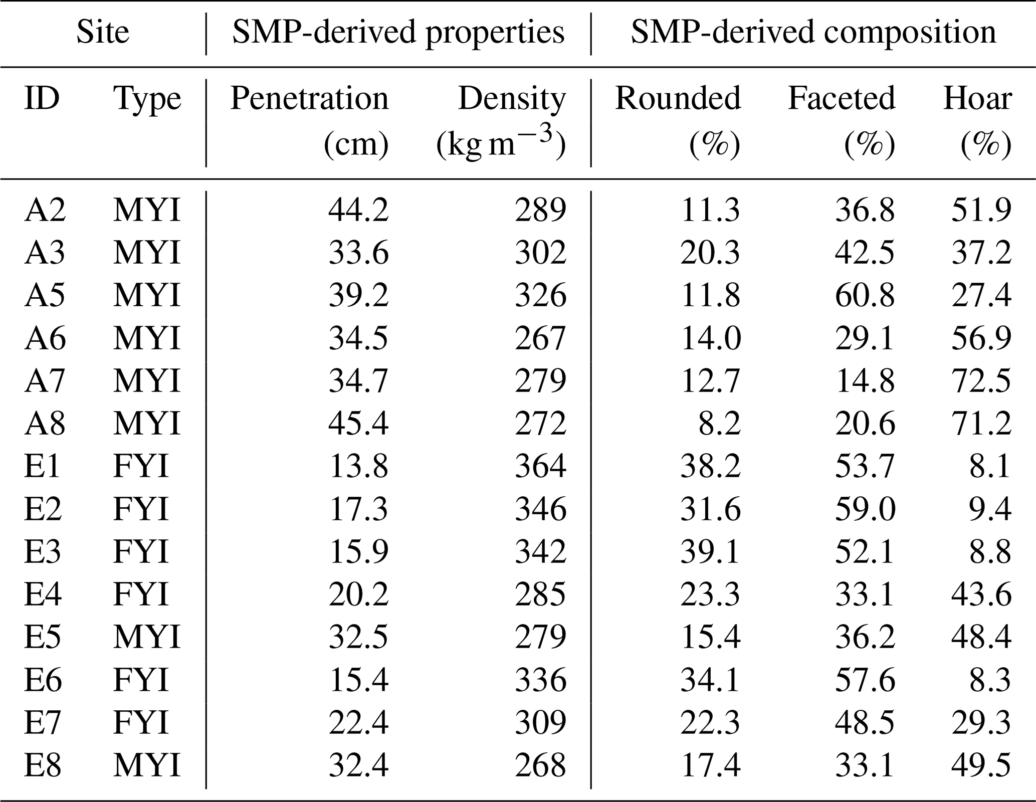
The first measurement campaign took place near Eureka, Nunavut, Canada, on landfast ice in the CAA (80.0∘ N, 85.9∘ W; Fig. 1a). Snow property measurements were collected over a 9 d period between 8 April and 17 April 2016 within Eureka Sound and Slidre Fjord. Sea ice near Eureka was principally landfast FYI with embedded floes of MYI imported from the Arctic Ocean via Nansen Sound. Similar to conditions reported in King et al. (2015), FYI near Eureka formed as large level pans with limited deformation. Imported MYI was rough in comparison and heavily hummocked from exposure to previous melt (Fig. 1b). Mean ice thickness was 2.18 ± 0.10 for FYI and 3.10 ± 0.66 for MYI evaluated near Eureka (± indicates standard deviation). Measurements at Eureka were grouped by sites (250 m × 100 m) with similar surface condition as determined from visual inspection of RADARSAT-2 imagery (Fig. 1b). At Eureka, a total of eight sites were completed with six on FYI and two on MYI (Table 1). The average distance between sites was approximately 15 km and were accessed via snowmobile from the Environment and Climate Change Canada Eureka Weather Station.
Table 1Summary of measurements completed as part of the Eureka (E) and Arctic Ocean (A) campaigns.
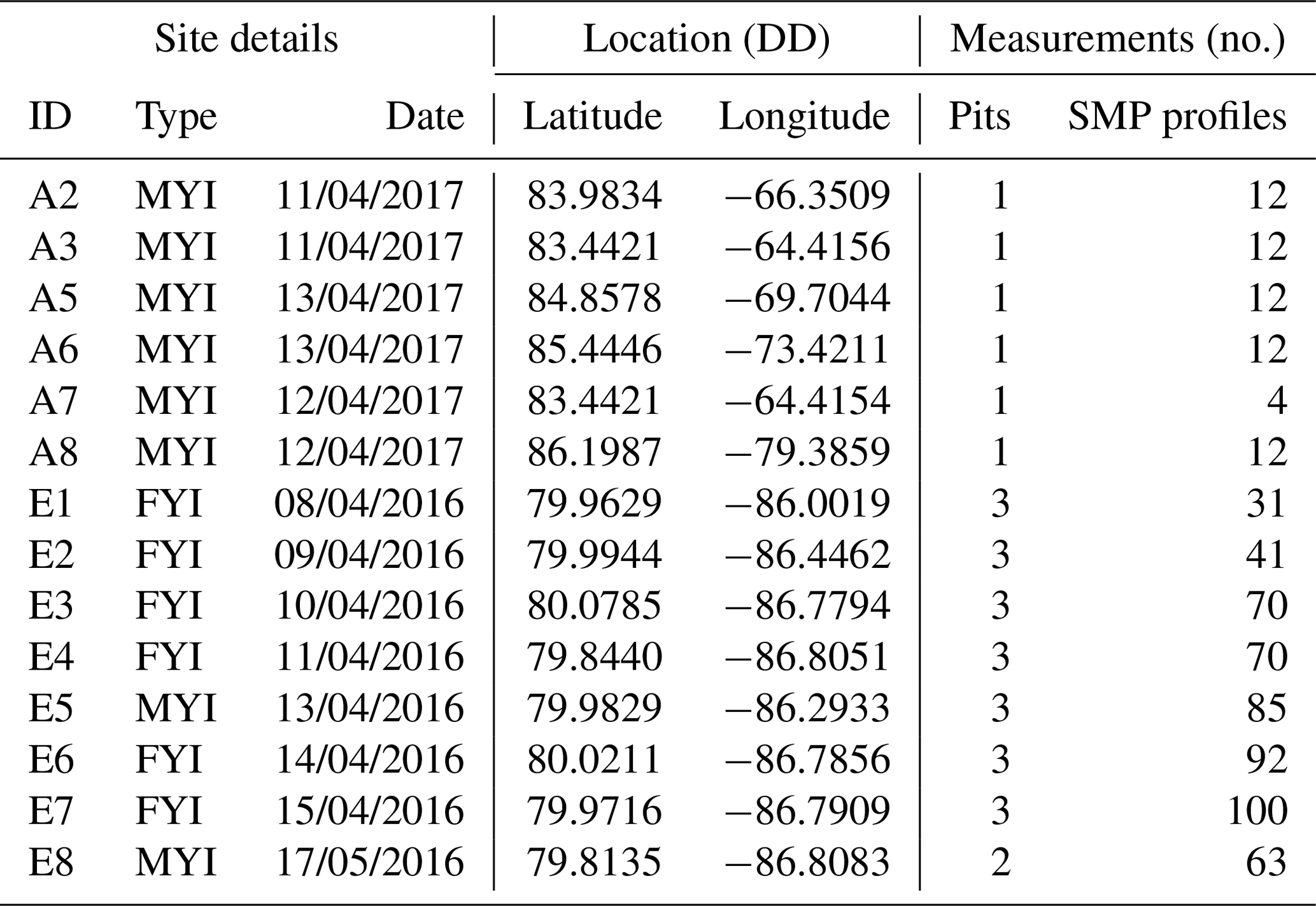
A second campaign in April 2017 focused on the characterization of MYI in the Arctic Ocean (AO; Fig. 1a). A Twin Otter aircraft was used to access sites west of the Geographic North Pole from Alert, Nunavut, Canada, along a CryoSat-2 track (see Haas et al., 2017). Measurements were carried out at six sites spanning 83.4 and 86.3∘ N between 11 and 13 April 2017 (Fig. 1a). In contrast to the Eureka campaign, the AO sites traversed an extensive region of MYI with thickness consistently greater than 3 m (Haas et al., 2017). However, with limited time at each landing site, areas characterized were much smaller than at Eureka. The average distance between sites for Alert was 175 km, spanning a large gradient of ice conditions.
2.2 Snow pit measurements
The Eureka and AO campaigns had common goals to (1) collect adjacent snow pit and SMP profiles and (2) extend characterization from single, local snow pits to larger horizontal scales using SMP transects. As such, the common core of the measurement protocol was standard snow pits used as reference. For Eureka, an average of three snow pits were excavated per site (total n = 20), and a single snow pit was completed per landing for the AO campaign (total n = 6). Once excavated, stratigraphy was interpreted via visual inspection and finger hardness tests. Heights of the interpreted layers were marked on the pit face and recorded. A 2 mm comparator card and 40× field microscope were used to classify each layer by standardized grain type as described in Fierz et al. (2009). Samples were then broadly categorized as rounded (integrating RGwp, RGxf grain types), faceted (FCso, FCsf), or depth hoar (DHcp, DHch), descriptive of predominate metamorphic processes. Trace amounts of recent snow were integrated into the rounded classification of some layers because of surface decomposition and wind-rounded grain-type mixtures (i.e. DFbk).
Snow pit density was measured as continuous vertical profiles between the air–snow and snow–ice interfaces with a 100 cm3 Taylor–LaChapelle cutter (75 g; Fig. 2a). Extracted samples were weighed in situ with a shielded A&D EJ-4100 digital scale (±0.01 g accuracy). Measurements were rejected where the cutter could not be properly filled, such as in the presence of horizontal ice features or fragile microstructure. Previous studies have shown box-style cutter measurements to agree within 9 % of high-certainty laboratory experiments (Proksch et al., 2016); however due to potential errors of omission from sample rejection, layer-specific bias may be present.
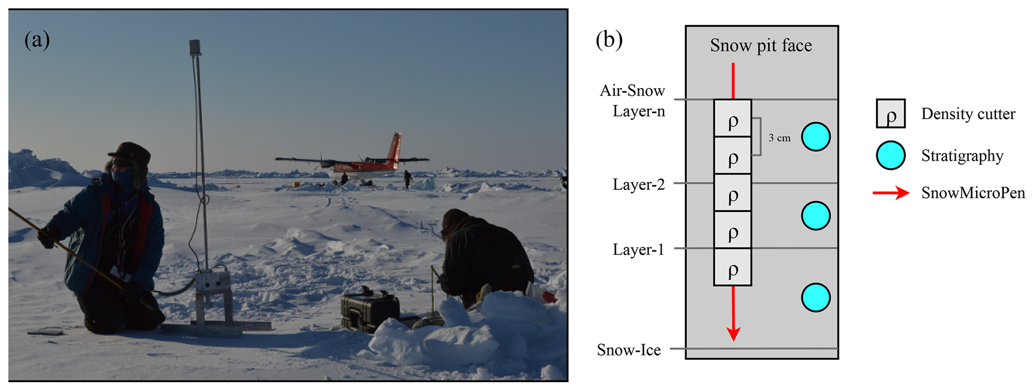
Figure 2Photo of typical SMP and snow pit measurements on MYI (a) and sketch of the sampling procedure (b). Manual density measurements (3 cm height) were collected as continuous profiles between the air–snow and snow–ice interfaces (IF). SMP profiles were compiled 10 cm behind the pit face at each site. A rigid mount was used to stabilize the SMP while penetrating hard surface slabs (a).
2.3 SnowMicroPen (SMP) measurements
A single fourth-generation SnowMicroPen (SMP) developed by Schneebeli and Johnson (1998) was used to measure profiles of penetration force (F). Operating at a constant speed of 20 mm s−1, the high-resolution force transducer of the SMP was driven vertically through the snowpack. The resulting profiles contained ∼ 250 measurements of F per millimetre, with a maximum F of 45 N and resolution of 0.01 N. Given high surface hardness, a rigid metal mount was required to stabilize the sensor and prevent rebounding on initial penetration (Fig. 2a). To preserve the penetrometer from impact with the ice surface, maximum penetration was set 1 cm shorter than the adjacent snow thickness. Coincident SMP profiles were made at 26 snow pit locations to evaluate derived estimates of snow density (Table 1). Maintaining a horizontal separation of 10 cm, profiles were located behind the snow pit wall in proximity to the manual cutter profile. After each profile, a snow depth probe was inserted into the SMP path to measure any unresolved thickness. The location of each profile was recorded with the GPS on board the SMP (±5 m accuracy).
In addition to profiles at snow pit locations, SMP transects were established to characterize spatial variability (Table 1). For Eureka, multi-scale sampling was applied where unidirectional sets of 10 profiles were separated at distances of 0.1, 1, and 10 m, in sequence (Fig. 1c). Where time permitted, additional profiles were completed with 1 m spacing adjacent to the primary transect. An average of 69 SMP profiles were collected per site near Eureka (total n = 550). It was not possible to execute an identical sampling strategy for AO sites due to time constraints. Instead, a single set of 10 profiles was spaced 1 m apart, parallel to the snow pit wall. An average of 11 profiles were made per site for the AO campaign (total n = 63).
3.1 Basis for estimation of snow density from penetrometry
The SMP force signal, F, can be linked to physical properties of the snowpack though modelling of the penetration process and related to density with an empirical model (Proksch et al., 2015). To do so, the fluctuating force signal measured by the SMP can be interpreted as the superposition of spatially uncorrelated ruptures and deflections (Marshall and Johnson, 2009). Conceptualized as a one-dimensional shot-noise process, Löwe and van Herwijnen (2012) reinterpret this relationship to compute estimates of microstructural length scale (L) without the need for a priori knowledge of snow structure. The derived quantity L represents an idealized distance between two rupturing elements of the snow structure. Proksch et al. (2015; hereafter P15), building on the work of Pielmeier (2003), relate the microstructural property L and median penetration force () to snow density through a bilinear regression:
where the coefficients (, and d) were calibrated against micro-computed tomography (uCT) in alpine, Arctic, and Antarctic environments (Table 2). Detailed methodology regarding the two-point correlation function used to compute L and other relevant parameters can be found in Löwe and van Herwijnen (2012).
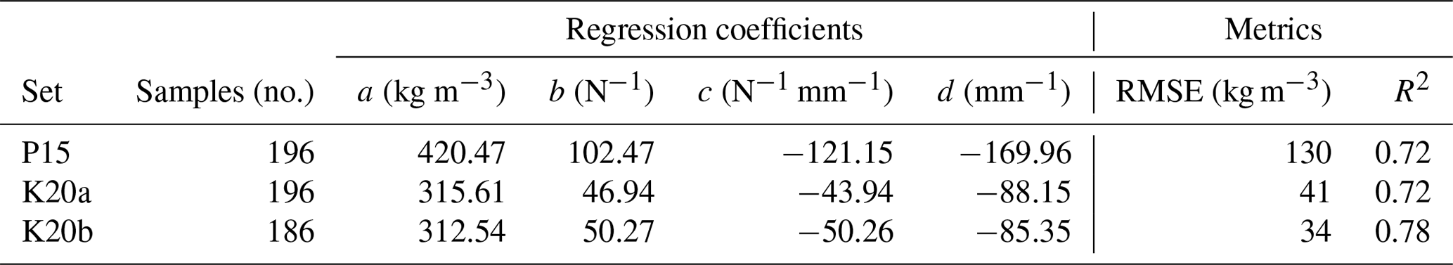
Table 2Model coefficients for Eq. (1) as originally defined in Proksch et al. (2015; P15) and recalibrated as part of this study to estimate snow density sea ice (K20).
3.2 Processing of SMP profiles for snow on sea ice
Prior to generating estimates of snow density, a series of pre-processing steps were applied to minimize SMP measurement uncertainty. First, profiles penetrating less than 90 % of the measured snow thickness were removed from analysis to minimize vertical errors of omission. Force profiles were then evaluated to isolate signal artifacts by applying a minimum noise threshold of 0.01 N following Marshall and Johnson (2009). Signals below the threshold were removed and linear interpolation was applied to infill. Once filtered, and L were computed following Löwe and van Herwijnen (2012), applying a moving window of 5 mm with 50 % overlap to meet an assumption of spatial homogeneity. Estimates of density (ρsmp) were then calculated by applying and L in Eq. (1) with an appropriate set of coefficients. The resulting data are geolocated vertical profiles of ρsmp at 2.5 mm vertical resolution.
Small-scale lateral variations in stratigraphy made validation of ρsmp challenging where the reference snow pits were physically displaced. For example, pinching or expansion of layers from variations in ice topography at sub-metre scales could lead to large differences in compared density. Adapting an approach similar to Hagenmuller and Pilloix (2016), a matching process was applied to compensate for layered differences between the target and reference snowpack. To initiate the process, first-guess estimates of ρsmp were made with the P15 coefficients for profiles at snow pit locations. Derived profiles were then divided into arbitrary 5 cm layers and scaled randomly in thickness. Individual layers were allowed to erode or dilate by up to 75 % of the original thickness, contributing towards a total permitted change of 10 % per profile. A large number of scaling permutations were generated for each SMP profile using a brute force approach (). Estimates of ρsmp were then extracted from the scaled profiles within the 3 cm height of each density cutter measurement and averaged. Best-fit alignment was selected where root-mean-square error (RMSE) was minimized between the thickness-scaled ρsmp profiles and snow pit observed density.
Figure 3 shows an example of the matching process where a basal snow feature on MYI was poorly aligned between the first-guess estimates of ρsmp and snow pit measurements. The profile was divided into 12 layers (Fig. 3a) and scaled to identify best-fit parameters for each layer (Fig. 3b). An overall stretch of 6.5 % was applied through the matching process, minimizing RMSE (54 kg m−3) and improving correlation (R = 0.83) in the example profile. Matching applied to all SMP profiles at snow pit locations resulted in a mean vertical absolute scaling of 7.4 % or 1.7 cm.
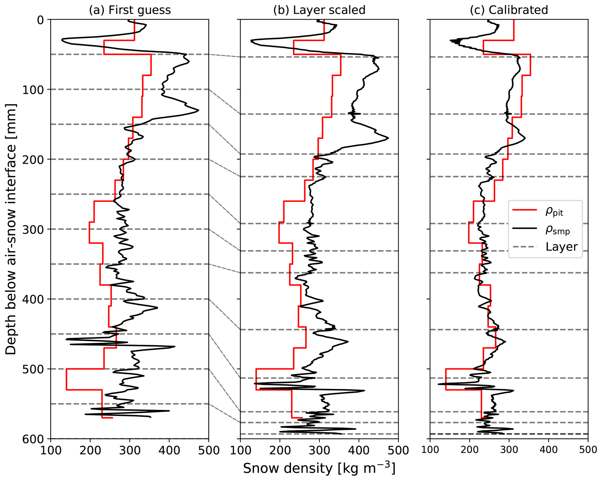
Figure 3SMP processing steps where first-guess estimates of ρsmp (a; black lines) are used to improve alignment with snow pit measurements of density (b; red lines) prior to recalibration and computation of final estimates (c). To begin alignment SMP profiles are divided into arbitrary 5 cm layers (dotted lines) and scaled randomly in thickness. Best-fit alignment is selected where RMSE between the SMP estimates and snow pit measurements are minimized. The matching process accounts for differences in the target snowpack due to the 10 cm separation between profiles. The example shown is for Eureka site 5 on MYI.
3.3 Calibration of the SMP snow density model on sea ice
Once aligned, estimates of ρsmp were compared against in situ snow pit densities to quantify retrieval skill. An evaluation of the P15 parameterized density model is shown in Fig. 4, including measurements from all 26 snow pit locations (n = 196). Estimates of ρsmp were biased high relative to the snow pit reference with a large RMSE of 124 kg m−3 (Table 2). The observed bias increased with density, leading to unrealistic overestimates for wind-slab-classified samples (165 kg m−3 RMSE). Conversely, errors were lowest for low-density depth hoar (96 kg m−3 RMSE). Comparing estimates from the two campaigns, Eureka had a higher RMSE (135 kg m−3) than measurements at AO sites (98 kg m−3), but the discrepancy was related to lower overall density reported on MYI rather than campaign-specific bias.
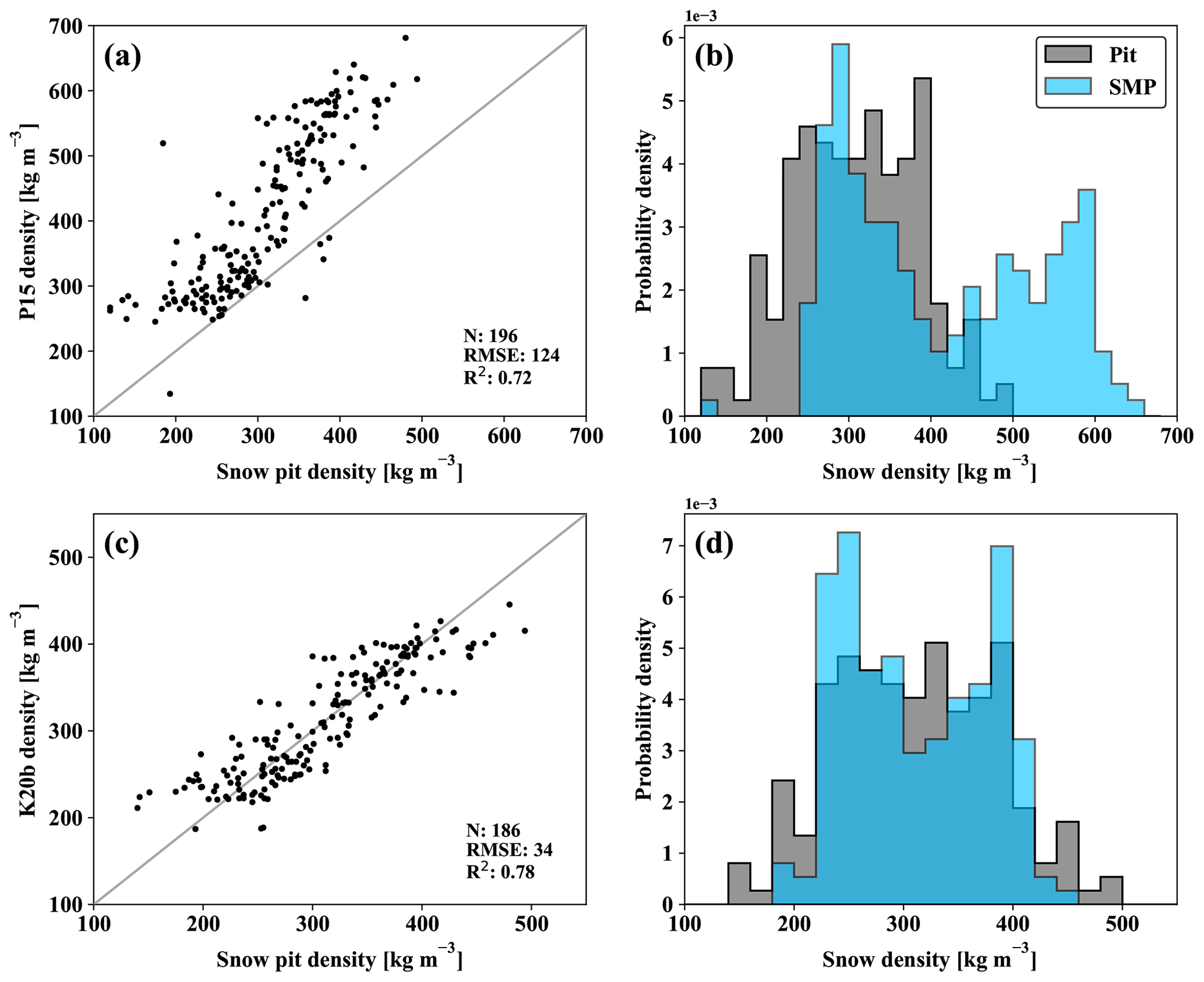
Figure 4Evaluation of the original SMP density model of Proksch et al. (2015) (P15; a) and recalibrated coefficients for snow on sea ice (K20b; b). Retrieved distributions are shown for the P15 (b) and K20b (d) parameterizations of Eq. (1) with a common bin size of 20 kg m−3. In all cases, the reference measurements are manual density cutter measurements of snow density.
Despite a 41 % RMSE, the P15 parameterized estimates of ρsmp were well correlated with snow pit measurements (R2= 0.72; p<0.01; Table 2). An ordinary least-squares (OLS) regression was used to recalibrate P15 where snow pit measurements were available as reference. Values of and L identified in best-fit scaling of the SMP profiles were used in the regression, along with the corresponding density cutter measurements. A 10-fold cross-validation was applied where inputs were divided into roughly equal groups and used to train the regression with all but a single fold which was reserved for testing. Test-train permutations were iterated until each fold had been used independently in testing to minimize sampling bias. Coefficients were averaged across fold combinations and reported with RMSE and R2 in Table 2.
Calibrated with the snow pit densities, retrieved coefficients of the regression differed substantially from P15 but remained identical in R2 (Table 2). Applying the revised coefficients (referred to as K20a), RMSE was reduced to 41 kg m−3 or 13 % of the observed mean. Previously observed P15 bias was also minimized with no significant trend in residuals (0.1 kg m−3). Given that the profiles used to evaluate model skill were physically displaced, it was unlikely that all matched comparisons were strong candidates for the recalibration. As such, a revised set of coefficients was prepared where outliers defined as the 95th percentile of absolute error in the initial comparison were removed from the regression (>85 kg m−3; n = 10). Data associated with these outliers were few in number and primarily associated with layer boundaries on FYI. Regression of the constrained input (K20b; Fig. 4b) showed small differences in the retrieved coefficients (Table 2) along with improved skill (R2=0.78; 34 kg m−3).
To evaluate dependency of the regression parameters, their respective relationships with observed snow density are shown in Fig. 5. Median force (), once log-transformed, was well correlated with density in the combined ice surface and campaign dataset (R = 0.76; Fig. 1a). However, the observed relationship with weakened for samples collected on MYI (0.69 R), in particular those as part of the Eureka campaign (R = 0.46). In contrast, the microstructural parameter L remained well correlated with density regardless of ice type or campaign (; Fig. 1b). In all coefficient parameterizations (P15 and K20) the dependent variables and interaction term were found to be significant in the OLS regression. Although some dependency on snow conditions with respect to ice type was apparent, the K20b parametrization was applied globally as the relationship was unlikely to be driven by ice type but rather as some function of ice surface roughness which was unaccounted for in this study.
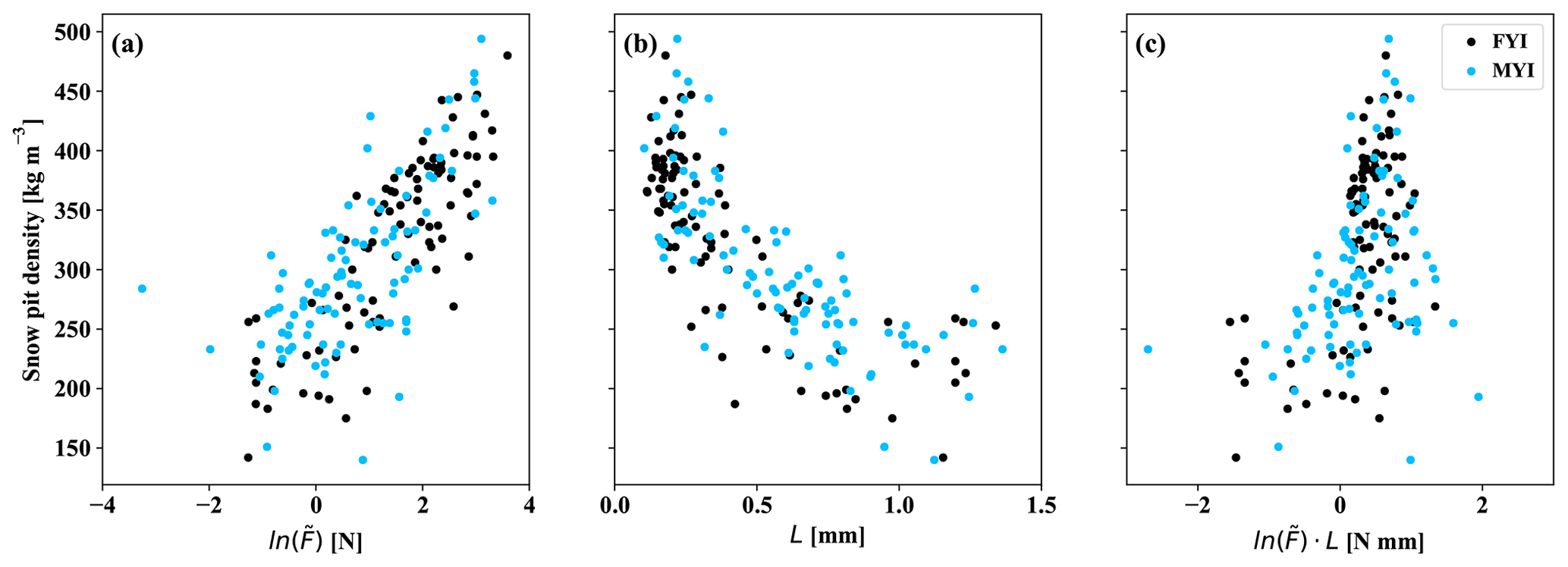
Figure 5Comparison of the SMP regression parameters and corresponding snow pit observed density. Parameters include log-transformed median force (), (a), microstructure length scale (L, b), and an interaction term (, (c). Relationships are separated by ice type (FYI and MYI).
3.4 Classification of SMP density profiles by layer type
To quantify the stratigraphic variability of snow density, a support vector machine (SVM) was implemented to partition the SMP density profiles by layer type (Cortes and Vapnik, 1995). SVMs apply hyperplanes in high-dimensional space to separate classes by maximizing distance from support vectors (i.e. a hyperplane which best delineates the nearest data pairs between classes). Automated learning methods have previously been applied to support classification of SMP profiles (e.g. Havens et al., 2013) and are well suited to rapidly process the available transect data. Learning methods for SVM classification were adapted from scikit-learn (Pedregosa et al., 2011) and trained on snow pit (layer type) and SMP () information extracted according the Sect. 3.2 procedures. Applying a linear kernel, the classifier was 10-fold cross-validated similar to the OLS regression; however, sampling was stratified to ensure a minimum of 10 samples per layer-type class in each fold. Classified estimates from each profile were smoothed with a median window to remove thin layers with thickness less than 1 cm (window size = 5). Cross-validated results of the SVM classifier are presented in Table 3 as a confusion matrix. Accuracy, defined as the percentage of true positive or true negative predictions, was 76 % overall when compared against the snow pit reference samples. Layer-type-specific accuracy was comparable for rounded and faceted types (76 %) and improved for depth hoar (82 %). Misclassification errors were highest for rounded types, where samples were most often confused for faceted types (24 %).
Table 3Normalized confusion matrix for the support vector machine (SVM) layer-type classification of SMP profiles compared against known snow pit samples. Results were 10-fold cross-validated and samples were stratified to ensure a minimum of 10 samples per layer-type class in each fold.
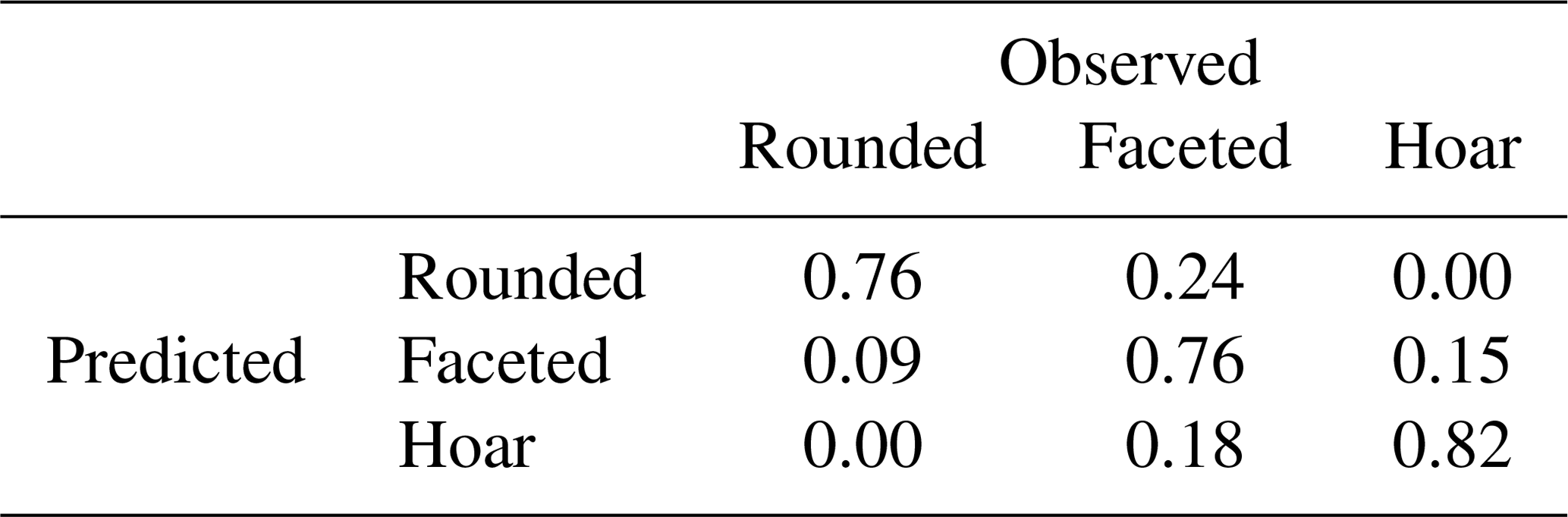
Figure 6 shows an example of a classified SMP profile compared against snow pit observed stratigraphy on MYI near Eureka. Trained against a generalized layer-type classification scheme, the methodology is incapable of identifying inter-layer variations apparent in the manual snow pit observations. However, by identifying major transitions, the classified profile can be used to quantify differences in layered composition observed across both ice type and campaign. Moreover, by counting the number of transitions between layer-type classifications, an approximate count of snowpack layers can be made.
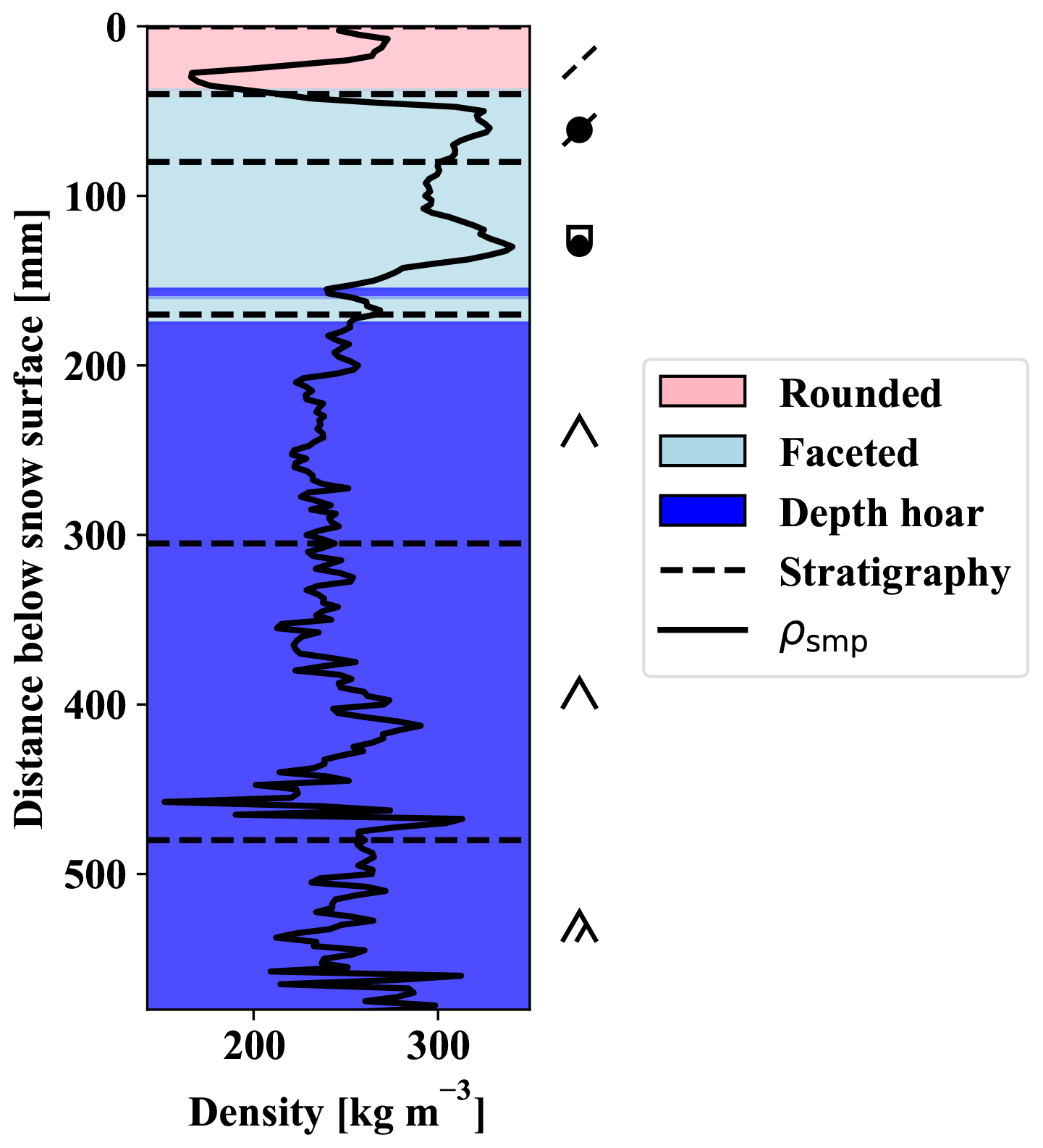
Figure 6Automated layer-type classification of a SMP profile collected on sea ice where colours indicate classification result. Horizontal dashed lines indicate heights of snow pit observed stratigraphic layers at the same location. Snow layer classification follows standardized colours and symbols described in Fierz et al. (2009).
4.1 Snow pits
Central to the density model evaluation was the acquisition of a limited number of high-certainty snow pits (n = 26). Each served as a density reference for the SMP calibration but also provided baseline information on stratigraphy to frame the transect analysis. By the April timing of the campaigns, evidence of wind redistribution and temperature gradient metamorphism was widespread, characteristic of late-winter Arctic snowpack. Mean thicknesses of the snow pits were 20.8 ± 6.1 and 38.0 ± 12.7 cm for FYI and MYI, respectively. Stratigraphic complexity was apparent on MYI where seven layers were present on average as opposed to four on FYI. Bulk density of snow pits on FYI (320 ± 33 kg m−3) was higher in comparison to MYI (300 ± 36 kg m−3), a function of limited variation in ice surface topography on the level FYI near Eureka.
Consistently across snow pits, density was highest in proximity to the air–snow interface where rounded grain types were prevalent. Commonly known as wind slab, these layers were a product of mechanical wind rounding and subsequent sintering. Corresponding grain classifications were mainly wind-packed (RGwp) or faceted rounded (RGxf) types. Density of the wind slabs was comparable between ice environments and campaigns with an average of 375 ± 49 kg m−3 (Table 4). Lower-density slab features occurred where wind-broken precipitation (DFbk) was inter-mixed with the smaller mechanically rounded grains. For example, at Alert sites 6 and 8, ∼ 3 cm of decomposing precipitation was present at the air–snow interface, leading to lower surface densities (∼ 222 kg m−3). In general, these so-called soft slab features were more common on MYI where rough ice features buffered windblown snow efficiently.
Table 4Mean density cutter measurements from snow pits separated by layer type and campaign.
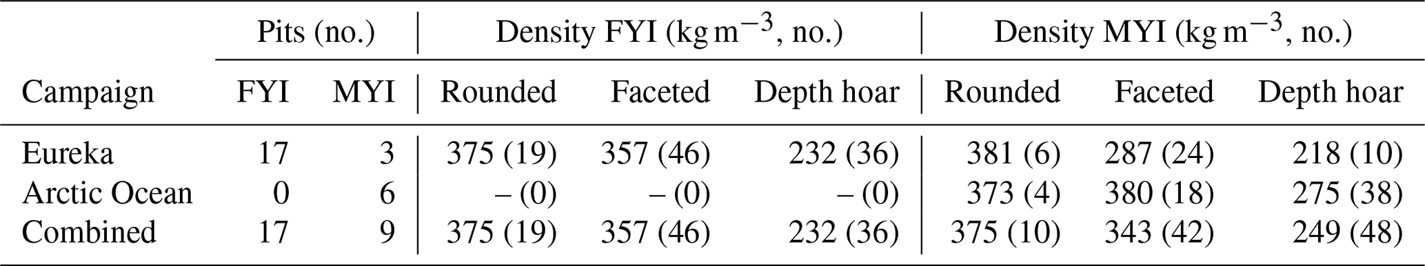
Layers below the surface slab were similar in appearance, but inspection of the grains revealed tightly packed facets. Distinct in microstructure, these former wind slabs showed clear signs of kinetic growth while maintaining a well-bonded structure. Density of the mid-pack faceted layers was comparable to the surface features for the AO campaign (380 kg m−3) but was slightly lower for Eureka (287 kg m−3). At the base of the snowpack were multiple layers of large diameter depth hoar, texturally distinct from the overlying slab and faceted layers. Microstructure of the depth hoar was characterized by weakly bonded cups (DHcp) at times clustered as large chained units (DHch). The unconsolidated structure of the depth hoar was fragile, often collapsing when inspected by touch or tool. Density of the depth hoar layer was consistently lowest, with a small range of observed variability (Table 4).
4.2 SMP profiles
Despite layered similarity, it was difficult from snow pits alone to directly compare proportional composition or determine process scales over which structural correlations might persist. The SMP transects presented a unique opportunity to extend analysis beyond the point scale and link layers between snow pits by drastically increasing the number and spatial diversity of profiles. Once processed, the SMP profiles collected on sea ice provided 58 882 estimates of snow density, representing approximately 147 m of vertical variation. Each profile also contained estimates of proportional composition by layer type through automated classification, facilitating layer density comparisons and spatial analysis.
Figure 7 shows the aggregated results of the SMP transect profiles where snow density measurements were separated by ice surface and layer type. Separated by ice type (FYI and MYI), bulk densities (vertically integrated) are represented in two overlapping but distinct distributions (Fig. 7a). Profiles collected on FYI, and therefore exclusively near Eureka, formed a slightly left-skewed distribution with mean density of 327 ± 42 kg m−3 (n = 402). In contrast, densities on MYI were right-skewed with a mean of 277 ± 30 kg m−3 (n = 211). Separating the MYI profiles by campaign shows small differences between Eureka (272 ± 27 kg m−3, n = 148) and the AO (290 ± 31 kg m−3, n = 63). However, these differences were small in comparison to the larger shift between MYI and FYI. Overall, the opposing skew shows a clear shift in snow density by ice surface type for the observed domains independent of campaign.
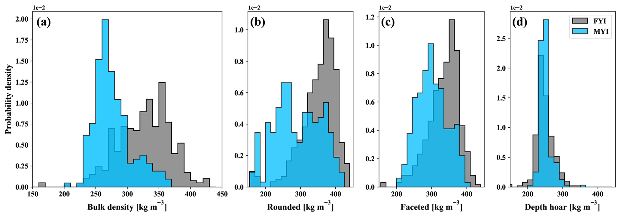
Figure 7Bulk density (vertically integrated) derived from SMP profiles on first-year (FYI, n = 402) and multi-year (MYI, n = 211) sea ice (a). Automated profile classification was used to separate the high-vertical-resolution (2.5 mm) estimates of snow density and produce layer-type distributions for rounded (b), faceted (c), and depth hoar (d) classes.
Given that all profiles were classified by layer type (see Sect. 3.3), it was also possible to evaluate distributions of density separately for rounded, faceted, and depth hoar features (Fig. 8; Table 5). Composition of the thin Eureka FYI snowpack (18.1 ± 8.8 cm) was primarily faceted, represented by 50.0 ± 18.1 % of total thickness on average. Measurements classified as faceted had on average a density of 336 ± 43 kg m−3, forming a left-skewed distribution (Fig. 8). Rounded layers in proximity to the air–snow interface were thinner, accounting for 30.2 ± 15.0 % of total thickness (Fig. 8), with a mean density of 352 ± 51 kg m−3, also represented in a left-skewed distribution (Fig. 7b). At the base of the snowpack on FYI, depth hoar was the smallest fractional component (19.8 ± 18.4 %; Fig. 8) and had the lowest mean density (248 ± 27 kg m−3; Fig. 7d).
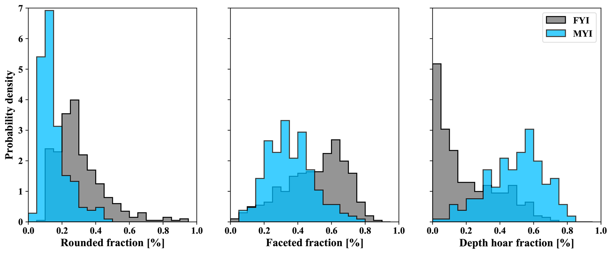
Figure 8Fractional snowpack composition by rounded, faceted, and depth hoar layers from the SMP profiles on first-year (FYI) and multi-year (MYI) sea ice. Classification methods for the SMP are described in Sect. 3.4.
Table 5Snow density and layering derived from SMP profiles at each field campaign site using Eq. (1) and the automated classification procedures described in Sect. 3.4.
Composition on MYI shifted towards a larger proportion of depth hoar (49.2 ± 16.3 %) within the overall thicker snowpack (34.7 ± 16.8 cm). Density of the depth hoar on MYI was comparable to FYI with means of 247 ± 15 and 257 ± 18 kg m−3 for the Eureka and AO sites, respectively. Mid-pack faceted layers were well represented at 35.5 ± 13.7 %, albeit with lower density overall at 301 ± 43 kg m−3 and notable decreases at Eureka (294 ± 41 kg m−3). Layers classified as rounded composed the remainder of the volume at 15.3 ± 8.5 %. The density distribution of rounded layers on MYI was bimodal (Fig. 7), corresponding with the presence of decomposing precipitation in mixed-type layers. Mean density of rounded layers on MYI was on average 291 ± 65 kg m−3 with slightly higher densities observed at AO sites (306 ± 67 kg m−3) over Eureka (285 ± 63 kg m−3).
As a proxy for the number of observed layers, transitions between layer-type classifications were summed for each profile. Figure 9 shows probability densities associated with layer-type transitions separated by ice type. As in the snow pits, stratigraphic complexity was greater on MYI with an average of 6.9 layer-type transitions as opposed to 4.5 for FYI. Of the transitions, those associated with faceted layers on MYI were most prevalent with an average of 2.9 per profile. Faceted transitions on FYI were fewer in number at 1.9 on average. Depth hoar layers were 2.8 on average for MYI and 1.5 for FYI. Finally, in both environments the average number of rounded transitions was 1.1 with no more than 3 transitions identified in any profile.
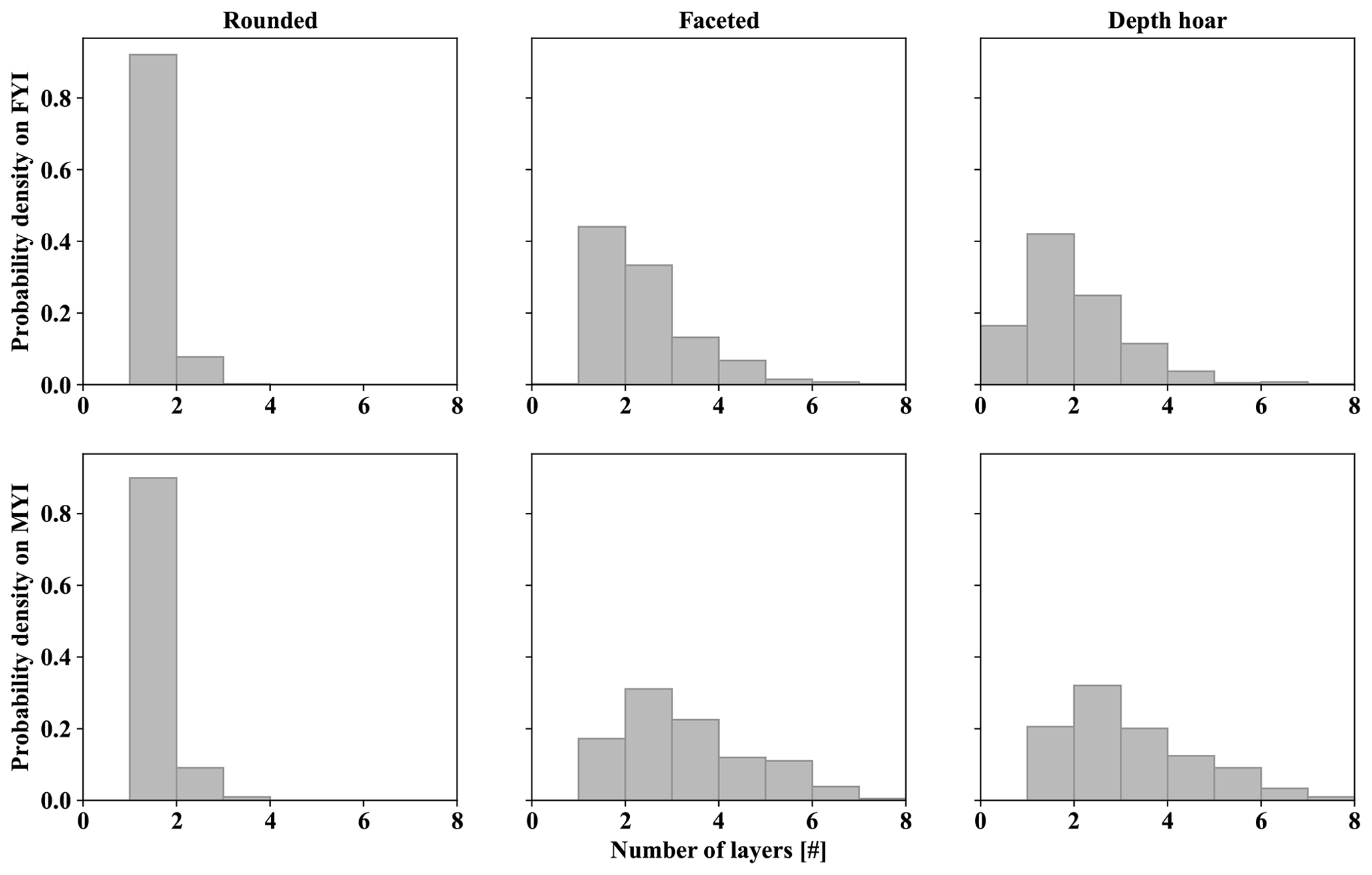
Figure 9Distribution of the number of snowpack layers as derived from the SMP transect profiles. Transitions between layer types from the automated SMP profile classifications are used as a proxy for traditional snow pit layer counts.
4.3 Length scales of variability
Large standard deviation relative to most layer-type fractions indicated strong stratigraphic variability within the SMP transect dataset. Given that these variations are driven at local scales by ice topography and weather (wind and precipitation), it can be expected that structural similarities persist at some process scale. To evaluate differences in length scale, estimates of spatial auto-correlation for layer-type composition were computed using Moran's I (Moran, 1950):
where x represents rounded, faceted, or depth hoar volume fractions at locations i and j displaced at a lag distance of d. Equation (2) was evaluated for pairs of profiles separated by d from 1 to 100 m in 1 m increments for each layer type. To compensate for geolocation errors, a tolerance of ±5 m was applied to d, corresponding with GPS accuracy of the SMP. Weighting (w) of Eq. (2) takes on a value of 1 when pairs were displaced at d±5 m and 0 otherwise. On average, 412 pairs were evaluated per lag of d on FYI and 333 on MYI. The resulting spatial auto-correlation analysis of snowpack fractional composition is presented in Fig. 10. At scales beyond 100 m the number of profile pairs was limited given the ∼ 250 m length of each site and is therefore not presented.
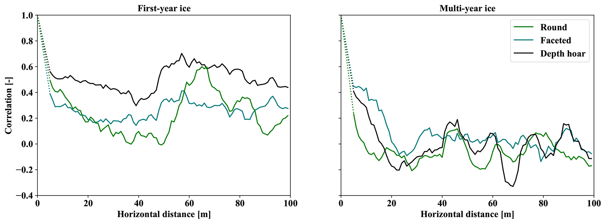
Figure 10Spatial auto-correlation of snowpack fractional composition by layer type on FYI and MYI as estimated from classified SMP profiles. Dotted lines show assumed correlation at length scales less than 1 m where geolocation uncertainty of the profiles precludes analysis.
On FYI, all layer types showed similar trending in auto-correlation with distinct minimums spaced at approximately 40 m (Fig. 10). After an initial decline, depth hoar fraction on FYI remained moderately correlated at scales of 100 m and was also the strongest of the layer-type correlations (R = 0.70 at 52 m). While the magnitude of the remaining rounded and faceted fraction layer-type correlations was lower, spatial trends on FYI were highly correlated with each other. In contrast, correlations dropped quickly on MYI for all layer types and remain low at scales of 100 m (Fig. 10). Faceted-type layer fraction maintained spatial correlation for the longest period on MYI but reached 0 at only 16 m. The result suggests spatial persistence of layered features on FYI beyond the available data. In contrast, strong variations in snow structure on MYI at short scales indicate the presence of distinct drivers and variability absent on the level FYI near Eureka.
In the context of radar altimetry and sea ice freeboard retrievals, errors related to snow density can be described as a propagation bias where speed of the interacting wave is reduced in snow (Kwok et al., 2011). Without accounting for this reduction, radar-measured distance to a scattering horizon may be overestimated, or in a retrieval, the height of the sea ice freeboard may be underestimated if the primary scattering horizon is assumed to be the ice surface. Established empirical relationships with permittivity (i.e. Ulaby et al., 1986) can be leveraged to quantify reductions in wave speed (cs):
where ρs is observed or modelled snow density. Estimates of path length difference (δp) relative to propagation in free space can then be computed with respect to variations in snow thickness (hs) as in Tilling at al. (2016):
Utilizing these equations, differences in propagation bias were evaluated for two scenarios where snow density was (1) determined from climatology and (2) parameterized from SMP measurements. The first configuration mirrors common practice in radar altimetry where the two-dimensional quadratic of Warren et al. (1999) was used to compute bulk density based on location and month. The second configuration leverages the high vertical resolution of the SMP profiles to approximate variations in wave propagation at the millimetre scale. One-way path length difference from the SMP () was calculated as the summation of δp for each 2.5 mm vertical estimate. In both scenarios, height of the snowpack (hs) was defined as SMP total penetration and δp was evaluated at each profile location.
Given the small geographic extent of the Eureka campaign, climatological estimates of snow density predicted no spatial variability with a mean of 298 kg m−3. This was unsurprising given that the Warren et al. (1999) estimates are generally considered invalid within the CAA due to a lack of observations in the region. As such, a static value of 300 kg m−3 was applied, representative of a typical parametrization used in altimetry studies (e.g. Tilling et al., 2016). For AO sites, climatological estimates fell within a narrow range between 317 and 321 kg m−3, across a nearly 3∘ difference in latitude. From climatology, the average reduction in wave speed relative to free space () was estimated to be 0.809 for Eureka and 0.799 for AO sites. With little variability in density, δp was driven strongly by snow thickness, where longer physical paths lead to larger delays (Fig. 11a). As a result, predicted bias was greatest on MYI north of Alert (9.2 cm), despite slower expected propagation within the higher-density Eureka snowpack.
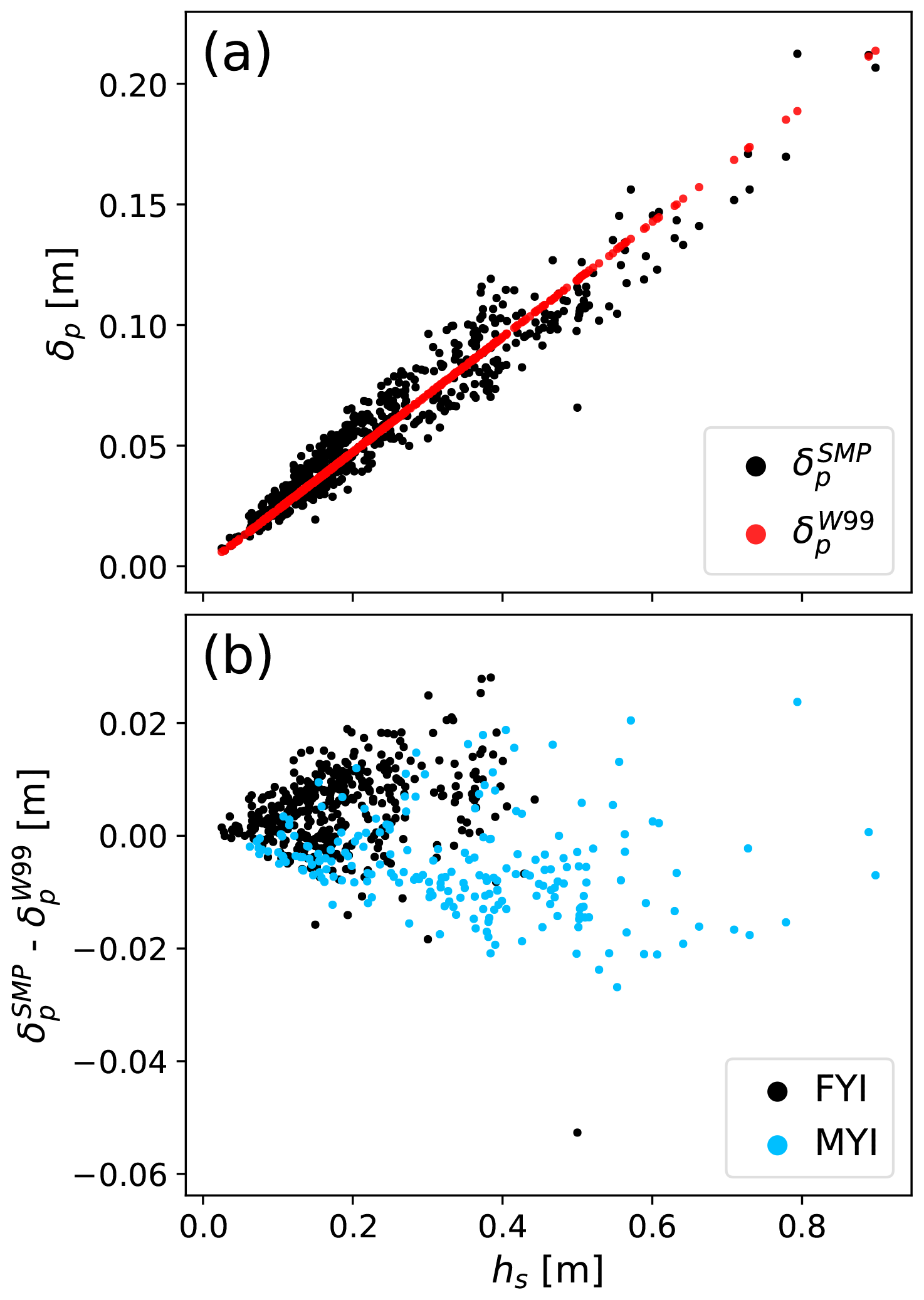
Figure 11Changes in estimated radar propagation bias (δp), (a) relative to snow thickness (hs) based on density estimated from climatology () and measured from SMP profiles (). The two sets of estimates were subtracted to show potential errors associated with the use of climatology over known snow densities (b).
For the second scenario, average wave speeds relative to free space remained similar for Eureka (0.803) but were increased for AO profiles (0.815). Estimates of propagation bias computed with an explicit representation of density () showed limited sensitivity to the observed variations (Fig. 11a). At hs corresponding with the Eureka FYI mean (18.2 ± 1 cm), the spread in was approximately 2.3 cm with an average propagation bias of 4.7 cm. Conversely, for AO sites (39.7 ± 1 cm) the spread in increased to 3.8 cm with a mean propagation bias of 9.3 cm. To quantify errors related to the use of climatology over in situ observations, the two scenarios were differenced (; Fig. 11b). Assuming as truth, potential errors on FYI ranged from −4.0 to 2.6 cm with a mean of 0.5 ± 0.6 cm. On MYI, where densities were generally lower, the mean difference was −0.5 ± 0.8 cm, spanning a small range of −2.5 to 2.3 cm. Errors on MYI between the AO and Eureka campaigns were in close agreement with means of −0.5 ± 0.7 and −0.2 ± 0.9 cm, respectively.
Considerable skill was demonstrated in SMP retrievals of snow density by Proksch et al. (2015) but there had been no previous application on sea ice or in environments with a comparable snowpack dominated by wind slab and depth hoar. Evaluation of the P15 coefficients at 26 snow pits on sea ice showed a strong positive bias in SMP-derived density compared to manual density cutter measurements. As a technical limitation, Proksch et al. (2015) noted that future hardware revision of the SMP would necessitate recalibration due to differences in signal digitization. The P15 results appear to confirm this limitation which was addressed with an OLS regression of the coincident density cutter measurements and SMP profiles. The recalibrated coefficients showed errors 10.9 % of the observed mean when evaluated across a selected set of reference measurements (34 kg m−3, n = 185). This was comparable to the P15 reported error (10.6 %) and within the range of the reported skill (R2=0.64–0.80). Differences in error between ice environments and campaigns were nominal (< 4 kg m−3), demonstrating confidence in the application of a globally optimized set of coefficients.
Observed errors in the snow density may be accounted for by limitations in the snow pit and SMP procedures. First, density cutter measurements used as reference, as opposed to high-certainty micro-CT, include baseline errors of up to 8 % (Proksch et al., 2016). Sampling in depth hoar was a particular challenge where insertion of the cutter led to collapse of the fragile microstructure. Evaluation of depth hoar was further complicated by low signal-to-noise ratio where weakly bonded grains produced little variation in the SMP-measured force. As a result, errors associated with depth hoar (14.0 %) were greater than rounded (10.7 %) or faceted (8.6 %) layers. Errors associated with the higher-density slab features may also be present due to unaccounted interactions between failing elements in the penetration model (Löwe and van Herwijnen, 2012). Representing two extremes, wind slab and depth hoar presented challenging retrieval scenarios; however the errors appear consistent with those expected from manual density cutter measurement and previous study.
Differences between the two ice type environments (MYI and FYI) showed median force (F) to be an unreliable predictor of snow density, particularly on MYI (Fig. 5). This was consistent with Marshall and Johnson (2009), who first identified environment-specific sensitivity of the SMP force, leading Proksch et al. (2015) to include the microstructural term L in the empirical model. The relationship between L and snow density was found to be independent of ice environment or campaign, acting to balance the retrieved density where signal-to-noise ratio was poor. Limiting the regression inputs in Sect. 3.3 to profiles collected only on MYI shows the strong influence of L where retrieved coefficients place increased weight on microstructure (+42 %). The observed dependencies were unlikely to be driven by ice type but rather by associated differences in ice topography and therefore retained snow structure. Differences in snow structure were clear between the two ice environments; however quantitative evaluation of how ice topography might be used to further refine coefficients in Eq. (1) was beyond the scope of this work and will require measurements in deformed FYI environments.
An average bulk density of 310 ± 37 kg m−3 was measured across all profiles included in this study (n = 615). Separated by ice type, contrasting distributions were presented where density on the windswept FYI was typically greater (Fig. 7a). Despite separation by a full year, and hundreds of kilometres, the MYI measurements from the AO and Eureka sites were similar in bulk density at 289 and 272 kg m−3, respectively. Evaluation of the snowpack structure showed depth hoar composition to be a driver of reduced density on MYI relative to FYI. At the local scales, melt ponds and hummocks on MYI serve to trap larger amounts of snow earlier in the season (Radionov et al., 1996; Sturm et al., 2002). Coupled with strong temperature gradients, favourable conditions for the development of a substantial depth hoar layer were common to most MYI sites. Ice topography control on the internal structure of the snowpack, and ultimately bulk density, was also apparent in the length scale analysis (Fig. 10). Rapid decorrelation of layered structure on MYI suggested that the hypothesized ice topography interactions occurred on relatively short length scales, driving high spatial variability particularly in depth hoar. In contrast, where large smooth floes were typical for Eureka, covariance of the layer composition on FYI persisted over large distances (> 100 m). The observed variations showed a periodicity common to length scales associated with snow dunes or interactions between drifted elements (Sturm et al., 2002; Moon et al., 2019). In the future it would be instructive to evaluate how information on surface roughness can be used to constrain understanding of internal snowpack structure between ice type environments where clear contrast exists.
A limited number of studies were available to place the observed stratigraphy in the context of other Arctic regions. Measurements collected during N-ICE2015 (Merkouriadi et al., 2017) in the Atlantic sector of the Arctic Ocean described a predominantly faceted composition on FYI (48 %) and second-year ice (54 %). Although the data presented in this study contain no second-year ice, the FYI faceted composition is in agreement, as are bulk densities in the relatively flat and windswept environments. Faceted layers observed in both campaigns originated as surface slabs, buried by successive winter storms. With density and hardness comparable to the overlying wind slab, the differentiating factor in evolution was length of exposure to strong temperature gradients (Derksen et al., 2009; Domine et al., 2012). Snow pits consistently had measured temperature gradients sufficient for kinetic grain growth on FYI (25.7 C m−1 on average; Colbeck 1983). While these layers had not fully converted to depth hoar due to high initial density (Akitaya, 1974), the larger faceted crystals were texturally distinct, separating the wind slab from depth hoar. Improved understanding of how these faceted layers evolve at larger scales may be important in remote sensing or thermodynamic applications as they contribute enhanced scattering and reduced thermal conductivity relative to their wind slab origin types.
Snow stratigraphy reported during SHEBA in the Beaufort Sea (Sturm et al., 2002) showed greater wind slab composition overall (42 %), although this varied considerably with ice surface roughness. Analysis during SHEBA suggested that increased wind slab fraction was associated with smoother ice classes and therefore thinner snowpack. Similar observations inferred from the SMP profiles showed fractional composition by wind slab to increase by 46 % on FYI over MYI because surface roughness conditions were much smoother. At small scales, portions of slab and hoar approached parity during SHEBA where precipitation was intercepted earlier and retained within hummocks. Consolidating the wind slab and faceted layer classifications on MYI, the SMP-derived composition was also roughly equal when compared to depth hoar (52 % for AO and 51 % for Eureka). In the case of both N-ICE2015 and SHEBA, direct comparison of the snowpack composition is difficult due to different measurement protocols, but common themes regarding the influence of ice topography on snowpack stratigraphy were clear.
Applying the SMP measurements to compute differences in radar propagation showed small differences compared to the use of climatological density. In comparison to the Warren et al. (1999) climatology, density on MYI in the AO was approximately 10 % lower, insufficient to drive strong uncertainty in radar-derived freeboard. Amongst the SMP-derived parameters, penetration bias most greatly influenced fractional composition by rounded-type layers (R = −0.73) on both FYI and MYI. High surface densities resulted in wave speeds 3 % slower than the remaining snowpack, having the most significant impact with respect to increased proportion. However, the overwhelming influence on the propagation bias in this study remains snowpack thickness (R = 0.97).
Although the result regarding density uncertainty in radar altimetry suggests that use of constants to represent density may be sufficient, several issues persist that should be addressed prior to making a conclusion. First, the work of Nandan et al. (2017) demonstrated that penetration is negatively impacted by the presence of brine within the snow volume on FYI. In Sect. 5, the role of salinity was not addressed for profiles on FYI and is likely to be a much larger and inverse uncertainty. Second, snow conditions evaluated in this study were dry and thus do not consider variations in scattering horizon that can be attributed to temperature or wetness (Willatt et al., 2011). Finally, in addition to density, Proksch et al. (2015) demonstrated the ability to retrieve snow microstructural properties from SMP signals. Lacking a reference for calibration, microstructural quantities were not evaluated as part of this study but in the future could be used to address waveform uncertainty corrected in some products (Ricker et al., 2014).
The recent shift towards younger Arctic sea ice (Maslanik et al., 2011) along with increased winter precipitation (Zhang et al., 2019) are likely to drive variations in snow structure whose full characterization will require a combined in situ, model, and remote sensing framework. Combinations of lidar and radar altimetry have been used to estimate snow depth on sea ice from space, but no remote sensing methods are yet available to directly characterize density (Kwok and Markus, 2018; Lawrence et al., 2018). As such, in situ and model support are critical to fully address spatiotemporal variations in snowpack properties including mass and permittivity. The ability to rapidly collect SMP profiles across a broad set of features is attractive in this regard. Where a single snow pit represents only a snapshot of potential configuration, multiple SMP profiles can be leveraged to generate snow property distributions. Such data are highly desirable as they minimize or entirely remove subjective bias introduced by operator decision or skill. This may allow meaningful parametrization of models with the intention of transferring local-scale campaign-based analysis to larger domains. Although application of the SMP on sea ice shows great potential to meet this need, it does not replace standard snow pit methods required to frame more specific or larger-scale analysis.
The SMP transect analysis demonstrated contrasting controls on snow density and layering specific to ice type and depositional environment. While snowpack structure of level FYI appears to persist at scales beyond 100 m, snow on MYI was highly variable at distances beyond 20 m. The role of ice topography and snow thickness variations as hypothesized drivers of these differences should be studied in further detail to assess whether variations in snowpack structure can be inferred from knowledge of the ice surface itself. Such information would be valuable for remote sensing of sea ice studies where snowpack variations stand as a critical uncertainty.
The spatially distributed millimetre-scale estimates of snow density and layering introduced in this study provide novel information on multi-scale variability in Arctic sea-ice-covered domains. We hope these measurements will be relevant for applications beyond the altimetry case study discussed here such as in model development (Petty et al., 2018; Liston et al., 2018; Landy et al., 2019) and to assist in the definition of future satellite candidate missions including the Copernicus Polar Ice and Snow Topography Altimeter (CRISTAL; Kern et al., 2020).
Code and data to reproduce all figures and analysis are available at https://github.com/kingjml/SMP-Sea-Ice (last access: 16 October 2020; https://doi.org/10.5281/zenodo.4096216, King and Brady, 2020; https://doi.org/10.5281/zenodo.4068349, King et al., 2020).
JK wrote the manuscript with input from all authors. JK and SH designed the experiment. JK and MB preformed the analysis. JK, SH, CH, CD, and JB collected the field measurements.
The authors declare that they have no conflict of interest.
We thank the Polar Continental Shelf Program, Eureka Weather Station, Canadian Forces Station Alert, and Defence Research and Development Canada for their assistance and logistical support of this work. Financial support for fieldwork was provided by Environment and Climate Change Canada (ECCC), the European Space Agency (ESA), the Natural Sciences and Engineering Research Council (NSERC), the Canada Research Chair (CRC) program, and the Alfred Wegener Institute for Polar and Marine Research (AWI). We thank the legendary Arvids Silis, as well as Tom Newman, Jack Landy, Julienne Stroeve, Jeremy Wilkinson, Jim Milne, Chris Brown, Andrew Platt, and Troy McKerral, for their dedicated efforts to make the Arctic Ocean and Eureka campaigns a success. Analysis in this study uses Python open-source scientific computing packages including Pandas, NumPy, and scikit-learn from the SciPy ecosystem. Thank you to the two anonymous reviewers, who contributed to improving the quality of this paper.
This research has been supported by the European Space Agency's (ESA) CRYOVEX campaigns (contract 4000120131/17/NL/FF/mg).
This paper was edited by Dirk Notz and reviewed by two anonymous referees.
Akitaya, E.: Studies on depth hoar, Contributions from the Institute of Low Temperature Science, 26, 1–67, 1974.
Barber, D. G., Reddan, S. P., and LeDrew, E. F.: Statistical characterization of the geophysical and electrical properties of snow on landfast first-year sea ice, J. Geophys. Res.-Oceans, 100, 2673–2686, https://doi.org/10.1029/94JC02200, 1995.
Benson, C. S. and Sturm, M.: Structure and wind transport of seasonal snow on the Arctic slope of Alaska, Ann. Glaciol., 18, 261–267, https://doi.org/10.3189/S0260305500011629, 1993.
Colbeck, S. C.: Theory of metamorphism of dry snow, J. Geophys. Res.-Oceans, 88, 5475–5482, https://doi.org/10.1029/JC088iC09p05475, 1983.
Cortes, C. and Vapnik, V.: Support-vector networks, V. Mach. Learn, 20, 273–297, https://doi.org/10.1007/BF00994018, 1995.
Derksen, C., Silis, A., Sturm, M., Holmgren, J., Liston, G. E., Huntington, H., and Solie, D.: Northwest Territories and Nunavut snow characteristics from a subarctic traverse: Implications for passive microwave remote sensing, J. Hydrometeorol., 10, 448–463, https://doi.org/10.1175/2008JHM1074.1, 2009.
Domine, F., Gallet, J. C., Bock, J., and Morin, S.: Structure, specific surface area and thermal conductivity of the snowpack around Barrow, Alaska, J. Geophys. Res.-Atmos., 117, D00R14, https://doi.org/10.1029/2011JD016647, 2012.
Fierz, C., Armstrong, R. L., Durand, Y., Etchevers, P., Greene, E., McClung, D. M., Nishimura, K., Satyawali, P. K., and Sokratov, S. A.: The International Classification for Seasonal Snow on the Ground, IHP-VII Technical Documents in Hydrology No. 83, IACS Contribution No. 1, UNESCO-IHP, Paris, France, 2009.
Giles, K. A., Laxon, S. W., Wingham, D. J., Wallis, D. W., Krabill, W. B., Leuschen, C. J., McAdoo, D., Manizade, S. S., and Raney, R. K.: Combined airborne laser and radar altimeter measurements over the Fram Strait in May 2002, Remote Sens. Environ., 111, 182–194, https://doi.org/10.1016/j.rse.2007.02.037, 2007.
Haas, C., Beckers, J., King, J., Silis, A., Stroeve, J., Wilkinson, J., Notenboom, B., Schweiger, A., and Hendricks, S.: Ice and snow thickness variability and change in the high Arctic Ocean observed by in situ measurements, Geophys. Res. Lett., 44, 10–462, 2017.
Hagenmuller, P. and Pilloix, T.: A new method for comparing and matching snow profiles, application for profiles measured by penetrometers, Front. Earth Sci., 4, 52, https://doi.org/10.3389/feart.2016.00052, 2016.
Havens, S., Marshall, H.-P., Pielmeier, C., and Elder, K. Automatic Grain Type Classification of Snow Micro Penetrometer Signals With Random Forests, IEEE T. Geosci. Remote S., 51, 3328–3335, https://doi.org/10.1109/TGRS.2012.2220549, 2013.
Iacozza, J. and Barber, D. G.: An examination of the distribution of snow on sea-ice, Atmos. Ocean, 37, 21–51, https://doi.org/10.1080/07055900.1999.9649620, 1999.
Kern, S., Khvorostovsky, K., Skourup, H., Rinne, E., Parsakhoo, Z. S., Djepa, V., Wadhams, P., and Sandven, S.: The impact of snow depth, snow density and ice density on sea ice thickness retrieval from satellite radar altimetry: results from the ESA-CCI Sea Ice ECV Project Round Robin Exercise, The Cryosphere, 9, 37–52, https://doi.org/10.5194/tc-9-37-2015, 2015.
Kern, M., Cullen, R., Berruti, B., Bouffard, J., Casal, T., Drinkwater, M. R., Gabriele, A., Lecuyot, A., Ludwig, M., Midthassel, R., Navas Traver, I., Parrinello, T., Ressler, G., Andersson, E., Martin-Puig, C., Andersen, O., Bartsch, A., Farrell, S., Fleury, S., Gascoin, S., Guillot, A., Humbert, A., Rinne, E., Shepherd, A., van den Broeke, M. R., and Yackel, J.: The Copernicus Polar Ice and Snow Topography Altimeter (CRISTAL) high-priority candidate mission, The Cryosphere, 14, 2235–2251, https://doi.org/10.5194/tc-14-2235-2020, 2020.
King, J., Howell, S., Derksen, C., Rutter, N., Toose, P., Beckers, J. F., Haas, C., Kurtz, N., and Richter-Menge, J.: Evaluation of Operation IceBridge quick-look snow depth estimates on sea ice, Geophys. Res. Lett., 42, 9302–9310, https://doi.org/10.1002/2015GL066389, 2015.
King, J. and Brady, M. kingjml/SMP-Sea-Ice (Version v1.1), Zenodo, https://doi.org/10.5281/zenodo.4096216, 2020.
King, J., Howell, S., Brady, Mike, Toose, P., Derksen, C., Haas, C., and Beckers, J. SnowMicroPen Measurements on Sea Ice 2016-2017 [Data set], Zenodo, https://doi.org/10.5281/zenodo.4068349, 2020.
Kurtz, N. T. and Farrell, S. L.: Large-scale surveys of snow depth on Arctic sea ice from Operation IceBridge, Geophys. Res. Lett., 38, L20505, https://doi.org/10.1029/2011GL049216, 2011.
Kwok, R. and Cunningham, G. F.: ICESat over Arctic sea ice: Estimation of snow depth and ice thickness, J. Geophys. Res.-Oceans, 113, C08010, https://doi.org/10.1029/2008JC004753, 2008.
Kwok, R. and Haas, C.: Effects of radar sidelobes on snow depth retrievals from Operation IceBridge, J. Glaciol., 61, 576–584, https://doi.org/10.3189/2015JoG14J229, 2015.
Kwok, R. and Markus, T.: Potential basin-scale estimates of Arctic snow depth with sea ice freeboards from CryoSat-2 and ICESat-2: An exploratory analysis, Adv. Space Res., 62, 1243–1250, https://doi.org/10.1016/j.asr.2017.09.007, 2018.
Kwok, R., Panzer, B., Leuschen, C., Pang, S., Markus, T., Holt, B., and Gogineni, S.: Airborne surveys of snow depth over Arctic sea ice, J. Geophys. Res.-Oceans, 116, C11018, https://doi.org/10.1029/2011JC007371, 2011.
Kwok, R., Markus, T., Kurtz, N. T., Petty, A. A., Neumann, T. A., Farrell, S. L., Cunningham, G. F., Hancock, D. W., Ivanoff, A., and Wimert, J. T.: Surface height and sea ice freeboard of the Arctic Ocean from ICESat-2: Characteristics and early results, J. Geophys. Res.-Oceans, 124, 6942–6959, https://doi.org/10.1029/2019JC015486, 2019.
Landy, J. C., Tsamados, M., and Scharien, R. K.: A facet-based numerical model for simulating SAR altimeter echoes from heterogeneous sea ice surfaces, IEEE T. Geosci. Remote, 57, 4164–4180, https://doi.org/10.1109/TGRS.2018.2889763, 2019.
Lawrence, I. R., Tsamados, M. C., Stroeve, J. C., Armitage, T. W. K., and Ridout, A. L.: Estimating snow depth over Arctic sea ice from calibrated dual-frequency radar freeboards, The Cryosphere, 12, 3551–3564, https://doi.org/10.5194/tc-12-3551-2018, 2018.
Laxon, S. W., Giles, K. A., Ridout, A. L., Wingham, D. J., Willatt, R., Cullen, R., Kwok, R., Schweiger, A., Zhang, J., Haas, C., and Hendricks, S.: CryoSat-2 estimates of Arctic sea ice thickness and volume, Geophys. Res. Lett., 40, 732–737, https://doi.org/10.1002/grl.50193, 2013.
Ledley, T. S.: Snow on sea ice: Competing effects in shaping climate, J. Geophys. Res.-Atmos., 96, 17195–17208, https://doi.org/10.1029/91JD01439, 1991.
Liston, G. E., Polashenski, C., Rösel, A., Itkin, P., King, J., Merkouriadi, I., and Haapala, J.: A Distributed Snow-Evolution Model for Sea-Ice Applications (SnowModel), J. Geophys. Res.-Oceans, 123, 3786–3810, 2018.
Löwe, H. and van Herwijnen, A.: A Poisson shot noise model for micro-penetration of snow, Cold Reg. Sci. Technol., 70, 62–70, https://doi.org/10.1016/j.coldregions.2011.09.001, 2012.
Marshall, H. P. and Johnson, J. B.: Accurate inversion of high-resolution snow penetrometer signals for microstructural and micromechanical properties, J. Geophys. Res.-Earth, 114, F04016, https://doi.org/10.1029/2009JF001269, 2009.
Maslanik, J., Stroeve, J., Fowler, C., and Emery, W.: Distribution and trends in Arctic sea ice age through spring 2011, Geophys. Res. Lett., 38, L13502, https://doi.org/10.1029/2011GL047735, 2011.
Merkouriadi, I., Gallet, J. C., Graham, R. M., Liston, G. E., Polashenski, C., Rösel, A., and Gerland, S.: Winter snow conditions on Arctic sea ice north of Svalbard during the Norwegian young sea ICE (N-ICE2015) expedition, J. Geophys. Res.-Atmos., 122, 10837–10854, 2017.
Moon, W., Nandan, V., Scharien, R. K., Wilkinson, J., Yackel, J. J., Barrett, A., Lawrence, I., Segal, R. A., Stroeve, J., Mahmud, M., and Duke, P. J.: Physical length scales of wind-blown snow redistribution and accumulation on relatively smooth Arctic first-year sea ice, Environ. Res. Lett., 14, 104003, https://doi.org/10.1088/1748-9326/ab3b8d, 2019.
Moran, P. A.: Notes on continuous stochastic phenomena, Biometrika, 37, 17–23, https://doi.org/10.2307/2332142, 1950.
Nandan, V., Geldsetzer, T., Yackel, J., Mahmud, M., Scharien, R., Howell, S., King, J., Ricker, R., and Else, B.: Effect of snow salinity on CryoSat-2 Arctic first-year sea ice freeboard measurements, Geophys. Res. Lett., 44, 10419–10426, https://doi.org/10.1002/2017GL074506, 2017.
Pedregosa, F., Varoquaux, G., Gramfort, A., Michel, V., Thirion, B., Grisel, O., Blondel, M., Prettenhofer, P., Weiss, R., Dubourg, V., and Vanderplas, J.: Scikit-learn: Machine learning in Python, J. Mach. Learn. Res., 12, 2825–2830, 2011.
Petty, A. A., Webster, M., Boisvert, L., and Markus, T.: The NASA Eulerian Snow on Sea Ice Model (NESOSIM) v1.0: initial model development and analysis, Geosci. Model Dev., 11, 4577–4602, https://doi.org/10.5194/gmd-11-4577-2018, 2018.
Pielmeier, C.: Textural and mechanical variability of mountain snowpacks, PhD thesis, 126 pp., University of Bern, Switzerland, 2003.
Proksch, M., Löwe, H., and Schneebeli, M.: Density, specific surface area, and correlation length of snow measured by high-resolution penetrometry, J. Geophys. Res.-Earth, 120, 346–362, https://doi.org/10.1002/2014JF003266, 2015.
Proksch, M., Rutter, N., Fierz, C., and Schneebeli, M.: Intercomparison of snow density measurements: bias, precision, and vertical resolution, The Cryosphere, 10, 371–384, https://doi.org/10.5194/tc-10-371-2016, 2016.
Radionov, V. F., Bryazgin, N. N., and Aleksandrov, Y. I.: The Snow Cover of the Arctic Basin, Gidrometeoizdat, St. Petersburg, Russia, 1996 (in Russian, English translation by Polar Science Center, University of Washington, Seattle, 1997).
Ricker, R., Hendricks, S., Helm, V., Skourup, H., and Davidson, M.: Sensitivity of CryoSat-2 Arctic sea-ice freeboard and thickness on radar-waveform interpretation, The Cryosphere, 8, 1607–1622, https://doi.org/10.5194/tc-8-1607-2014, 2014.
Schneebeli, M. and J. Johnson, J.: A constant-speed penetrometer for high-resolution snow stratigraphy, Ann. Glaciol., 26, 107–111, https://doi.org/10.3189/1998AoG26-1-107-111, 1998.
Sturm, M. and Benson, C.: Scales of spatial heterogeneity for perennial and seasonal snow layers, Ann. Glaciol., 38, 253–260, https://doi.org/10.3189/172756404781815112, 2004.
Sturm, M. and Holmgren, J.: Winter snow cover on the sea ice of the Arctic Ocean at the Surface Heat Budget of the Arctic Ocean (SHEBA): Temporal evolution and spatial variability, J. Geophys. Res., 107, 8047, https://doi.org/10.1029/2000JC000400, 2002.
Sturm, M., Perovich, D. K., and Holmgren, J. Thermal conductivity and heat transfer through the snow on the ice of the Beaufort Sea, J. Geophys. Res.-Oceans, 107, 8043, https://doi.org/10.1029/2000JC000409, 2002.
Sturm, M., Maslanik, J. A., Perovich, D., Stroeve, J. C., Richter-Menge, J., Markus, T., Holmgren, J., Heinrichs, J. F., and Tape, K.: Snow depth and ice thickness measurements from the beaufort and chukchi seas collected during the AMSR-Ice03 campaign, IEEE T. Geosci. Remote, 44, 3009–3020, https://doi.org/10.1109/TGRS.2006.878236, 2006.
Tilling, R. L., Ridout, A., and Shepherd, A.: Near-real-time Arctic sea ice thickness and volume from CryoSat-2, The Cryosphere, 10, 2003–2012, https://doi.org/10.5194/tc-10-2003-2016, 2016.
Ulaby, F. T., Moore, R. K., and Fung, A. K.: Microwave remote sensing: Active and passive. Volume 3-From theory to applications, Artech House, Norwood, MA, 1986.
Warren, S. G., Rigor, I. G., Untersteiner, N., Radionov, V. F., Bryazgin, N. N., Aleksandrov, Y. I., and Colony, R.: Snow depth on Arctic sea ice, J. Climate, 12, 1814–1829, https://doi.org/10.1175/1520-0442(1999)012<1814:SDOASI>2.0.CO;2, 1999.
Webster, M. A., Rigor, I. G., Nghiem, S. V., Kurtz, N. T., Farrell, S. L., Perovich, D. K., and Sturm, M.: Interdecadal changes in snow depth on Arctic sea ice, J. Geophys. Res.-Oceans, 119, 5395–5406, https://doi.org/10.1002/2014JC009985, 2014.
Webster, M., Gerland, S., Holland, M., Hunke, E., Kwok, R., Lecomte, O., Massom, R., Perovich, D., and Sturm, M.: Snow in the changing sea-ice systems, Nat. Clim. Change, 8, 946–953, https://doi.org/10.1038/s41558-018-0286-7, 2018.
Willatt, R., Laxon, S., Giles, K., Cullen, R., Haas, C., and Helm, V.: Ku-band radar penetration into snow cover on Arctic sea ice using airborne data, Ann. Glaciol., 52, 197–205, https://doi.org/10.3189/172756411795931589, 2011.
Wu, X., Budd, W. F., Lytle, V. I., and Massom, R. A.: The effect of snow on Antarctic sea ice simulations in a coupled atmosphere-sea ice model, Clim. Dynam., 15, 127–143, https://doi.org/10.1007/s003820050272, 1999.
Zhang, X., Flato, G., Kirchmeier-Young, M., Vincent, L., Wan, H., Wang, X., Rong, R., Fyfe, J., Li, G., and Kharin, V. V.: Changes in Temperature and Precipitation Across Canada, in: Canada's Changing Climate Report, edited by: Bush, E. and Lemmen, D. S., Government of Canada, Ottawa, Ontario, 112–193, 2019.
- Abstract
- Introduction
- Data and methods
- Snow density and layering on sea ice from SMP profiles
- Variability of snow density and layering on sea ice
- Implications for radar propagation in snow on sea ice
- Discussion
- Conclusions
- Code and data availability
- Author contributions
- Competing interests
- Acknowledgements
- Financial support
- Review statement
- References