Long-term surface energy balance of the western Greenland Ice Sheet and the role of large-scale circulation variability

We present the surface energy balance (SEB) of the western Greenland Ice Sheet (GrIS) using an energy balance model forced with hourly observations from nine automatic weather stations (AWSs) along two transects: the Kangerlussuaq (K) transect with seven AWSs in the southwest and the Thule (T) transect with two AWSs in the northwest. Modeled and observed surface temperatures for non-melting conditions agree well with RMSEs of 1.1–1.6 K, while reasonable agreement is found between modeled and observed 10 d cumulative ice melt. Absorbed shortwave radiation (S_net) is the main energy source for melting (M), followed by the sensible heat flux (Q_h). The multiyear average seasonal cycle of SEB components shows that S_net and M peak in July at all AWSs. The turbulent fluxes of sensible (Q_h) and latent heat (Q_l) decrease significantly with elevation, and the latter becomes negative at higher elevations, partly offsetting Q_h. Average June, July and August (JJA) albedo values are <0.6 for stations below 1000 m a.s.l. and >0.7 for the higher stations. The near-surface climate variables and surface energy fluxes from reanalysis products ERA-Interim, ERA5 and the regional climate model RACMO2.3 were compared to the AWS values. The newer ERA5 product only significantly improves ERA-Interim for albedo. The regional model RACMO2.3, which has higher resolution (5.5 km) and a dedicated snow/ice module, unsurprisingly outperforms the reanalyses for (near-)surface climate variables, but the reanalyses are indispensable in detecting dependencies of west Greenland climate and melt on large-scale circulation variability. We correlate ERA5 with the AWS data to show a significant positive correlation of western GrIS summer surface temperature and melt with the Greenland Blocking Index (GBI) and weaker and opposite correlations with the North Atlantic Oscillation (NAO). This analysis may further help to explain melting patterns on the western GrIS from the perspective of circulation anomalies.

1 Introduction

In recent decades, the Greenland Ice Sheet (GrIS) has been a major contributor to global sea level rise and is expected to remain so in the future (The IMBIE Team, 2019), raising worldwide concerns for coastal flooding and negative impacts on ecosystems (Pörtner et al., 2020). In situ measurements provide crucial insights into the processes causing temporal and spatial GrIS melt variability, notably how the various components of the surface energy balance (SEB) contribute to snow and ice ablation. Automatic weather stations (AWSs) monitor the near-surface atmospheric conditions on the ice sheet and – when equipped with radiation sensors – have proven to be excellent tools to determine the SEB and therewith quantify melt energy. At present there are >30 semipermanent AWSs installed on the GrIS. The largest GrIS AWS network currently operational is the Programme for Monitoring of the Greenland Ice Sheet (PROMICE; Ahlstrøm et al., 2008; Van As et al., 2011). PROMICE AWSs are mainly situated in the narrow and low-lying ablation zone and are operated by the Geological Survey of Denmark and Greenland (GEUS) in collaboration with the National Space Institute at the Technical University of Denmark (Greenland Survey). Other AWS networks are Greenland Climate Network (GC-Net), operated by the Cooperative Institute for Research in Environmental Sciences (CIRES; Steffen and Box, 2001; Steffen et al., 1996) and situated mainly in the accumulation zone, and the Kangerlussuaq transect (K-transect), a combined AWS–mass balance–ice velocity stake network operated since 1990 by the Institute for Marine and Atmospheric Research, Utrecht University (IMAU) (Smeets et al., 2018).

In recent decades, multiple observational studies have described the local SEB on the GrIS. Hoch et al. (2007) made year-round radiative flux observations at Greenland Summit Station, the highest point on the GrIS. Van den Broeke et al. (2008a, b) and Kuipers Munneke et al. (2018) use measurements from four AWSs to describe the SEB along the K-transect on the southwestern GrIS. Fausto et al. (2016) investigates two high melt episodes on the southern GrIS in the summer of 2012 and quantified and ranked melt energy sources through the melt season. Charalampidis et al. (2015) use a surface energy balance model forced by 5 years of K-transect AWS measurements to evaluate the seasonal and interannual SEB variability, in particular the exceptionally warm summers of 2010 and 2012. Vandecrux et al. (2018) present a simulation of near-surface firn density in the percolation zone to quantify the influence of climatic drivers such as snowfall and surface melt.

Until now, few studies have addressed AWS-derived SEB and melt on the GrIS in terms of regional circulation variability. Statistical analysis suggests that southern GrIS climate responds strongly to atmospheric warming (Hanna and Cappelen, 2003) and that Greenland overall has been one of the fastest warming regions in the Northern Hemisphere in the last 10–25 years (Hanna et al., 2014). These changes in GrIS summer near-surface air temperature are caused both by changes in the local atmospheric heat balance and by changes in the large-scale atmospheric circulation (Van den Broeke et al., 2017; Noël et al., 2019). Rajewicz and Marshall (2014, p. 2849) state that “… circulation anomalies explain 38 %–49 % of the summer air temperature and melt extent variability in Greenland over the period 1948–2013.” Greenland high-pressure blocking is a key feature of circulation variability in the western North Atlantic (Ballinger et al., 2018). Strong Greenland blocking episodes have been linked to exceptional surface melting of the western GrIS (Hanna et al., 2014, 2016), and recently a Greenland Blocking Index (GBI) has been defined by Fang (2004) and Hanna et al. (2013, 2014, 2015). Another important regional mode of large-scale atmospheric circulation variability is the North Atlantic Oscillation (NAO) (Hurrell et al., 2003; Van den Broeke et al., 2017).

We study the dependency of western Greenland SEB and melt on large-scale circulation variability along two GrIS AWS transects, i.e., the southwestern Kangerlussuaq (K) transect and the northwestern Thule (T) transect. We put these regional results into a broader spatial context using reanalysis (ERA5, ERA-Interim) products and output from a regional atmospheric climate model (RACMO2.3). ERA5 is the latest reanalysis product from the European Centre for Medium-Range Weather Forecasts (ECMWF; Dee et al., 2011; Hersbach and Dee, 2016), and it replaces ERA-Interim, which had been considered to be the leading product for GrIS until now (Albergel et al., 2018; Bromwich et al., 2016). Because both the PROMICE and IMAU AWSs are not assimilated in ERA5, these data can be used to assess its quality and that of regional climate models. Thus, we also include an evaluation of ERA5/RACMO2.3 SEB components for the western GrIS.

This paper is organized as follows. The AWS sites and data used to force the SEB model are described in Sect. 2, followed by the SEB model description in Sect. 3. The results in Sect. 4 are split into three parts: we present the SEB results along the two GrIS transects and evaluate the near-surface climate and SEB in ERA5 and RACMO2.3, after which we discuss their dependency on the large-scale circulation indices, GBI and NAO.

2 Study sites and observational and model data

2.1 AWS transects

To calculate the SEB and melt rate, we use data of all seven AWSs along the K-transect on the southwestern GrIS, i.e., four IMAU AWSs (S5, S6, S9 and S10) and three PROMICE AWSs (KAN_L, KAN_M and KAN_U; Fig. 1c). We also use data of the two PROMICE AWSs located near Thule, dubbed the T-transect, on the northwestern GrIS (THU_L and THU_U; Fig. 1b). The K-transect was initiated in the summer of 1990 as part of the Greenland Ice Margin EXperiment (GIMEX; Oerlemans and Vugts, 1993; Kuipers Munneke et al., 2018) and originally represented an array of three AWSs (S10 was added later) and eight surface mass balance and ice velocity sites. In 2008 and 2009, three more sites were added to the K-transect as part of the PROMICE AWS network (Van As et al., 2011; Fausto et al., 2012a). The topographic details, as well as the observational period, climate characteristics and AWS sensor specifications, are listed in Tables 1 and 2.

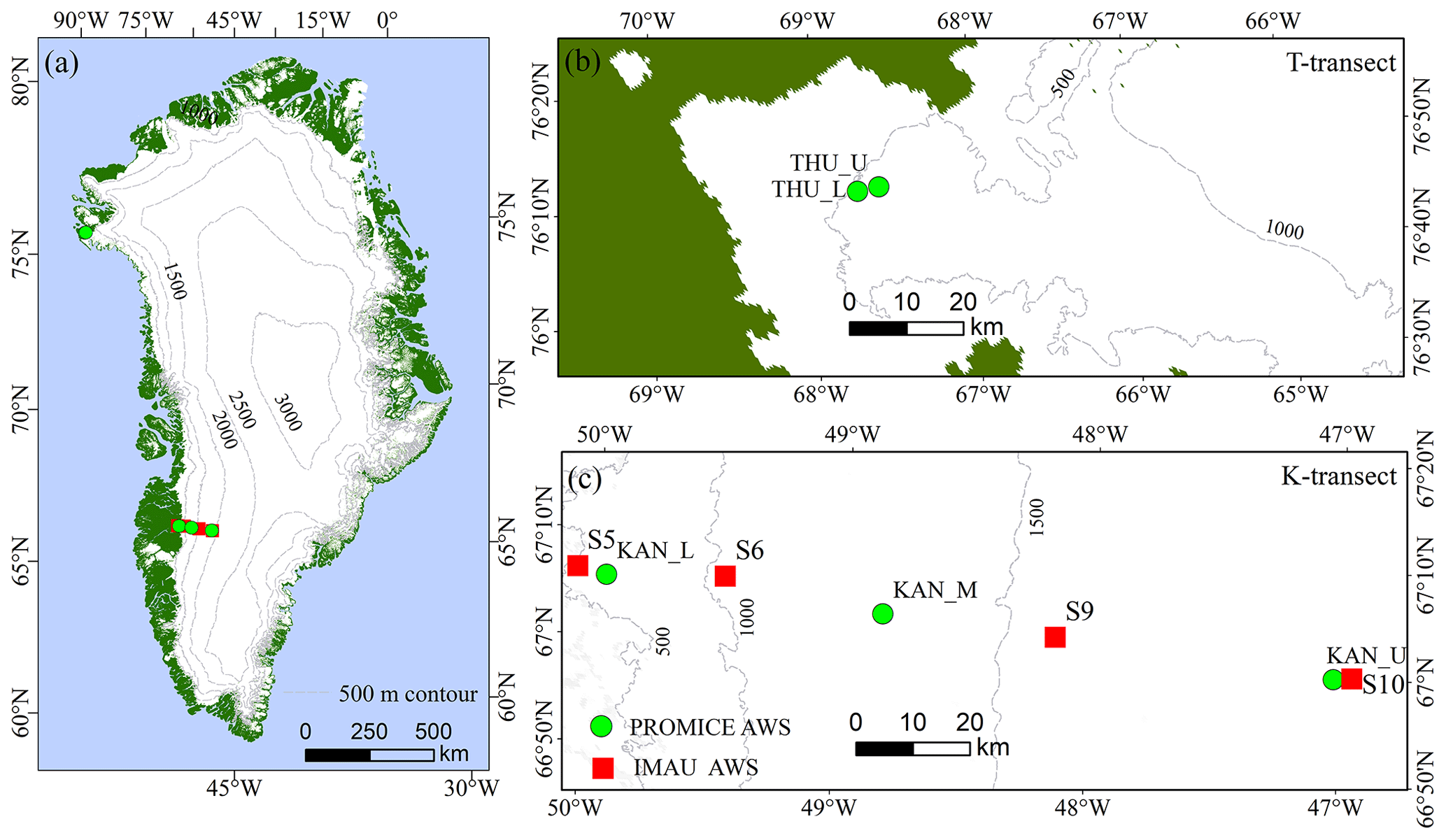
Figure 1 The two GrIS AWS transects used in this study (a): blue represents ocean, green ice-free tundra, and white glaciated areas and location of AWS sites. The transects are magnified in (b) and (c). Red squares are IMAU AWSs and green circles PROMICE AWSs. Dashed gray lines are 500 m elevation contours.

Table 1 AWS location, elevation and start of observations.

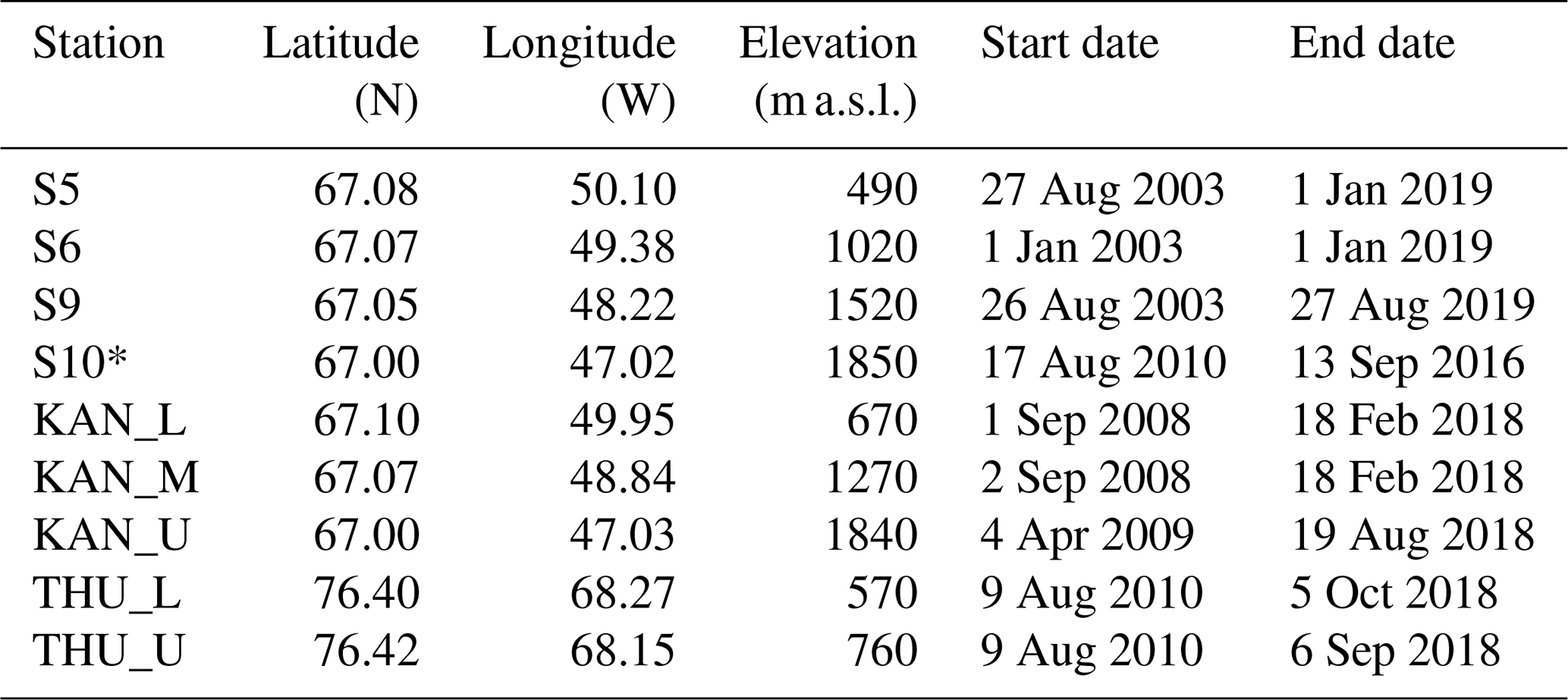
* S10 has currently stopped, while other stations are still operational.

Table 2 AWS sensor specifications. RH signifies relative humidity.

* PROMICE AWS pressure transducer sensor accuracy from Fausto et al. (2012b).

2.2 Data

2.2.1 AWS data and processing

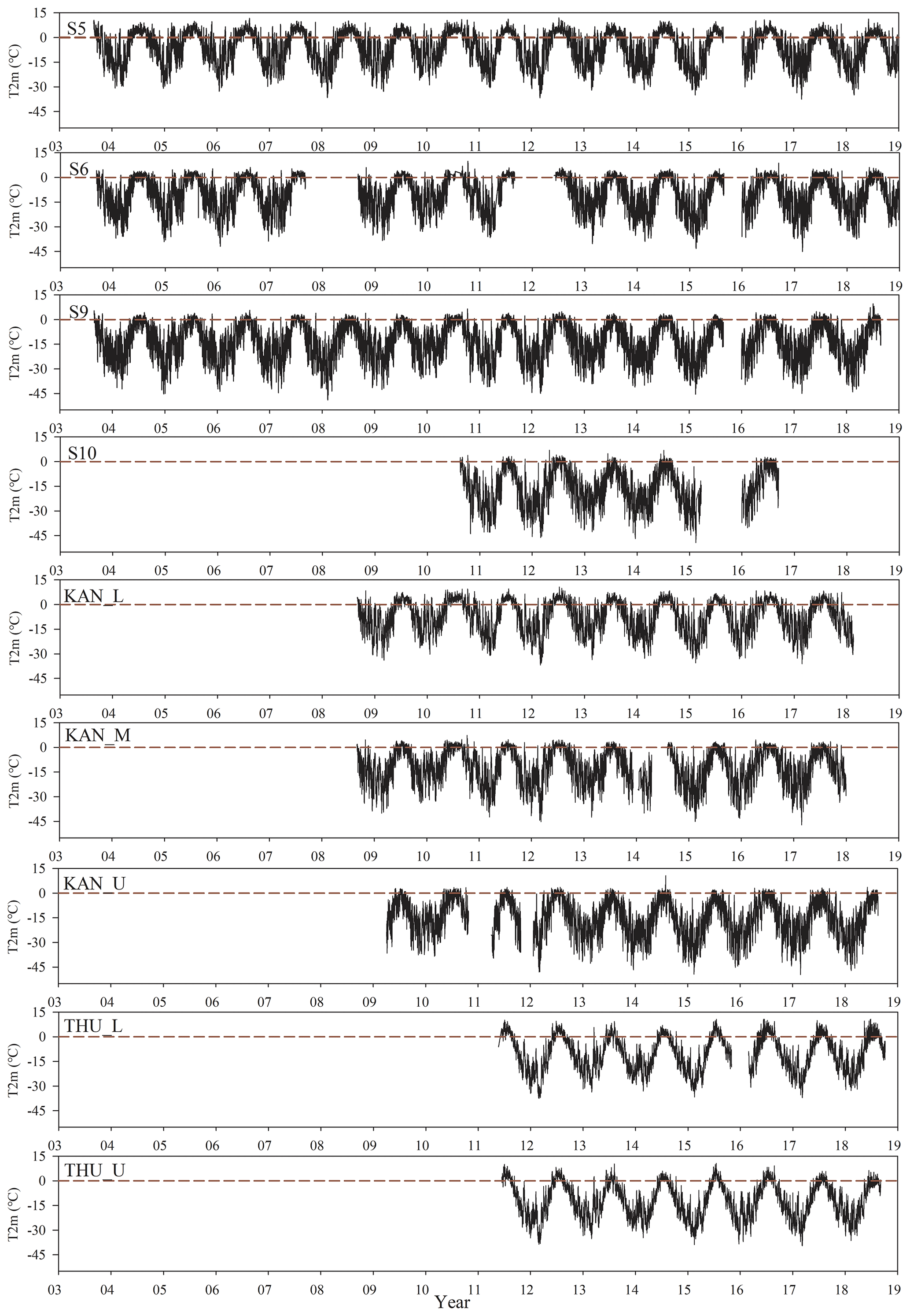
Hourly average wind speed, incoming and reflected shortwave radiation, incoming longwave radiation, air temperature, relative humidity, and air pressure are used to drive the SEB model, and observed emitted longwave radiation is used to evaluate the model performance. The height of the temperature and humidity sensor continuously changes due to ablation and/or accumulation and settling of the station. In order to compare to model output at the 2 m reference height, AWS temperature and humidity are recalculated to this height using the flux-profile relations applied to the turbulent fluxes from the SEB model. To illustrate the data time series at the nine AWSs, Fig. 2 shows the full record of 2 m temperature. Note that S6 data gaps include large parts of 2008, 2010, 2012 and 2015, while the other AWSs have generally more complete coverage.

The sonic height ranger provides changes in the surface height, which allows us to accurately determine snow depth, surface type (ice/snow) for albedo and sensor height required for turbulent flux calculations, as well as for the correction of temperature and humidity values to standard height. Snow and ice height records cannot always be used directly to assess sensor height changes because of AWS design changes and/or settling of the structure. For PROMICE AWSs, we use the results from a physically based method to remove air-pressure variability from the signal of the pressure transducer records (Fausto et al., 2012b; Van As et al., 2011). For details of S5, S6, S9 and S10 data biases, corrections and data gap filling in cases of sensor failure, we refer to Smeets et al. (2018).

Note that AWS time series have differing lengths and completeness. For model evaluation with surface temperature (Fig. 4), we used all available hourly values of emitted longwave radiation; i.e., data points used for Fig. 4 coincide with the time series as shown in Fig. 2. The evaluation utilizing observed ice melt (Fig. 6) uses data starting in 2008 to maximize overlap between the various AWS time series. For the calculation of the average SEB seasonal cycle, we used only complete years (Tables 3 and S1; Figs. 7, 8, 9 and 10).

Figure 2 Time series of 2 m temperature (T_2 m) at the nine AWS sites used in this study.

2.2.2 ERA-Interim and ERA5

The fourth-generation European Centre for Medium Range Weather Forecasts (ECMWF) Interim Reanalysis (ERA-Interim; Dee et al., 2011), available at a spatial resolution of 0.75^∘ and a 6-hourly time resolution, has been widely used over the GrIS (Bromwich et al., 2016; Albergel et al., 2018). ERA-Interim has not continued beyond August 2019 and has been replaced by the follow-on product ERA5. The latter has a higher spatial (31 km) and temporal (hourly) resolution (ECMWF, 2018; Delhasse et al., 2020). Besides the higher temporal and horizontal resolution and updated physics package, the main improvements for ERA5 compared to ERA-Interim are a higher number of vertical levels, an improved four-dimensional variational data assimilation (4D-Var) system and more data assimilation (ECMWF, 2018). In addition to using ERA5 near-surface climate variables and SEB components for evaluation, we also use ERA5 500 hPa geopotential height for the GBI and NAO regression analysis.

2.2.3 RACMO2.3

The Regional Atmospheric Climate Model (RACMO2.3) is developed and maintained at the Royal Netherlands Meteorological Institute (KNMI; Van Meijgaard et al., 2008). The polar version of RACMO2.3 was developed at IMAU to specifically represent the SEB and surface mass balance (SMB) of polar ice sheets such as the GrIS (Ettema et al., 2010). RACMO2.3 incorporates the dynamical core of the High Resolution Limited Area Model (HIRLAM) and the physics from the ECMWF Integrated Forecast System (ECMWF-IFS; ECMWF-IFS documentation, 2008; Noël et al., 2018). We use output at 5.5 km horizontal spatial resolution of the polar version of RACMO2.3 for the period 2003–2018 with a daily time resolution (Noël et al., 2018) for evaluation, as well as monthly 2 m temperature and melt flux data for the GBI and NAO correlation analysis presented in Sect. 2.2.4.

2.2.4 Monthly GBI and NAO index

The Greenland Blocking Index (GBI) represents the mean 500 hPa geopotential height for the 60–80^∘ N, 20–80^∘ W region (Hanna et al., 2014, 2015), while the North Atlantic Oscillation (NAO) index represents the normalized sea level pressure difference between Iceland and the Azores (Hurrell et al., 1995; Jones et al., 2003; Hurrell et al., 2012). The GBI and NAO index time series are made available by the US National Oceanographic and Atmospheric Administration (NOAA)'s Earth System Research Laboratory Physical Sciences Division at: https://psl.noaa.gov/gcos_wgsp/Timeseries/ (last access: 20 November 2019) and are plotted in Fig. 3, in which the blue and red dots represent June, July and August (JJA) values. The two indices are not independent with a correlation coefficient between JJA NAO and GBI values for this period of −0.65; i.e., Greenland blocking is associated with less zonally oriented large-scale flow over the North Atlantic, as expected.

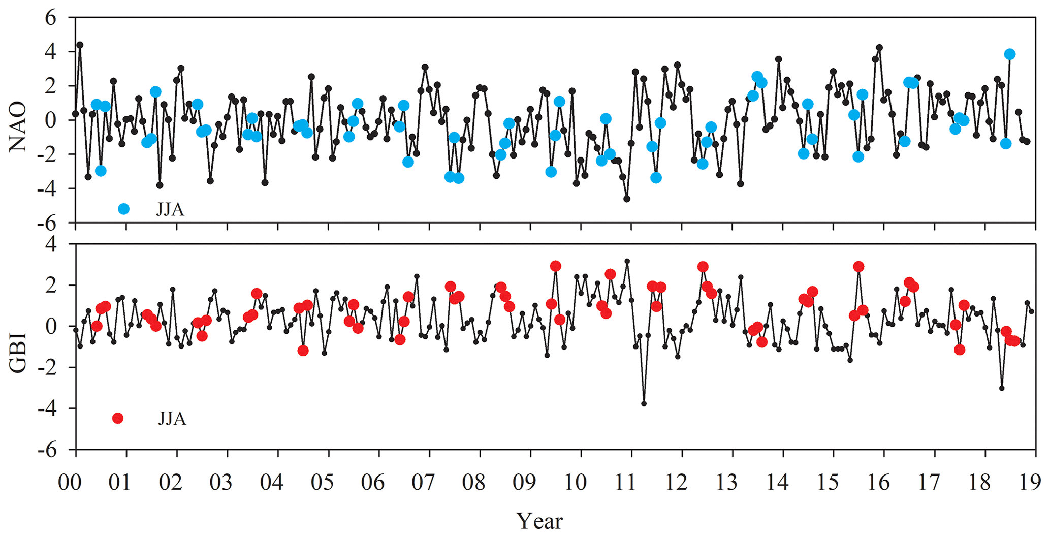
Figure 3 Time series of monthly average NAO index and GBI for which the blue and red dots are values for June, July and August (JJA).

3 Surface energy balance model

3.1 Model description

The surface energy balance (SEB) model uses AWS data as input. It iteratively solves for the value of T_s for which the energy budget is closed.

$$\begin{array}{}\text{(1)}& M+S_{\mathrm{in}}+S_{\mathrm{out}}+L_{\mathrm{in}}+L_{\mathrm{out}}+Q_{\mathrm{h}}+Q_{\mathrm{l}}+G+Q_{\mathrm{p}}=\mathrm{0},\end{array}$$

in which M is the energy used for melt (M=0 when T_s<273.15 K), S_in and S_out are the observed incoming and reflected shortwave radiation fluxes, L_in and L_out are the observed incoming and calculated outgoing longwave radiation fluxes (assuming unit emissivity), Q_h and Q_l are the calculated sensible and latent turbulent heat fluxes, G is the subsurface heat flux evaluated at the surface, and Q_p is the heat flux supplied by rain. All fluxes are evaluated at the surface, and fluxes towards the surface are defined positive. In this study, Q_p is neglected because no information on rainfall timing and rate is available. A previous study used precipitation data from the HIRHAM5 regional climate model bi-linearly interpolated to AWS locations and reported that the rain heat flux on average contributed ∼1 % to the melt flux in summer at the southern GrIS site QAS_L (Fausto et al., 2016).

Q_h and Q_l are estimated using the bulk aerodynamic approach with stability corrections based on Monin–Obukhov similarity theory (Van den Broeke et al., 2005; Smeets and Van den Broeke, 2008) and using the stability functions of Holtslag and de Bruin (1988). The expressions used to calculate Q_h and Q_l are as follows:

$$\begin{array}{}\text{(2)}& {\displaystyle }{Q}_{\mathrm{h}}={\mathit{\rho }}_{\mathit{\alpha }}{c}_p{u}_{\ast }{\mathit{\theta }}_{\ast }={\mathit{\rho }}_{\mathit{\alpha }}{c}_p{C}_{\mathrm{H}}u(\mathit{\theta }-{\mathit{\theta }}_{\mathrm{s}}),\text{(3)}& {\displaystyle }{Q}_{\mathrm{l}}={\mathit{\rho }}_{\mathit{\alpha }}{L}_{\mathrm{v}}{u}_{\ast }{q}_{\ast }={\mathit{\rho }}_{\mathit{\alpha }}{L}_{\mathrm{v}}{C}_{\mathrm{E}}u(q-q_{\mathrm{s}}),\end{array}$$

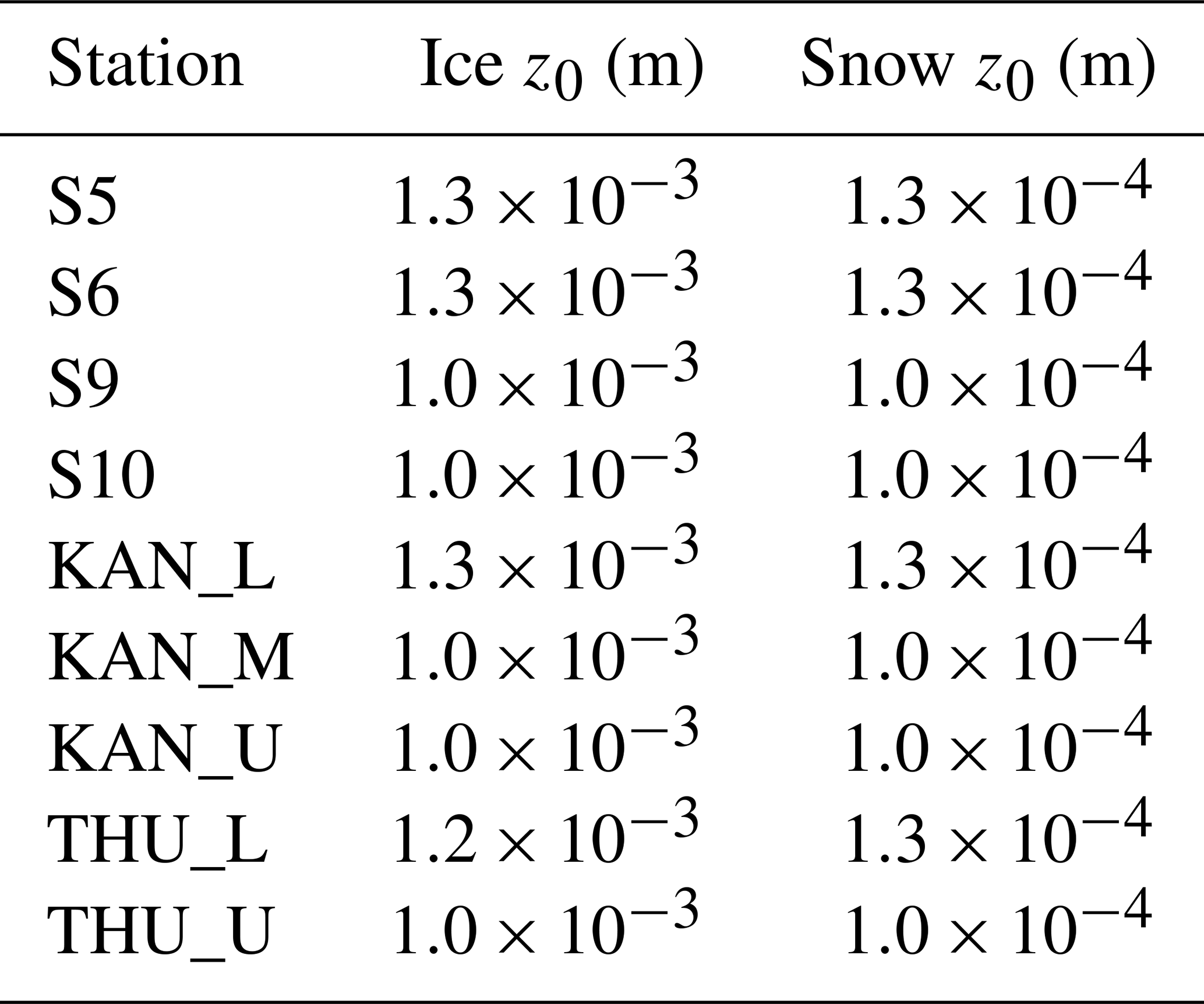
where u_∗, θ_∗ and q_∗ are the turbulent scales for momentum, heat and moisture, c_p is the specific heat capacity of air at constant pressure, ρ_α is air density, L_v is the latent heat of sublimation, and C_H and C_E are bulk exchange coefficients for heat and moisture, respectively. The SEB model uses the measured atmospheric temperature, wind speed and humidity at the AWS sensor level, together with the (iteratively estimated) surface temperature, assuming zero wind speed and saturated humidity values at the surface. The surface roughness length for momentum (z₀) varies strongly in time and space in the ablation zone of GrIS and is often set to different constant values for snow and ice surfaces (Smeets and van den Broeke, 2008; Brock et al., 2006), while the values for heat (z_h) and moisture (z_q) are estimated following the expressions from Andreas et al. (1987). Following the study of Smeets and van den Broeke (2008), a z₀ value of $\mathrm{1.3}\times {\mathrm{10}}^{-\mathrm{3}}$ m is chosen for S5, S6 and KAN_L when ice is at the surface and $\mathrm{1.3}\times {\mathrm{10}}^{-\mathrm{4}}$ m when snow covers the surface at these AWS sites. At S9, S10, KAN_M and KAN_U, we use a constant z₀ value of $\mathrm{1}\times {\mathrm{10}}^{-\mathrm{3}}$ m for ice as the annual cycle is much smaller at these stations (Van den Broeke et al., 2005), while $\mathrm{1}\times {\mathrm{10}}^{-\mathrm{4}}$ m is used for snow. At THU_L and THU_U, we use ice values of $\mathrm{1.2}\times {\mathrm{10}}^{-\mathrm{3}}$ and $\mathrm{1}\times {\mathrm{10}}^{-\mathrm{3}}$ m and snow values of $\mathrm{1.3}\times {\mathrm{10}}^{-\mathrm{4}}$ and $\mathrm{1}\times {\mathrm{10}}^{-\mathrm{4}}$ m, respectively. In addition, determining whether snow or ice is present at the surface is done by combining surface albedo and sonic height ranger data. The z₀ values of all the stations are listed in Table 3.

Table 3 The surface roughness length for momentum (z₀) at the nine AWS sites.

The G calculation uses the vertical temperature distribution in the near-surface snow layers as calculated in the subsurface part of the SEB model, which is based on the SOMARS model (Simulation Of glacier surface Mass balance And Related Subsurface processes; Greuell and Konzelman, 1994) with skin layer formulation (Van den Broeke et al., 2011) in which penetration of shortwave radiation is neglected (Van den Broeke et al., 2011). The subsurface model is initialized using measured density and temperature profiles at the date of station installation and assuming no liquid water. For a more detailed description of the model and recent applications, we refer to Reijmer and Hock (2008), Reijmer and Oerlemans (2002), Van den Broeke (2004, 2008a, b, 2011), and Kuipers Munneke (2009, 2012, 2018).

3.2 SEB model evaluation

The calculation proceeds as follows. The SEB components L_out, Q_h, Q_l and Q_g are expressed in terms of surface temperature, and the SEB model then iteratively searches for the value of T_s at which the SEB is closed. When T_s exceeds the melting point, it is set to 273.15 K, and the remaining energy is used for melting. The root mean square error (RMSE) between hourly modeled and observed T_s values, the latter derived from L_out assuming unit emissivity, is used to evaluate model performance at the nine AWS locations in Fig. 4. The RMSE varies from 1.1 K at KAN_U to 1.6 K at S10. The results show that at KAN_M (RMSE =1.1), KAN_U (RMSE =1.1), THU_L (RMSE =1.2) and THU_U (RMSE =1.1) the model performs better than at S5 (RMSE =1.6) and S10 (RMSE =1.6). Overall, at the nine AWSs, observed and modeled surface temperatures agree largely to within the observational uncertainty.

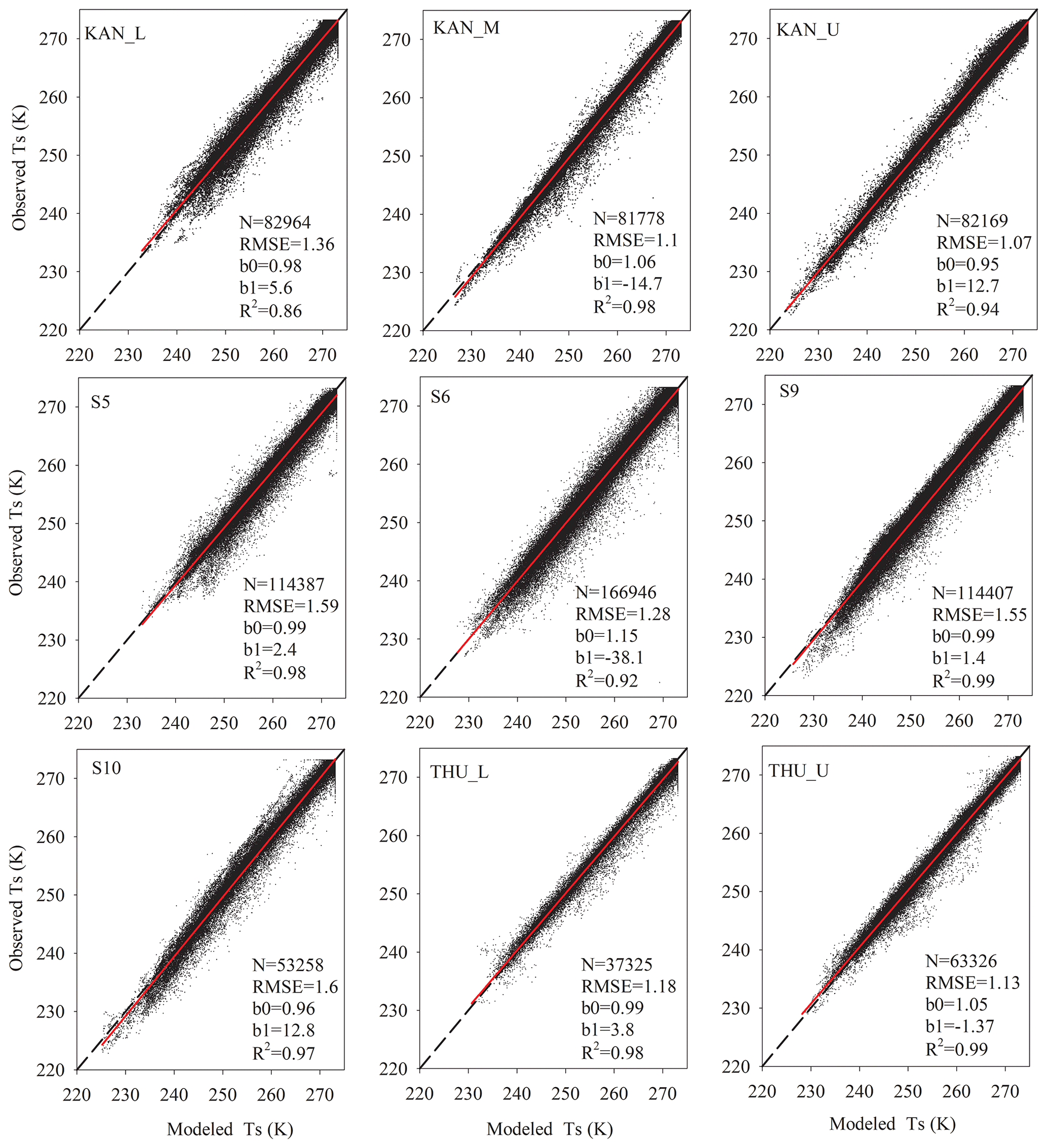
Figure 4 Modeled and observed hourly surface temperature T_s for the nine AWSs. The dashed black line represents the 1:1 line and the solid red line the linear regression. Statistics show the number of data points (N), root mean squared error (RMSE), regression slope (b₀) and intercept (b₁), and coefficient of determination (R²).

When temperature reaches the melting point, it no longer varies in time, and as such it can no longer be used to evaluate SEB model performance. Instead, we assess model performance by comparing observed and modeled ice melt, assuming the density of ice to be known. This does not work for S9, S10 and THU_U, which are situated above the equilibrium line and hence on firn with unknown density. In the accumulation zone, vertical motion of the snow surface can be caused by several processes: changing stake and AWS base depth, differential firn compaction between the stake and AWS base and the surface, and surface mass balance processes that include melt but also, e.g., erosion by drifting snow. Because at the same time the melt fluxes away from the ice margins are relatively small, these processes significantly decrease the signal to noise ratio in the accumulation zone. So even if the density of the layer that has been removed would be perfectly known (which is almost never the case), this cannot be one-to-one converted into a melt flux. For these reasons, modeled melt rate in the accumulation zone is usually evaluated by comparing it to the melt energy obtained from AWS observations. However, this can only be done if the AWSs measure a reliable radiation balance, which limits the effort to the higher PROMICE stations in west Greenland. The resulting scarcity of evaluation points in the accumulation zone warrants caution when interpreting the variability of melt rates in the Greenland interior, as presented in this paper.

A 10 d period is chosen to reduce the measurement noise so that a meaningful comparison is possible (Van den Broeke et al., 2008b). The corrected pressure transducer melt data collected by PROMICE AWSs and SR50A sonic ranger data collected by IMAU AWSs are converted to mass changes (mm w.e.) by assuming an ice density of 910 kg m⁻³. The uncertainty in daily ablation measurements owing to different error sources (differential ablation, density of ice, stake reading) can be as large as ±10 % (Braithwaite et al., 1998). Van den Broeke et al. (2010) report that constant systematic meteorological measurement errors, which can be interpreted as an upper bound on the modeled uncertainty range, result in a model melt uncertainty of ±15 %. Given these uncertainty estimates, with an average difference of 6 % between observed and modeled ice melt, Fig. 5 shows reasonable agreement between modeled and observed 10 d ice melt for KAN_L, KAN_M, S5, S6 and THU_L.

At S5 and S6, Van den Broeke et al. (2008b) and Kuipers Munneke et al. (2018) compared annual ice ablation versus stake observations. They found that although results agreed within the model and measurement uncertainty, the relative differences for individual years could be substantial (up to 20 %). Here, differences for individual 10 d periods of up to 46 % are found, but the average difference is small (6 %).

Figure 5 Average 10 d modeled and observed ice melt (expressed in mm w.e. per day) for the five AWSs situated in the ablation zone, assuming an ice density of 910 kg m⁻³. The dashed line is the 1:1 line and the solid line the linear regression line. Statistics show the number of data points (N), root mean square error (RMSE), regression slope (b₀) and intercept (b₁), and coefficient of determination (R²).

Apart from model uncertainties, there are various possible explanations for the differences. Fausto et al. (2016) show that in the lower ablation area on the southern GrIS (QAS_L), the average rain energy flux in JJA averaged 1 % of the total melt energy flux but can reach 5 %–9 % during high melt episodes. Van den Broeke et al. (2008b) and Kuipers Munneke et al. (2009) used a spectral albedo model based on the parameterization by Brandt and Warren (1993) to calculate subsurface penetration of shortwave radiation at S5 and at Greenland Summit Station. Subsurface melt was only found to be important at S5 but with little influence on the total melt. Based on these results, here we assume that neglecting subsurface radiation penetration in the SEB calculations has little effect on the total cumulative melt flux.

4 Results and discussion

4.1 SEB and comparison of the two transects

4.1.1 Surface height change

The measured surface height change and modeled cumulative ice melt for the seven K-transect stations (S5, S6, S9, S10, KAN_L, KAN_M and KAN_U) are shown in Fig. 6. From 2008 to 2018, the ablation at S5 reached nearly 37 m of ice, while for the stations above the equilibrium line (∼ 1500 m a.s.l.), the total accumulation was about 4 m of firn. At site S5 (490 m a.s.l.), the modeled ice melt and measured surface height change agree well, even in winter, indicating that there is little snow accumulation in winter at this site, as supported by visual observations. At site KAN_L (670 m a.s.l.), there are obvious accumulation events in the winter of 2009 and 2011, and modeled ice melt is generally larger than observed. The strongest melt occurred in summer 2012, contributing to the largest annual ice sheet mass loss on record (Khan et al., 2015; Mouginot et al., 2019; The IMBIE Team, 2019), followed by a return to more average conditions in 2013 (Nghiem et al., 2012; Kuipers Munneke et al., 2018). Overall, modeled and observed total height change agree typically within 10 %.

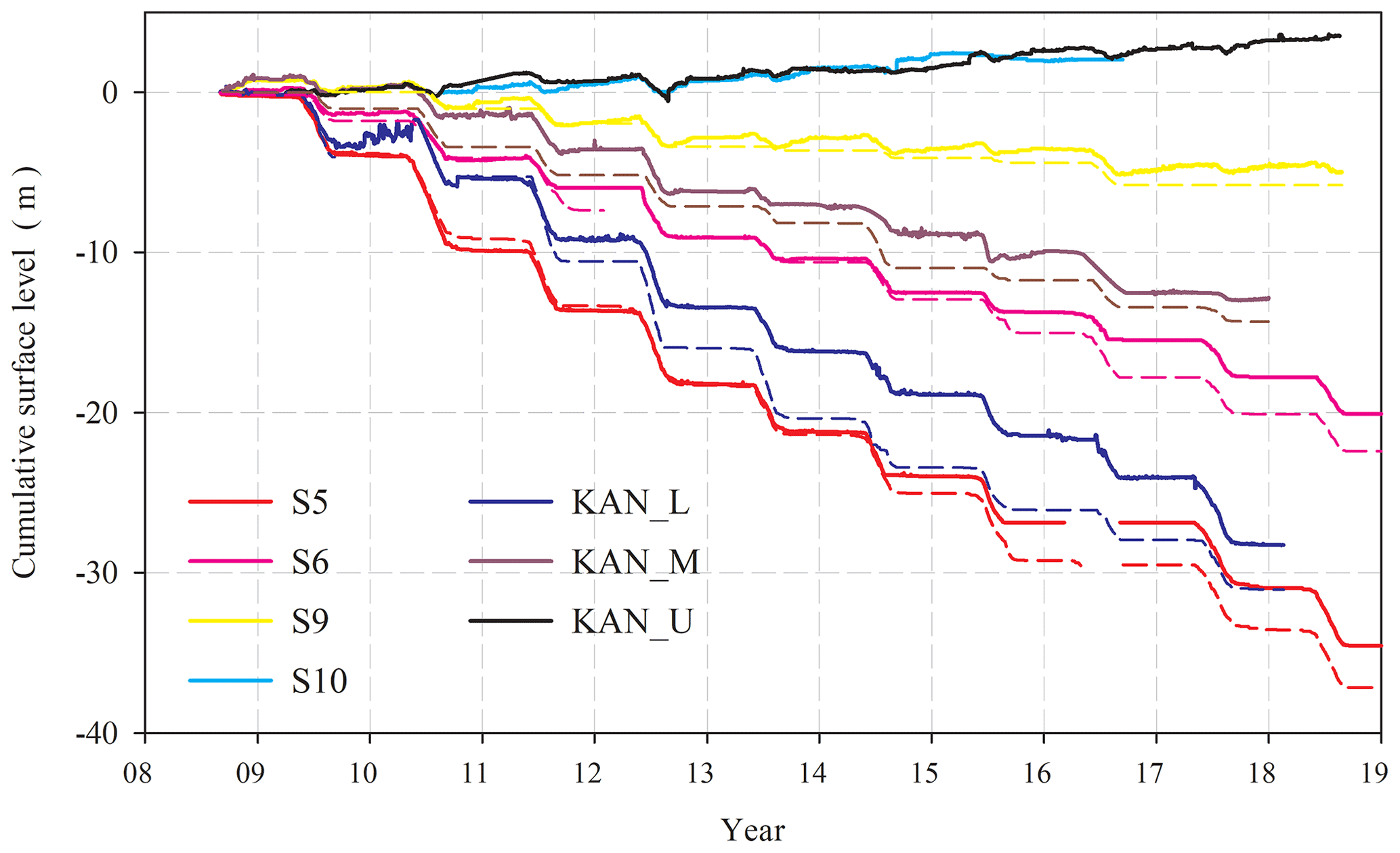
Figure 6 Measured height changes (solid lines) and modeled ice melt (dashed line) at the seven K-transect AWSs.

4.1.2 SEB components

Table 4 shows that average summer (June, July and August; JJA) net shortwave radiation S_net provides most (67 % at S5 to 95 % at S9) of the energy used for heating or melting the surface along both transects (Van As et al., 2012; Van den Broeke et al., 2008b, 2009). On average, S_net is largest at KAN_L (125 W m⁻²) and smallest at S10 (65 W m⁻²). For the T-transect, average S_net decreases from 84 W m⁻² at THU_L to 74 W m⁻² at THU_U. The generally lower values on the northwestern GrIS can be explained by the difference in latitude but also by the smaller value of the shortwave transmissivity (0.63 at KAN_L versus 0.53 at THU_L in summer, using top-of-atmosphere radiation data from ERA5), probably owing to more frequent and thicker clouds along the T-transect (cloud cover 0.51 at KAN_L versus 0.56 at THU_L in summer, using cloud cover estimates from PROMICE AWSs based on L_in and air temperature according to Favier et al., 2004). Along the K-transect, JJA L_in ranges between 250 and 290 W m⁻², while L_out varies between 298 and 314 W m⁻². Along the T-transect, L_in is 273 to 279 W m⁻² and L_out 309 to 312 W m⁻². The reduced longwave heat loss confirms greater cloudiness on the northwest GrIS, which is in agreement with Van As et al. (2012).

Table 4 Energy fluxes (W m⁻²) averaged over June, July and August (JJA) at the nine AWS locations. SEB values of L_out, Q_h, Q_l, G and M are derived from the SEB model, while S_in, S_out and L_in are from observations.

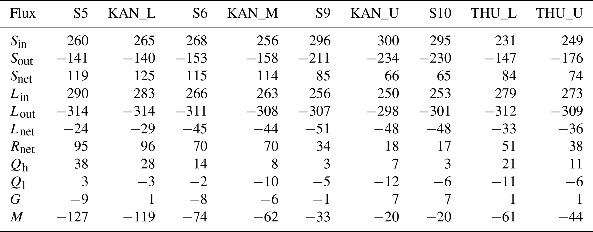
S_net clearly is the main energy source for heating and melt at the ice sheet surface in summer, followed by the sensible heat flux. Q_h is larger than Q_l for the low-elevation stations with a JJA average of 38, 28 and 14 W m⁻² for S5, KAN_L and S6, respectively, indicating significant contributions to the melt energy. At higher elevations, Q_h becomes small and Q_l significantly negative (sublimation) with a JJA average of −5, −12 and −6 W m⁻² for S9, KAN_U and S10, respectively. As a result, above the equilibrium line, the two turbulent fluxes tend to (partly) cancel out. However, summertime S_net and L_net are also negatively correlated, indicating that net radiation R_net is always substantially smaller than S_net. This means that, when compared to R_net, Q_h does provide a significant contribution to summer melt and surface heating energy, ranging from 12 % at S9 to 37 % at S5.

The important role of Q_h in the GrIS SEB becomes even more evident if we look at annual mean SEB components (Table S1 in the Supplement). In winter, Q_h becomes the main source of surface warming. In the absence of absorbed shortwave radiation, wintertime Q_h balances a large part of L_net so that annual mean Q_h is relatively large and annual R_net at S5, KAN_L, S6 and KAN_M becomes small with values of 10, 14, 23 and 6 W m⁻², respectively, even becoming negative for the higher stations (S9, KAN_U and S10). Sites with negative annual mean R_net are very rare at the Earth's surface and require an efficient local atmospheric heat source, which over the GrIS is provided by the mixing of relatively warm air aloft the ice sheet surface by katabatic winds, resulting in large Q_h and large negative L_out. Annual average values of Q_h are as high as 32 W m⁻² at S5, decreasing to 6 W m⁻² at S10, 20 W m⁻² at THU_L and 16 W m⁻² at THU_U. The annual mean latent heat flux Q_l varies between −1 and −6 W m⁻².

Figure 7 shows the interannual variability of the annual melt energy and the corresponding melt water equivalent. The legend lists the percentage contribution from JJA melt for each station. Significant interannual variability is present in the annual melt energy; the standard deviation of the annual melt as a fraction of the average value for stations with >5 years of data ranges from 119 MJ m⁻² (61 % of the mean) at KAN_U to 209 MJ m⁻² (39 %) at KAN_M. For most locations, 2010 and/or 2012 were the strongest melt years, with the highest ablation of 4.8 m w e. per year being reached at S5 in 2010. Only S5 (85 %) and KAN_L (84 %) experience significant (>10 %) non-summer melt; otherwise JJA melt energy contributes more than 90 % to the annual total melt energy. No significant trend is present in any of these time series because they are all relatively short and exhibit large year-to-year variability.

Melt (M) at the K-transect AWS sites is significantly higher than at the T-transect sites; the average annual magnitude of M for THU_L is 512 MJ m⁻² compared to 1160 and 1133 MJ m⁻² for S5 and KAN_L, respectively. Obviously, this can be partly explained by differences in absorbed shortwave radiation caused by the different latitudes of the two transects and the lower temperatures further north, resulting in a shorter ablation season. In the discussion section, we address the potential role of atmospheric circulation.

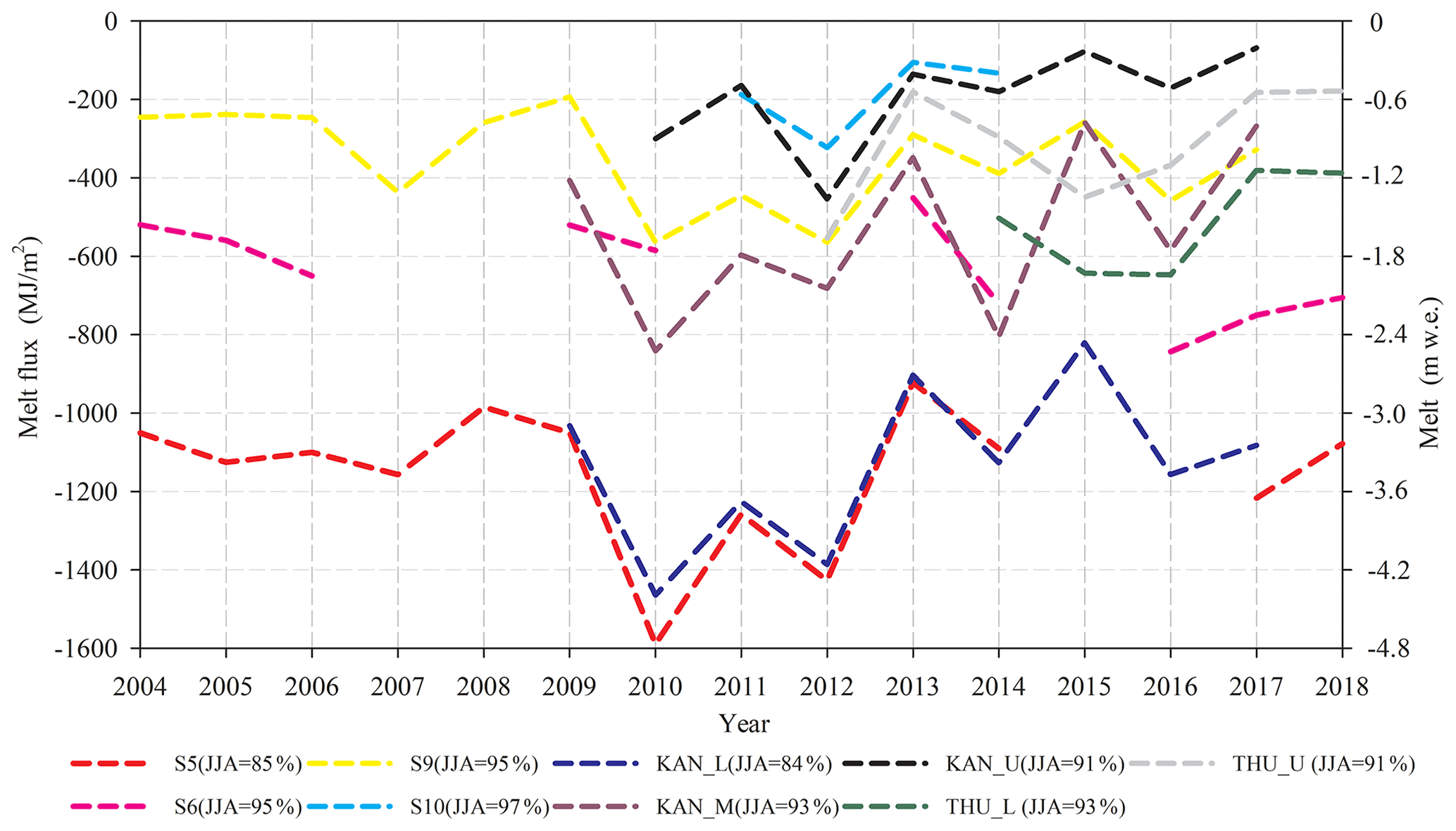
Figure 7 Annual melt energy (2004–2018) at the nine AWS sites and JJA melt energy percentage of the annual total. The dashed line is the annual melt energy (MJ m⁻²), and the right y axis represents the approximate melt water equivalent (m w.e.).

Figure 8 presents the multiyear average seasonal cycle of 2 m temperature, 2 m specific humidity and wind speed at 10 m at the nine AWS sites, while Fig. 9 shows the multiyear average seasonal cycle of SEB components. Temperature and melt peak in July for all sites. Average JJA T_2 m decreases with increasing latitude from 3.0 ^∘C at KAN_L to 1.4 ^∘C at THU_L. The JJA elevational temperature gradient along the K-transect is obvious with 3.7 ^∘C at S5 decreasing to −3.0 ^∘C at S10. Specific humidity increases alongside temperature due to the greater water vapor capacity of warmer air, implying that specific humidity largely follows temperature. Wind speeds are katabatic in nature and generally stronger in winter than in summer for the K-transect AWS sites. The exception is S5 where wind speed shows a double peak because of persistent surface melting in summer, i.e., like a situation in winter with a colder surface and warmer overlying air generating persistent glacier winds. These higher wind speeds enable the highest values for Q_h at S5 as the strong wind shear enhances turbulent mixing in summer in spite of the strongly stable stratification (Fig. 9). The average summertime wind speeds at the T-transect AWSs (7.2 m s⁻¹ at THU_L and 6.6 m s⁻¹ at THU_U) are generally higher than at similar elevations along the K-transect (5.5 m s⁻¹ at KAN_M and 5.8 m s⁻¹ at S10) and show a less well-developed seasonal cycle, possibly owing to stronger synoptic forcing and higher cloud cover which limits surface cooling to drive katabatic flow.

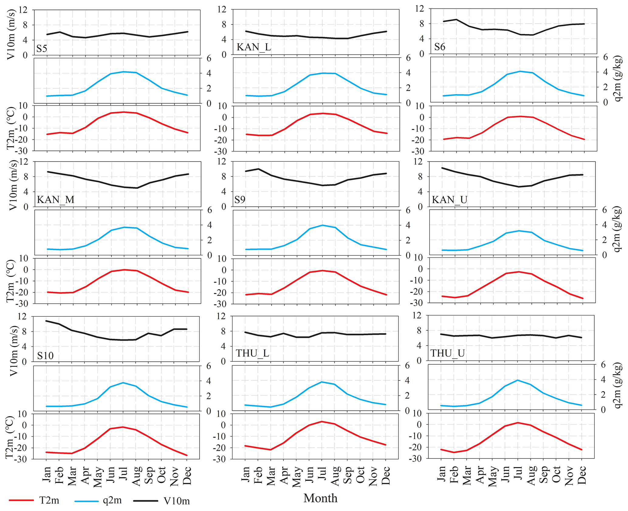
Figure 8 Multiyear average seasonal cycle based on monthly means of 2 m temperature (red, T_2 m), specific humidity (blue, q_2 m) calculated from relative humidity and wind speed at 10 m (black, V_10 m).

Figure 9 shows the seasonal cycle of SEB components. M peaks in July at all sites, mainly following R_net, but July melt differences with June are small at the lower stations (S5 and KAN_L) where low wintertime accumulation means that the albedo assumes the lower ice value early in the melt season, meaning that the main energy source for melt, S_net, peaks at the end of June around the summer solstice. Melting occurs as early as March and lasts until September at S5 and KAN_L, while S6 and KAN_M also experience some melting in September. At THU_L and THU_U, the sharp peak in S_net illustrates the shorter summer melt period.

For the lower AWS sites (S5, KAN_L, S6, KAN_M and THU_L), the shape of the L_net curve is relatively flat or even shows a maximum in summer. This is again a signature of persistent surface melt at these lower sites with the surface temperature limited to a constant 273.15 K, limiting longwave heat loss from the surface irrespective of L_in (Van den Broeke et al., 2011). For the higher AWS sites (S9, KAN_U, S10 and THU_U), a minimum is reached later in spring because the surface is not yet melting and can still increase its temperature (and therewith L_out) in response to the increased absorption of solar radiation (S_net), at least for part of the day.

Figure 9 Multiyear average seasonal cycle based on monthly means of SEB components.

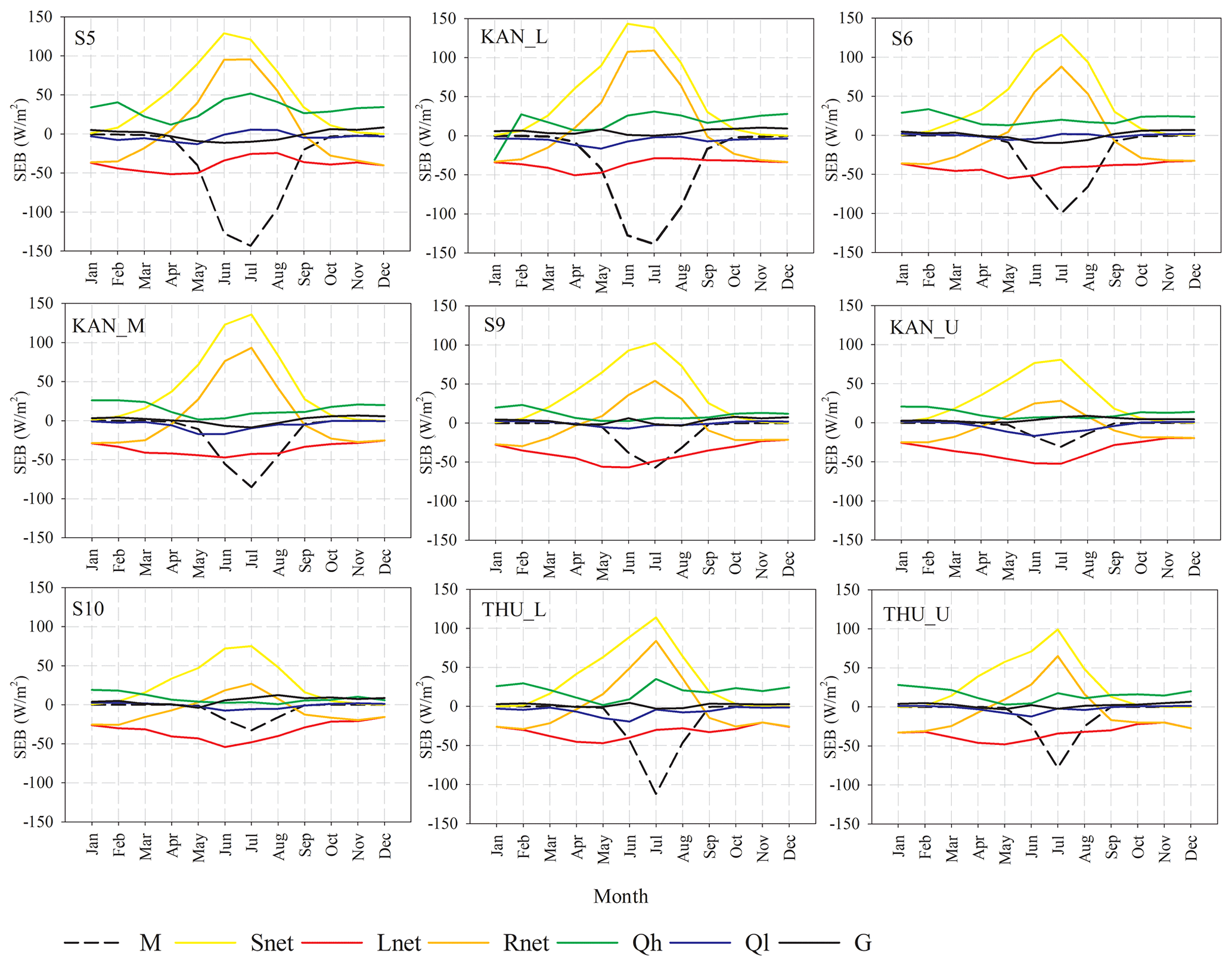
The shapes of the seasonal Q_h cycle at different AWS sites differ significantly. Most stations show a maximum in winter, reflecting that Q_h is the most efficient SEB component to balance L_net; the turbulent cooling of the air over the sloping ice sheet surface results in katabatic winds that effectively mix the near-surface air. In summer, a second maximum occurs at S5, KAN_L and THU_L. These low-lying stations are reached by relatively warm air in summer, as shown in Fig. 8, creating a strong temperature gradient with the melting ice sheet and resulting in shallow katabatic flow (glacier winds) and hence a large Q_h that contributes significantly to melt (Van den Broeke, 1996; Van den Broeke et al., 2005). At S5, KAN_L and THU_L, JJA Q_h averages 45, 28 and 21 W m⁻², respectively, which is at least double that of the more elevated and hence colder inland sites (KAN_M: 8 W m⁻²; KAN_U: 7 W m⁻²). The latent heat flux is generally small and negative, again with the exception of the lowest stations where the persistent melting limits saturation specific humidity at the surface, enabling condensation and making Q_l a small heat source for melting. The strongest sublimation rates are found in spring at the higher stations when the sun heats the surface without it reaching the melting point, enhancing the moisture gradient from the surface to the near-surface air. Seasonal changes in G are small in comparison with the other SEB components.

4.1.3 Variations of surface energy flux with elevation (K-transect)

The seven AWSs along the K-transect enable the construction of robust JJA SEB–elevation profiles (Fig. 10). The average albedos, calculated by dividing the total cumulative JJA values of S_out and S_in, in JJA were all under 0.6 at S5, KAN_L and S6, values were between 0.6–0.7 at KAN_M and S9, and all values were higher than 0.7 at KAN_U and S10. Figure 10 shows that the magnitude of the melt energy M decreases significantly as the elevation increases, from 122 W m⁻² at S5 to 20 W m⁻² at S10, which is in line with S_net which changes from 125 to 65 W m⁻² and with Q_h which decreases from 45 to 3 W m⁻², merely reflecting lower air temperatures and a shorter melt season at the inland sites. Q_l decreases from near zero to being significantly negative (−12 W m⁻²) at S10, reflecting significant surface cooling by sublimation. Net longwave radiation also becomes a more dominant surface heat sink at higher elevations. These profiles are valuable for the evaluation of reanalysis products and (regional) climate models that are used to simulate and predict melting at the surface of the GrIS. For several climate products, this is done in the next section.

Figure 10 Mean June, July and August (JJA) SEB components and albedo versus elevation along the K-transect. Error bars indicate standard deviation in the multiyear annual mean.

4.2 SEB evaluation in ERA5, ERA-Interim and RACMO2.3

We use the results presented in the previous section to evaluate T_2 m, albedo, radiation fluxes, Q_h and Q_l in ERA5, ERA-Interim and RACMO2.3, the latter being forced at the lateral boundaries by ERA-Interim during 2003–2018. We compute model output at the AWS locations with an average distance-weighted interpolation method using the four nearest grid points. Evaluations of KAN_L, KAN_M, KAN_U, THU_L and THU_U are included in the Supplement, and the evaluations of S5, S6, S9 and S10 can be found in Noël et al. (2018). Tables S2–S5 (in the Supplement) show the root mean square error (RMSE), the mean bias (MB) and the correlation coefficient (R) based on linear regressions of daily observations of the PROMICE AWSs.

Although ERA5 better represents the observations than ERA-Interim, the improvement is not statistically significant for all the near-surface variables, which is in agreement with Delhasse et al. (2020). For Q_h and Q_l, RACMO2.3 provides the highest correlations. For THU_U (Table S3), RACMO2.3 shows high correlation coefficients for shortwave fluxes and 2 m temperature, and Q_h and Q_l are also relatively well represented with correlation coefficients between 0.8 and 0.7, higher than both ERA reanalyses. For albedo, ERA5 outperforms ERA-Interim at most stations. This is probably caused by the new snow albedo scheme which changes exponentially with snow age in ERA5 and resets fresh snow albedo, while ERA-Interim sets a maximum constant albedo for snow events (ECMWF, 2018).

We conclude that the regional climate model RACMO2.3 remains a useful addition to reanalysis products for the simulation of GrIS near-surface climate and SEB.

4.3 Relationships with large-scale circulation variability

To better understand the processes driving intra-seasonal and interannual SEB variability in west Greenland, we combine the SEB results presented above with indices of two dominant regional circulation patterns: the Greenland Blocking Index (GBI; Hanna et al., 2015) and the North Atlantic Oscillation index (NAO; Hurrell et al., 1995; Jones et al., 2003).

Figure 11 presents the linear regression slope values of NAO and GBI with monthly mean JJA AWS SEB components and 2 m temperatures (with units W m⁻² or kelvin per 1 standard deviation change in GBI, σ_GBI, and NAO, σ_NAO). The error bars indicate the uncertainty in the regression slope, which generally shows stations along the T-transect having a higher uncertainty than those along the K-transect, mainly caused by the shorter time series in combination with large interannual variability. The associated Pearson correlation coefficients (R) are presented in the Supplement. For instance, Figure S1 shows that significant positive correlations between JJA AWS melt fluxes, T_2 m and GBI are found for all AWSs, whereas correlations with NAO are weaker and generally negative (Fig. S1a, b). For individual SEB components S_net, L_net, Q_h and Q_l, correlations reach significance for some but not all stations, but again they are generally stronger for the GBI than for NAO (Fig. S1c–f).

In Fig. 11, several interesting features can be identified. Starting with GBI (red symbols), we find significantly positive dependencies between JJA AWS melt fluxes and GBI for all AWSs (Fig. 11a). Along the K-transect, the dependency decreases from a maximum of 13 W m⁻² per σ_GBI at S5 to $\sim \mathrm{5}\mathrm{W}{\mathrm{m}}^{-\mathrm{2}}$ per σ_GBI at S10 and KAN_U. The dependencies of the individual SEB components along the K-transect are such that the increase in S_net (Fig. 11c) explains most (40 %–100 %) of this melt increase, which is indicative of clear-sky conditions during episodes of a large positive GBI and is in agreement with previous work (Hofer et al., 2017). Smaller contributions to the melt energy are made by Q_h (Fig. 11e) and Q_l (Fig. 11f). The latter becomes significant because of the limiting effect of surface melt on the surface temperature and hence its (saturated) specific humidity, which decreases the sublimation potential (i.e., making Q_l less negative). L_net (Fig. 11d) contributes positively at the low-lying stations, again owing to the maximized surface temperature during melt limiting L_out, and negatively for the higher stations, which is a result of enhanced surface cooling under clear-sky, non-melting conditions. Surface melt also modulates the 2 m temperature response (Fig. 11b), with a muted response for the lower stations where melt is semipermanent, and larger values at the higher stations, where melt is intermittent.

Albeit with larger uncertainties, consistently high melt sensitivities to variations in GBI of $>\mathrm{15}\mathrm{W}{\mathrm{m}}^{-\mathrm{2}}$ per σ_GBI are found at THU_L and THU_U. Also here, the largest contribution is made by S_net, but we find significant and approximately equal contributions from L_net, Q_h and Q_l. This suggests that in the northwest, high melt under high GBI conditions is associated with high temperatures and cloudiness.

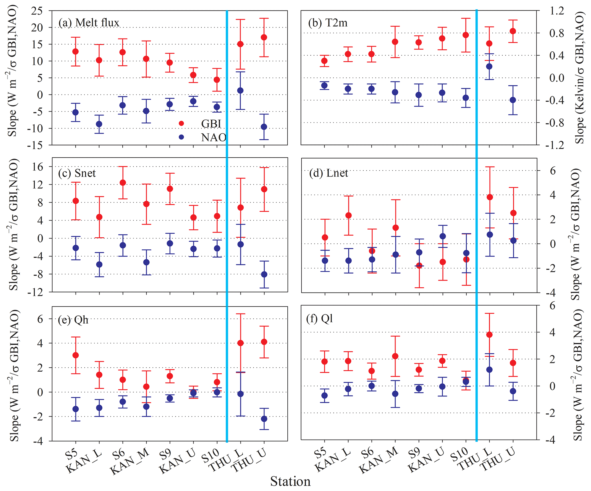
Figure 11 AWS regression slope of JJA average SEB components and 2 m temperature (T_2 m) with GBI (red dots) and NAO index (blue dots). The y axes are scaled with 1 standard deviation change in GBI and NAO circulation index to show (a) the melt flux change from SEB model (in W m⁻² per σ_GBI,NAO), (b) 2 m temperature change from station observations (in kelvin per σ_GBI,NAO), (c) S_net change from station (in W m⁻² per σ_GBI,NAO), (d) L_net change from station (in W m⁻² per σ_GBI,NAO), (e) Q_h change from SEB model (in W m⁻² per σ_GBI,NAO) and (f) Q_l change from SEB model (in W m⁻² per σ_GBI,NAO). Error bars indicate standard error in the multiyear JJA mean.

Next we discuss the spatially different response of western GrIS climate and melt to GBI. To that end, Fig. 12 shows maps of the JJA GBI dependency for temperature (Fig. 12a) and melt (Fig. 12c) for Greenland and its immediate surroundings using RACMO2.3. Figure 13a shows the regional 500 hPa height anomaly from ERA5 associated with variations in GBI. In the latter figure, we use ERA5 since the RACMO2.3 domain does not cover the whole of the Arctic region. Both Figs. 12 and 13 are based on data for the period 2000–2018 (19 years, 57 summer months). Figure S2 in the Supplement shows the correlation coefficient of 2 m temperature and melt flux of RACMO2.3 with the JJA GBI (Figs. S2a, S2c). Figure S2a shows R values for JJA 2 m temperature and GBI of 0.4–0.6 over the southwestern GrIS, which are very similar to the AWS results.

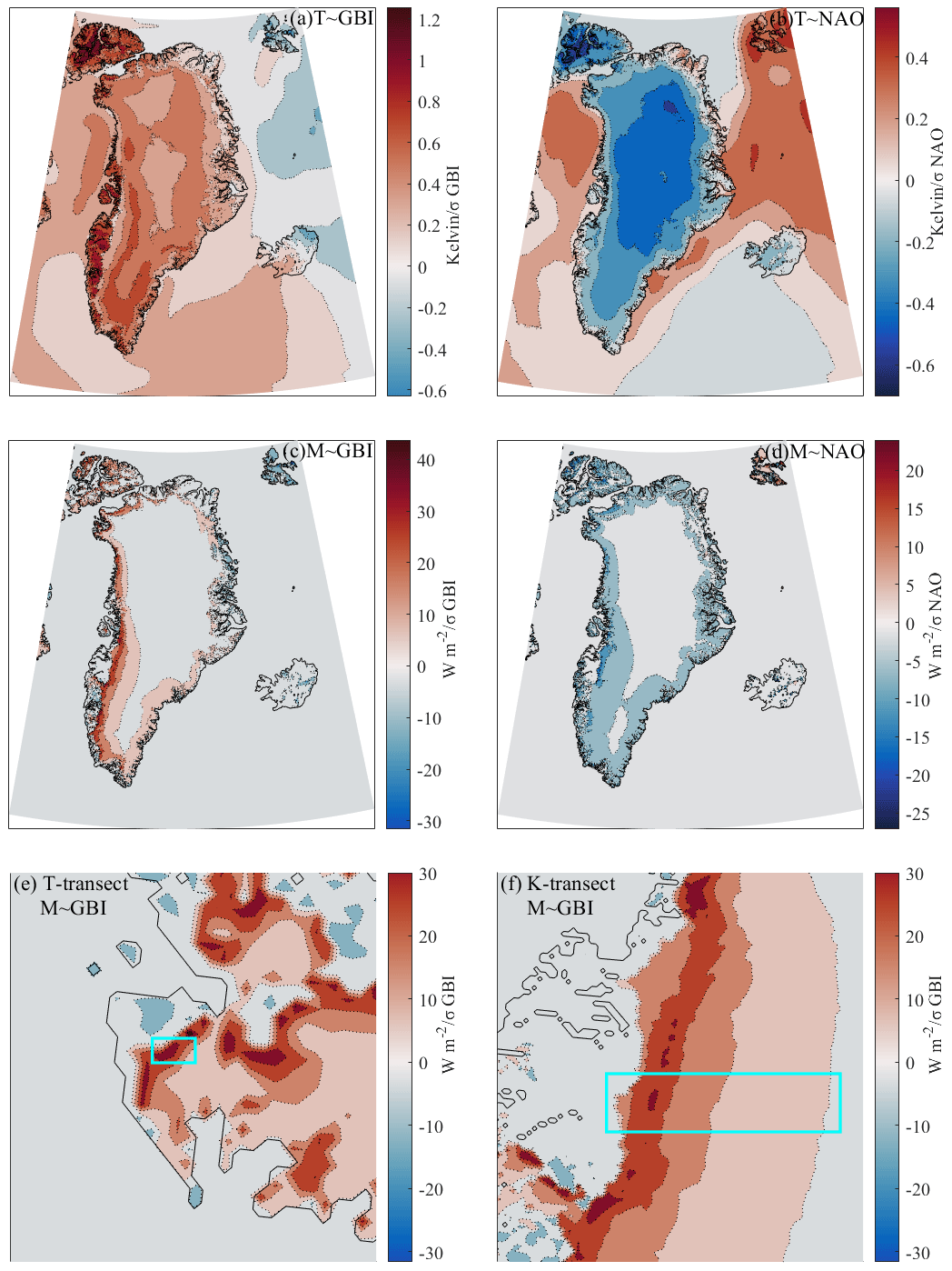
Figure 12 Regression slope of 2000–2018 JJA average 2 m temperature (T_2 m) from RACMO2.3 with (a) GBI and (b) NAO index and melt flux from RACMO2.3 with (c) GBI and (d) NAO index. The regression slope maps are scaled to show the 2 m temperature change from RACMO2.3 (in kelvin) and melt flux change (in W m⁻²) for a 1 standard deviation change in GBI and NAO circulation index. Panels (e) and (f) are enlarged slope value images for T-transect and K-transect of JJA average melt fluxes from RACMO2.3 with GBI. Solid black lines are land–sea mask.

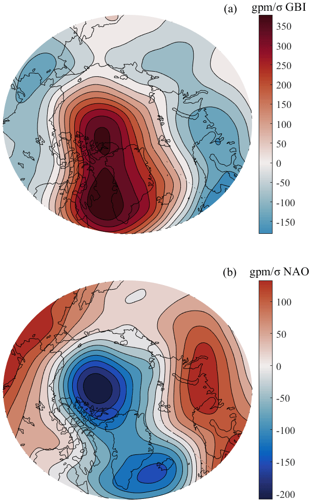
Figure 13 Regression fields slope of 2000–2018 JJA 500 hPa geopotential height from ERA5 regressed with GBI (a) and NAO (b) index. Slope maps are scaled to show the 500 hPa geopotential height change from ERA5 in geopotential meters (in gpm) for a 1 standard deviation change in GBI (a) and NAO (b) circulation index.

Figure 12a and c confirm that the 2 m temperature/melt responses to GBI are dominant in west Greenland and weaker towards the east. The maps also confirm the observed increasing and/or decreasing temperature and melt response with elevation in Fig. 11a and b under high GBI conditions along the K-transect on the southwestern GrIS and the enhanced sensitivity in the northwest (Fig. 12e and f show the enlarged images for melt). Figure 13 shows that the large-scale circulation anomalies for high GBI conditions are very different for the southwestern and northwestern GrIS: the maximum positive anomaly is centered over the K-transect in the southwest, with the largest correlation coefficient R (Fig. S3 in the Supplement) causing clear-sky conditions and a weak or absent circulation anomaly, which explains the dominant contribution of S_net to the melt energy (Hofer et al., 2017). Assuming geostrophy, the circulation anomalies in Fig. 13a imply anomalous southwesterly flow in northwest Greenland blocking conditions. Previous studies confirm that in the northwest during blocking conditions, anomalous southwesterly advection of warm and humid air results in higher temperatures and enhanced cloudiness, which explains the more important contributions made to the melt anomaly by L_net, Q_h and Q_l (Noël et al., 2019).

Since 2007, the GBI has been predominantly positive in summer (Fig. 3), with the exception of low-melt summers in 2013 and 2018, and the strongest positive anomalies are in the strong melt summers of 2012 and 2015 (Hanna et al., 2016). High summer GBI episodes are clearly linked to exceptional GrIS melt years (Hanna et al., 2014), but Hanna et al. (2013), as well as our results, highlight the complexity of the response to summer GBI. Young-Kwon Lim et al. (2016) show that in general, high-pressure blocking primarily impacts the western areas of the GrIS via advective temperature increases. Rimbu and Lohmann (2011) also found strong correlations between winter temperatures across the southwestern GrIS and high blocking activity on the GrIS, whereas Hanna et al. (2013) show that temperatures in Tasiilaq (southeast Greenland) do not show significant correlations with GBI. Here we confirmed and discussed these different responses.

Dependencies of summer AWS melt and 2 m temperatures with NAO are negative and generally weaker (Fig. 11, blue dots), implying a weaker influence of the NAO on western GrIS near-surface climate and melt compared to the GBI. Figure 13b confirms the weaker and less organized impact of NAO on the large-scale circulation in west Greenland with two centers of action in the area of the Icelandic Low in southeast Greenland and a secondary center over the Arctic. Hanna et al. (2015) noted that the more local geographic nature of the GBI means that it correlates more directly with Greenland's climate than the NAO index, and our results support this. Several studies identified a link between anomalously high air temperatures over the GrIS during negative NAO phases (Hanna and Cappelen, 2003; Chylek et al., 2004). A negative NAO index (high air surface pressures in the North Atlantic) is often accompanied by anticyclonic ridging in the GrIS region (Rajewicz et al., 2014). Our results suggest that both GBI and NAO affect the southern GrIS; this part of the ice sheet is wetter during NAO positive phases, while it is drier when GBI is positive. Davini et al. (2012) noted that the geographical dependence of GrIS climate on the NAO shifted eastward, which is consistent with an increase in GBI. Given the large natural, interannual variability, it remains difficult at present to exactly partition the contributions of atmospheric circulation variability and Arctic warming to intensive melting on the western GrIS. Our regression analysis may further help to explain the melting pattern of the western GrIS from the perspective of circulation anomalies (Hanna and Cappelen, 2003; Overland and Wang, 2010; Overland et al., 2012). Also note in Fig. 12 how Svalbard temperature and melt show opposite responses to GBI compared to west Greenland (Young-Kwon Lim et al., 2016).

5 Summary and conclusions

In this study, we forced a surface energy balance (SEB) model with data from nine automatic weather stations (AWSs) situated in the southwestern (seven) and northwestern (two) Greenland Ice Sheet (GrIS). Absorbed shortwave radiation (S_net) is the main energy source for melting (M), followed by the sensible heat flux (Q_h). The multiyear average seasonal cycle of SEB components shows that S_net and M all peak in July but that June is almost a similarly strong melt month for the lowest stations. As the length of the melt season and average albedo in JJA decrease with elevation, so does melt; stations below 1000 m a.s.l. show albedo values <0.6, while the higher stations have values >0.7. Q_h and the latent heat flux (Q_l) also decrease significantly with elevation, and the latter becomes negative at higher elevations, partly offsetting Q_h as a surface heat source.

We used the AWS-derived near-surface climate variables and SEB components to evaluate the performance of two ECMWF reanalysis products (ERA5 and ERA-Interim) and a regional climate model (RACMO2.3). Only for albedo does the newer ERA5 product significantly improve on ERA-Interim. The regional climate model RACMO2.3 has higher resolution (5.5 km) and a dedicated snow/ice module, and it unsurprisingly outperforms the reanalyses.

From the decade-long observational time series, we inferred significant interannual variability in melt energy and SEB components, hiding any significant long-term trend. We report a strong positive correlation of the Greenland Blocking Index (GBI) with western GrIS melt and 2 m temperature, as well as weaker and negative correlations with time series of summertime North Atlantic Oscillation (NAO) index.