Relating regional and point measurements of accumulation in southwest Greenland

In recent decades, the Greenland ice sheet (GrIS) has frequently experienced record melt events, which have significantly affected surface mass balance (SMB) and estimates thereof. SMB data are derived from remote sensing, regional climate models (RCMs), firn cores and automatic weather stations (AWSs). While remote sensing and RCMs cover regional scales with extents ranging from 1 to 10 km, AWS data and firn cores are point observations. To link regional scales with point measurements, we investigate the spatial variability of snow accumulation (b_s) within areas of approximately 1–4 km² and its temporal changes within 2 years of measurements. At three different sites on the southwestern GrIS (Swiss Camp, KAN-U, DYE-2), we performed extensive ground-penetrating radar (GPR) transects and recorded multiple snow pits. If the density is known and the snowpack dry, radar-measured two-way travel time can be converted to snow depth and b_s. We spatially filtered GPR transect data to remove small-scale noise related to surface characteristics. The combined uncertainty of b_s from density variations and spatial filtering of radar transects is at 7 %–8 % per regional scale of 1–4 km². Snow accumulation from a randomly selected snow pit is very likely representative of the regional scale of 1–4 km² (with probability p=0.8 for a value within 10 % of the regional mean for KAN-U, and p>0.95 for Swiss Camp and DYE-2). However, to achieve such high representativeness of snow pits, it is required to determine the average snow depth within the vicinity of the pits. At DYE-2, the spatial pattern of snow accumulation was very similar for 2 consecutive years. Using target reflectors placed at respective end-of-summer-melt horizons, we additionally investigated the occurrences of lateral redistribution within one melt season. We found no evidence of lateral flow of meltwater in the current climate at DYE-2. Such studies of spatial representativeness and temporal changes in accumulation are necessary to assess uncertainties of the linkages of point measurements and regional-scale data, which are used for validation and calibration of remote-sensing data and RCM outputs.

1 Introduction

Numerous recent studies have documented a continuous mass loss from the Greenland ice sheet (GrIS) using remote-sensing data and/or estimates from model simulations (e.g., Shepherd et al., 2012; Velicogna et al., 2014; Khan et al., 2015; van den Broeke et al., 2016; Sørensen et al., 2018; Mouginot et al., 2019). From 1980 to 2018, mass loss from the GrIS increased by a factor of 6 (Mouginot et al., 2019), and over the last two decades the major mass loss process has changed from solid ice discharge to surface mass balance (SMB; Enderlin et al., 2014; van den Broeke et al., 2016; Mottram et al., 2019). SMB can be regarded as the sum of snow accumulation (b_s) and lateral redistribution by sublimation, wind and runoff. Depending on the location, lateral redistribution can increase SMB as well as decrease it. Over most of the GrIS, net accumulation is the dominating factor for SMB (Koenig et al., 2016), while recent negative trends in SMB are related to surface melt and runoff (Vaughan et al., 2013). Despite all advances, SMB estimates remain a major source of uncertainty in ice-sheet mass-balance calculations (van den Broeke et al., 2009). This is because surface mass fluxes, such as snowfall and melt, cannot be measured by remote-sensing technology, and derived estimates based on snowfall can still have significant errors (Bennartz et al., 2019). Hence, predictions of SMB are usually obtained using scarce in situ measurements together with regional climate models (RCMs), which can introduce significant uncertainties (Vernon et al., 2013) as well. Different scales between in situ observations and simulations may also contribute to these uncertainties. The spatial resolutions of RCMs and remote-sensing data are limited to regional scales (on the order of one to tens of square kilometers), while in situ observations cover point data (on the order of a few square meters or less). Effects of wind redistribution, for instance, are leveled out on regional scales but can have significant influences on point scales. As a consequence, evaluation and validation of regional-scale data products using in situ data is difficult without knowledge of the spatial extent and representativeness of the point measurements. To date, only a few studies have investigated how representative point observations (e.g., snow pits, firn cores, mass-balance stake readings, automatic weather station (AWS) measurements) are of the surrounding several square kilometers.

Within the last decade several studies have used radar systems to quantify accumulation variability in Greenland by tracking internal reflection horizons (IRHs; e.g., Dunse et al., 2008; Miège et al., 2013; Hawley et al., 2014; Karlsson et al., 2016; Koenig et al., 2016; Lewis et al., 2017, 2019). While those studies aimed to track IRH variability using data from long ground transects of roughly 100 km (Miège et al., 2013) to more than 1000 km (Hawley et al., 2014) lengths or using airborne-radar data (Karlsson et al., 2016; Koenig et al., 2016; Lewis et al., 2017), only Dunse et al. (2008) linked the point observations from snow pits and cores to the surrounding area. Koenig et al. (2016) used airborne-radar data from NASA's Operation IceBridge to calculate accumulation rates with a stated uncertainty of 14 %, and they compared their results to outputs from an RCM. They compare radar-derived accumulation to two sites with core data, but the locations of those sites are up to 8 km away from the radar track. Hence, it is not possible to identify whether mismatch between the core- and radar-derived accumulations is due to spatial variability or to assumptions in radar-data processing. Systematic offsets in b_s between radar data and RCM outputs, however, occur in northern Greenland with discrepancies between RCMs and radar of up to 30 % (Karlsson et al., 2020). Other recent studies attempt to relate point observations of melt events within the percolation zone of the GrIS to annual atmospheric patterns (Graeter et al., 2018) or determine the mass of percolating liquid water and compare percolation depths observed by upward-looking radar (upGPR) with temperature records in snow and firn (Heilig et al., 2018). In addition, several studies have quantified temporal accumulation variability using ice core records (e.g., Mosley-Thompson et al., 2001; Vandecrux et al., 2019). Since quantification of spatial representativeness of single point measurements for the surrounding square kilometers has only been conducted for one location in western Greenland so far (Dunse et al., 2008), there is a need to explore uncertainties on local and regional scales. The best means of resolving these uncertainties are to increase the spatial coverage of direct measurements (Farinotti et al., 2014) and to improve our understanding of how well point measurements represent a larger area.

Point observations, such as snow pits and ice cores, are usually performed once a year at most. Such temporal snapshots limit the evaluation of spatial representativeness as they can be influenced by recent weather conditions. Hence, it is necessary to clarify whether regional accumulation patterns are consistent over more than one accumulation season to investigate if temporally continuous point measurements such as AWS data, upGPR and neutron probes remain representative.

Meltwater percolation can move mass from snow to the underlying firn (e.g., Charalampidis et al., 2016; Humphrey et al., 2012; Heilig et al., 2018) or even laterally along the surface slope (Humphrey et al., 2012). Hence, surface melt affects SMB (e.g., Sasgen et al., 2012) and accumulation (Heilig et al., 2018). However, it is unlikely that water percolation and mass redistribution are homogeneous on regional scales. Consequently, it is necessary to assess the impact of melt on temporal changes in accumulation distribution for the percolation zone of the GrIS.

The aim of this work is to relate point scales to regional scales of one to several square kilometers in area to improve our understanding of the representativeness of point measurements. For this purpose, we examine snow pit and ground-penetrating radar (GPR) data from two sites within the percolation zone of the GrIS and one site at the equilibrium line gathered over several field seasons. For each site, we investigate density variability between measurements from up to six snow pits within an area of 4 km² made in a single season, process radar transects of up to 25 km recorded in close proximity to those snow pits and spatially extrapolate the radar-derived accumulation to estimate area-wide accumulation variability. For temporal comparisons, we use continuous observations of accumulation and melt recorded by upGPR (Heilig et al., 2018). Our results show that spatial representativeness of snow accumulation for a point measurement (snow pit) is large, but values can be affected by local wind-induced surface roughness. We recommend applying multiple snow depth measurements in the vicinity of the pits to better assess accumulation on regional scales.

2 Methodology

2.1 Test site, instrumentation and data processing

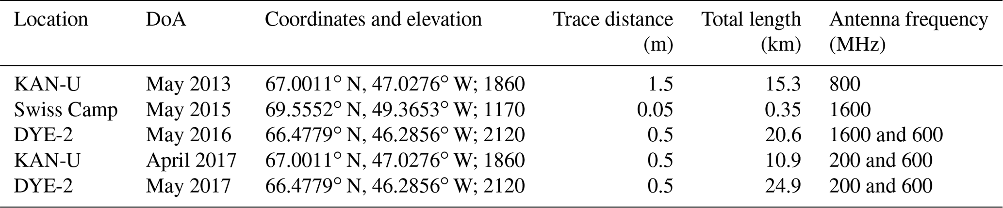
We collected radar data along transects at three different locations on the southwestern GrIS over several years (Fig. 1; Table 1). The sites were visited in the spring of each year (see Table 1). At Swiss Camp a small transect was measured in May 2015 by towing a GPR trolley on foot. The measurements were triggered by an odometer wheel. Geolocation was only performed for the starting and end points of some radar lines, and locations in between are interpolated. We used two different units for the recorded five radar transects. At DYE-2 and KAN-U in May 2017, we employed an IDS (Ingegneria dei Sistemi, Pisa, Italy) FastWave control unit with dual-frequency antennas. The respective frequencies are listed in Table 1. Radar measurements at Swiss Camp in May 2015 and at KAN-U in May 2013 were conducted using a RAMAC system (MALA Geoscience, Sweden). The radar data from Swiss camp have a 0.05 m trace distance along track. The transects at DYE-2 and KAN-U were recorded in time mode and dragging the antennas behind a snow machine. Because small variations in snow-machine speed cause recorded radar traces to be spaced unevenly, the traces are averaged to generate equidistant spacing. The resulting horizontal trace distance is 0.5 m for both DYE-2 transects and the 2017 KAN-U transect. The trace spacing along the 2013 KAN-U transect is 1.5 m because the snow-machine speed was faster. For the DYE-2 and KAN-U surveys, antennas were connected to a GPS receiver for geolocation of the GPR transect.

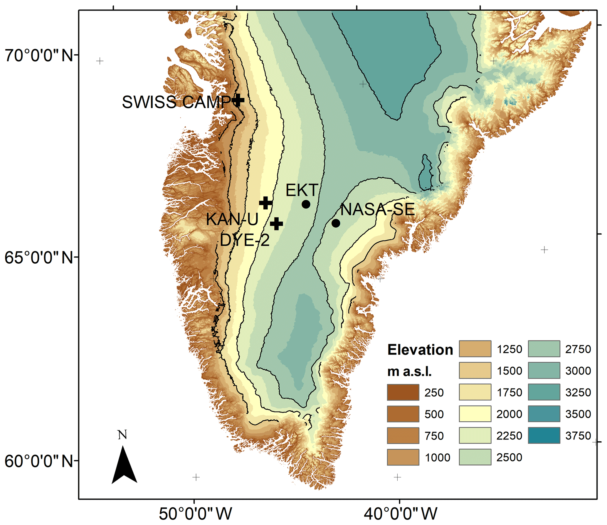
Figure 1 Map displaying locations of radar transects investigated for this study in southern Greenland (black crosses). The black dots indicate additional locations, where snow pits were dug for snow density analysis. The colors are 250 m elevation bands with the maximum elevation per band indicated; the black contour lines are at 500 m intervals. The underlying digital elevation model was generated by Howat et al. (2014).

Table 1 Metadata for the five GPR transects analyzed in this study. Coordinates are presented in geographical coordinates with elevation in meters above sea level (m a.s.l.). DoA is date of acquisition.

All recorded radar traces were processed in a very similar way. In case first arrivals were delayed by more than approximately 2 ns, we started with a correction for the DC shift. We corrected offsets in the zero line of each radar trace (wow) utilizing a dewow function and filtered low- (approximately below 0.5 times the center frequency) and high-frequency noise (approx. above 1.5 times the center frequency) applying bandpass filters. We further applied background removals to minimize disturbing effects from the direct wave and antenna ringing. For all radar transects, we corrected for divergence losses by gain functions and interpolated to equidistant traces. The zero-crossings of the snow surface reflections were corrected to be at time zero.

The measured quantity of radar transects is the two-way travel time (TWT with mathematical symbol τ) from the transmitter to the reflector and back to the antennas (e.g., Heilig et al., 2018). In dry snow and firn (with two contributing volume fractions ${\mathit{\theta }}_{\mathrm{a}}+{\mathit{\theta }}_{\mathrm{i}}=\mathrm{1}$), the wave propagation depends solely on the relation of air (θ_a) to ice volume fraction (θ_i; e.g., Kovacs et al., 1995; Mätzler, 1996). Hence, with the bulk snow density (ρ_s, the average density of the entire snow column) measured in snow pits, we can convert from TWT to snow depth ($\stackrel{\mathrm{‾}}{L_{\mathrm{s}}}$) and the amount of bulk accumulation (b_s with unit kg m⁻²) using the equation

$$\begin{array}{}\text{(1)}& b_{\mathrm{s}}=\stackrel{\mathrm{‾}}{L_{\mathrm{s}}}{\mathit{\rho }}_{\mathrm{s}}\end{array}$$

with

$$\begin{array}{}\text{(2)}& \stackrel{\mathrm{‾}}{L_{\mathrm{s}}}={\displaystyle \frac{\mathit{\tau }}{\mathrm{2}}}{\displaystyle \frac{c}{\frac{{\mathit{\rho }}_{\mathrm{s}}}{{\mathit{\rho }}_{\mathrm{i}}}({\mathit{\epsilon }}_{\mathrm{i}}^{\mathit{\beta }}-\mathrm{1})+\mathrm{1}}}.\end{array}$$

The ice density (ρ_i=917 kg m⁻³), the exponent β=0.5 (related to a medium with random orientation at the microscale), the speed of light in vacuum (c) and the relative dielectric permittivity of ice (ε_i=3.18) are constants taken from previous literature (e.g., Heilig et al., 2018). The reflections of the previous end-of-melt-season (EMS) horizons are clearly detectable in all radargrams. We relate internal reflecting horizons (IRHs) to depths at pit locations using the measured bulk snow density ρ_s within each pit. Accordingly, we choose the zero-crossing of the IRHs as the first break of the respective layer. To identify the EMS horizon of 2015 at DYE-2 in May 2017, we make use of target reflectors that were buried in May 2016 on the 2015 summer horizon. Hence, in May 2017, it was possible to revisit those locations with the radar and unambiguously distinguish between signal reflections arising from the 2015 and 2016 EMS horizons.

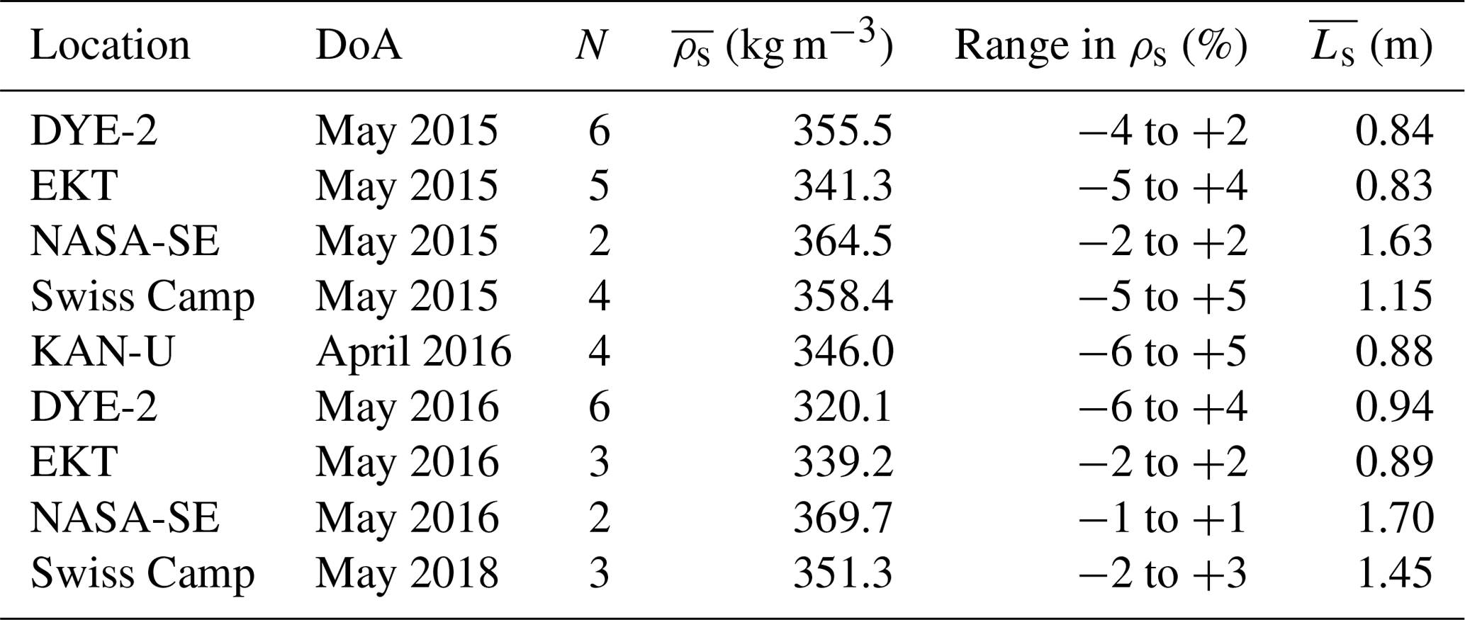
However, before applying a constant ρ_s over the entire length of the radar transects, one has to investigate the spatial heterogeneity in ρ_s over an area of comparable size. To accomplish this, we dug several snow pits at DYE-2 in May 2015 and 2016, at Swiss Camp in May 2015 and 2018, and at KAN-U in April 2016. In each pit, we measured the bulk density of the snow from the surface down to the previous season's melt surface (see Table 2 for details). The snow pits were dug at various distances from each other, at a maximum of up to 1 km apart. In addition to locations where we collected radar data, we also investigated spatial variability in ρ_s at two more sites, EKT and NASA-SE (Fig. 1). As these two sites are located within a distance of 45–60 km of the GrIS ice divide (west of the divide is EKT and east of the divide is NASA-SE; see Fig. 1), they extend our data analysis of spatial variability of ρ_s to the dry-snow zone. The recorded pits at NASA-SE provide data for a high-accumulation site as well. Table 2 displays the numbers of snow pits, the mean density of all pits for that site and year, and the ranges (minimum divided by mean and maximum divided by mean) as percentages. To process the radar data collected at DYE-2 in May 2017, we use density data from firn cores to calculate radar wave speed between the summer 2016 and summer 2015 horizons. Snow temperature measurements ensured dry and subfreezing conditions.

Table 2 Locations of snow density analyses with date of acquisition (DoA), number of snow pits (N), mean density ($\stackrel{\mathrm{‾}}{{\mathit{\rho }}_{\mathrm{s}}}$), density (ρ_s) range as a percent of mean ρ_s and mean snow depth ($\stackrel{\mathrm{‾}}{L_{\mathrm{s}}}$).

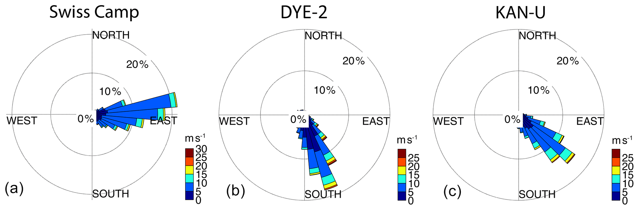
For all three sites, long-term meteorological observations exist. To discuss the meteorological conditions at each site, we use wind data from the GC-Net stations (Steffen and Box, 2001) for DYE-2 (September 2011 to May 2018, with gaps in between) and for Swiss Camp (May 2016 to May 2017) and the PROMICE station (van As et al., 2011) for KAN-U (April 2009 to September 2016).

2.2 Transect data analysis

The measured TWTs of the GPR data are influenced by small-scale surface roughnesses and vertical time sampling. Wind-induced surface features, such as sastrugi, appear in 2-D radar transects as discontinuous, erratic noise. Ideally, we would have performed radar surveys on high-resolution grids (i.e., with spacing smaller than the characteristic length of the features) to spatially extrapolate such features to the unsurveyed areas. However, it was not possible to conduct such high-resolution surveys in the 1 to 2 d available at our sites. Instead, we apply spatial smoothing to minimize artifacts from vertical sampling and to remove wind-induced surface-feature noise.

The time sampling of the recorded GPR transects ranges from 0.05 ns per sample (Swiss Camp 2015) to 0.24 ns per sample (DYE-2 2017), corresponding to approximately 0.006 and 0.028 m per sample, respectively. For the longer transects at KAN-U and DYE-2 (Table 1), the vertical sampling is always coarser than 0.1 ns per sample. As displayed in Fig. 2, the raw radar data for these transects are continuously fluctuating by ±1 sample (corresponding to roughly ±3 cm). Such effects are caused by amplitude clipping of the signal response and uncertainties of the zero-crossing as a consequence of the vertical sampling. For each radar trace, we consistently picked the first strong positive half cycle and shifted the first break upwards to match the zero-crossing. However, due to vertical sample intervals of 0.25 ns, it is likely that the strongest amplitudes shift by 1–2 samples for consecutive radar traces. To reduce effects caused by the amplitude shifts, in our (lower-resolution) KAN-U and DYE-2 data, we applied a Savitzky–Golay filter (Savitzky and Golay, 1964) with a frame length of 20 m and polynomial order of 3 (Fig. 2, yellow line). At Swiss Camp, with the much finer vertical sample interval, it is adequate to filter with a 1 m frame length to reduce clipping and zero-crossing uncertainties.

At Swiss Camp, where we surveyed on a submeter grid, we are able to investigate small-scale accumulation variability directly. For the other two sites, however, the transects were several kilometers in length and not in a regular grid. To enable quantitative geostatistical extrapolation over areas not surveyed with the radar, it is necessary to remove small-scale surface roughness from the data. With a horizontal sampling resolution of 0.5 to 1.5 m, the variability in the radar-derived snow depth is dominated by surface-wind features such as dunes and sastrugi. We determine the average wavelengths and amplitudes of all four longer transects (DYE-2 and KAN-U) by calculating the average distance (in meters) between peaks in snow depth and the arithmetic mean of amplitude of those peaks. The average wavelengths are between 50 and 62 m and amplitudes range between 6 and 8 cm. To filter such surface roughness, we again employ Savitzky–Golay filtering. We search numerically for filter frame lengths for which the average standard deviation within a 20 m radius (below half of the wavelength) around each radar trace is 1 cm or less. The resulting filter frame lengths range from 135 m (DYE-2, May 2016) to 210 m (KAN-U, May 2013), which allowed for the removal of short wavelength variations with an amplitude of about ±0.05 m and more (Fig. 2, green line). A smoothing length of 20 m has been used by other recent studies dealing with large-scale GPR transects as well (e.g., Lewis et al., 2019). We use the smoothed data for spatial extrapolation.

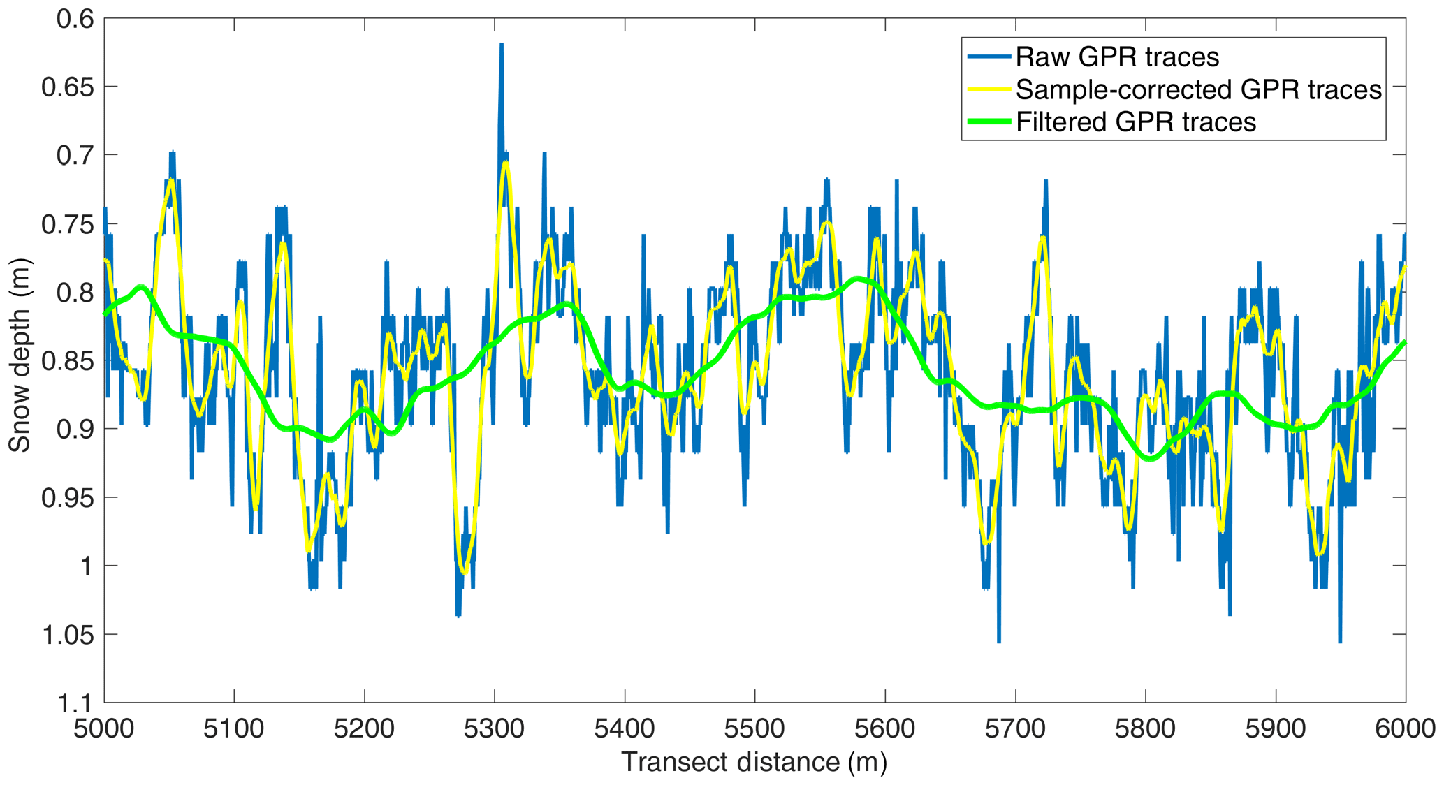
Figure 2 A 1 km section of radar-derived snow depths for the end-of-melt-season 2016 horizon of the radar transect from May 2017 at DYE-2. Displayed are the raw first breaks (blue line), the depths after being corrected for sample uncertainties (yellow line) and the final product being used to assess spatial variability for an area of several square kilometers (green line).

2.3 Spatial extrapolation

In order to analyze accumulation patterns over a larger area, it is necessary to extrapolate the data gathered along the radar transects. One radar trace provides a single depth estimate to a specific reflector. Combining GPR-derived snow accumulation transects with geostatistical techniques is a powerful method to model spatial occurrences of continuous subsurface features. Similar combinations of geophysical and stochastic techniques have been used in previous research (e.g., Rea and Knight, 1998; Tercier et al., 2000). The benefit of radar data is that numerous data pairs for a wide range of measurement distances are recorded, enabling more constrained experimental variograms. Webster and Oliver (2007) state that sample size is directly related to the precision of variogram estimates, while variograms are used to estimate the variance of a parameter (here snow accumulation) at increasing intervals of distance between measurements and in multiple directions. Before spatial extrapolation of a data parameter, the data must fulfill several prerequisites: data have to be spatially continuous and spatially correlated within a specific distance and the expected mean and variance of the data should be invariant in space (e.g., Rea and Knight, 1998). We used experimental variograms to investigate spatial correlation, and snow accumulation at the surveyed sites is spatially continuous (accumulation occurred everywhere within the area of interest, governed by local weather conditions). To ensure that mean and variance are invariant, we investigated trends in the x and y directions separately and subtracted these trends before further analysis. At DYE-2 and KAN-U, we discovered accumulation trends, in both the x and y directions, over the distances surveyed, while, at Swiss Camp, we found a simple one-dimensional trend.

For spatial extrapolation of the univariant parameter snow accumulation, we use ordinary kriging, which is the most robust and most commonly used method (Webster and Oliver, 2007). Ordinary kriging requires normal distribution of the data. Figure 3 displays the probability distributions of all five radar transects. If the distribution (plotted crosses) follows the straight line, the data are normally distributed. At least 10 %–80 % of data match normality for all five GPR transects, and, consequently, no data transformation is applied. We used the Geostatistical Analyst toolbox in ArcGIS 10.4.1 to perform the kriging.

After trend removal, the next step in ordinary kriging is to simulate variograms which adequately mimic the calculated experimental variograms. Standard performance measures to assess the model accuracies are mean prediction errors (values should be at 0 kg m⁻²) and root mean square (RMS) standardized prediction offsets (values should be 1). We present such accuracy assessments in Table 3. In addition, we found directional anisotropy of the covariance in all of the longer transects, which means that correlation ranges of accumulation vary with direction. Hence, we modeled variograms with different correlation ranges per direction. The correlation range marks the limit of the distance between point pairs for being spatially dependent. The major and minor axes of the correlation range ellipsoid used for the variogram modeling are given in Table 3 as well. Swiss Camp is an exception and can be modeled simply by an isotropic variogram. At DYE-2, a spherical variogram model provided the highest prediction accuracies, while at KAN-U and Swiss Camp, the usage of stable variogram modeling resulted in the lowest mean prediction errors and best RMS standardized prediction offsets. The presented correlation ranges in Table 3 represent the direction-wise major extrapolation range. Nugget effects (description of the measurement errors) are small with values below 5 kg m⁻² for all transects. Our kriging outputs have a spatial resolution of 20 m by 20 m for the larger transects and of 0.1 m by 0.1 m for Swiss Camp.

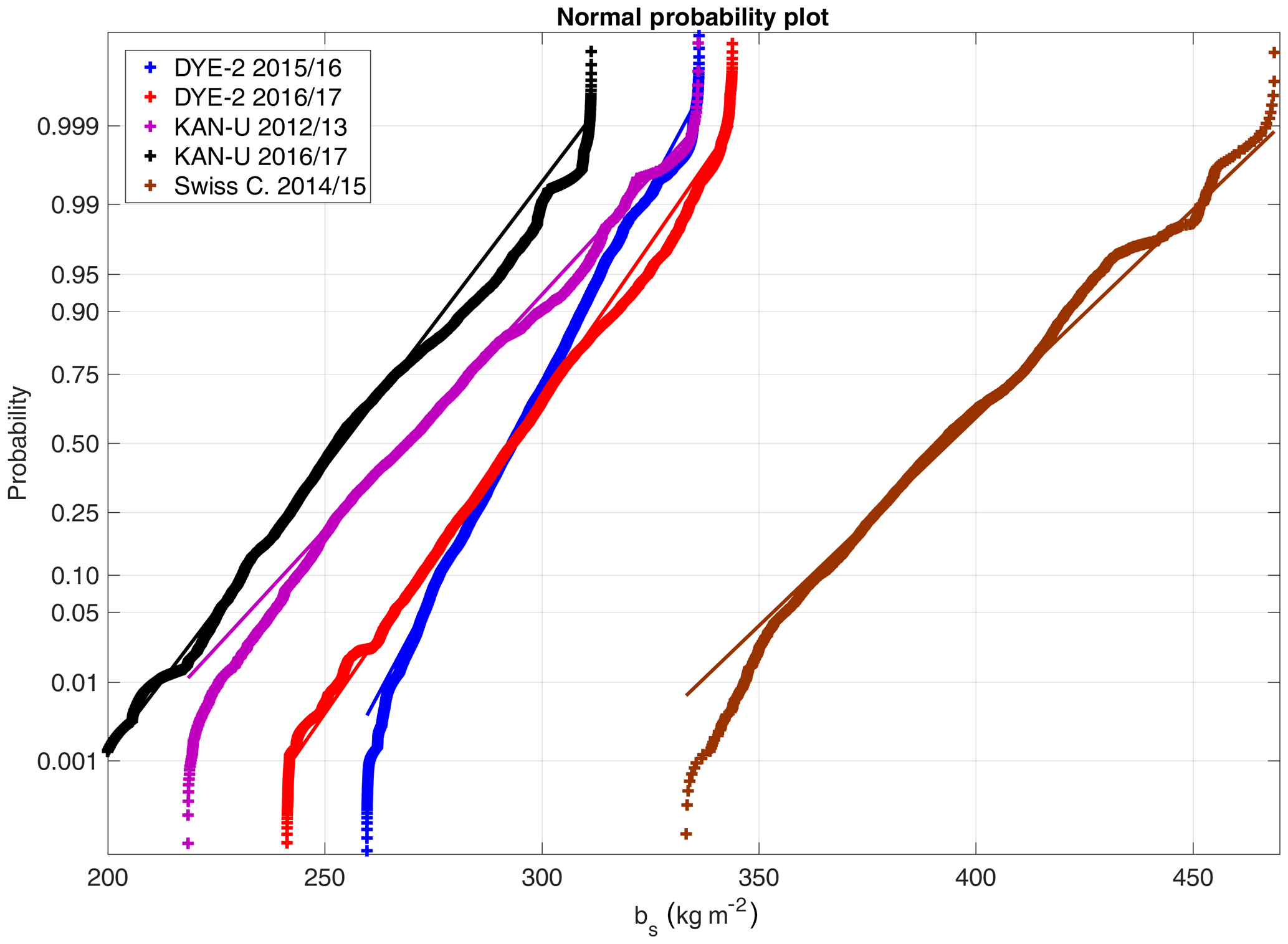
Figure 3 Normal probability plots displaying deviations from a standard normal distribution (straight line with corresponding color). The crosses plot the empirical probability versus the data value for each radar-determined b_s value. We display smoothed transects values for KAN-U and DYE-2 and solely vertical-sampling-corrected values for Swiss Camp.

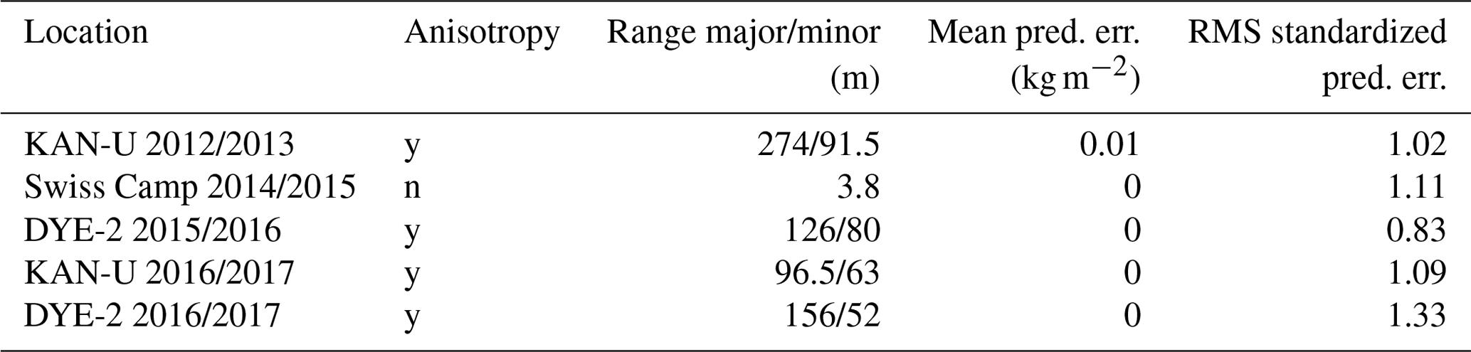
Table 3 Kriging results with description of correlation ranges for the major and minor axes used in the variogram modeling, the resulting mean prediction error (pred. err.), and the root mean square (RMS) standardized prediction error.

To assess the distribution and spatial representativeness of the data, we calculate normalized accumulation values (b_s,N) and normalized cumulative probability distributions. Normalized accumulation is computed such that the individual kriged accumulation value (b_s) is divided by the mean kriged accumulation per site and campaign, $\stackrel{\mathrm{‾}}{b_{\mathrm{s}}}$: $b_{\mathrm{s},\mathrm{N}}=\frac{b_{\mathrm{s}}}{\stackrel{\mathrm{‾}}{b_{\mathrm{s}}}}$. In Figs. 4b, 6c and 7c, data distributions of b_s,N are displayed as box plots with the whiskers set to the 5th and 95th percentiles. Using the recorded radar traces, we determine whether any randomly located point measurement such as a snow pit is representative of the entire extrapolated area. We average all radar traces within a radius of 1 m around each radar trace (which represents a standard pit size) and scale this data point by the mean of the kriged output for the same campaign. Data distributions for each campaign including filtered and sampling-corrected data (see Sect. 2.2) are presented to describe offset dependencies. At KAN-U for the 2012/2013 data, we increase the assumed pit size to an area with a 2 m radius because of sparser horizontal data resolution (1.5 m between traces). Corner locations of radar transects with less than four (three for KAN-U 2012/2013) neighboring traces within the respective search radius are excluded.

3 Results and discussion

We first discuss errors associated with converting measured TWT to accumulation because understanding these errors is essential for assessing how representative a single point observation, such as a snow pit, is of a larger area; we present that assessment in Sect. 3.2. We then evaluate whether accumulation patterns over 2 consecutive years at DYE-2 are different. Finally, we investigate how accumulation changes due to melt and liquid-water percolation. Such effects could be caused by strong lateral differences in melt or lateral flow of meltwater. In the following, to distinguish between offsets, deviations from mean and data distribution, we will describe offsets, deviations and uncertainties of b_s values in percentages (%) and data distribution as probability values of 0–1.

3.1 Error in travel time to accumulation conversion

We investigate the error that we introduce by assuming a single bulk density in the conversion from TWT to snow depth for an entire GPR transect. Hence, we determine the spatial variability in density within the respective area. Table 2 presents snow pit data from our three study sites and two additional sites. The data were collected over 3 years, and the distances between pits ranged from a few meters up to 1 km, while snow depths ranged from 0.83 to 1.70 m. The inclusion of two more sites close to the southern Greenland ice divide extends the data set to a low-accumulation site west of the ice divide (EKT, $\stackrel{\mathrm{‾}}{b_{\mathrm{s}}}\sim \mathrm{300}$ kg m⁻²) and a high-accumulation site east of the divide (NASA-SE, $\stackrel{\mathrm{‾}}{b_{\mathrm{s}}}\sim \mathrm{600}$ kg m⁻²). The range in density variation from $\stackrel{\mathrm{‾}}{\mathit{\rho }}$ in Table 2 – independent of distances between pits – does not exceed −6 to +5 % for nine snow pit campaigns in total, at five different locations for the southern GrIS. Calculated range averages for the last column in Table 2 are −3.7 % to +3.1 %. We thus consider a ±5 % variation in average density to be a robust and conservative estimator of uncertainty within areas of several square kilometers for these regions. This corresponds well with observations by Proksch et al. (2016), who derived a mean measurement uncertainty for density of 2 %–5 %.

Varying ρ_s values only have a small effect on the derived uncertainty of $\stackrel{\mathrm{‾}}{L_{\mathrm{s}}}$ : ρ_s factors into the conversion of τ to $\stackrel{\mathrm{‾}}{L_{\mathrm{s}}}$ as a fraction within the denominator (Eq. 2). For our measured TWTs, a ±5 % variation in ρ_s leads to a 0.7 %–1.4 % uncertainty in $\stackrel{\mathrm{‾}}{L_{\mathrm{s}}}$ for bulk ρ_s values of 200–450 kg m⁻³. Additional uncertainty in $\stackrel{\mathrm{‾}}{L_{\mathrm{s}}}$ is introduced by the smoothing applied to the larger transects. The average RMS deviation in snow depth of the smoothed transects from the sample-corrected transects at DYE-2 and KAN-U is 4.5 cm (5 %–6 %). Combining the errors due to smoothing of radar traces and using a mean density for processing radar transects with observed ρ_s variations using Eq. (1) lead to an average uncertainty in b_s of 7.0 %–7.9 %. This uncertainty is significantly smaller than discrepancies between RCM simulations and Operation IceBridge airborne-radar determinations (16 %; Koenig et al., 2016) and smaller than measured relative standard deviations in density observed within the same study (12 %). However, to increase the robustness of accumulation estimates and to decrease effects of spatial extrapolation, we consider an estimated maximum uncertainty of 10 % in b_s determined from radar data as a conservative estimate for regional catchments of a size of 1–5 km².

3.2 Spatial representativeness of point accumulation

3.2.1 Swiss Camp

Figure 4a shows the measured radar grid and area-wide snow accumulation predicted by kriging for Swiss Camp. In May 2015, we measured a transect length of roughly 350 m with an along-transect resolution of 5 cm and transect lines separated by 60 cm. Radar data were only filtered to remove sample-related noise (see Sect. 2.2), which allows us to identify small-scale variabilities in b_s within 10 cm grid cells. The arithmetic mean of b_s within the surveyed area in Fig. 4a is 393 kg m⁻² with a standard deviation of 28 kg m⁻² (7.1 %). Within the northeasterly part of the presented accumulation distribution (Fig. 4a), we find above-average accumulation. Along the longer transect lines (from south to north), there are several spots with below-average accumulation. Since the extrapolation was performed in accordance to the observed variogram range without boundary conditions being set (snow accumulation outside the measured grid existed; we just do not have information to quantify it), it is impossible to identify minimums and maximums as artifacts or actual variability patterns outside the grid lines. However, the observed minimums in b_s along the south–north transect lines are at regular distances of between 8 and 10 m and are likely the result of wind-generated surface features. Prevailing wind direction is from the east with low variations (Fig. A1a). Along the wind direction, the interpolated area range (east to west) does not exceed 21 m, which is less than the wavelength of the variability pattern observed at DYE-2 (Fig. 2; Sect. 2.2). However, for the cross-wind direction, a wavelength of 8–10 m for dune dips seems to be apparent at Swiss Camp.

Figure 4b displays the normalized accumulation distribution (b_s,N) through box plots. The median (red horizontal line), interquartile range (IQR framed by the blue box), 5th and 95th percentiles (whiskers), and values outside a distribution of p=0.9 (red crosses) are displayed. Similar to the recorded radar data (Fig. 3), a large proportion of extrapolated b_s (p>0.9) follows a normal distribution. In addition, arithmetic mean, median and mode for this data distribution at Swiss Camp are very similar ($\stackrel{\mathrm{‾}}{b_{\mathrm{s}}}=\mathrm{392.5}$ kg m⁻², $b_{\mathrm{s},\mathrm{med}}=\mathrm{391.4}$ kg m⁻², $b_{\mathrm{s},\mathrm{mod}}=\mathrm{381.2}$ kg m⁻²) indicating symmetric data distribution as well (Fahrmeir et al., 2011). A normal distribution, hence a symmetric data distribution, allows direct derivation of distribution probabilities. For instance, the standard deviation for normalized b_s in Fig. 4b is 0.07 which means that a ±7 % deviation comprises p=0.68 of data. However, there is a slight difference in whisker lengths (5th percentile at $b_{\mathrm{s},\mathrm{N}}=\mathrm{0.89}$, 95th percentile at $b_{\mathrm{s},\mathrm{N}}=\mathrm{1.13}$), indicating a small shift towards higher values and asymmetry for the data distribution tales. Skewness of this data distribution equals 0.42. However, p=0.86 of data are within the given ±10 % uncertainty for the entire surveyed area. Consequently, the presented data distribution in Fig. 4b indicates that with a probability of p=0.86, the kriged 10 cm by 10 cm grid points are within 353–432 kg m⁻².

We use the recorded radar traces to numerically analyze how representative any pit location within the ∼400 m² area would be. As described in Sect. 2.3, we define a search radius of 1 m around each radar trace. Radar-derived b_s values are averaged within the search radius. Results are plotted as a normalized cumulative probability plot (Fig. 5). Our analysis shows that with probability p>0.95, any pit location would provide accumulation values within ±10 % of the arithmetic mean for this 400 m² area at Swiss Camp. Only very few pit locations (p<0.05) at Swiss Camp provide b_s values exceeding a 10 % deviation from the arithmetic mean with an overestimation of about 15 % at maximum.

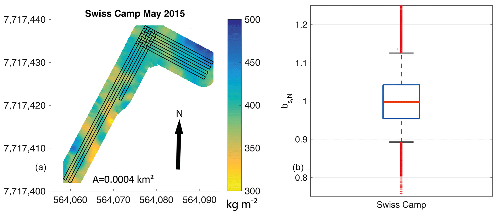
Figure 4 (a) Kriging results for the small radar transect at Swiss Camp for snow accumulation. The black lines display the recorded radar traces, and the black arrow indicates geographic north. A total area of 400 m² can be covered by the applied spatial extrapolation. (b) Box plot displaying normalized data distribution (b_s,N) of kriged output with the red horizontal line showing the median, the box framing the interquartile range, and the whiskers displaying the 5th and 95th percentiles. Outliers are shown as red crosses. The coordinates in (a) are given in UTM zone 22N with datum WGS 1984.

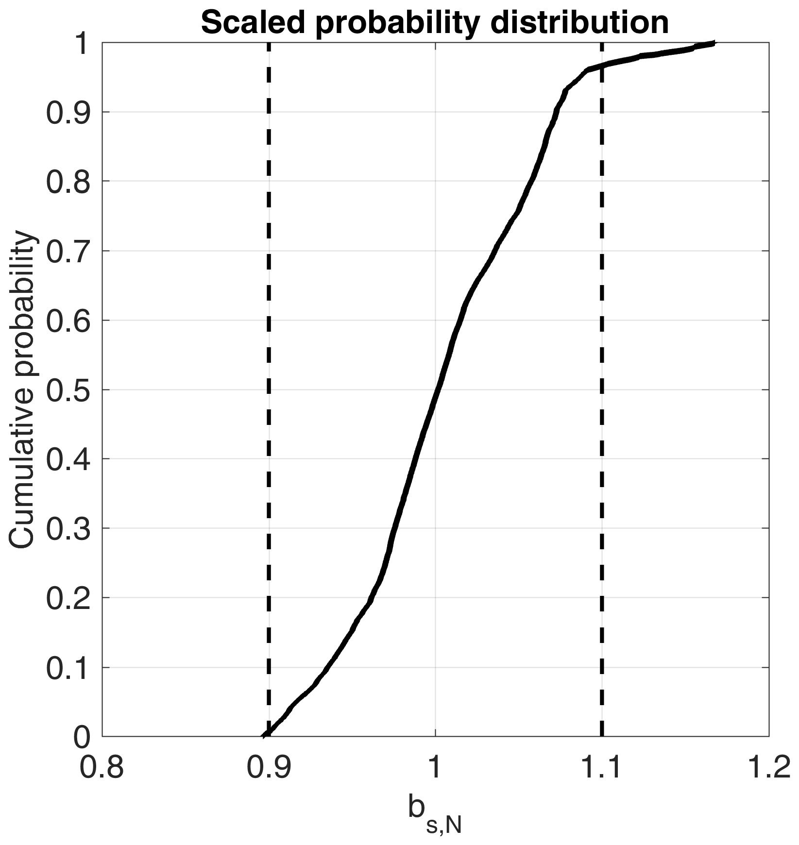
Figure 5 Normalized cumulative probability distribution of radar-derived accumulation (b_s) within any subset with a 1 m radius of the GPR transect at Swiss Camp. The dashed vertical lines represent the determined uncertainty range of ±10 %.

3.2.2 DYE-2 and KAN-U

For the much longer radar transects at DYE-2 and KAN-U, we filtered out wind-induced surface variabilities of the radar traces to increase spatial extrapolation with enlarged variogram ranges from 10–30 to 50–270 m (Table 3). Such filtering implies spatial smoothing of surface roughnesses, which could be performed in the field by extensive snow depth probings. Later in this section, we present comparisons of spatial representativeness of filtered and unfiltered GPR data. In 2016 and 2017, the radar transects were designed to follow the prevailing wind direction to better assess systematic inhomogeneities for DYE-2 and KAN-U in 2017 (see Figs. 6, 7, and A1b and c).

At DYE-2, we recorded 21 km of continuous radar data in May 2016 and 25 km in May 2017. This results in geostatistical predictions of snow accumulation over an area of 2.4 km² for 2015/2016 and almost 4 km² for 2016/2017 (Fig. 6a and b). The arithmetic mean for b_s in May 2016 is 293 kg m⁻² with standard deviation σ=11 kg m⁻². The period 2016/2017 results in almost identical values with a mean accumulation of 296 kg m⁻² and σ=15 kg m⁻².

The box plots in Fig. 6c represent the same quantiles as in Fig. 4b. Data distribution for DYE-2 in 2015/2016 is very homogeneous with an IQR of only ±2.5 %. The whiskers for the same year reach ±6 %. Hence, b_s in May 2015/2016 varies only a little with p>0.9 of data within the uncertainty margins of ±10 %. Since already more than 95 % of radar-derived b_s follows a normal distribution (Fig. 3), values of extrapolated b_s have a high distribution symmetry as well. We observe slightly less homogeneity in the subsequent year at DYE-2. Here, the IQR increases to ±3 %, with the 5th and 95th percentiles being slightly below the error margins of ±10 %. Transforming the named b_s,N values to numbers for b_s in 2015/2016, we observe a likelihood of p=0.9 that all extrapolated 20 m by 20 m pixels range from 275–311 kg m⁻². In May 2017, extrapolated b_s values for an area of 4 km² are at 266–326 kg m⁻² with a likelihood of p>0.9.

The normalized cumulative probability distributions in Fig. 6d demonstrate how representative a randomly located snow pit would be for the entire surveyed area. We analyzed both the sample resolution-corrected radar data (dotted lines) and the filtered data (solid lines; see Sect. 2.2). The filtered data in Fig. 6d indicate that b_s measured in a snow pit anywhere within the radar survey (black lines, Fig. 6a, b) would be within the error margins of ±10 % from the mean of the entire kriged area with a high probability (p=0.99 for winter accumulation in 2015/2016 and p=0.91 for 2016/2017). The unfiltered data, however, show a decreased representativeness with p=0.89 in 2015/2016 and p=0.77 in 2016/2017 for the same uncertainty range of ±10 %. Here, snow depth is solely derived from the snow pit. Such values demonstrate that b_s data derived simply from a snow pit without averaging snow depth for an area around the pit location will decrease the area-wide representativeness at DYE-2.

It is hard to explain the significantly low b_s variability in May 2016 at DYE-2. In theory, low wind speeds could lead to the absence of snow dunes and sastrugi and reduce the spatial heterogeneity of b_s. However, the recorded wind data do not confirm below-average wind for this respective winter season. Determined statistics for wind speeds per winter season (1 October–1 May) at DYE-2 are very consistent over the last 6 years (2011/2012–2016/2017). We can only speculate that a snowfall event 5 d prior to the radar measurements in May 2016 caused the low spatial variability in b_s.

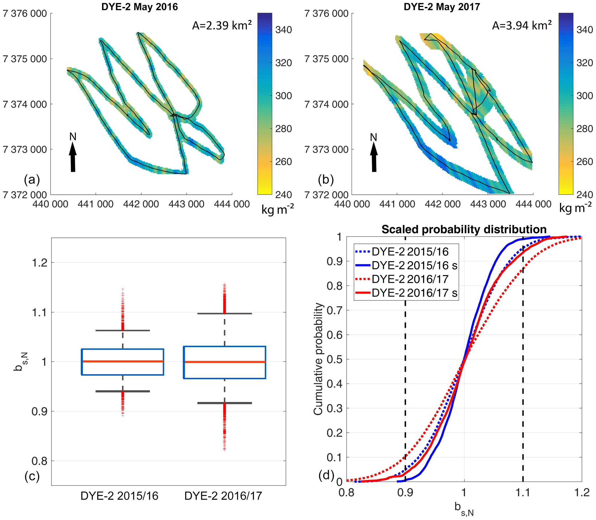
Figure 6 (a, b) Kriging results for the radar transect at DYE-2 for snow accumulation. The black lines show the recorded radar traces, and the black arrows indicate geographic north. The letter A is the total area covered by extrapolation. (c) Box plots displaying normalized data distribution (b_s,N) of kriged outputs with the red horizontal line showing the median, the blue box framing the interquartile range, and the whiskers displaying the 5th and 95th percentiles. Outliers are shown as red crosses. (d) Normalized cumulative probability distribution of radar-derived b_s within any subset with a 1 m radius of the GPR transects. The dashed vertical lines represent the determined error margins of ±10 %. Compared are filtered (solid lines and letter s) with unfiltered (dotted lines) radar transects. All map coordinates are given in UTM zone 23N with datum WGS 1984.

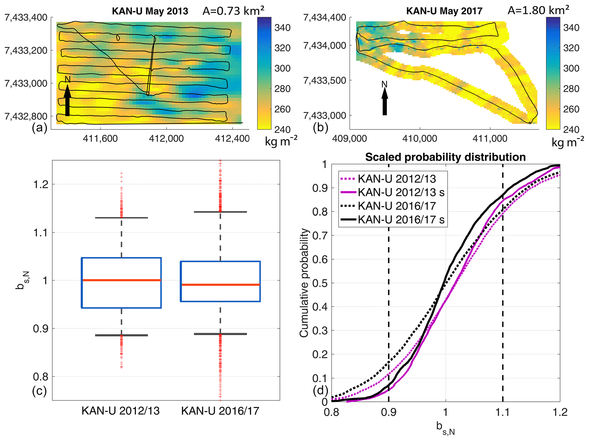
Figure 7 (a, b) Kriging results for the radar transect at KAN-U for snow accumulation. The black lines show the recorded radar traces, and the black arrows indicate geographic north. The letter A is the total area covered by extrapolation. (c) Box plots displaying normalized data distribution (b_s,N) of kriged outputs with the red horizontal line showing the median, the blue box framing the interquartile range, and the whiskers displaying the 5th and 95th percentiles. Outliers are shown as red crosses. (d) Normalized cumulative probability distribution of radar-derived b_s within any subset with a 1 m radius (3 m radius for 2012/2013) of the GPR transects. The dashed vertical lines represent the determined error margins of ±10 %. Compared are filtered (solid lines and letter s) with unfiltered (dotted lines) radar transects. All map coordinates are given in UTM zone 23N with datum WGS 1984.

At KAN-U, the transect lengths and area coverage differed greatly between May 2013 and May 2017 (Fig. 7a, b). The 2013 survey covered an area of 1 km² with a transect length of more than 15 km. In 2017, our radar surveys were approximately 11 km in length resulting in extrapolated area coverage of 1.8 km². The average winter accumulation for the entire area is at 272 kg m⁻² (σ=20 kg m⁻²) in 2013 and 253 kg m⁻² (σ=19 kg m⁻²) in 2017.

The box plots in Fig. 7c demonstrate a more variable data distribution at KAN-U than at the other two sites. The IQR for extrapolated b_s in 2012/2013 is at −6 to +5 % around the arithmetic mean. In 2016/2017, the IQR decreases to ±4 % around the mean. For both years, the whiskers reach outside the error margins of ±10 % and, consequently, indicate less than p=0.9 of data being within the error margins at KAN-U (p=0.82 for 2012/2013 and 2016/2017). Accumulation data of 2016/2017 have a higher skewness of 0.37 in comparison to 2012/2013 (skewness of 0.17). Similar to the recorded radar data (see Fig. 3), the upper quartile in b_s is right-shifted towards higher values. This is due to the homogeneous peak in accumulation at the northeastern corner of the grid (Fig. 7b). Here, we measured above-average b_s, which consequently led to above-average interpolated values. The larger spatial heterogeneity in accumulation at KAN-U than at DYE-2 and Swiss Camp results in snow pits being slightly less representative of the surrounding area; only 80 % of the respective May pit locations would provide area-wide b_s values that are within a 10 % error (for both accumulation seasons). Again, if snow depth is not averaged around pit locations, the likelihood of representing area-wide b_s decreases to p=0.68 (2012/2013) and p=0.64 (2016/2017).

Not all of the recorded radar transect grids are ideal for the applied geostatistical analyses. The distances between radar lines at DYE-2 and KAN-U in May 2017 are too large to allow interpolation between the lines. We had limited time available for radar surveys, and we chose to focus on surveying larger areas (up to 20 km²) instead of only surveying dense grids. The results presented in Figs. 6b and 7a give us confidence that the data gaps do not include major dips or peaks in snow accumulation because no such inhomogeneities exist within the areas of good spatial coverage.

The above results imply that a point measurement of b_s (snow pit, upGPR value, neutron probe, etc.) is representative of an area of roughly 4 km × 4 km at DYE-2 with a probability of p≥0.9 and an uncertainty of ±10 % in cases where snow depth is averaged. For KAN-U, the spatial variability is slightly higher, and, consequently, there is less certainty about how well a single measurement represents the surrounding area. However, we consider a probability of p≥0.8 with uncertainty of ±10 % for both study sites as a resilient estimate.

To quantitatively assess the benefit of snow depth measurements in addition to a snow pit, we numerically assume a sinusoidal snow depth variation with wavelengths of 56 m (arithmetic mean of the previously presented range in wavelength for the GPR transects) and an average amplitude of ±6.8 cm (the fluctuations in snow depth from arithmetic mean). Averaging multiple snow depths (with a sampling distance of 1 m) from a 20 m long probing transect results in a maximum possibly measured offset in snow depth of −20 % (amplitude decreases to 5.4 cm). A 10 m long probing line reduces the maximum offset by −6 % compared to single point measurements (6.4 cm amplitude). A 30 m long snow probing line, however, results in a decrease of maximum possible offsets by −44 % (3.8 cm amplitude). An additional cross line of probings will further decrease offsets. Only if the surface features are aligned symmetrically in both probing directions, the maximum offset derived from both lines will theoretically remain stable. For a measured snow pit with ρ_s=350 kg m⁻² and $\stackrel{\mathrm{‾}}{L_{\mathrm{s}}}=\mathrm{1}$ m, the combined regional uncertainty (±5 % density uncertainty, ±6.8 cm snow depth variation) reduces from a single point measurement with $b_{\mathrm{s}}=\mathrm{350}\pm \mathrm{42}$ kg m⁻² to a maximum possible uncertainty of $b_{\mathrm{s}}=\mathrm{350}\pm \mathrm{35}$ kg m⁻² for just a single 20 m probing line. These numerical results confirm values for representativeness derived from geostatistical extrapolation. Hence, we recommend combining a larger number of snow depth probings within an area of at least 20 m by 20 m in the vicinity of the pits to increase the regional representativeness. Regional snow density variations of ±5 % can be accepted if snow depth uncertainty is minimized. Snow probing lines can easily be performed with relatively low time consumption compared to multiple snow pits. In particular, the wind-induced surface roughness has to be accounted for to provide spatially representative b_s values.

Averaging radar traces within a 1 m radius results in a pit size of roughly 3 m². This is slightly too big for conventional pits with on average a 1 m snow depth. However, the search radius is related to the horizontal data resolution of the radar traces and had to be further increased for the KAN-U site in 2012/2013.

3.3 Interannual changes in accumulation patterns

At KAN-U only 0.16 km² was covered during both radar acquisitions, and, consequently, we do not investigate changes in accumulation for spring 2013 and 2017. For DYE-2, we recorded radar transects for two consecutive winter accumulation seasons. However, multiyear intersecting radar transects and, hence, spatially consistent area-wide b_s estimates are reduced. The intersecting area at DYE-2 comprises roughly 1.7 km². Here, we observe a slight trend in the north–south direction for both accumulation seasons (Fig. 6a and b). While the most southerly parts of the transect show b_s values that are above area-wide average, the northern fringes are below the arithmetic mean of the area in b_s. However, for both years the trends (in a north to south direction) are statistically nonsignificant and very low at 5 kg m⁻² per 1 km for 2015/2016 and 8 kg m⁻² per 1 km for 2016/2017. The respective coefficients of determination of accumulation with latitude are very low as well (R²=0.15 for 2015/2016 and R²=0.25 for 2016/2017). The parallel stripes, mainly visible in Fig. 6b for the southern parts, are certainly artifacts provoked by the grid design and the applied kriging. Local maximums in regular distances (150–220 m) occur along the transect line; however, the spatial extrapolation of these features is impossible due to the applied radar grid.

To quantitatively assess agreement in accumulation patterns, we used the respective normalized accumulation data and calculated the quotient. The cumulative data distribution of the quotients is presented in Fig. 8. A constant area-wide quotient of 1 would imply that the normalized accumulation patterns are exactly equal. For DYE-2, the probability of data being equally distributed in May 2016 and 2017 with a given uncertainty of ±10 % is p≥0.95, meaning all intersecting locations of the accumulation pattern in 2 consecutive years at DYE-2 are similar.

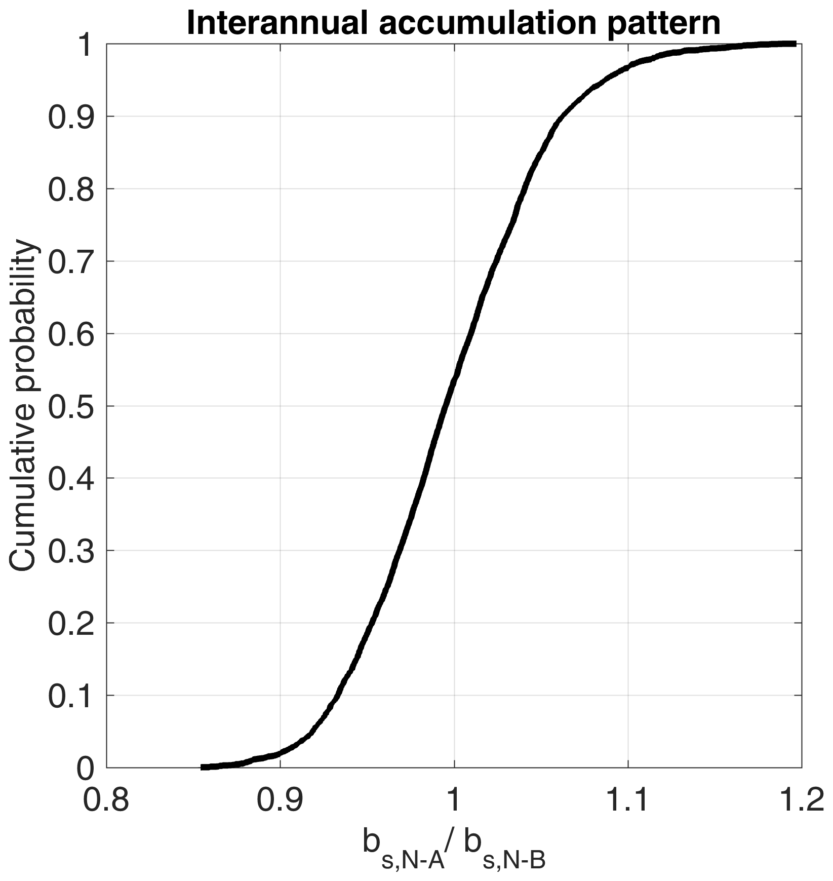
Figure 8 Interannual accumulation pattern comparison for intersecting transects at DYE-2. b_s,N-A corresponds to normalized b_s for winter accumulation 2015/2016 and b_s,N-B to normalized b_s for winter accumulation 2016/2017.

3.4 Temporal changes in accumulation at DYE-2

During snow pit measurements in May 2016, we placed target reflectors at the EMS 2015 surface in each pit. These targets appear as hyperbolas in the radar data and make it possible to unambiguously identify that specific EMS for every subsequent radar campaign. We identified several targets in the May 2017 radar data. Hence, it is possible to detect changes in b_s that occurred between May 2016 (the last radar campaign) and the end of the 2016 melt season (i.e., the start of the 2016/2017 accumulation season). However, such an analysis is only possible for intersecting areas of subsequent radar campaigns, which is 1.7 km² at DYE-2. The area for which both the summer 2015 and summer 2016 IRHs could be clearly identified decreases to 0.76 km². Ice movement contributes to uncertainties as well. Identical locations in May 2016 and May 2017 do not represent identical snow and firn layers, since we observed horizontal ice movement of 25 m at the upGPR location.

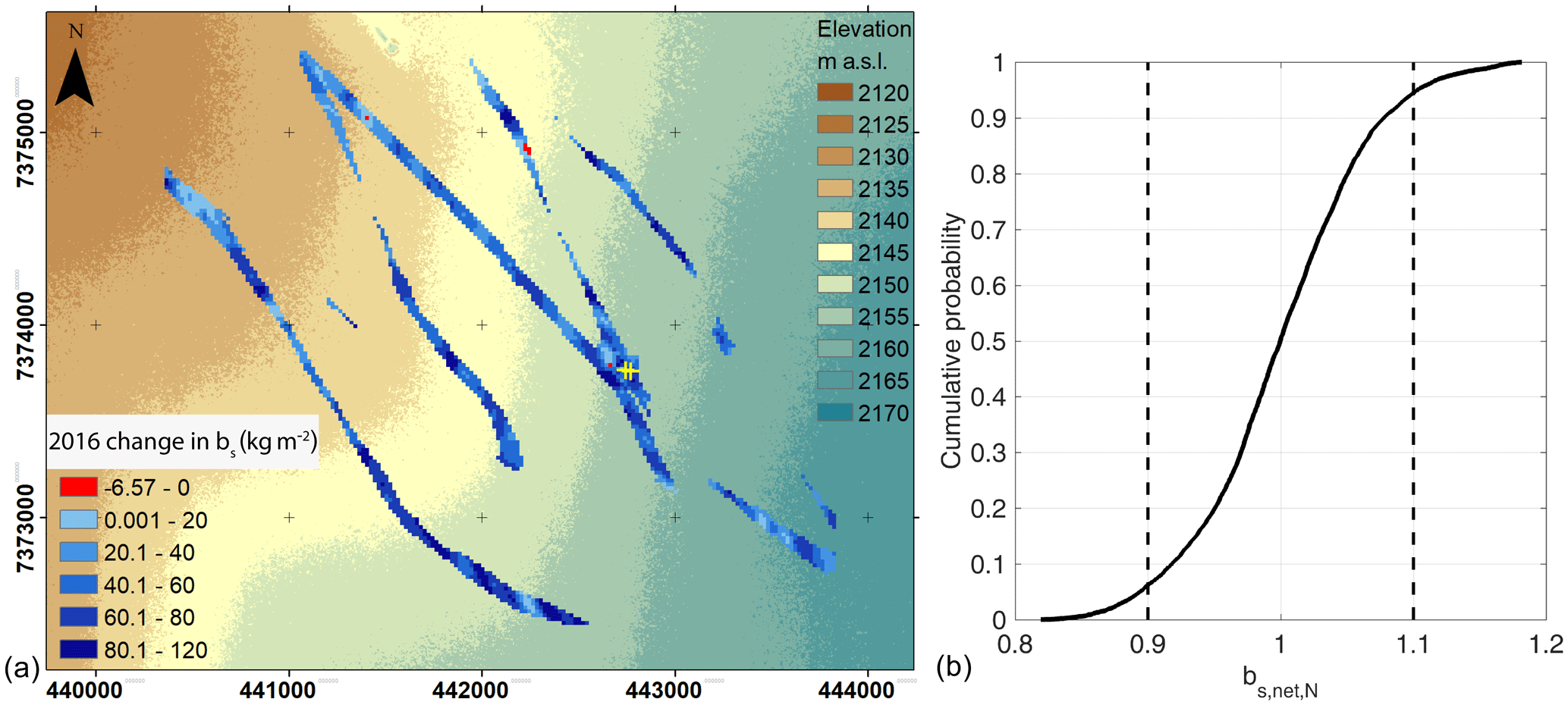
Figure 9 (a) Determined changes in accumulation (b_s) from May 2016 until September 2016. The yellow crosses show locations of the upGPR. The background displays a 2 m digital elevation model (Porter et al., 2018) with 5 m contour color coding starting at 2120 m a.s.l. (brown color) and reaching 2165 m a.s.l. (blue color). The coordinates are given according to UTM with datum WGS 1984. (b) Cumulative probability distribution of the normalized net accumulation ($b_{\mathrm{s},\mathrm{net},\mathrm{N}}$) of the layer between end-of-melt-season 2015 and end-of-melt-season 2016 layers.

Instead of snow pit data, we used a firn core (drilled in May 2017) to determine the density of the layer between the 2015 and 2016 IRHs and to derive accumulation from TWT data as described in Eqs. (1) and (2). The firn between the 2015 IRH and the 2016 IRH is the net accumulation (accumulation minus meltwater percolation) between EMS 2015 and EMS 2016 (b_s,net), whereas the radar data collected in May 2016 are the winter accumulation, from EMS 2015 to May 2016. The changes that occurred over summer 2016, $\mathrm{\Delta }{b}_{\mathrm{s}}=b_{\mathrm{s},\mathrm{net}}-b_{\mathrm{s}}$, are the subtraction of the winter accumulation from the net accumulation for area intersections. The mean $\stackrel{\mathrm{‾}}{\mathrm{\Delta }{b}_{\mathrm{s}}}$ for the intersecting transect areas (Fig. 9a) for summer 2016 is 51 kg m⁻² with a standard deviation of 21 kg m⁻². Figure 9 documents the wide range in the data distribution. The negative values in Fig. 9a occur only for 6 pixels and are likely artifacts.

Data distribution for b_s,net is shown in Fig. 9b as normalized values. Here, the distribution is less narrow than the winter accumulation in May 2016 (Fig. 6d, blue line). Within the uncertainty margins, b_s decreases from p=0.99 to p=0.88 after one summer season. During summer 2016, melt caused a seasonal mass flux of 56 kg m⁻² into firn below EMS 2015 at the upGPR site (Heilig et al., 2018). It is likely that the seasonal mass flux is not homogeneous over the investigated area. In addition, the increased variability is in part due to mismatches in colocating transects due to the ice movement. However, the mean change in b_s during summer 2016 corresponds almost exactly with observations derived from the upGPR (Heilig et al., 2018), which is 50.9 kg m⁻² from 1 May 2016 until the end of the melting period. This may be a coincidence or a confirmation of the benefits of upGPR, which averages a surface area of up to 10 m² compared to 1–3 m² for a snow pit.

We cannot identify trends in b_s associated with elevation over the summer melt in 2016; there are large differences within the same elevation band (Fig. 9a). This implies that (i) no lateral redistribution of mass can be observed at DYE-2 during snow and firn melt and (ii) that melt and seasonal mass fluxes are much more inhomogeneous than accumulation distribution. These conclusions support the assumption made by Heilig et al. (2018) that in the current climate there is no systematic lateral mass redistribution during the melt season at DYE-2.

Table 4 Winter snow accumulation (b_s) and snow density (ρ_s) measured in spring snow pits for DYE-2 and KAN-U compared with determined area-wide arithmetic means.

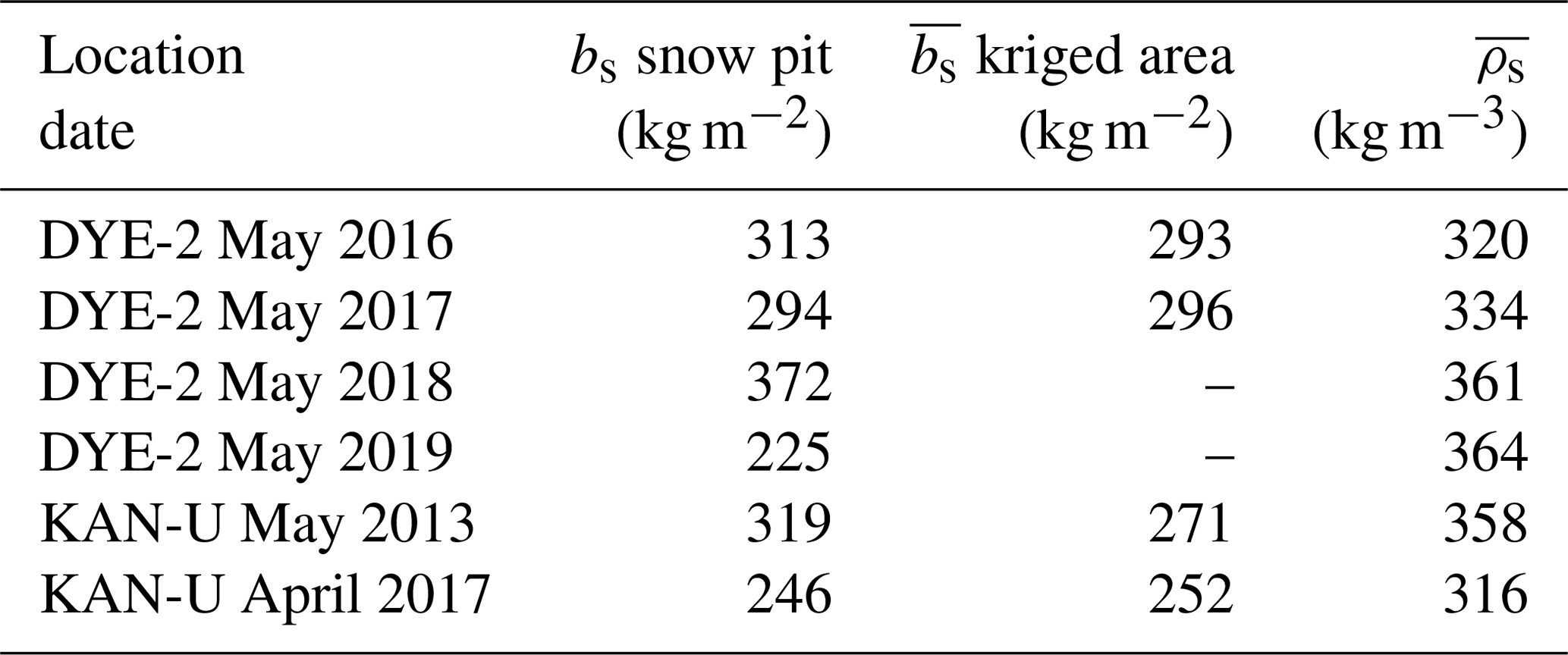
We also measured b_s in snow pits near the upGPR at DYE-2 in May 2018 and 2019. Although accumulation measured in May 2016 and May 2017 was very similar, the 2018 and 2019 data deviate strongly (Table 4). In 2018, b_s was more than 20 % higher than in the previous two accumulation seasons. The accumulation measured in May 2019 was the lowest of the 4 years by a significant margin: 40 % lower than the previous season and 23 % lower than the next-lowest season (2017). This interannual accumulation variability is larger than the ±10 % uncertainty in how well a b_s point measurement can be derived from radar data and usually represents the surrounding area. In agreement with Koenig et al. (2016), we conclude that annual or more frequent density and b_s observations are necessary to estimate mean accumulation rates per region correctly. When snow depth is measured and averaged over an area of roughly 20 m × 20 m, the value provides a reliable estimate of accumulation on regional scales of 1–20 km². Such data can be used for airborne-radar campaigns and for validation of RCM simulations.

4 Conclusions

This study investigated how representative single point observations of b_s, such as snow pits, are for the surrounding 400 m² to 4 km² large areas. We used GPR to track IRHs created by summer melt surfaces along transects at three sites on the southwestern GrIS over the course of several field seasons. We derived maps of snow accumulation variability and compared them to snow pit and upGPR measurements. We found an uncertainty in radar-derived accumulation of 7 %–8 %, which results from neglecting density variations along the radar transect and from applying a smoothing algorithm to minimize surface variability and layer-picking errors. In addition, we investigated the persistence of spatial patterns in accumulation over consecutive years and the influence of melt on an annual firn layer.

At all three sites, we found that point measurements such as snow pits represent the average b_s well over the study areas. A randomly selected snow pit location at any of the three sites would provide b_s values for the surrounding area (i.e., within ±10 % of the areal mean) with a probability of p=0.8 (KAN-U May 2013) to p>0.95 (Swiss Camp May 2015 and DYE-2 May 2016). These likelihoods are independent of the size of the investigated areas. However, not measuring and averaging snow depth over an area of at least 20 m × 20 m decreases the probability of hitting arithmetic means by at least 10 %. Snow density variability is usually below ±5 % on regional scales (1–4 km²), while snow depth can vary significantly because of surface features such as dunes and sastrugi with various wavelengths ranging from submeters up to 60 m and more.

Our results suggest that there is only little change in accumulation patterns at DYE-2 for spring 2016 and 2017. However, the data only span two consecutive accumulation seasons that were almost identical in average density and accumulation. As such, we cannot confirm whether such persistence might be observed in seasons with significantly more or less accumulation or at different sites; this is a topic for future work.

We also investigated the mass change that an accumulation layer (end-of-melt season to May) undergoes during the summer melt season using the GPR transect data and continuous melt and accumulation observations from upGPR. We conclude that temporal changes in firn layer mass detected by the upGPR are representative of larger (∼1 km²) areas at DYE-2. We did not detect any patterns in summer melt along flow lines, suggesting that lateral meltwater flow at DYE-2 is not significantly redistributing mass. However, this could change with future warming in Greenland, which would significantly influence data interpretation of point measurements (AWS data, snow pits) and regional predictions by RCM and remote sensing.

This study aims to close the gap between point observations of b_s, which are meter scale, and remote-sensing data and RCMs, which have pixel sizes of ∼1–20 km. We have shown that snow accumulation in the regions surrounding the three sites of the southwestern GrIS can be estimated well by point measurements as long as the snow depth is not influenced by surface roughness. To minimize such roughness effects, it is essential to determine the average snow depth over an area of several square meters. Ideally, snow depth determinations – either directly via probings or derived from GPR transects – comprise spacings between single points smaller than the characteristic length of the features and have an extent larger than the wavelengths of the features. Our analyses suggest that snow density does not vary greatly over kilometer scales, and as such a single density measurement with numerous probed depths can suffice. Because interannual variability in accumulation can be significant, field measurements are essential for validating RCM predictions and remote-sensing products.

Appendix A

Figure A1 Prevailing wind distribution at Swiss Camp (a), DYE-2 (b) and KAN-U (c).