The firn meltwater Retention Model Intercomparison Project (RetMIP): evaluation of nine firn models at four weather station sites on the Greenland ice sheet

Perennial snow, or firn, covers 80 % of the Greenland ice sheet and has the capacity to retain surface meltwater, influencing the ice sheet mass balance and contribution to sea-level rise. Multilayer firn models are traditionally used to simulate firn processes and estimate meltwater retention. We present, intercompare and evaluate outputs from nine firn models at four sites that represent the ice sheet's dry snow, percolation, ice slab and firn aquifer areas. The models are forced by mass and energy fluxes derived from automatic weather stations and compared to firn density, temperature and meltwater percolation depth observations. Models agree relatively well at the dry-snow site while elsewhere their meltwater infiltration schemes lead to marked differences in simulated firn characteristics. Models accounting for deep meltwater percolation overestimate percolation depth and firn temperature at the percolation and ice slab sites but accurately simulate recharge of the firn aquifer. Models using Darcy's law and bucket schemes compare favorably to observed firn temperature and meltwater percolation depth at the percolation site, but only the Darcy models accurately simulate firn temperature and percolation at the ice slab site. Despite good performance at certain locations, no single model currently simulates meltwater infiltration adequately at all sites. The model spread in estimated meltwater retention and runoff increases with increasing meltwater input. The highest runoff was calculated at the KAN_U site in 2012, when average total runoff across models (±2σ) was 353±610 mm w.e. (water equivalent), about 27±48 % of the surface meltwater input. We identify potential causes for the model spread and the mismatch with observations and provide recommendations for future model development and firn investigation.

1 Introduction

In response to higher air temperatures and increased surface melt, the Greenland ice sheet has been losing mass at an accelerating rate over recent decades and is responsible for about 20 % of observed global sea-level rise (Van den Broeke et al., 2016; IMBIE Team, 2020). Increasing temperatures have introduced melt at higher elevations where it was previously seldom observed (Nghiem et al., 2012). In these colder, elevated areas, snow builds up into a thick layer of firn. Increased surface melt in the firn area of the Greenland ice sheet affects the firn structure (Machguth et al., 2016; Mikkelsen et al., 2016), density (de la Peña et al., 2015; Vandecrux et al., 2018), air content (van Angelen et al., 2013; Vandecrux et al., 2019) and temperature (Polashenski et al., 2014; Van den Broeke et al., 2016). These changing characteristics impact the firn's meltwater storage capacity, through its ability to either refreeze meltwater (Pfeffer et al., 1991; Braithwaite et al., 1994; Harper et al., 2012) or retain liquid water in perennial firn aquifers (e.g., Forster et al., 2014; Miège et al., 2016). Meltwater refreezing can for instance form continuous ice layers that are several meters thick (MacFerrin et al., 2019). These ice slabs impede vertical meltwater percolation, enhance surface water runoff (Machguth et al., 2016; Mikkelsen et al., 2016; MacFerrin et al., 2019) and lower the surface albedo (Charalampidis et al., 2015), further amplifying Greenland's contribution to sea-level rise. The evolution of firn on the Greenland ice sheet is important for two additional reasons. First, knowledge about how firn air content evolves through time is necessary for the conversion of space-borne observations of ice sheet volume change into mass change (e.g., Sørensen et al., 2011; Zwally et al., 2011). Secondly, the depth of firn-to-ice transition as well as the mobility of gases through the firn before they are trapped in bubbles within glacial ice is necessary for the interpretation of ice cores and heavily depends on the fine coupling between the firn characteristics and surface conditions (e.g., Schwander et al., 1993).

Snow and firn models have been traditionally used to calculate the evolution of firn characteristics and meltwater retention at scales ranging from tens of meters to tens of kilometers. The performance of these models, when coupled to regional and global climate models, has a direct impact on the fidelity of ice sheet mass balance calculations (Fettweis et al., 2020) and sea-level change estimations (Nowicki et al., 2016). In previous work, Reijmer at al. (2012) suggested that, provided reasonable tuning, simple parameterizations of the subsurface processes calculate refreezing rates for the Greenland ice sheet in agreement with results from physically based, multilayer firn models. However, spatial patterns varied widely, and evaluation against field observations remained challenging. Steger et al. (2017) and more recently Verjans et al. (2019) investigated the impact of meltwater infiltration schemes on the simulated properties of the firn in Greenland. These studies highlighted the potential of deep-percolation schemes, for instance for the simulation of firn aquifers but also the sensitivity of simulated infiltration to the firn structure and hydraulic properties. In these previous studies, the surface conditions were prescribed by a regional climate model. Inaccuracies in this forcing could therefore explain some of the deviation between model outputs and firn observations and prevented a full assessment of different firn model designs.

The meltwater Retention Model Intercomparison Project (RetMIP) compares results from nine firn models currently used for the Greenland ice sheet. The models are forced with consistent surface inputs of mass and energy, and simulations are performed at four sites where surface conditions could be derived from automatic weather station (AWS) observations and where firn observations are available. These four sites were chosen to represent various climatic zones of the Greenland ice sheet firn area: the dry-snow area, where melt is rare, and temperatures are low, is represented by Summit; the percolation area, where melt occurs every summer at the surface, infiltrates in the snow and firn and refreezes there, is represented by Dye-2; ice slab regions, where a thick ice layer hinders deep meltwater percolation, is represented by KAN_U; and firn aquifer regions, where infiltrated meltwater remains liquid at depth, is represented by FA. At each site, we compare simulated temperatures, densities and the resulting meltwater infiltration patterns between models and to in situ measurements. We discuss model features that can be responsible for the model spread and deviations from observations. Lastly, we evaluate how differences in simulated firn characteristics result in various simulated refreezing and runoff values at Dye-2 and KAN_U and attempt to quantify uncertainties linked to firn models.

Table 1 Models evaluated in this study.

2 Models

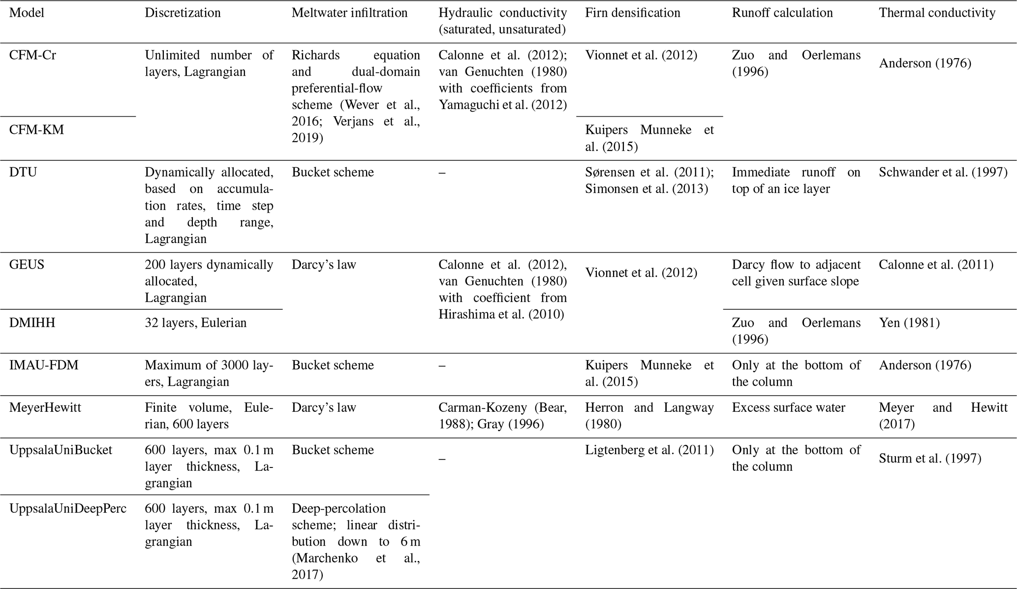
The multilayer firn models investigated here are listed in Table 1. They all have density, temperature and liquid water content as prognostic variables and apply a framework whereby firn is divided into multiple layers for which these characteristics can be calculated. The number of layers varies in each model (Table 2), and we distinguish between two distinct types of layer management strategies: all models except DMIHH and MeyerHewitt follow a Lagrangian framework; i.e., they add new layers at the top of the model column during snowfall, and these layers are advected downward as new material accumulates at the surface. DMIHH and MeyerHewitt follow an Eulerian framework in which the layers have either fixed mass or fixed volumes. During snowfall, new material is added to the first layer, and an equivalent mass or volume is transferred by each layer to its underlying neighbor. At each time step, the models calculate firn density according to different densification formulations and update the layer temperature using different values of thermal conductivity (Table 2). The DMIHH, GEUS and DTU models have a fixed temperature at the bottom of their column (Dirichlet boundary condition), while other models have a fixed temperature gradient (Neuman boundary condition).

All models simulate meltwater percolation and transfer water vertically from one layer to the next according to the routines listed in Table 2. They also simulate meltwater refreezing and latent-heat release. All models simulate the retention of meltwater within a layer due to capillary suction, either explicitly (MeyerHewitt, CFM-Cr and CFM-KM) or, for all the other models, parameterized through the use of an irreducible water content (Coléou and Lesaffre, 1998; Schneider and Jansson, 2004). When meltwater cannot be transferred to the next layer or be retained within the layer by capillary suction, lateral runoff can occur according to model-specific rules (Table 2). The background and specifics of each model are described in greater detail in the following paragraphs.

2.1 CFM-Cr and CFM-KM models

The Community Firn Model (CFM) is an open-source, modular model framework designed to simulate a range of physical processes in firn (Stevens et al., 2020). The number of layers for a particular model run is fixed and determined by the accumulation rate and time step size. New snow accumulation at each time step is added as a new layer, and a layer is removed from the bottom of the model domain. A layer-merging routine prevents the number of layers from becoming too large. CFM-Cr and CFM-KM use the Crocus (Vionnet et al., 2012) and Kuipers Munneke et al. (2015) densification schemes, respectively (Table 2). Both use the same meltwater percolation scheme: a dual-domain approach that closely follows the implementation of the SNOWPACK snow model (Wever et al., 2016). It accounts for the duality of water flow in firn by simulating both slow matrix flow and fast, localized, preferential flow (Verjans et al., 2019). In the matrix flow domain, water percolation is prescribed by the Richards equation; ice layers are impermeable, and runoff is allowed. In contrast, water in the preferential-flow domain is allowed to bypass such barriers but not to run off. Water is exchanged between both domains as a function of the firn layer properties: density, temperature and grain size. As such, when water in the matrix flow domain accumulates above an ice layer, it is progressively depleted by runoff and by transfer of water into the preferential-flow domain. In the deepest firn layers, above the impermeable ice sheet, water accumulates, and no runoff is prescribed, which allows for the buildup of firn aquifers.

2.2 DTU model

The DTU firn model was developed to derive the Greenland ice sheet mass balance from the satellite observations of ice sheet elevation change (Sørensen et al., 2011) and to describe the firn stratigraphy and annual layers in the dry-snow zone along the EGIG line in central Greenland (Simonsen et al., 2013). The DTU model uses the densification scheme from Arthern et al. (2010) and a bucket scheme for meltwater infiltration and retention. If meltwater is conveyed to a model layer, the water is refrozen if sufficient pore space and cold content are available in the layer. Additional liquid water can be retained in a layer by capillary forces calculated after Schneider and Jansson (2004). This formulation does not allow for the formation of firn aquifers. Percolation continues until the water encounters a layer at ice density or the bottom of the model, where, in both cases, it is assumed to run off. The model follows a Lagrangian scheme of advection of layers down into the firn, and the model layering is defined by the time-stepping of the model.

2.3 DMIHH model

The DMIHH model was developed to provide firn subsurface details for the HIRHAM regional climate model experiments (Langen et al., 2017). DMIHH employs 32 layers, within which snow, ice and liquid water fractions can vary and where each layer has a constant mass. Layer thicknesses increase with depth to increase resolution near the surface and give a full model depth of 60 m water equivalent (w.e.). Mass added at the surface (e.g., snowfall) or removed as runoff causes the scheme to advect mass downward or upward to ensure the constant w.e. layer thicknesses. DMIHH uses Darcy's law to describe meltwater infiltration. In addition to the saturated and unsaturated hydraulic conductivities (Table 2), the water flow through layers containing ice follows the model of Colbeck (1975) for a snowpack with discontinuous ice layers. A parameter describing the ratio between the characteristic distance between two adjacent ice lenses and the characteristic width of an ice lens was set to 1, meaning that ice lenses have a horizontal extent of half the unit area. A layer is considered impermeable if its bulk dry density exceeds 810 kg m⁻³. Runoff is calculated from the water in excess of the irreducible saturation with a characteristic local runoff timescale that increases as the surface slope tends to 0, following the parameterization from Zuo and Oerlemans (1996) with the coefficients from Lefebre et al. (2003). DMIHH has an initial value of 0.1 mm for the grain diameter of freshly fallen snow. The column grain size distribution is initialized in these experiments as columns taken at the specific sites from the spin-up experiments performed by Langen et al. (2017).

2.4 GEUS model

The GEUS model is based on the DMIHH model (Langen et al., 2017) and is further developed in Vandecrux et al. (2018, 2020a). The main differences from DMIHH are the Lagrangian management of model layers and the increased vertical resolution with 200 layers. As in the DMIHH model, the layer's ice content decreases its hydraulic conductivity according to Colbeck (1975), but the ice layer geometry parameter was set to 0.1 as detailed in Vandecrux et al. (2018). Water exceeding the irreducible water content that could not percolate downward is available for runoff and is removed from the layer at a rate that depends on the firn characteristics and on surface slope, according to Darcy's law. More details about this runoff scheme are provided in the Supplement Text S1.

2.5 IMAU-FDM

The IMAU-FDM model has been used in combination with the RACMO regional climate model in Greenland, Arctic Canadian ice caps and Antarctica. Firn compaction follows a semiempirical, temperature-based equation from Arthern (2010). The compaction rate is tuned to observations from Greenland firn cores using an accumulation-based correction factor (Kuipers Munneke et al., 2015). IMAU-FDM includes meltwater percolation following a bucket approach. Percolating meltwater is refrozen if there is space available in the layer and if the latent heat of refreezing can be released in the layer. As opposed to other models in this study, runoff is not allowed over ice layers but only when percolating meltwater has reached the pore close-off depth. Upon reaching that depth, runoff is instantaneous. The rationale for allowing percolation through thick ice slabs is that IMAU-FDM is mainly used to simulate firn at scales of tens to hundreds of square kilometers, and at these spatial scales, meltwater is assumed to always find a way through even the thickest of ice slabs.

2.6 MeyerHewitt model

Meyer and Hewitt (2017) present a continuum model for meltwater percolation in compacting snow and firn. The MeyerHewitt model includes heat conduction, meltwater percolation and refreezing as well as mechanical compaction using the empirical Herron and Langway (1980) model. In the MeyerHewitt model, water percolation is described using Darcy's law, allowing for both partially and fully saturated pore space. Water is allowed to run off from the surface if the snow is fully saturated. Using an enthalpy formulation for the problem, the MeyerHewitt model is discretized using an Eulerian, conservative finite-volume method that is fixed to the surface.

Table 2 Model characteristics.

2.7 UppsalaUniBucket and UppsalaUniDeepPerc models

UppsalaUniBucket and UppsalaUniDeepPerc have been developed for the Norwegian Arctic (Van Pelt et al., 2012, 2019; Marchenko et al., 2017) and only differ in their representation of vertical water transport. UppsalaUniBucket simulates meltwater percolation according to a bucket scheme, while UppsalaUniDeepPerc uses a deep-percolation scheme which mimics the effect of fast vertical transport due to preferential flow (Marchenko et al., 2017). This deep-percolation scheme acts before the bucket scheme and instantaneously transfers the meltwater available at the surface to underlying layers using a linear distribution function of depth that reaches 0 at 6 m depth (Marchenko et al., 2017). The water transport model incorporates irreducible water storage and allows infiltration through ice-dominated layers. All water that reaches the base of the firn column is set to run off instantaneously. References for the parameterizations used for gravitational settling, thermal conductivity, irreducible water storage and water percolation are given in Table 2.

3 Methods

3.1 Site selection and surface forcing

Differences between firn model outputs and observations depend on the model formulation but also on the forcing data that are given to the model: any bias in forcing data propagates into the model output. To make sure we compare and evaluate the models independently of biases that may exist in forcing datasets that come from regional climate models, we use meteorological fields derived from five AWSs at four sites.

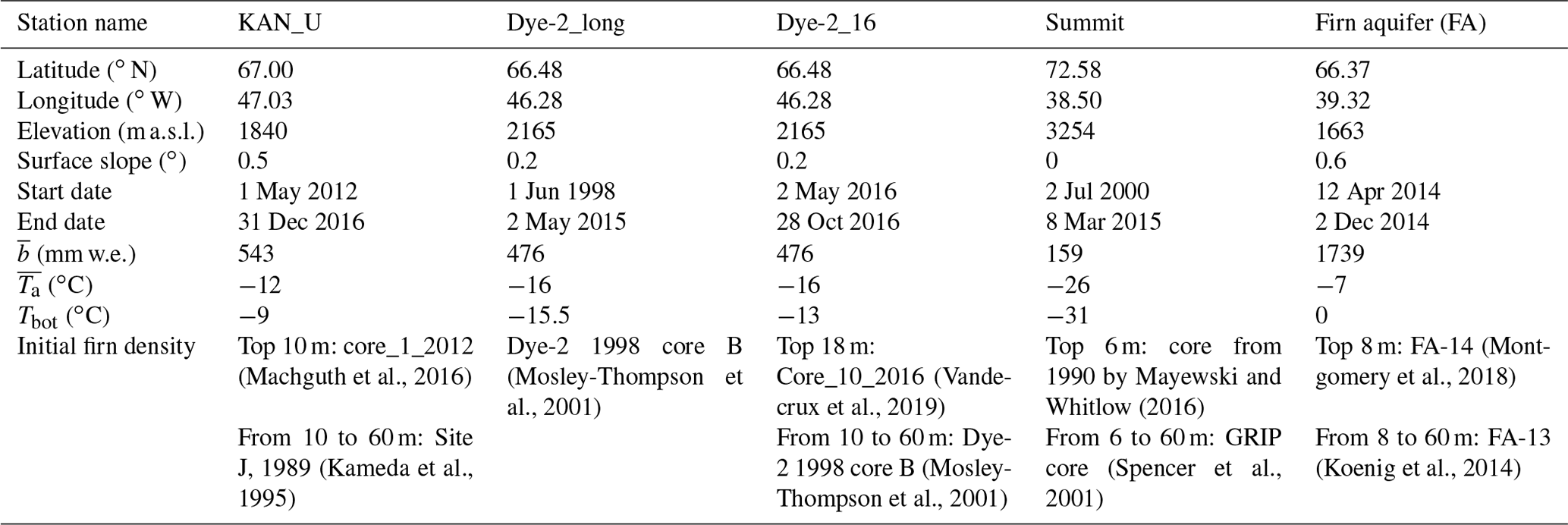
These sites represent a broad range of climatic conditions on the Greenland ice sheet (Table 3, Fig. 1) that produce a wide variety of firn density and temperature profiles. For example, the cold and dry climate at the Summit station produces cold firn with low compaction rates representative of the “dry snow” area as defined by Benson (1962). Dye-2, located in an area with higher melt (Table 3), is representative of the “percolation area” (Benson, 1962), where meltwater generated at the surface percolates into the firn and releases latent heat when refreezing into ice lenses. At the KAN_U site, lower accumulation rates and increasing melt have led to the formation of thick ice slabs (Machguth et al., 2016; MacFerrin et al., 2019) that impede meltwater percolation below 5 m. The firn aquifer (FA) site in southeastern Greenland has both high surface melt and high accumulation rate, leading to the formation of a perennial body of liquid water at a depth of 12 m and below (Forster et al., 2014; Kuipers Munneke et al., 2014).

We use data from the Greenland Climate Network (GC-Net) AWS at Dye-2 and Summit (Steffen et al., 1996) and from the Programme for Monitoring of the Greenland Ice Sheet (PROMICE) station at KAN_U (Ahlstrøm et al., 2008; Charalampidis et al., 2015). For Dye-2 in 2016, we use an AWS installed by the University of Calgary and described in Samimi et al. (2020). Since this station was more recently installed than the GC-Net station, it ensures better meteorological observations (leveling, absence of frost or mist on radiometers) and therefore better forcing for the models over the 2016 melting season, during which an extensive observational dataset is available for model evaluation. This simulation is henceforth referred to as Dye-2_16, while the longer simulation using the GC-Net AWS is referred to as Dye-2_long. At FA, we use data from the S21 AWS maintained by Utrecht University. The S21 AWS measures air temperature, relative humidity (Vaisala HMP35AC), air pressure (Vaisala PTB101B), wind speed and direction (Young 05103), the shortwave and longwave radiative fluxes (Kipp and Zonen CNR1), station tilt, and instrument height. All quantities are sampled every 6 min, and hourly averages are recorded by a Campbell CR10X data logger.

Data from each AWS were quality-checked, and obvious sensor malfunctions were discarded. No data were discarded at FA and Dye-2_16. Gaps in the temperature, wind speed, humidity, air pressure, and incoming shortwave and longwave radiation were filled with adjusted values from either nearby stations or HIRHAM5, following Vandecrux et al. (2018). Gaps in upward shortwave radiation were filled using gap-filled downward shortwave radiation and the nearest daily albedo values from the Moderate Resolution Imaging Spectroradiometer (MODIS) satellite (Box et al., 2017). Downward longwave radiation is not monitored by the GC-Net stations (Dye-2_long and Summit) and is taken entirely from HIRHAM5 output.

The gap-filled meteorological fields are used to calculate the surface energy balance based on the model developed by van As et al. (2005) and applied in Vandecrux et al. (2018). We use surface height measurements and available snow pit information to calculate snowfall rates as in Vandecrux et al. (2018). This surface energy and mass balance provides, at 3-hourly resolution, the three surface forcing fields that were used by all models: the surface skin temperature, the amount of meltwater generated at the surface, and net snow accumulation (snowfall − sublimation + deposition). Only the MeyerHewitt model required minor adaptation of these forcing fields (see Supplement Text S1). Rain is not monitored at any site, so it is not included in the mass fluxes. Tilt of the radiation sensor was not corrected for at Dye-2_long and Summit stations although this correction was seen to increase the calculated melt by 35 mm w.e. yr⁻¹ at Dye-2 (Vandecrux et al., 2020a). The surface forcing data are illustrated in Fig. S3.

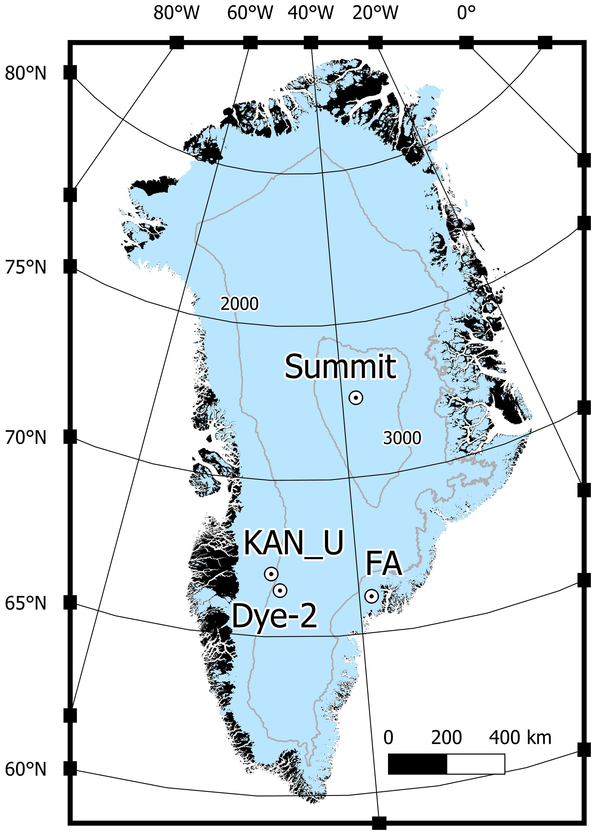
Figure 1 Map of the four study sites. Elevation contours are in meters above sea level.

Table 3 Information about the four sites and five model runs considered in the comparison, including mean annual accumulation ($\stackrel{\mathrm{‾}}{b}$), mean annual air temperature ($\stackrel{\mathrm{‾}}{T_{\mathrm{a}}}$) and prescribed bottom firn temperature (T_bot).

3.2 Boundary conditions

To allow fair comparison, all models shared as many boundary conditions as possible. A key parameter in firn models is the density of fresh snow added at the top of the model column. Here, all models used the value of 315 kg m⁻³ from Fausto et al. (2018), which is derived from a compilation of 200 top 10 cm snow density observations from the Greenland ice sheet. Initial profiles for density, temperature and liquid water content (only at FA) were provided to all models and are illustrated in Fig. S4 in the Supplement. The references for the initial density profiles are given in Table 3. Initial temperature profiles were calculated using the first reading of air temperature (as first guess of surface temperature), the first valid measurement of firn temperature and the bottom firn temperature (Table 3). The bottom firn temperatures (Table 3), needed as a lower boundary condition by some of the models, were calculated from the available firn temperature measurements. At KAN_U, the average of the deepest firn temperature, at ∼8 m depth, was taken over the spring 2013–spring 2015 period. At Summit and Dye-2_long, the 10 m firn temperature was interpolated when firn temperature measurements were below 10 m depth and then averaged. For Dye-2_16 and FA, the deepest firn temperature measurement, at 9 and 25 m depth respectively, were averaged over their respective measurement periods (Table 3). Initial liquid water content at FA is calculated according to the observations from Koenig et al. (2014), which indicate pore saturation below 12.2 m depth. Some models also need long-term mean air temperature and accumulation (Table 3), which were calculated from Box (2013) and Box et al. (2013).

3.3 Intercomparison and evaluation of model outputs

Participating models provided simulated firn density, temperature and liquid water content at 3-hourly time steps, interpolated to a common 10 cm grid from the surface to 20 m depth. Additionally, 3-hourly vertically integrated refreezing and runoff were calculated by each model.

Three types of datasets are available at our sites for model evaluation: (i) firn temperature observations from AWS as presented by Vandecrux et al. (2020a) at Summit and Dye-2_long, Heilig et al. (2018) at Dye-2_16 , Charalampidis et al. (2015) at KAN_U and Koenig et al. (2014) at FA; (ii) firn density profiles (Table 4); and (iii) observations of meltwater infiltration depth at Dye-2 from an upward-looking ground-penetrating radar (upGPR) during summer 2016 (Heilig et al., 2018).

Table 4 Firn cores used for model evaluation.

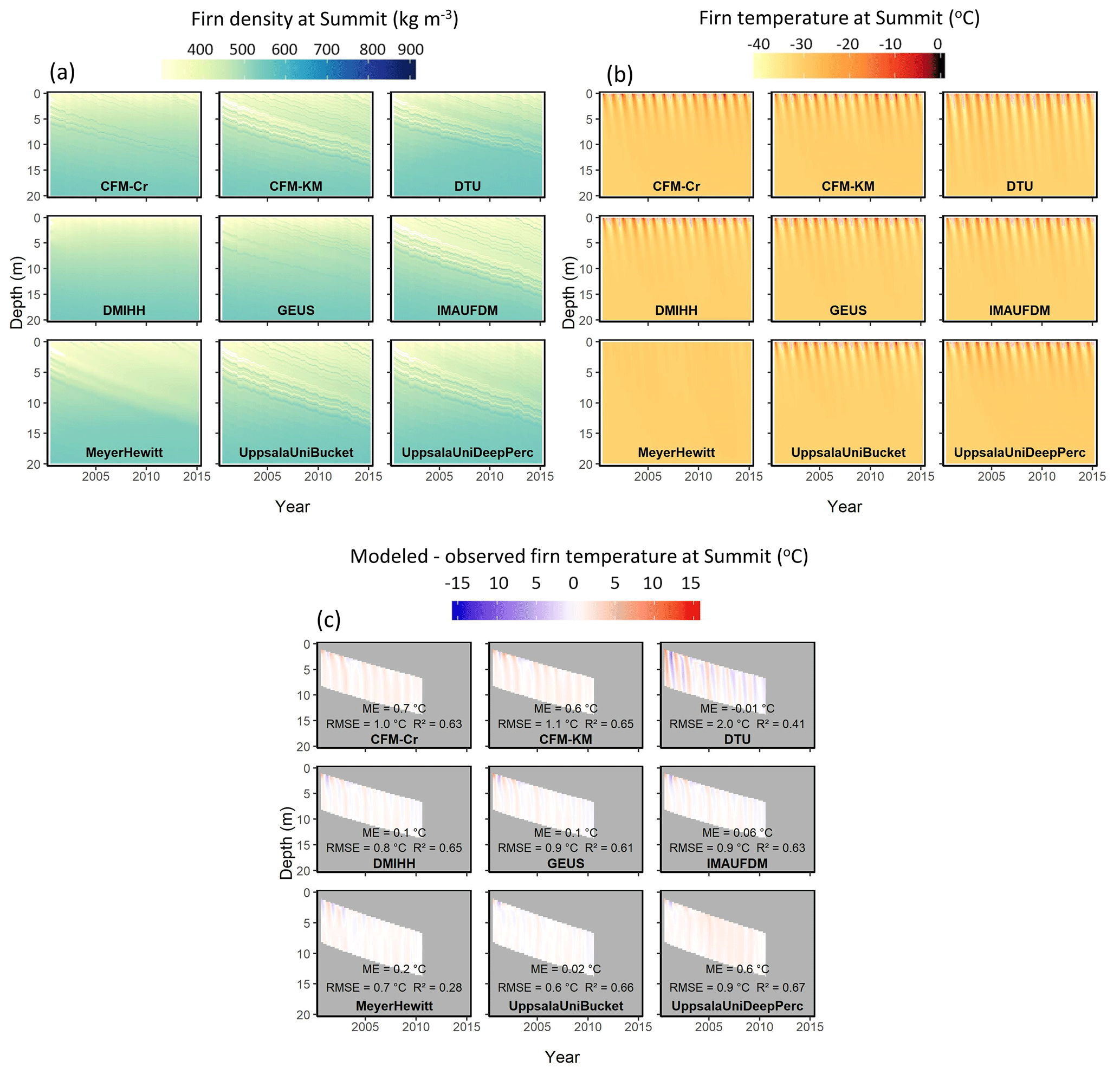
Figure 2 Simulated firn density (a), temperature (b) and deviation between simulated and observed firn temperature (c) at Summit.

For firn density, we calculate for each time step the average firn density over the 0–1, 1–10 and 10–20 m depth ranges and discuss the standard deviation of these values among models and their deviation from firn core observations. We also compare the simulated density profiles to the firn core data at each site. For firn temperature, we compare hourly observations of firn temperature to interpolated temperature from the closest model layers and use the mean error (ME), root mean square error (RMSE) and coefficient of determination (R²) to quantify the performance of the models with respect to the observations.

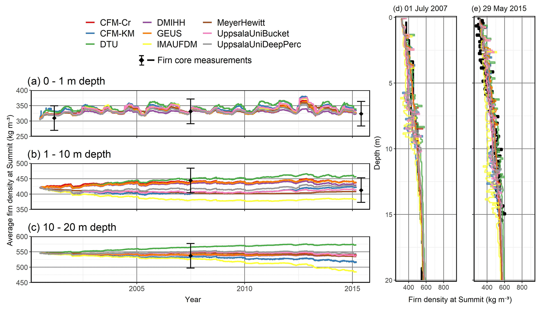
Figure 3 Modeled (colored lines) and observed (black diamonds with ±40 kg m⁻³ uncertainty bars) average firn density for the 0–1 m (a), 1–10 m (b) and 10–20 m depth range (c) at Summit. Note the different density scales. Comparison of simulated and observed firn density profiles (d, e). In (e) the last modeled density profiles, from 8 March 2015, are compared to an observation from 29 May 2015.

4 Results

In the following, we present comparisons of firn model outputs and model deviations from observations for firn temperature, density and liquid water content at sites representing different firn and meltwater regimes: dry firn (Summit), the percolation zone (Dye-2), ice slabs (KAN_U), and a firn aquifer (FA).

4.1 Dry-firn site: Summit

At Summit, density evolves in a similar manner across all models: low-density snow is deposited at the surface and is advected to greater depth (Fig. 2a). All models except DMIHH and MeyerHewitt preserve and advect downward the initial density profile and generate layered firn at the surface. The temporal evolution of the average density for the 0–1 m depth range follows similar seasonality and slight increasing trend (Fig. 3a). Over the 1–10 and 10–20 m depth (Fig. 3b, c), most models produce increasing firn density apart from IMAU-FDM, in which the firn density slightly decreases. All models agree relatively well on the average density independent of the depth range, with a maximum standard deviation among models of 15 kg m⁻³ for the top 1 m average density (of 336 kg m⁻³), 27 kg m⁻³ for the 1–10 m range (420 kg m⁻³ on average) and 23 kg m⁻³ for the 10–20 m range (542 kg m⁻³ on average) during the 15-year-long simulation period (Fig. 3). In comparison with the firn cores drilled in 2007 and 2015, most models reproduce vertical variability in firn density within observation uncertainties (Fig. 3d, e). The evaluation of the density profiles reveals that IMAU-FDM underestimates firn density between 5 and 15 m depth.

Regarding firn temperature, in most models, seasonal skin temperature fluctuations drive firn temperature variability in the top few meters of the column. However, seasonal temperature fluctuations propagate much deeper in the DTU model, while it is almost not visible in the MeyerHewitt model (Fig. 2b). This results in much lower R² when comparing these two models to firn temperature observation: 0.41 and 0.28 for DTU and MeyerHewitt respectively. This results from the numerical strategy and/or thermal diffusivity used in these models. Models that have explicit formulation for deep meltwater infiltration (CFM-Cr, CFM-KM and UppsalaUniDeepPerc) have a positive ME of 0.6 to 0.7 ^∘C. This is due to the simulation of short-lived deep-percolation events that infiltrate the minor melt from the surface down to ∼5 m and to the subsequent refreezing and latent-heat release. DMIHH, GEUS, IMAU-FDM and UppsalaUniBucket provide the lowest ME compared to firn temperature observations (Fig. 2c). Yet, it should be noted that IMAU-FDM calculates adequate heat diffusion while underestimating the firn density (Fig. 3e). Either the firn density underestimation in IMAU-FDM is not sufficient to induce a noticeable change in thermal conductivity or the thermal conductivity and/or numerical scheme used by IMAU-FDM compensate for the underestimated density and result in adequate simulated firn temperature.

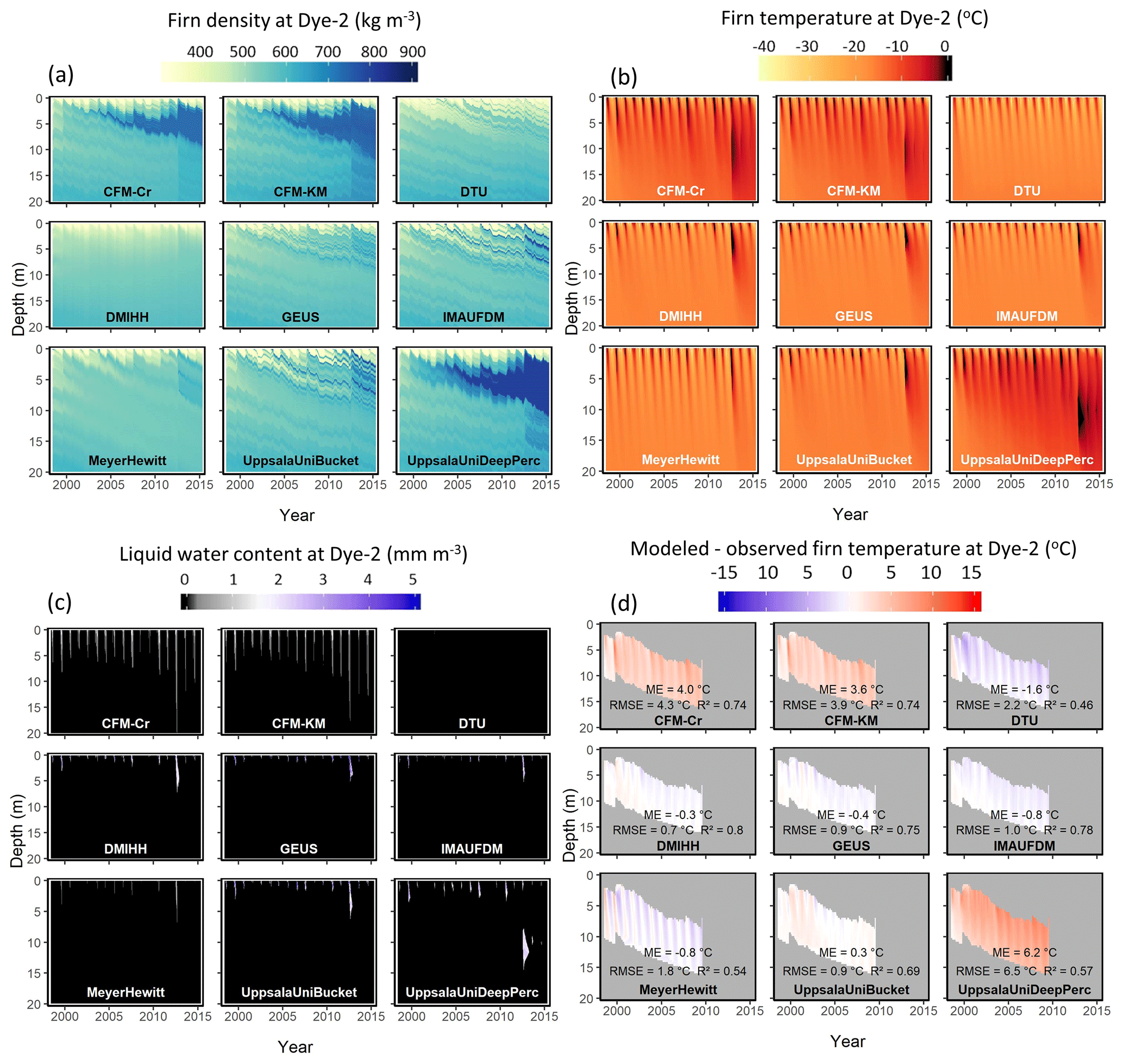
Figure 4 Simulated firn density (a), temperature (b), water content (c) and deviation between simulated and observed firn temperature (d) at Dye-2_long.

Figure 5 Modeled (colored lines) and observed (black diamonds with 40 kg m⁻³ uncertainty bars) average firn density for the top 1 m (a), the 1–10 m depth range (b) and the 10–20 m depth range (c) at Dye-2_long. Observed and simulated firn density profiles at Dye-2_long (d–f).

4.2 Percolation site: Dye-2

At Dye-2, surface melt occurs every summer. Consequently, refreezing of percolating meltwater has a significant effect on simulated density and temperature (Fig. 4). The investigated models span a large spectrum of meltwater infiltration strategies (Table 2), leading to greater differences between models in firn density, temperature and liquid water content (Fig. 4). Simulated meltwater percolation depth varies greatly among the models (Fig. 4c). At one end of the spectrum, the DTU model only allows meltwater in the top model layer: an ice layer is built right at the start of the simulation, and water is not able to penetrate ice layers in this model. At the other end, CFM-Cr and CFM-KM, which do allow meltwater to pass through ice layers and explicitly account for fast preferential flow, simulate percolation down to 10 m depth. In between these end-member models, UppsalaUniDeepPerc simulates percolation down to ∼5 m depth. IMAU-FDM, UppsalaUniBucket, DMIHH and GEUS models give similar results and percolate water down to 1–3 m.

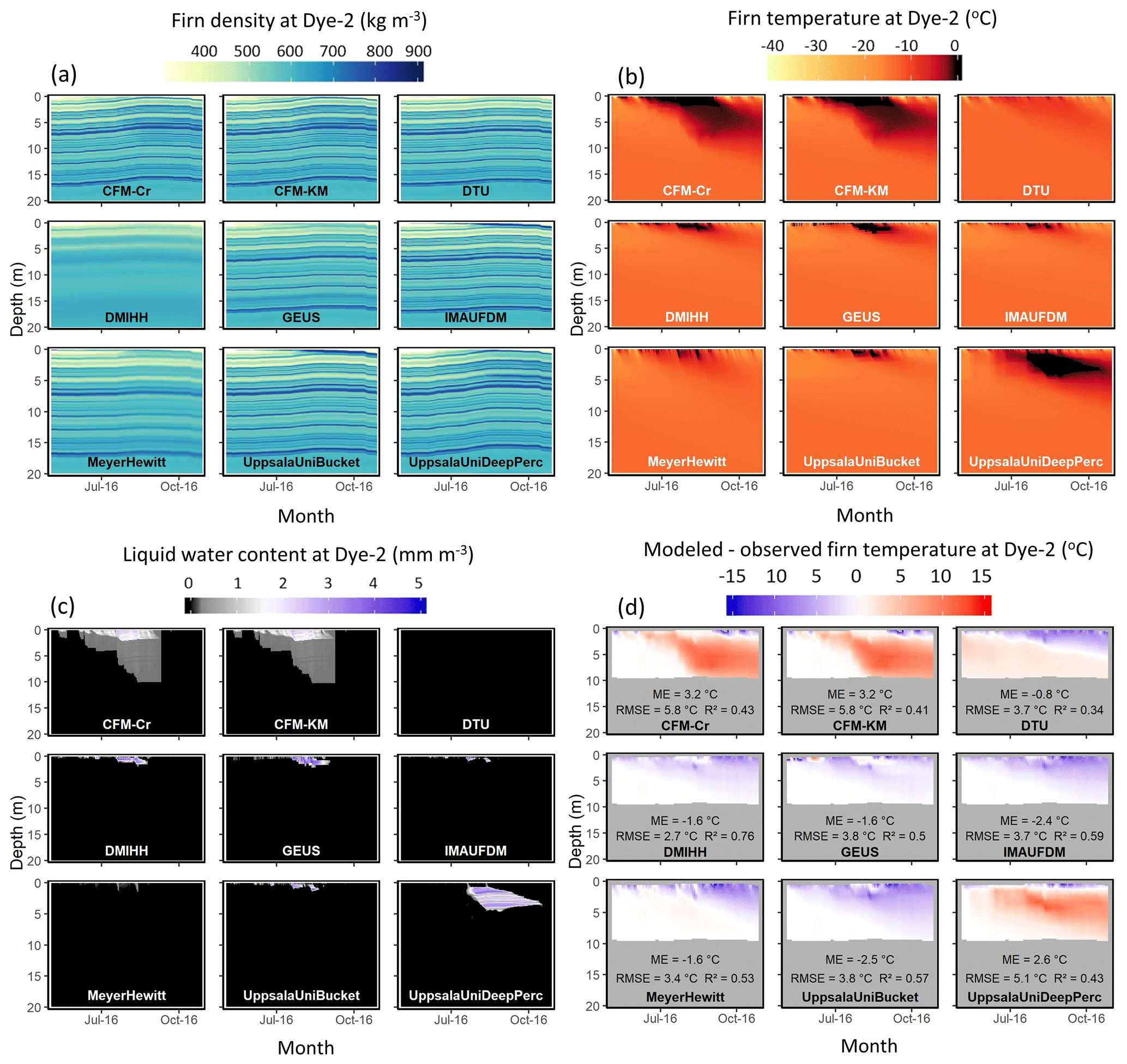
Figure 6 Simulated firn density (a), temperature (b), water content (c), and deviation between simulated and observed firn temperature (d) at Dye-2_16.

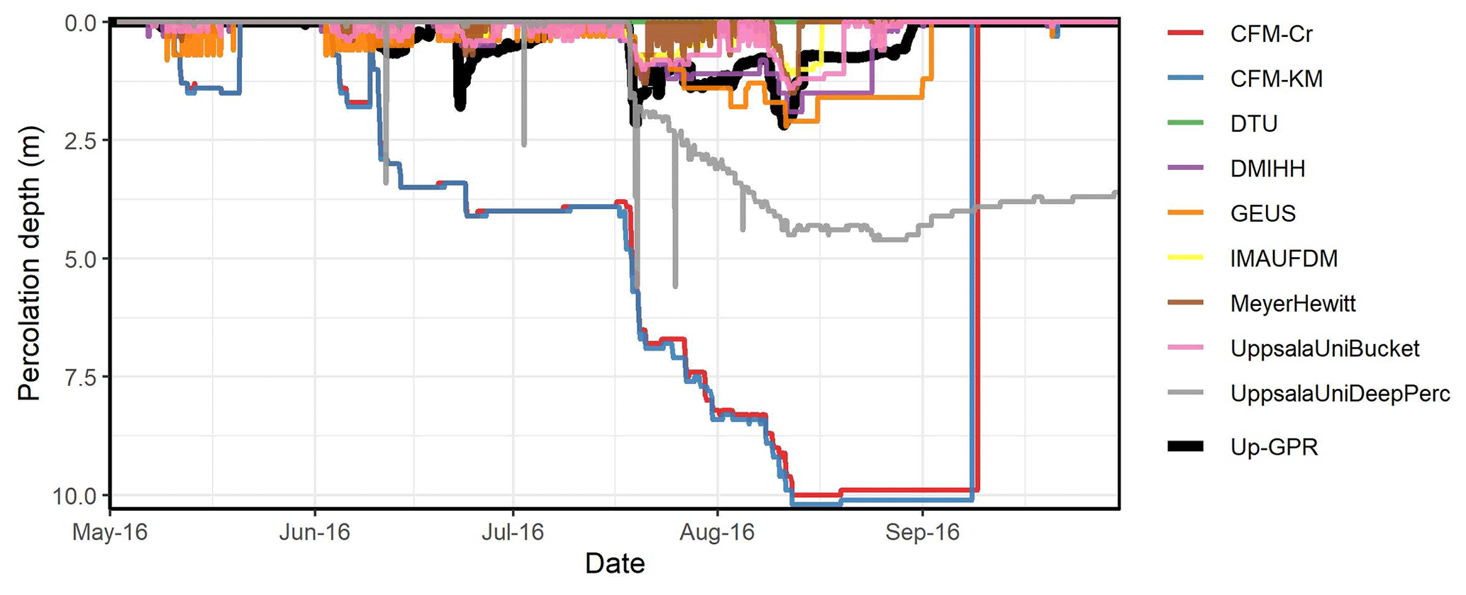
Figure 7 Comparison of the simulated (colored lines) and upGPR-derived (black line) meltwater percolation depth at Dye-2 over the 2016 melting season.

These differences in meltwater infiltration, when accumulated over a 17-year-long run, lead to large differences in firn density and temperature evolution across models (Fig. 4). Models that include deep water infiltration (CFM-Cr, CFM-KM and UppsalaUniDeepPerc) build up a thick high-density layer at 3–10 m depth. In contrast, DTU, GEUS, IMAU-FDM and UppsalaUniBucket simulate thinner, high-density layers that form each summer at the surface and are buried in the following months and years. These sharp contrasts between low- and high-density layers are smoothed in the Eulerian DMIHH and MeyerHewitt models. For each model, the simulated firn temperature at Dye-2 (Fig. 4b) and its deviation from observations (Fig. 4d) respond closely to the simulated meltwater infiltration each summer (Fig. 4c). Models that include explicitly deep percolation (CFM-Cr, CFM-Kr, UppsalaUniDeep) also present the greatest firn warming at depth due to refreezing and latent-heat release (Fig. 4b) and consequently have a positive ME ranging from 3.6 to 6.2 ^∘C (Fig. 4d). The DTU model does not percolate meltwater deep into the firn (Fig. 4c), and consequently firn temperature evolves only due to heat diffusion, which leads to a cold bias ($\text{ME}=-\mathrm{1.6}$ ^∘C, Fig. 4d). The remaining models (DMIHH, GEUS, IMAU-FDM, UppsalaUniBucket and MeyerHewitt) simulate similar interannual variability in meltwater infiltration and similar performance in firn temperature with an ME within ±1 ^∘C and R²>0.5.

The impact of these different infiltration patterns on the long-term evolution of the average firn density and how simulated firn density compares to observations are presented in Fig. 5. The standard deviation (model spread) of density reaches 161 kg m⁻³ in the top meter of firn and 141 kg m⁻³ for the 1–10 m layer (Fig. 5). Lower deviation (29 kg m⁻³) between 10 and 20 m stems from the limited time span of the simulation that does not allow the advection of the portion of firn where models disagree below 10 m depth (Figs. 4 and 5).

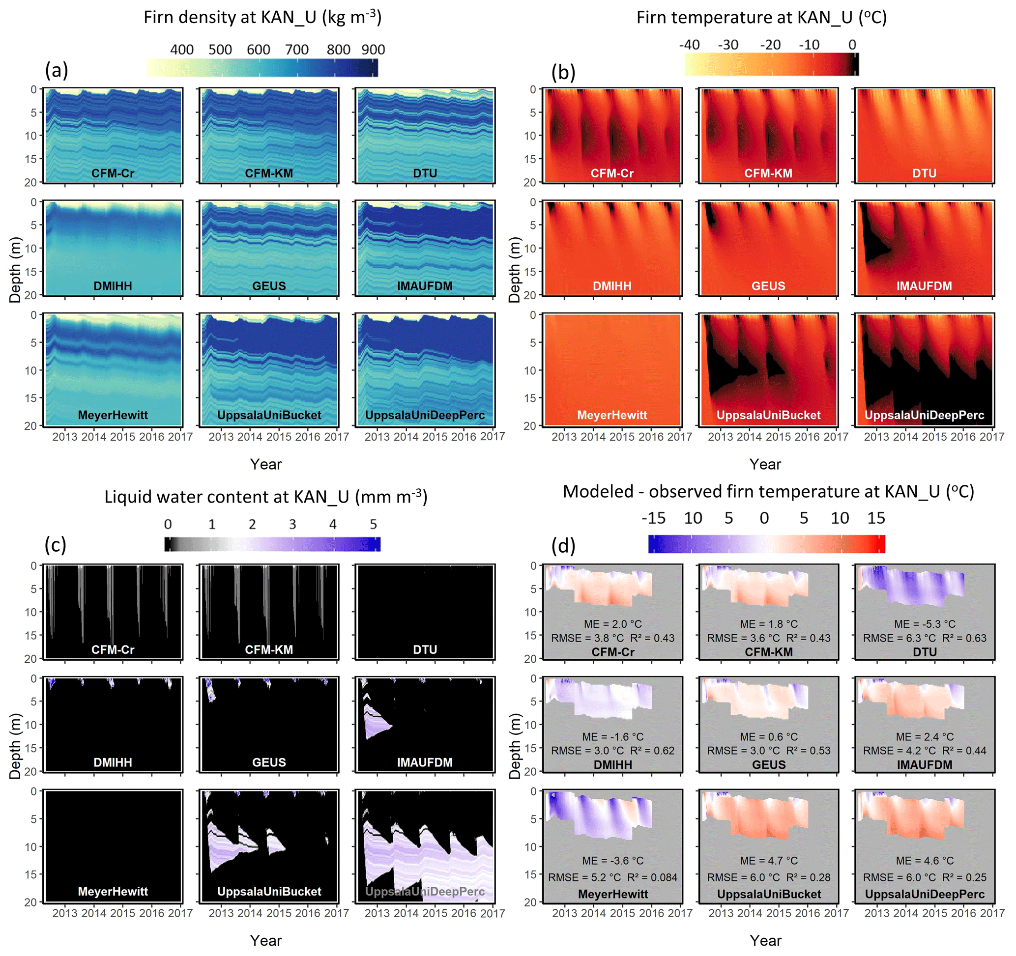
Figure 8 Simulated firn density (a), temperature (b), water content (c), and deviation between simulated and observed firn temperature (d) at KAN_U.

Figure 9 Modeled (colored lines) and observed (black diamonds with 40 kg m⁻³ uncertainty bars) average firn density for the top 1 m (a), the 1–10 m depth range (b) and the 10–20 m depth range (c) at KAN_U. Observed and simulated density profiles at KAN_U (d–g).

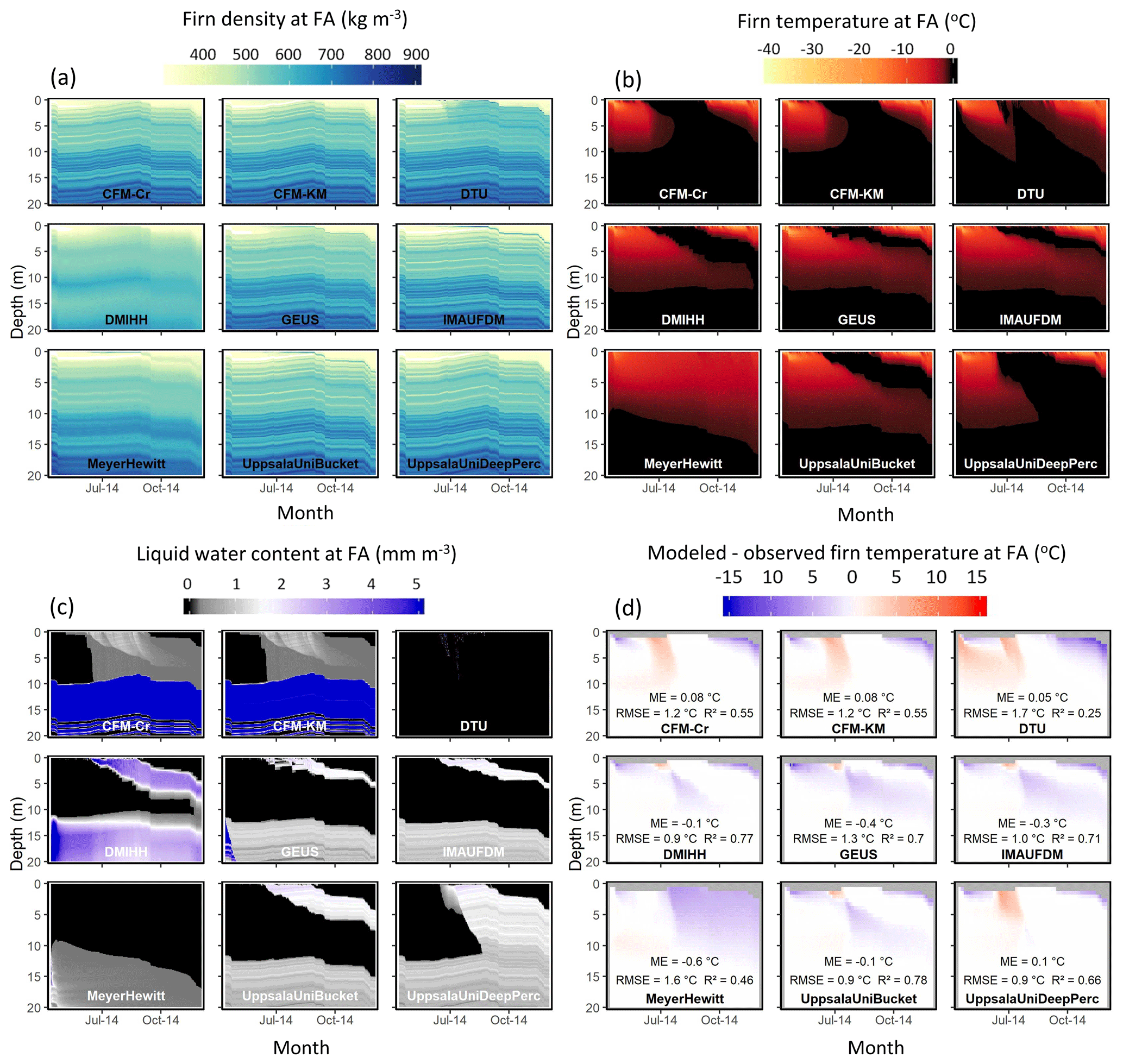
Figure 10 Simulated firn density (a), temperature (b), water content (c), and deviation between simulated and observed firn temperature (d) at FA.

The use of a more recent AWS to derive the climate forcing at Dye-2_16 allows the assessment of the firn models and their infiltration schemes in the best conditions. Over a single melt season, the meltwater infiltration and refreezing do not produce drastic changes in the simulated density profiles (Fig. 6a). Yet, the meltwater is distributed at different depths and with different timing depending on the model (Fig. 6c). The dual-domain approach of CFM-Cr and CFM-KM is visible with higher liquid water content close to the surface, corresponding to the matrix flow, and low water content infiltrating down to 10 m depth in the heterogenous percolation domain. UppsalaUniDeep, which also includes deep percolation, infiltrates water down to ∼5 m, deeper than the models using a parameterization of Darcy's law (DMIHH and GEUS models) and bucket scheme (IMAU-FDM and UppsalaUniBucket models), which do not show liquid water below ∼2 m depth (Fig. 6c). As a result of these differences in meltwater infiltration and location of the meltwater refreezing, the firn temperature differs from model to model (Fig. 6b). The deep-percolation models (CFM-Cr, CFM-KM and UppsalaUniDeep) have a marked positive bias (ME>2.6 ^∘C). The DTU model, which does not infiltrate water below the first few layers, shows a cold bias in the top 5 m of the firn, where all the other models simulate meltwater infiltration. All the other models simulate colder conditions than observed, with ME ranging from −2.5 ^∘C in UppsalaUniBucket to −1.6 ^∘C in the GEUS model.

UpGPR observations (Fig. 7) show that the meltwater did not reach below 2.5 m depth during the 2016 melt season. The melt was concentrated around three periods of increasing intensity, between May and June and a period when meltwater was continuously present in the firn, between 20 July and 25 September. Compared to the upGPR, the CFM-Cr and CFM-KM models substantially overestimate percolation depth (Fig. 7a, red and blue lines), suggesting that, in the current configuration, these models exaggerate the effects of preferential flow, at least at this location. The DTU model does not simulate any percolation, and the MeyerHewitt model simulates the presence of meltwater in short-lived, episodic pulses rather than the continuous presence of meltwater that the upGPR observed. The other models simulate a percolation depth and temporal behavior closer to the upGPR observations.

4.3 Ice slab formation: KAN_U

At KAN-U, surface melt is more intense than at Dye-2. As a result, refreezing of infiltrated meltwater forms ice slabs that can be tens of centimeters to several meters thick. This site is therefore an interesting test for the firn models to see how they handle the presence of an ice slab and the effects of ice slabs on the vertical profiles of temperature and liquid water. Note that the firn models are initialized in spring 2012 with a preexisting ice slab, which means that we do not assess the model capacity to form an ice slab; we only assess the effect of the ice slab on the evolution of the firn column.

The evolution of the density profile at KAN_U strongly depends on whether the model allows percolation past the ice slab (Fig. 8a, c). The DMIHH, MeyerHewitt and DTU models do not allow such percolation at all, and thus refreezing-related densification only occurs on top of the ice slab. The absence of latent-heat release below the ice slab causes these models to exhibit colder temperatures than observed (Fig. 8b, c). Another group of models (CFM-Cr, CFM-KM, IMAU-FDM, UppsalaUniBucket and UppsalaUniDeepPerc) does allow percolation of meltwater through the ice slab, to depths of 10–15 m. As a result, the small amount of available pore space within the ice slab is used for refreezing and is progressively filled (Fig. 8a). Nevertheless, the sealing of the ice slab in these models does not prevent the meltwater from percolating through, and meltwater refreezing continues to occur at depth and to densify the firn there. These models overestimate deep-firn temperatures compared to observations (Fig. 8d), presumably as a result of excess refreezing. In the MeyerHewitt and DMIHH models, the initial ice layers are gradually smoothed over time (Fig. 9d–g). We relate this behavior to their Eulerian framework that implies frequent averaging of firn density and temperature when mass is added or removed from the model column. Still, they keep higher density between 5 and 10 m depth, where the ice slab is. The model spread in the top 1 m average density is minimal in the spring and increases in the summer (Fig. 9a). The simulated average densities for 0–1, 1–10 and 10–20 m depth ranges compare well with punctual observations (Fig. 9a–c), but deviations between simulated and observed density profiles increase with time (Fig. 9d–g). Comparison of the simulated firn temperature to hourly observations confirms that models including deep percolation (CFM-Cr, CFM-KM and UppsalaUniDeep) and bucket schemes (IMAU-FDM and UppsalaUniBucket) infiltrate too much water at depth, resulting in a positive bias in temperature and an ME ranging from 1.8 to 4.7 ^∘C. The DTU and MeyerHewitt models do not show any meltwater infiltration or latent-heat release at depth (Fig. 8b, c). Consequently, they show lower firn temperature than observed with ME of −5.3 and −3.6 ^∘C respectively. The GEUS model uses a low but not null permeability for ice layers and thus simulates reduced infiltration through the ice slab (Fig. 8c), which leads, after this water refreezes, to firn temperatures closest to observations (ME=0.6 ^∘C).

4.4 Firn aquifers: FA

At the firn aquifer site, both melting and snowfall are high, leading to perennial storage of liquid water within the firn. In terms of firn density, vertical gradients are similar among models, but both the MeyerHewitt and DMIHH models simulate smoother profiles (Fig. 10a). This is likely due to their use of an Eulerian framework, as also seen in the results for KAN-U. Temporal evolution in density is also similar among models given the short span of the simulation. The DTU model simulates slightly denser firn in the top few meters of the column as a result of refreezing (Fig. 10a). Models which account for preferential flow (both CFM models and UppsalaUniDeep) simulate meltwater infiltration to the aquifer, although with a slight difference in timing (Fig. 10b, c). Unfortunately, the firn temperature observations do not allow us to ascertain how much water was transferred to the aquifer but only that the whole firn column was at 0 ^∘C from mid-August to late September 2014, when cold surface temperature started to diffuse into the firn. These three deep-percolation models overestimate shallow-firn temperature in summer, and underestimate shallow-firn temperature in winter when compared to observations (Fig. 10d). In the absence of ice layers within the upper firn, the DTU model simulates fast meltwater infiltration through the top 12 m and thus simulates a firn column entirely at 0 ^∘C (Fig. 10b), in accordance with firn temperature observations (Fig. 10d), but this meltwater runs off shortly after it percolates (Fig. 10c). The other models simulate a firn column that is slightly too cold, with ME between −0.1 and −0.6 ^∘C. As a result of the prescribed liquid water at depth in the initial conditions, deep-firn temperatures remain at melting point year-round in all models (Fig. 10b), with liquid water at depth in all models except DTU (Fig. 10c).

5 Discussion

The variability in simulated firn density, temperature and water content among the models and the deviation between simulations and observations (Sect. 4) can be explained by the various ways physical processes are accounted for in the models. In this section we detail what can be learned from the comparison, and we explore current knowledge gaps and potential improvements for firn models.

5.1 Dry firn and heat transfer

At Summit, comparisons with observations suggest that with appropriate forcing, the various densification formulations perform similarly and within observational uncertainty. The ability of firn models in the dry-snow area to reproduce measured density profiles has been established from previous comparisons (Steger et al., 2017; Alexander et al., 2019) and can be attributed to the fact that most densification schemes are calibrated against firn density profiles from dry-snow areas. The simulated densities at Summit show that densification schemes provide similar outputs despite modeled temperatures being slightly different (Fig. 2a, b). Still, the ability of firn densification models to simulate firn changes in a transient climate is less certain (Lundin et al., 2017) and should remain a priority for future study. We also note that densification schemes developed for dry firn are applied to wet-firn zones, and further research is needed to determine the validity of this assumption.

At Summit, the top of the initial firn density profile is advected to 10 m depth by the end of the simulation (Fig. 2). Consequently, we assess here both the models' capacity to accommodate and transform new snow at shallow depth and how models densify the initial density profile as it is advected downward. The persistence of the initial conditions consequently influences the performance of the models but has the advantage of giving all models the same starting point. An alternative strategy would have been to allow models to equilibrate with the surface forcing during a spin-up period. But such an approach would initiate models with their own spin-up result and would make it more difficult to assign differences in model outputs to either model design or different initial conditions. Our observation-based initialization was therefore deemed more suitable to intercompare the meltwater retention in different models. In spite of measurement uncertainty and firn spatial heterogeneity, the firn density and temperature measurements used to initialize and evaluate the models represent the closest estimation of actual firn characteristics. Additionally, important biases in initial firn density and temperature would lead to a visible adjustment of the simulated firn characteristics in the first months or years as the model reacts to the surface forcing. No abrupt change can be seen in the simulations (Fig. 2), which gives confidence that the initial conditions were appropriate.

Models exhibit small but clearly discernible differences in firn temperature at Summit (Fig. 2b). In our model experiments, downward advection due to accumulation was identical for all models, suggesting that this spread must be caused by the parameterization of thermal conductivity and/or the models' differing numerical schemes. Also, a suite of models exhibit colder temperatures compared with observations at Summit (DTU, DMIHH, GEUS, IMAU-FDM, UppsalaUniBucket). We interpret this as an indication that heat transfer through the firn is still not accurately handled in most firn models. The heterogeneous nature of the firn, the presence of vertical ice features in the firn, the variability in surface snow density and thermal conductivity, and firn ventilation are processes that are oversimplified or absent in the models and should be the subject of future research. Errors due to inaccurate estimates of thermal conductivity affect firn temperature, densification rates and meltwater refreezing potential. We recommend that further work investigates potential improvements of the parameterization of thermal conductivity, either using recent studies (e.g., Calonne et al., 2019; Marchenko et al., 2019) or model calibration to observed firn temperature at dry-firn locations. Other causes of mismatch between models and observations could be that certain processes (e.g., radiation penetration or variable fresh-snow density) are not provided to the models or that uncertainty in the forcing data derived from AWS observations will propagate into the model simulations.

5.2 Meltwater percolation and refreezing

Many observational studies have demonstrated that there are two pathways for meltwater to infiltrate into the firn, namely by homogeneous wetting front, also called matrix flow, and by preferential flow through vertically extended channels (e.g., Marsh and Woo, 1984; Pfeffer and Humphrey, 1996). Some of the nine participating firn models do include both percolation regimes, and others do not. The lack of preferential-flow routines has recently been described as a limitation of firn models (e.g., van As et al., 2016). Yet, little is known about how often this phenomenon occurs in the firn, how deep meltwater is transported and which process triggers preferential flow. Here, the models that explicitly include deep percolation (CFM-Cr, CFM-KM and UppsalaDeepPerc) overestimate percolation depth and firn temperature at Dye-2, KAN_U and even Summit, where the surface meltwater production is minimal. In their current configurations, the deep-percolation schemes seem less adapted for areas with minor melt. Our results suggest that until the physics of preferential flow in firn are better understood, these more complex models do not necessarily provide better results than simple bucket schemes. We recommend targeted field campaigns and laboratory studies to better understand preferential flow and using those to constrain the firn conditions and meltwater input under which deep percolation occurs. These steps are necessary to develop accurate deep-percolation schemes in firn models.

On the other hand, models that keep meltwater close to the surface because they do not include any form of deep percolation do not always show better performance. At Dye-2_16, DTU, DMIHH, GEUS, IMAU-FDM and UppsalaUniBucket all exhibit temperatures that are too cold compared with the observations. The cold bias could be due partly to an underestimation of thermal conductivity (Sect. 5.1) or to insufficient meltwater percolation. The upGPR observations at Dye-2 in 2016 indicate a reasonable percolation depth for all these models except DTU. It is conceivable that these models do simulate a reasonable percolation depth but that the volume of percolating and refreezing meltwater is underestimated. Firn temperature observations and upGPR measurements can detect the presence of liquid water, but currently, no technique allows the vertically resolved measurement of water content. The models that use Darcy's law (CFM-Cr, CFM-KM, DMIHH, GEUS, MeyerHewitt) use different formulations for the firn permeability (Table 2), which also contribute to differences in meltwater percolation and refreezing results. Firn permeability can be related to grain size and firn density (Calonne et al., 2012). However, firn grain size and permeability observations are scarce, and these variables remain totally unconstrained in current models. Future model evaluation should include the existing data where available (e.g., Albert and Shultz, 2002), and more field observations of these grain-scale characteristics should be collected.

5.3 Ice slabs

The formation of ice slabs is a complex interplay between accumulation, densification, meltwater percolation and refreezing (Machguth et al., 2016). Simulation of ice slabs by a firn model is therefore highly challenging, and success or failure to reproduce ice slabs depends on a number of processes that are closely linked and difficult to disentangle. Models that include deep percolation (CFM-Cr, CFM-KM and UppsalaUniDeepPerc) grow an ice layer of several meters thickness close to the surface at Dye-2, where no such ice slabs are observed. This model behavior can be explained by the simulation of water percolation bypassing ice layers and thus refreezing in cold underlying firn. At KAN_U, where ice slabs do exist, the DMIHH and GEUS models predict firn temperatures closest to the observations (lowest RMSE and ME) when compared to observations (Fig. 8d). The performance of DMIHH at KAN_U can be explained by the absence of meltwater infiltration below the ice slab (Fig. 8c), which agrees with recent field evidence of the ice slabs' impermeability (MacFerrin et al., 2019). In DMIHH, the blocking of percolation originates from a simple permeability criterion: a layer reaching 810 kg m⁻³ density becomes impermeable, and any incoming meltwater is sent to runoff. The choice of this value was based on work in Antarctica which found that firn permeability reaches 0 over a range of densities centered on 810 kg m⁻³ (Gregory et al., 2014). Unfortunately, such studies remain scarce in Greenland, and results do not provide a definite constraint on permeability (e.g., Albert and Shultz, 2002; Sommers et al., 2017). The DTU model uses a similar threshold density to characterize a layer's impermeability but found that 917 kg m⁻³ gave the best match with observed firn density profiles (Simonsen et al., 2013). In contrast, the IMAU-FDM model assumes that, at the horizontal resolution at which it usually operates (1–25 km²), ice layers can be assumed to be discontinuous and are therefore never impermeable. We note that the ice slab has a low but not null permeability, as illustrated by rarely observed meltwater refreezing events within the ice slab (Charalampidis et al., 2016). Unfortunately, few observations are available to evaluate the effective permeability of ice slabs at both local and regional scales and either confirm or contradict some of the assumptions made by the models. We recommend further investigation of the permeability of ice-dominated firn in relation to the firn density, the ice layer thickness, and the various spatial and temporal scales at which the firn models are used.

Two models with a bucket-type percolation scheme, IMAU-FDM and UppsalaUniBucket, use an irreducible water content formulation established by Coléou and Lesaffre (1998) from laboratory measurements. They consequently present similar and realistic percolation depths at Dye-2 (Figs. 4, 6 and 7). At KAN_U, however, in the presence of an ice slab, the two bucket scheme models overestimate percolation: this is evident from a warm bias there, relative to the firn temperature observations (Fig. 8d). We therefore conclude that bucket schemes perform relatively well in the absence of ice slabs and that they could benefit from an improved representation of flow-impeding ice layers.

Finally, we make a note on discretization strategies of firn models. In Lagrangian models, the numerical grid follows the firn as layers get buried under accumulating snow. In Eulerian models the firn is being transferred through a fixed numerical grid. The Eulerian models, DMIHH and MeyerHewitt, smooth the firn density profile, reducing and dissipating contrasts in firn density (Figs. 2, 4 and 8). This smoothing is not prevented by increased vertical resolution since MeyerHewitt has 18 times more layers than DMIHH. At KAN_U, these two models gradually lose the contrast between the layers that compose the ice slab and the firn below (Fig. 8). Therefore, Eulerian models tend to represent ice slabs in terms of a depth range with increased density rather than marked layers of ice. This limitation of Eulerian models does not prevent the DMIHH model from adequately simulating firn temperature at KAN_U (Fig. 8d) and water infiltration at Dye-2 (Fig. 6). Further testing of Eulerian models should investigate how this smoothing affects the modeled firn characteristics over longer runs and how ice slabs are represented in these models.

5.4 Firn aquifers

Like ice slabs, firn aquifers form in locations with a complex combination of accumulation, surface melt, percolation and refreezing (Forster et al., 2014; Kuipers Munneke et al., 2014). Both the thermodynamic and the hydrological components of a firn model play an important role in its capacity to simulate firn aquifers.

As a general observation, aquifers are poorly represented in the firn models considered in this intercomparison, which poses the question of the suitability of the models to simulate aquifers in Greenland. For example, horizontal water flow at depth plays a crucial role in the evolution of firn aquifers (Miller et al., 2018). However, the nine models investigated here and, to our knowledge, all firn models currently used to evaluate surface mass balance on the Greenland ice sheet are one-dimensional. As such, the water available for lateral movement in these models is sent to runoff, which is itself governed by poorly constrained parameterizations. Also, IMAU-FDM and UppsalaUniBucket do not allow for the presence of water beyond the irreducible water content: after the initialization of these models, all the excess water within the aquifer is run off instantaneously. As a result, these models are incapable of modeling actual aquifers (defined as saturated firn). Still, the regional climate model RACMO2, which includes IMAU-FDM, has been used previously to map aquifers over the entire ice sheet (Forster et al., 2014). Areas where the model showed residual subsurface water (within the irreducible water content) remaining in spring were assumed to represent areas where firn aquifers might be present. Although this approach succeeded at mapping the current firn aquifer areas, the difference between what is tracked in the model and what actually happens at a firn aquifer puts doubt on the current capacity of firn models to predict firn aquifer evolution in future climate. Other models show an intermediate type of behavior: the DMIHH model runs off excess water according to the parameterization by Zuo and Oerlemans (1996). This leads to the gradual decrease in water content within the aquifer. The GEUS model incorporates a Darcy-like parameterization of the subsurface runoff, which results in faster drainage of the aquifer than DMIHH. However, observations showed that excess water in the aquifer does not run off immediately but flows laterally and can remain in the aquifer for several decades (Miller et al., 2019).

Another challenging question for understanding and modeling firn aquifers is where and when the meltwater generated at the surface percolates down to the aquifer. Firn temperature observations show that the top 20 m of firn remained at melting point during the 2014 melt season. This indicates that meltwater from the surface reached the aquifer. The firn models do not conclusively answer how and when deep percolation to the firn aquifer takes place. Given the same surface forcing and initial firn conditions, only the models with explicit deep-percolation schemes (CFM-Cr, CFM-KM and UppsalaUniDeepPerc) infiltrate water down to the aquifer. This could indicate that the recharge of the firn aquifer has to be through heterogeneous percolation because it is the only way firn models can mimic observations. However, such a systematic infiltration through vertical channels should leave visible traces in the form of altered stratigraphy or ice columns (Marsh and Woo, 1984) or show repeatedly in firn temperature observations when meltwater infiltrates into cold firn in spring (Pfeffer and Humphrey, 1996; Charalampidis et al., 2016). Future field investigation should ascertain whether preferential flow is indeed the only process infiltrating water to the aquifer. Another interpretation could be that models using a bucket scheme (DTU, IMAU-FDM and UppsalaUniBucket) or Darcy's law (DMIHH, GEUS and MeyerHewitt) do not infiltrate water deep enough because of inappropriate irreducible water content or firn permeability for the firn aquifer site. Yet, few in situ datasets are available to constrain these firn characteristics in the models. One last possibility could be the misrepresentation of surface conditions: the melt calculated at the surface is subject to the biases and the uncertainties that apply to the so-called “bulk approach” used here in the energy budget calculation (Box and Steffen, 2001; Fausto et al., 2016). Although it was ensured that the calculated skin surface temperature agreed with observations available at KAN_U and FA, no direct observation of melt is available at our sites. Furthermore, the horizontal mobility of the meltwater, especially at high-melt sites such as FA, could lead to the injection of more meltwater at the surface than what is being melted. Therefore, more work is needed to quantify liquid water input at the top of the model in the firn aquifer region.

6 Towards ensemble-based uncertainty estimates for firn model outputs

Given the complexity of the firn models, it is difficult to propagate uncertainty and account for model assumptions and parameterizations. As a consequence, firn model outputs have commonly been given without an uncertainty range, which prevents the assessment of the robustness of model-based inferences. Taking inspiration from previous ensemble-based modeling approaches (e.g., Nowicki et al., 2016), we provide a multimodel estimation of the uncertainty that applies to any simulated value of firn temperature and density and, more importantly, to the simulated values of meltwater retention (through refreezing) and runoff.

6.1 Firn temperature and density uncertainty

We see from Figs. 2 to 7 that the spread among models increases as we move from the dry-snow area to the percolation area, peaking in areas with high-melt features such as ice slabs and firn aquifers. We suggest that the model spread presented here can provide a baseline for uncertainty whenever a single model is used. At Summit, representative of the dry-snow area, modeled average densities in the top meter of firn have a standard deviation of 13 kg m⁻³. Hence, a 2-standard-deviation (±2σ) uncertainty envelope of ±26 kg m⁻³, or ±8 %, can be used to describe the modeling uncertainty. At Dye-2, representative of the percolation area, the top 1 m average density simulated by the models has a maximum standard deviation of 145 kg m⁻³ during the 15-year-long simulation. This indicates that a substantial level of uncertainty, ±290 kg m⁻³, or ±75 %, applies to the modeled average density for the top meter. Similar uncertainty (±77 %) applies to the modeled top 1 m average density at KAN_U. As for density, the model spread in simulated firn temperature can be investigated by calculating the maximum standard deviation of firn temperature at 5 m depth among models. At Summit the ±2σ uncertainty envelope on simulated 5 m firn temperature is ±4 ^∘C. This model uncertainty envelope is wider at Dye-2, ±14 ^∘C, because of the different meltwater infiltration depths simulated by the models. At KAN_U, the uncertainty in 5 m temperature within the ice slab is ±10 ^∘C. The uncertainty range increases closer to the surface and at sites or depths where meltwater infiltration may be captured differently by the models. The level of uncertainty, both for density and temperature, increases when narrowing the depth range over which averages are calculated and conversely. This result indicates that firn models are still very variable when considering a specific depth but agree better when looking at the average firn property over a larger depth range. The uncertainty ranges provided here represent the largest deviation seen among models at any 3-hourly time step and are therefore conservative. They can nevertheless be used as a metric for uncertainty in the absence of observational constraints or when using a single model.

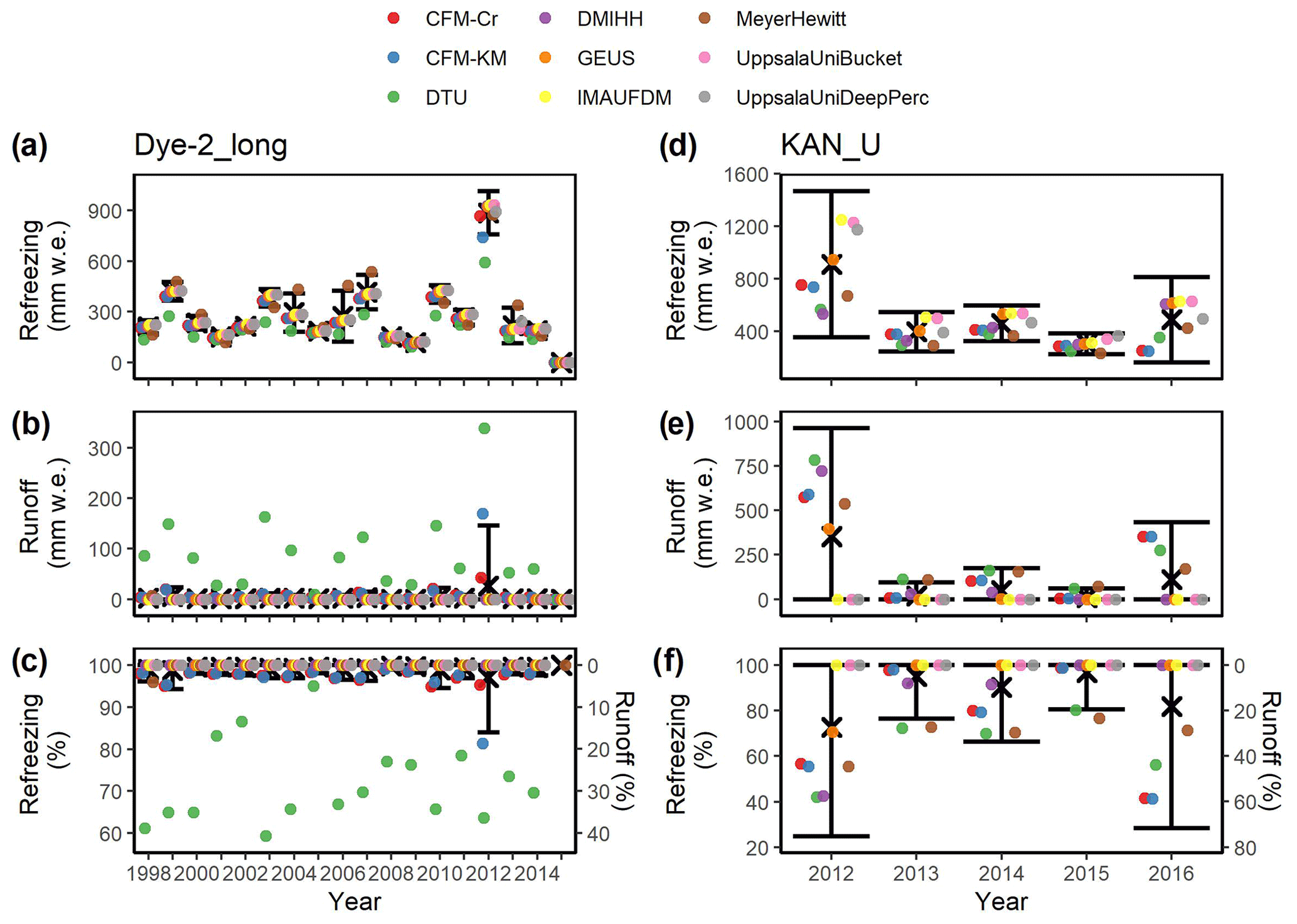
Figure 11 Simulated meltwater refreezing and runoff at Dye-2 (a, b, c) and KAN_U (d, e, f), either as yearly totals (a, b, d, e) or as fractions of yearly total meltwater input (c, f). For each panel, yearly intermodel averages (black cross) and ±2σ values (error bars) are calculated from all models except the DTU model.

6.2 Uncertainty of meltwater refreezing and runoff estimates

The differences among simulated firn density, temperature and liquid water distribution can cause them to retain and run off different amounts of meltwater and therefore affect the surface mass balance. The models agree that all meltwater is retained, meaning refrozen, at Summit and Dye-2_16. At Dye-2_long and KAN_U, the intermodel average and ±2σ values can be used as a multimodel estimation of the meltwater refreezing, runoff and the uncertainty in these estimates.

At Dye-2, the DTU model produces unrealistic runoff values (Fig. 11c) because of the impermeability of near-surface ice layers blocking downward percolation and enhancing runoff. This highlights how a model designed for the dry-snow area (Simonsen et al., 2013) can fail to capture meltwater retention in the percolation area. We therefore do not consider this model in our multimodel uncertainty estimation. All the other models agree that runoff is minimal compared to refreezing at Dye-2 (Fig. 11a–c). CFM-KM and CFM-Cr are the only models that calculate minor runoff some of the years (Fig. 11b). This is likely linked to the buildup of denser firn layers close to the surface (Fig. 4) through which water in the matrix flow domain could not percolate. Even though the preferential-flow domain could infiltrate some of the meltwater at depth (Fig. 4c), this was insufficient to accommodate all the meltwater input. As a consequence, in 2012, the year with the highest meltwater input, models on average calculate that 27±119 mm w.e. is run off, 3±13 % of the meltwater input (Fig. 11b, c). The large uncertainty envelope applying to calculated runoff highlights the disagreement of models during high-melt years (Fig. 11b). In years with absent or minor runoff, the annual refreezing totals reflect the surface melt prescribed to all models (Fig. 11a).

At KAN_U, the impact of the ice slab on the surface mass balance is critical. The different simulated meltwater infiltration patterns (Fig. 8c) lead to varying total amounts of meltwater either refrozen or run off (Fig. 11d–f). The bucket schemes (IMAU-FDM, UppsalaUniBucket) and UppsalaUniDeep percolate meltwater through the ice slab and refreeze all of the input meltwater. In all the other models, the presence of ice layers prevents or slows down meltwater infiltration as well as triggers ponding and lateral runoff, including in the CFM models, where the preferential-flow domain is unable to accommodate all the incoming water. The lowest-melt year, 2015, has the lowest model spread, with 304±80 mm w.e. of the meltwater refrozen, 97±17 % of the total meltwater input (Fig. 11d, f). The highest-melt year, 2012, also has the highest model spread in annual refreezing, with 913±557 mm w.e. of water refrozen, 73±48 % of the meltwater input (Fig. 11d, f). Subsequently, the average runoff among models in 2012 is 353±610 mm w.e., about 27±48 % of the prescribed surface meltwater (Fig. 11e, f). For comparison, Machguth et al. (2016) calculated from firn cores that 75±15 % of the surface meltwater ran off at KAN_U in 2012. Although the observations are subject to considerable uncertainty, they indicate that most of the models underestimate the runoff at KAN_U in 2012. Yet, the uncertainty envelope that applies to the simulated runoff in 2012 includes both zero runoff and the observed value (Fig. 11f).

We do not evaluate meltwater retention and runoff at FA owing to the major limitations that we highlighted in the current handling of firn aquifers in firn models. Indeed, modeled runoff, traditionally defined as excess water entering an efficient drainage system and leaving the ice sheet, does not occur at FA (Miller et al., 2018). Instead, the excess water saturates the firn and slowly moves downstream within the aquifer, which none of the models can represent. In the percolation sites represented here by Dye-2 and KAN_U, the model spread generally increases with increasing surface melt and when more of that meltwater runs off (Fig. 11). This intermodel variability largely stems from the differences in meltwater infiltration and refreezing patterns, which themselves depend on meltwater input (see Sects. 4.2, 4.3, 5.2 and 5.3). We therefore highlight the disagreement of the firn models in their simulations of the meltwater retention, refreezing and runoff in the lower accumulation area of the ice sheet. High-melt accumulation areas should therefore be the subject of further field investigations to ascertain the actual meltwater retention there and better constrain firn models.

7 Summary remarks and perspectives

Nine state-of-the-art firn models were forced with mass and energy fluxes calculated from weather station data at four sites representative of various climatic zones of the Greenland ice sheet. From the intercomparison of their simulated firn temperature, density and water content and from evaluation against various firn observations, we identified specific routines within the models that are responsible for the models' behaviors. We later quantified uncertainties that apply to the firn model outputs and their evaluation of meltwater retention. We identified key topics for future development of models and for the investigation of firn processes.

We identified the following disagreements among models and discrepancies between model outputs and observations. Runoff-enhancing ice slabs were formed in certain models at the Dye-2 site, where they are not observed. At the KAN_U site, where models were initialized with a several-meter-thick ice slab according to observations, models do not agree about whether such ice layers allow meltwater infiltration or not. Models that explicitly include deep percolation allow water infiltration through the ice slab, which is incompatible with the relatively cold firn observed at depth. At the aquifer site, only deep-percolation models infiltrate meltwater to the aquifer. Nevertheless, all models misrepresent the aquifer either because of the inability of some models to simulate saturated conditions, the different timescales at which the excess water is sent to runoff or the absence of horizontal subsurface water movement. At all sites, Eulerian models smooth the firn density profile and dissipate contrasts in firn density, even in a model with high vertical resolution. Model spread and deviation between simulated and observed firn density and temperature are largest at the sites that experience more melt. Using twice the standard deviation in model outputs as an indicator of the uncertainty envelope, we found that firn models can estimate firn density within ±60 kg m⁻³ at a dry-snow site and that this uncertainty increases to ±290 kg m⁻³ for certain depth ranges at percolation sites. The similarity between modeled and observed firn density at the nearly melt-free Summit site indicates that for the top 20 m of firn, the models' densification equations perform similarly under dry-snow conditions given identical forcing. However, variability in simulated firn temperature at Summit indicates that heat transfer through the firn is still not handled consistently in firn models. Consequently, none of the tested models compared positively with observations at all four sites.

Differences in simulated firn characteristics in the nine models led to different amounts of meltwater being retained through refreezing or being lost through runoff. Models that percolate meltwater deeper (shallower) calculate higher (lower) retention through refreezing and therefore less (more) lateral runoff. The spread among models regarding annual meltwater retention is positively correlated with surface meltwater input and is maximal, on absolute values, at KAN_U in 2012, the highest-melt year. Still, during that year, the intermodel average runoff is only 27±48 % of the total meltwater input. Therefore, further work is needed to evaluate firn models where or when an even higher fraction of the input meltwater runs off.

These mixed results show that even the newest models need further development to perform satisfactorily under the wide range of climate and firn conditions of the Greenland ice sheet. We recommend the following topics for future investigations:

• More observations of firn permeability should be conducted at both the point and regional scale. Measurements of grain size and other microstructural properties would also help to evaluate the parameterizations currently used by some of the firn models for permeability. These measurements should focus on the lower percolation area, where meltwater infiltration and runoff play an important role in the surface mass balance.

• Bucket schemes, which do not calculate firn permeability, would benefit from a density-based impermeability criterion. This criterion needs to be drawn from field evidence at the scale at which the models operate.

• Recent work on firn thermal conductivity (e.g., Calonne et al., 2019; Marchenko et al., 2019) should also be used to improve the firn models. Furthermore, the impact of vertical ice features and firn ventilation on firn temperature is currently not included in any of the firn models. Firn temperature observations are now available to assess model performance.

• Eulerian models should be used bearing in mind that they gradually smooth firn characteristics. This issue does not prevent the use of such models as long as the features that are being studied (e.g., ice slab, runoff, firn aquifer etc.) are being defined in ways that are compatible with the Eulerian framework.

• A major rethinking of firn models is necessary to better represent firn aquifers. In these regions, models need to allow saturated conditions and lateral subsurface water flow either explicitly with a multidimensional model or through an adapted parameterization. More field observations are also needed to ascertain the surface meltwater input at these sites; whether near-surface drainage occurs; and, if it does, the size of such drainage area.

• Recent efforts were made to explicitly describe heterogeneous meltwater infiltration in firn models. While they allowed better performance at the firn aquifer site, they infiltrate water too deeply and produce positive biases in firn temperature at the dry-snow site and the two percolation sites. Further work is needed to understand, under various surface and firn conditions, when heterogeneous percolation occurs, how deep it should reach and how much water it should transport. Only after these questions are understood can a reliable preferential-flow scheme be developed.

• The fresh-snow density is known to have an impact on the firn model outputs but was here set to a site-invariant value derived from observations. Fresh-snow density is known to vary considerably in space and time, although no statistically robust parameterization exists up to date for the Greenland ice sheet. Future measurement campaigns and modeling efforts could help to prescribe surface snow density and to better capture its interactions with the densification and heat transfer schemes.

Considering the number of firn characteristics that remain to be investigated and the cost of field surveys, laboratory experiments could be highly valuable if they can address the boundary effects and the scale of the process being investigated as well as provide realistic surface and firn conditions. Investigation of the points listed above will collectively improve our understanding of firn and meltwater dynamics; improve the representation of these processes in firn models; and eventually reduce the uncertainty that applies to their output when assessing the surface mass balance of the Greenland ice sheet in past, present and future times.