Possible impacts of a 1000 km long hypothetical subglacial river valley towards Petermann Glacier in northern Greenland

Greenland basal topographic data show a segmented valley extending from Petermann Fjord into the centre of Greenland; however, the locations of radar scan lines, used to create the bedrock topography data, indicate that valley segmentation is due to data interpolation. Therefore, as a thought experiment, simulations where the valley is opened are used to investigate its effects on basal water movement and distribution. The simulations indicate that the opening of this valley can result in an uninterrupted water pathway from the interior to Petermann Fjord. Along its length, the path of the valley progresses gradually down an ice surface slope, causing a lowering of ice overburden pressure that could enable water flow along its path. The fact that the valley base appears to be relatively flat and follows a path near the interior ice divide that roughly intersects the east and west basal hydrological basins is presented as evidence that its present day form may have developed in conjunction with an overlying ice sheet. Experiments where basal melting is increased solely within the deep interior near the known large area of basal melting result in an increase in the flux of water northwards along the entire valley. The results are consistent with a long subglacial river; however, considerable uncertainty remains over aspects such as whether adequate water is available at the bed, whether water escapes from the valley or is refrozen, and over what form a hydrological conduit could take along the valley base.

1 Introduction

The surface of the Greenland ice sheet holds visual clues to the topography of the bedrock, which in the interior can be below 2 to over 3 km of ice. Ekholm et al. (1998) found two, roughly 75 km long, elongated depressions in the surface of the ice that were connected by a “more than 100 km long, gently curving trench”. Ice-penetrating-radar returns from the depressions were not mirror-like, which was considered a possible indication that subglacial water was being transported in the trench northward through a basal hydrological system. With improved topographic data Bamber et al. (2013) identified a “paleofluvial mega-canyon” that extends from central Greenland all the way to Petermann Fjord (Fig. 1). The Ekholm et al. (1998) features are interior sections of this “canyon”. While the feature was referred to as paleo-fluvial, Bamber et al. (2013) also suggested that the valley could have water flowing through sections of it today. Specifically they demonstrated water was routed along independent sections of the valley but not along the whole length. In situ observations of water in the valley have not been obtained to date, nor are there current plans to acquire them. Since this “trench” (Ekholm et al., 1998), “subglacial valley” (van der Veen et al., 2007), or “canyon” (Bamber et al., 2013) takes a variety of cross-sectional forms along its length, in this article we will simply refer to it in the broadest term as a subglacial “valley”. The valley extends from 74.18^∘ N, 42.54^∘ W in the Greenland interior to 80.21^∘ N, 56.46^∘ W under Petermann Glacier. As described in Bamber et al. (2013), the valley may extend further southward, but a sparsity of radar passes makes this harder to determine.

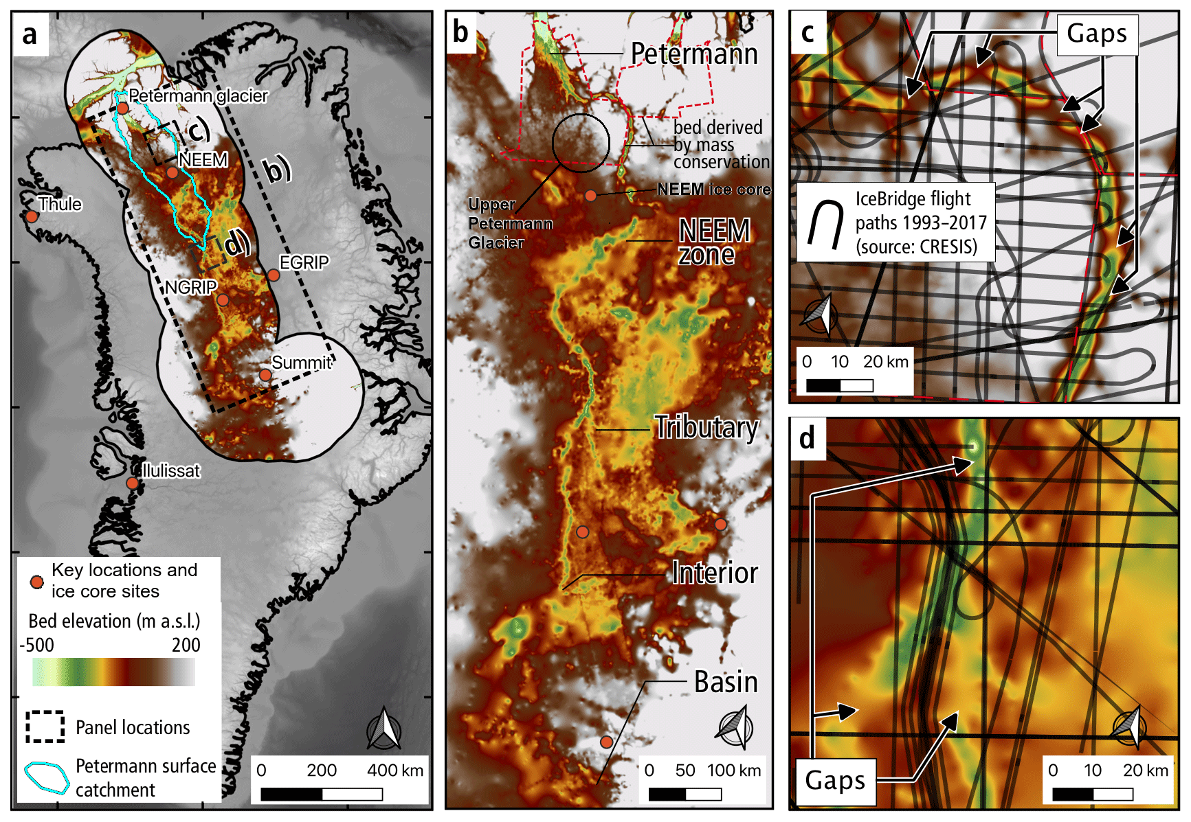
Figure 1 BedMachine v3 bed topography (Morlighem et al., 2017) between −500 and 200 m above sea level for (a) the Greenland overview with boxes for (b) the valley region and (c, d) two regions showing the IceBridge flight paths.

The term “subglacial river” has been previously used (Mooers, 1989; Clayton et al., 1999; Remy and Legresy, 2004; Popov and Masolov, 2007; Klokočník et al., 2018) to describe under ice sheet subglacial hydrological drainage within a valley, and we follow this terminology. Therefore “subglacial river” is used to cover a variety of possible non-film subglacial hydrological conduit forms such as within R channels (Röthlisberger, 1972; Shreve, 1972) or Nye channels (Nye, 1973). In addition, a subglacial river may incorporate storage within reservoirs along route that release water only over certain periods and can flow uphill in certain situations. A subglacial river beneath an ice sheet is therefore considered to have quite different properties from those of a terrestrial river.

The goal of our research is to investigate the impact of a possible continuous subglacial valley on the flow of basal water as a thought experiment, using a state-of-the-art ice sheet model. In addition, the effects on ice sheet sliding are explored as well as the impact of focussed interior basal melt on water flow along the valley. This is done in the framework of investigating whether a subglacial river along the valley base is possible.

2 Limited knowledge of bed topography

The BedMachine v3 basal topographic dataset (Morlighem et al., 2017) shows that the valley appears to be blocked by topographic rises at many points along its route (Fig. 1b, c). The mass conservation method was applied to the lowest one-sixth of the main flow line towards the Petermann Glacier, so the majority of the bed topography in this region is derived by kriging such that its error largely depends on the location of radar data. The kriging algorithm is described in Morlighem et al. (2017) as follows: “The variogram is modelled as a Gaussian function, with a sill of 100 m, a range of 8 km and a nugget effect of 50 m, to account for uncertainty in ice thickness measurements”. Based on the locations of the radar data lines that were used to generate this dataset and the limited extent of the valley bed elevation derived by mass conservation, it is clear that these rises occur only in regions where data were not obtained (two example regions are shown in Fig. 1c and d). A map of error estimates from BedMachine v3 shows the variation in error across north Greenland (Fig. 2). Errors range from 2 to ∼ 600 m with a median of 158 m along the valley. The results of Bamber et al. (2013) showed water routing along numerous independent sections of the valley; however, they inferred that water was being routed away from the valley in these data-sparse regions, and so the valley was “likely to have influenced basal water flow from the ice sheet interior to the margin”. Since these rises are due to kriging interpolation, there is currently no evidence to suggest that this valley is filled. This poses the following question: are these rises damming subglacial water flow along this conduit and negatively impacting ice sheet model simulations?

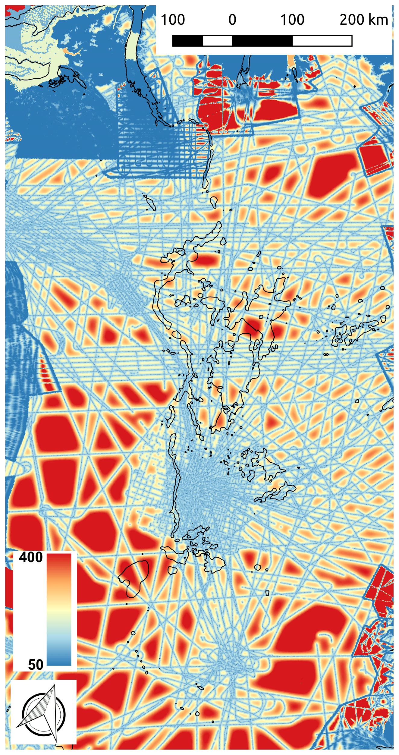
Figure 2 BedMachine basal topography error (Morlighem et al., 2017) in metres for the region from Petermann to Basin. The black contour indicates −200 m elevation.

If it is assumed that the valley is open, then the elevation of the bottom of the valley can be roughly determined by the points along its route where data were obtained. In Fig. 1b the gaps in the valley where the valley base elevation rises above −100 m occur where no data have been obtained and interpolation has smoothed out the valley. In fact, after accounting for the smoothing effects of interpolation, a roughly level incised valley will only be resolved correctly exactly at the points where the data were obtained, and everywhere else it will be shallower than it should be. Taking this into account, a rough assessment is that the valley has a base that varies between −250 and −500 m along its length from Interior to Petermann.

In order to investigate the effect of removing the rises in the valley we alter the bedrock topographic data in a way to ensure that the valley is open from Interior to Petermann (Fig. 3b). The case with the unaltered BedMachine topography downscaled to the 5 km grid is referred to as “Control” and the case with the altered open valley as “Valley”. The simulation initializations are otherwise identical so that the results only show the consequences of the modified bed topography.

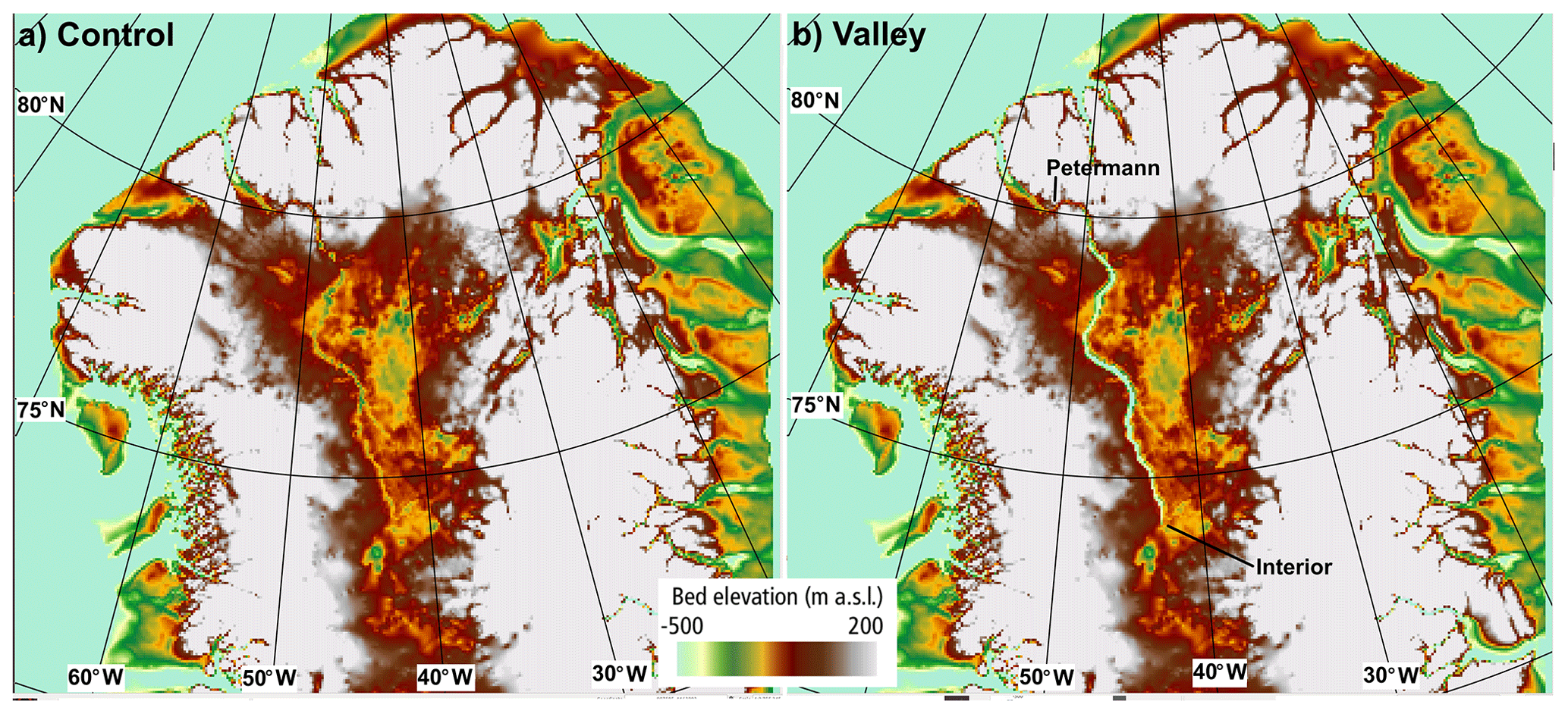
Figure 3 Basal topographic height between −500 and 200 m above sea level for (a) Control (standard SICOPOLIS input derived from BedMachine) and (b) Valley (manually adjusted from Petermann to Interior).

The topographic modification is done using a flow-oriented interpolation scheme and then taking the BedMachine and the flow-oriented scheme and extracting the lowest bedrock elevation at each grid point. Given the BedMachine topography and flight lines (Fig. 1), a polyline of the rough location of the valley is drawn using a geographic information system (GIS). A buffer of 200 km around this polyline is created, and measurements falling into this buffer are used to interpolate a new modified bed topography to be used in the Valley simulation, with the same procedure and parameters as Morlighem et al. (2017). The drawn polyline localizing outlining the valley is converted to a smooth centre line through spline interpolation. Data points situated within the valley buffer are converted from their Cartesian coordinates (x,y) towards this flow-oriented coordinate (s,n) system. This is a common reference frame, where s describes the distance of the thalweg and n is the normal in right-hand direction, and it outperforms ordinary kriging and other methods when used with an anisotropic adjustment (Merwade et al., 2006). Here the anisotropic factor was 10, with a nugget of 20 m, a sill of 30 m, and a range of 300 m. Moreover, outside of the domain of the buffer we use the same kriging parameters as BedMachine, whereas inside the buffer we use anisotropic kriging, as knowledge of the thalweg is included through a morphed coordinate system. Further details on the procedure of flow-oriented interpolation are detailed in Legleiter and Kyriakidis (2008).

For three regions, saddles are present along the valley. Bounding boxes over these saddle points are drawn that cover both the saddle and trenches within. Over these subsets a watershed algorithm called Maximally Stable Extremal Region (MSER; Donoser and Bischof, 2006) tracking is run to detect the trenches to be connected. Pixels between the trenches on either side of the saddle are found through connecting mathematical morphologic operations. These selected pixels are then adjusted by linear interpolation of the elevation information in the trenches to make a seamless passage.

The along-valley profile (Fig. 4g) indicates that our introduced valley is deeper in the interior than in the BedMachine data. The cross sections along three flight lines across the valley (Fig. 4a, b, c) indicate the valley sides have similar slope angles on the 5 km grid to the observed. Three more example cross sections (Fig. 4d, e, f) in regions of high BedMachine error (away from flight lines) show the consequent failure to resolve the valley.

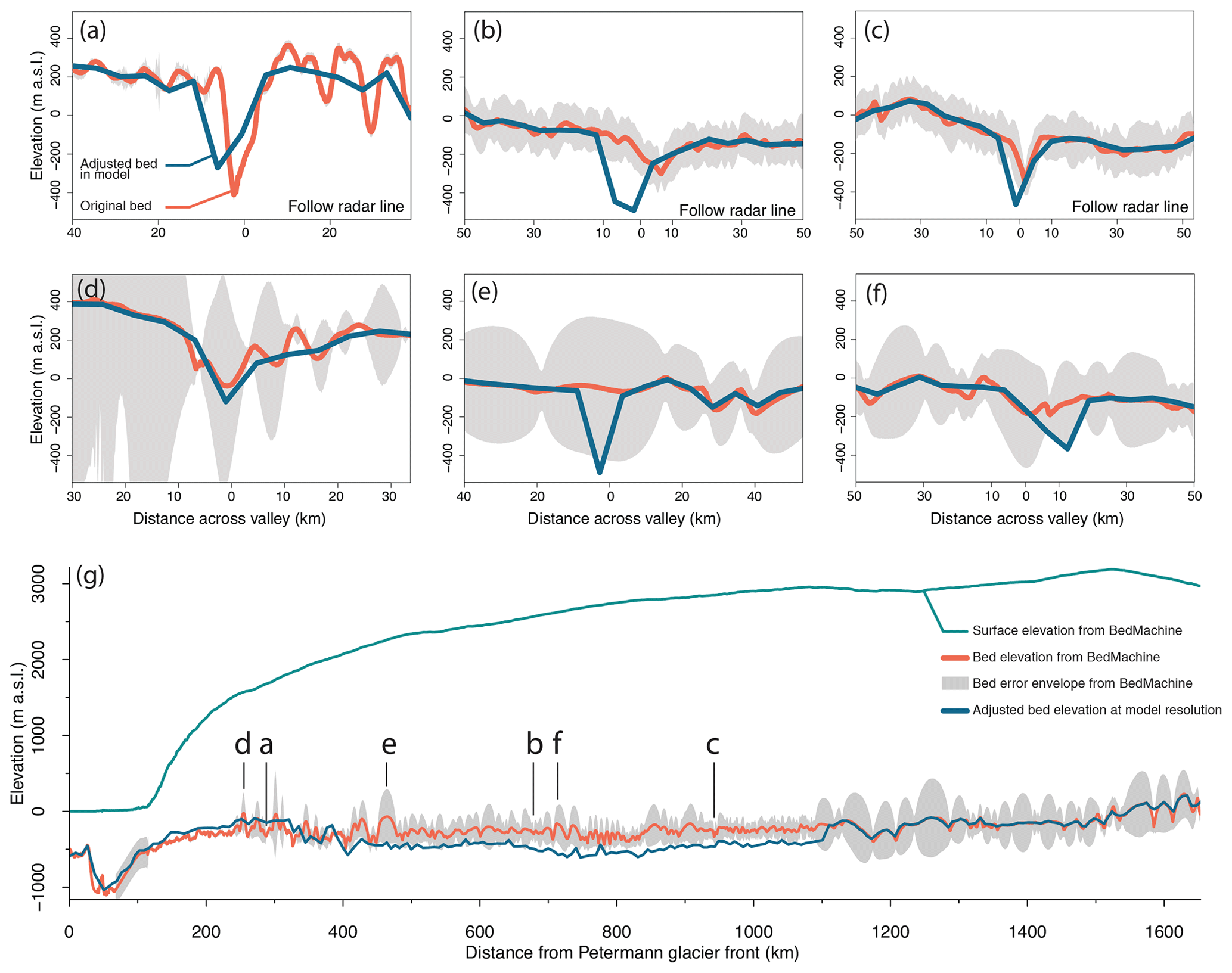
Figure 4 Across (a–f) and along (g) valley profiles from BedMachine v3 bed topography (Morlighem et al., 2017) and the adjusted bed elevation used in our model. The error envelope is derived from error estimates provided in BedMachine. Reduction in error depends on the proximity to radar data as shown in lines a–c that are parallel to flight lines or the use of mass conservation to derive bed topography which covers the region between 130 and 250 km in (g).

3 Model and methods

3.1 Spin-up until 1990

We use the SImulation COde for POLythermal Ice Sheets (SICOPOLIS, http://www.sicopolis.net/, last access: 19 October 2020) version 5.1 (Greve and the SICOPOLIS Developer Team, 2019), a polythermal ice sheet model originally created by Greve (1995, 1997) at 5 km horizontal resolution. To simulate the state of the entire Greenland ice sheet for our reference year 1990, we carry out a spin-up over the last glacial/interglacial cycle (134 kyr). The main forcing is the surface temperature anomaly derived from the δ¹⁸O record of the North Greenland Ice Core Project (NGRIP) ice core (Nielsen et al., 2018), modified by a surface temperature anomaly derived for the GISP2 site for the last 4 kyr (Kobashi et al., 2011). Except for the topographic and geothermal heat flux sensitivity tests described below, the setup is identical to the one employed for the Ice Sheet Model Intercomparison Project for CMIP6 (ISMIP6), which, in turn, is based on the one used by Greve (2019). The ISMIP6 setup is described in Goelzer et al. (2020) and shall only be summarized here.

During the last 9 kyr, the horizontal resolution is 5 km, and the computed ice topography is continuously nudged towards the (slightly smoothed) observed present-day topography. Prior to 1 kyr ago, this is done by the method described by Rückamp et al. (2019), and shallow-ice dynamics is employed. For the last 1 kyr, nudging is achieved via the “implied SMB” by Calov et al. (2018) with a relaxation time of 100 a, and hybrid shallow-ice–shelfy-stream dynamics is used (Bernales et al., 2017). Ice thermodynamics is treated by the one-layer melting-CTS enthalpy method (Greve and Blatter, 2016). The bed topography is BedMachine v3 (Morlighem et al., 2017), the geothermal heat flux is by Greve (2019), and glacial isostatic adjustment (GIA) is modelled by the local-lithosphere–relaxing-asthenosphere (LLRA) approach with a time lag of 3 kyr (Le Meur and Huybrechts, 1996). For the geothermal heat flux sensitivity tests (Sect. 3.3), only the last 9 kyr of the spin-up are recomputed.

3.2 Basal sliding and hydrology

Following the approach by Goelzer et al. (2020), we use a basal sliding law that incorporates basal hydrology. The hydrology model is coupled to the ice dynamics using a modified Weertman–Budd-type sliding law proposed by Kleiner and Humbert (2014) with the parameters determined by Calov et al. (2018). The flux and storage of water in the subglacial hydrology model are governed by both the water pressure and the “elevation potential”, which when considered together are known as the hydraulic potential (Shreve, 1972; Le Brocq et al., 2006). The basal melt rates from SICOPOLIS are used as the water input for the routing scheme, and there is no basal water source from ice sheet surface melting. Water moves in a layer only a few millimetres thick as a distributed water film where the water pressure and ice overburden pressure are in equilibrium. As such there is no explicit subglacial channelized water flow in the current formulation, and so the thin-film model is used as a guide for where subglacial water is moving and collecting under the ice sheet. Where the film is thickest along an uninterrupted path to an ocean entry is considered to be a sign of a basal environment with an increased likelihood of consisting of some form of subglacial river. The flux-routing method requires that local sinks and flat areas be removed, and this is done using a Priority-Flood algorithm which fills depressions and adds a small gradient, using the method of Barnes et al. (2014) to a basal water thickness of 10 m.

The basal sliding coefficient is determined individually for 20 different regions: the 19 basins by Zwally et al. (2012) plus a separate region for the Northeast Greenland Ice Stream (NEGIS, defined by $\ge \mathrm{50}\mathrm{m}{\mathrm{a}}^{-\mathrm{1}}$ surface velocity). This is done iteratively for the last 1 kyr of the spin-up sequence by minimizing the root-mean-square deviation between simulated and observed, logarithmic surface velocities. A detailed description of this procedure is given in Greve et al. (2020). Note that we do not recompute the optimization for the geothermal heat flux sensitivity tests (Sect. 3.3); rather, the coefficients determined by the standard bed topography (Morlighem et al., 2017) and geothermal heat flux (Greve, 2019) are used for all tests unchanged.

3.3 Sensitivity tests on geothermal flux

Two additional sensitivity tests are designed to assess whether basal water melted near the source of NEGIS is routed down the valley. The tests are referred to as ControlS, which uses the BedMachine topography as before, and ValleyS, which uses the Valley topography. Whereas the geothermal heat flux distribution of Greve (2019) is used in Control and Valley, for ControlS and ValleyS the geothermal heat flux is increased locally to generate a basal melt rate of between 0.13 and 0.14 m a⁻¹ near the source of NEGIS as shown in Fig. 5b. To do this a bell-shaped geothermal heat flux anomaly centred at 74^∘ N, 40^∘ W is introduced with a 1σ radius of 50 km and peak heat flux of 1.5 W m⁻², which creates a broader region with a comparable value to the regional heat flux of 0.97 W m⁻² estimated by Fahnestock et al. (2001). The anomaly is located over the region of enhanced basal melting at the source of NEGIS shown in Fahnestock et al. (2001, Fig. 2). The intention here is not to produce a realistic melt rate distribution but rather to test the effect of increasing melting in the interior near the source of NEGIS. However, both the maximum melt rates and the cross-sectional distribution are comparable to the cross section of derived basal melt rates of Fahnestock et al. (2001, Fig. 3).

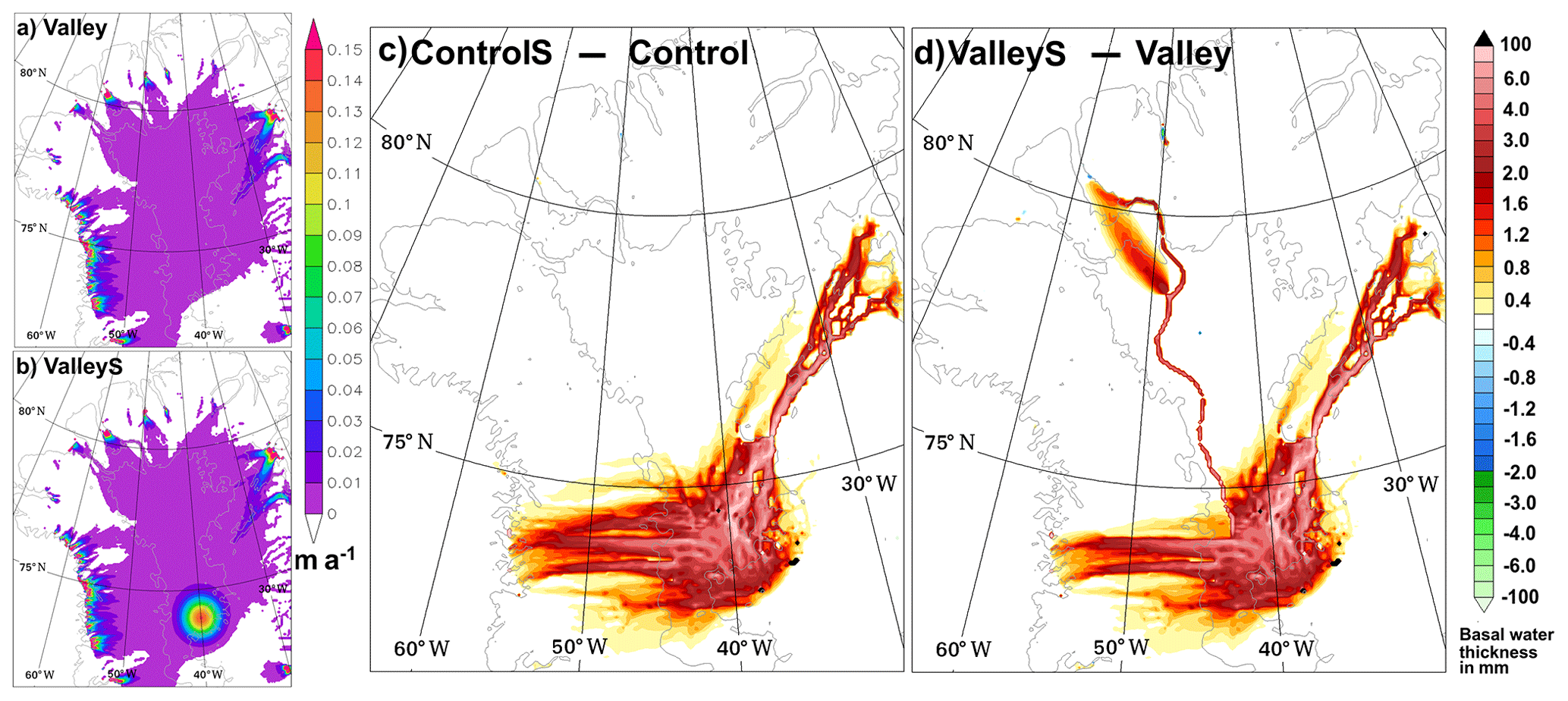
Figure 5 Basal melt rate m a⁻¹ for (a) Valley and (b) ValleyS, and basal water thickness differences (mm) for (c) ControlS – Control and (d) ValleyS – Valley.

4 Results

All results presented here are from the SICOPOLIS simulation output for the year 1990 at 5 km horizontal resolution as detailed above. To examine the effect that the introduction of an uninterrupted valley has on the simulated ice sheet, an analysis of the basal water thickness, basal water flux, and ice sheet velocity is presented.

For the Petermann catchment and northern Greenland in general, the simulated basal water thickness is affected by the introduction of the valley in several ways. In Fig. 6a it can be seen that the standard topography produces separated areas of thicker basal water along the valley but there are clear gaps between these areas. In contrast, when a continuous valley is introduced (Fig. 6b) the basal water thickness is both thicker and uninterrupted along the length of the valley all the way to Petermann Fjord. The thickest water (>10 mm) along the valley route occurs at seven locations where the Priority-Flood algorithm has been activated to a maximum thickness of 10 m. In most interior areas away from the valley there is little or no difference in the basal water thickness between Control and Valley. In particular, there is little to no effect on the basal water pathways associated with NEGIS. The interior basal water changes are relatively small because the valley follows a path close to the boundary between the east and west basal water catchments and thus has less influence on them.

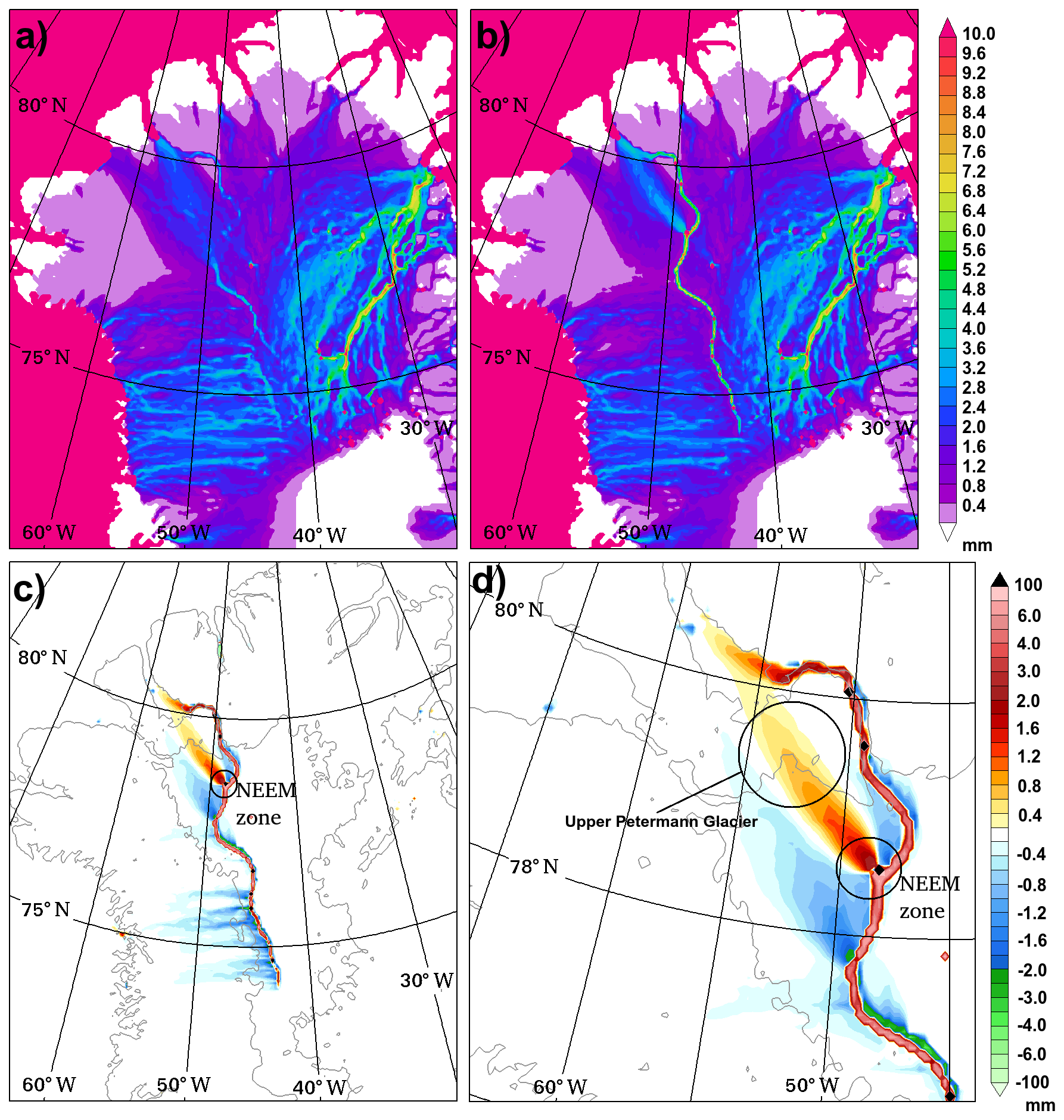
Figure 6 Basal water thickness (mm) for (a) Control and (b) Valley and basal water thickness difference (mm) (Valley – Control) for (c) northwest Greenland and (d) the Petermann catchment region.

To obtain a clearer picture of the changes to the basal water due to the introduction of the valley, the difference in basal water between the cases (Valley – Control) is shown in Fig. 6c. Doing this reveals that the increased water within the valley is surrounded predominantly by a reduction in basal water adjacent to the valley, an indication of water piracy by the valley. Basal water reduction extends to some regions away from the valley, particularly to the west of the interior section. The one region of increased basal water outside of the valley is a region that extends towards upper Petermann Glacier from the NEEM zone in Fig. 6d. The NEEM zone is defined as the area of the valley to the southeast of the NEEM ice core drilling site as indicated in Fig. 1. The effect of these changes is to redistribute the basal water under upper Petermann Glacier into a narrower and thicker plume that can also be seen in Fig. 6b.

To examine how the movement of basal water is altered by the introduction of the valley, the basal water flux is presented in Fig. 7. The valley causes a shift in basal water flux in its near vicinity, with increased flux within the valley base. Water flux streamlines give an indication that water flux is generally down the valley. In the Petermann catchment region, the increase in water flux in the valley causes a shift downstream in the subglacial water distribution where the valley crosses a region of increased flux out of the interior (NEEM zone in Fig. 7). Along this section where the valley is oriented SSW to ENE the flux just NNW of the valley is reduced in the south and then increased to the north in the region upstream of upper Petermann Glacier. This is consistent with the increase in basal water mentioned above. The simulated effect of the valley is therefore to focus maximum water flux into a narrower but more elongated region that is also shifted eastward. Four additional sensitivity tests have been used to investigate the robustness of these responses by altering the valley depth (Appendix A). These additional results indicate that the location and magnitude of this water flux out of the valley is sensitive to the valley depth due to its consequent effect on the steepness of the valley sides. Figure 7d indicates a basal water flux of 10 000 m² a⁻¹ in the valley across 5 km grid boxes upstream of the NEEM zone. This corresponds to a discharge of just 1.6 m³ s⁻¹.

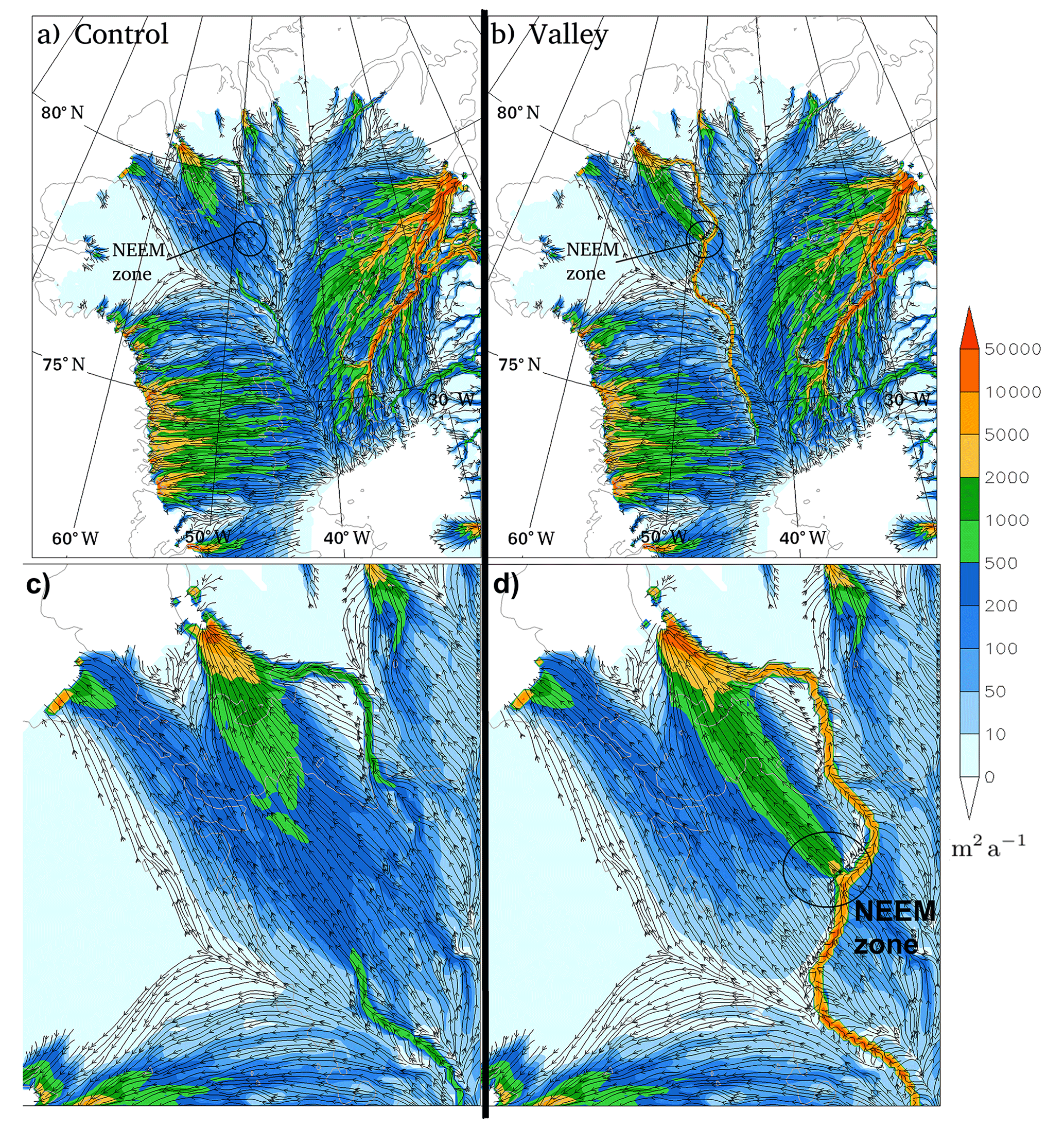
Figure 7 Basal water flux magnitude (m² a⁻¹ colours in a non-linear scale chosen to best demonstrate the distribution) and streamlines for north Greenland for (a) Control and (b) Valley. The NEEM zone marks where the greatest change occurs out of the valley as discussed in the text. In panels (c) and (d) are plots zoomed to the Petermann to NEEM zone region for Control and Valley respectively.

The rule of thumb helpful for understanding the relative roles on subglacial water flow of ice overburden pressure and basal topography is that the topographic gradient needs to be 11 times greater than, and opposing, the ice surface slope for water flowing along the bed to start accumulating (e.g. Cuffey and Paterson, 2010). Figure 8 indicates that the along-valley component of the ice surface gently slopes down-valley all the way to Petermann Fjord. This is an indication that the ice overburden pressure distribution does not oppose the flow of water towards the north and should generally reinforce it for the northern half of the introduced valley. As the ice sheet surface is very gently sloping in the interior, the basal topography and water fluxes will have a greater influence on subglacial water routing than around the edges of the ice sheet. In this situation the valley base topography could be either sloping downward towards the north or flat for water to flow northward. It appears it could be the latter.

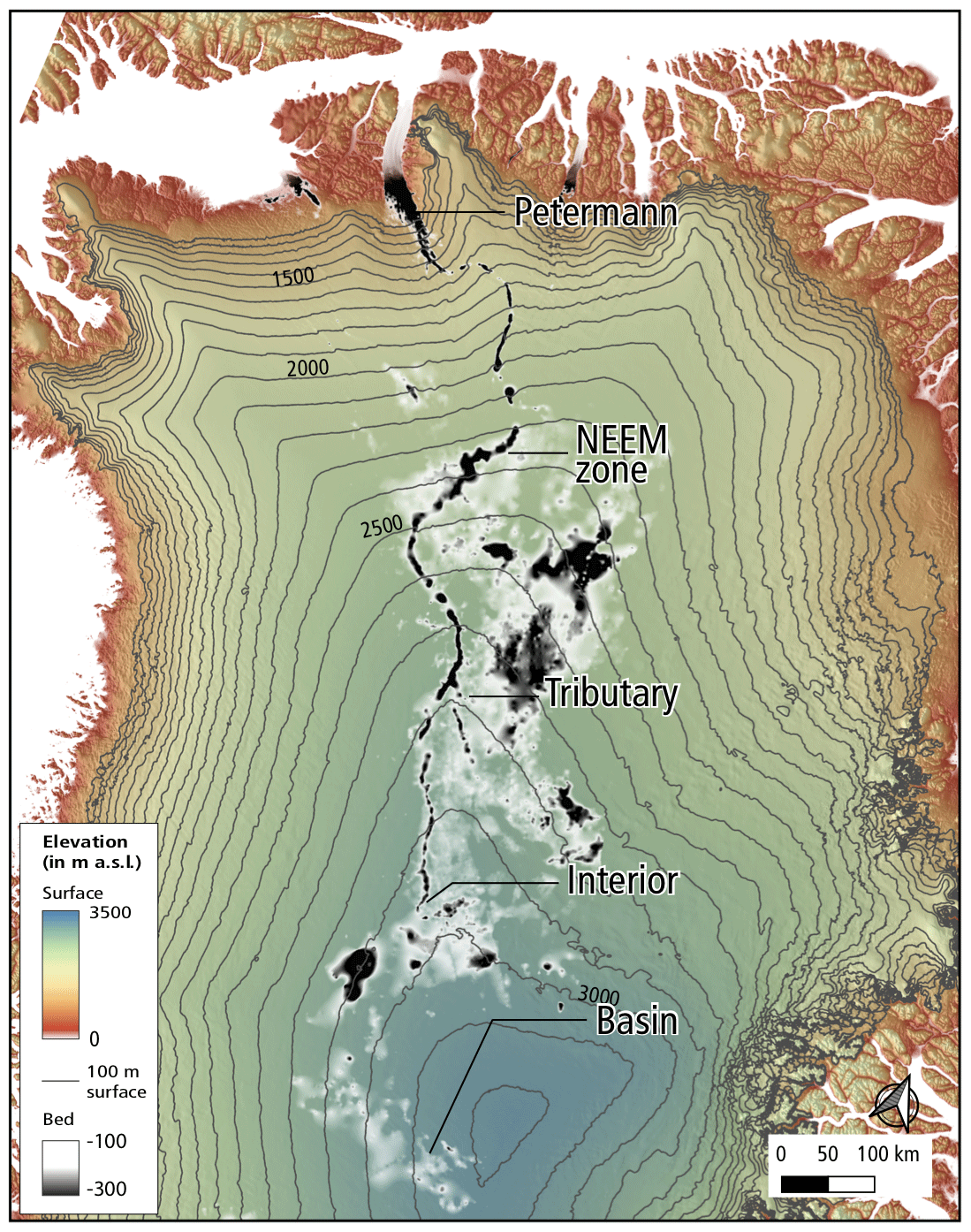
Figure 8 Surface elevation (m) with BedMachine bed elevation for −100 m or lower overlaid in grey to indicate the path of the valley.

To demonstrate the influence of the valley on simulated ice sheet sliding, Fig. 9 shows the ice surface velocity difference between Valley and Control to highlight the locations where Valley increases or decreases sliding. The sliding changes are relatively modest and localized, with only small regions at certain outlet glaciers having a greater than 10 m a⁻¹ change. Some sliding changes occur in the Petermann catchment (Fig. 9b) where sliding increases over the valley and very weakly (∼ 0.5 m a⁻¹) in the upper Petermann Glacier. These increases are consistent with the redistribution of basal water seen in Fig. 6 and could also be related to the ice thickness change due to the modification of the bedrock. The sliding changes should be viewed as demonstrations of the potential for change due to the introduction of an open valley while considering that the simulated basal hydrology is limited by its reliance on a thin-film model. Sliding changes also occur at certain outlet glaciers along the west coast as well as on the north coast around Steensby and Ryder Glacier to the east of Petermann. These changes, away from the valley and Petermann, are inconsistent across different model setups and do not show an obvious relationship to the changes in basal water distribution. They may be related to knock-on effects from the redistributions of ice mass due to the inserted valley. Considering other uncertainties and inaccuracies, the differences are too small to allow assessing which case is better compared to observed surface velocities.

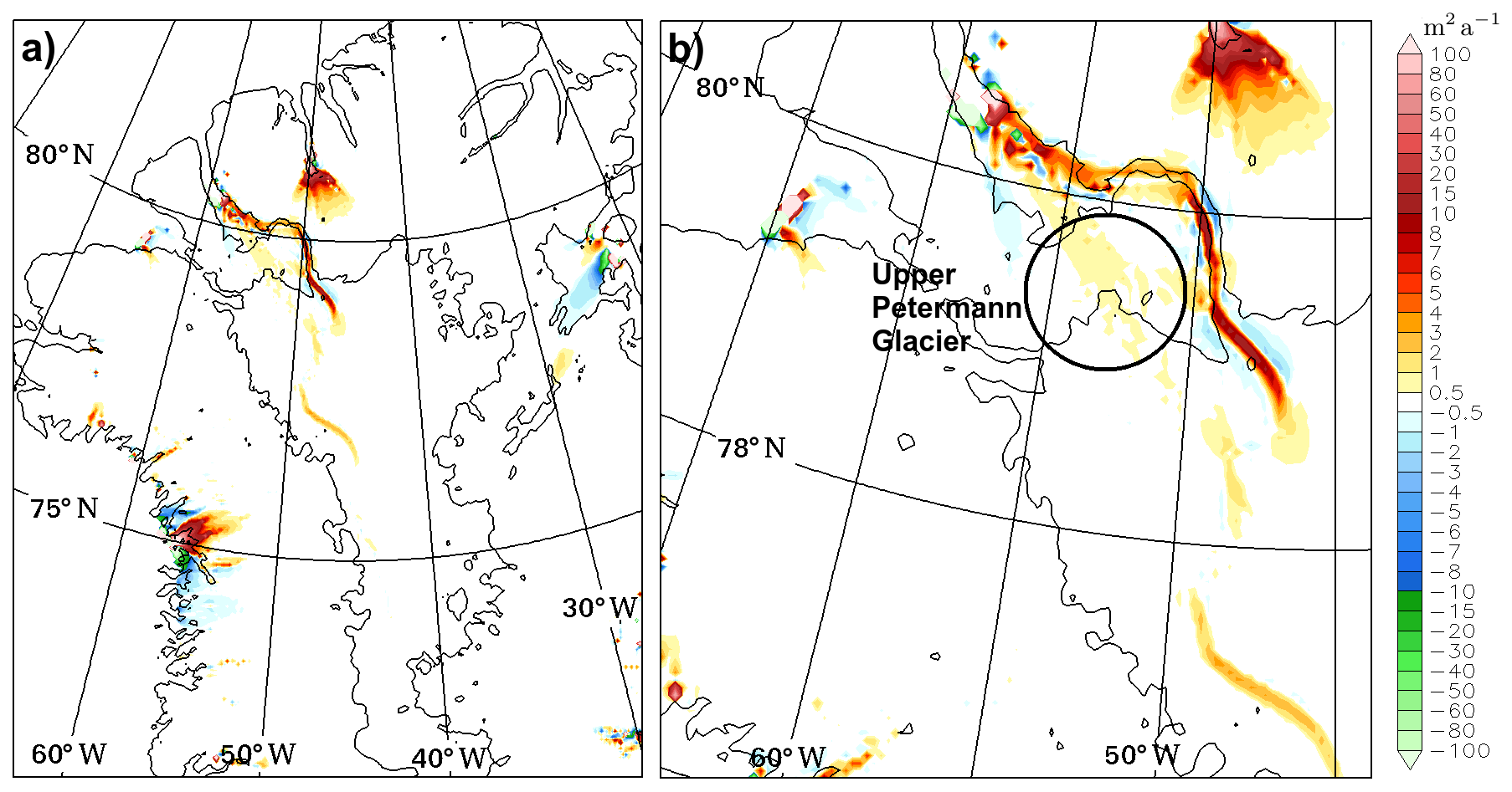
Figure 9 Surface ice velocity difference (Valley – Control) in metres per year for (a) north Greenland and (b) the Petermann catchment.

To investigate whether water is transported down the length of the valley, two additional sensitivity simulations have been completed as described in Sect. 3.3. The simulations compare scenarios with and without the open valley that also include an area of enhanced interior basal melting as shown in Fig. 5a and b. Figure 5c shows the change in basal water thickness that occurs when the enhanced basal melting region is introduced into simulations with the BedMachine topography. The greater basal melting generates larger amounts of basal water that is mostly transported down under NEGIS and adjacent regions. A lesser amount of the extra basal meltwater is transported towards the west coast. There is no change in basal water thickness along the valley route north of 76^∘ N towards Petermann Fjord, indicating that no water melted in the interior is finding its way down the valley when using the BedMachine topography. The same comparison is made in Fig. 5d; however, this time the two simulations compared have an open valley. Comparing Fig. 5c with d, the basal water distribution is similar down NEGIS, is reduced towards the west coast, and is increased along the valley down to Petermann, with the two paths, described earlier, down the upper Petermann Glacier and down the valley, evident in the northern section. This result demonstrates that simulated meltwater generated solely in the deep interior can be transported down the entire length of the valley, and it is notable that it is only at Petermann where there is any significant change to the basal water thickness across northern Greenland north of 80^∘ N. The other consequence of this is that the down-valley basal water flux upstream of the NEEM zone increases from ∼ 10 000 m² a⁻¹ in Valley to ∼ 50 000 m² a⁻¹ in ValleyS, which corresponds to an increase in thin-film discharge across 5 km grid points from ∼ 1.6 to ∼ 7.9 m³ s⁻¹.

5 Discussion

The model results indicate that the valley follows a path down a gentle ice surface slope (Fig. 8) which would imply that the ice overburden pressure lowers as the valley progresses towards Petermann Fjord. In this scenario, if a water channel were to be maintained along a relatively flat uninterrupted valley base, the overburden pressure should propel water towards the ocean outlet. This is providing that water does not escape out the sides of the valley as appears to happen to some of the water as the valley crosses the NEEM zone. If down-valley water propulsion occurs, a possibility is that it does so sporadically through the build-up, and release, of water in reservoirs along the valley route.

The results also indicate that the course of the valley in the interior runs in the vicinity of the boundary of the east and west subglacial hydrological catchments (Fig. 6a and b and shown schematically in Fig. 10). This catchment boundary occurs in this region because it is below the gentle northward ridge of highest surface ice (Fig. 8), which broadly forces the division between these hydrological basins. A consequence of this positioning is that the valley enters the Petermann surface catchment at its southernmost location (Fig. 1a). Because the gentle ice ridge is the region where water flux directed towards the east or west is at a minimum, it represents the most favourable location in the interior of northern Greenland for the development of a hydrological pathway directed towards the north. This possible relationship to the ice sheet shape could be an indication that the path of this valley has developed as a consequence of the ice overlaying it. However, while the valley appears to intersect the east and west hydrological basins in the interior it does not follow the water flux streamlines exactly, particularly as it crosses the NEEM zone. South of the Petermann surface catchment, the valley tracks roughly parallel to, and to the west of, the basal hydrological divide, while a second possible valley at “Tributary” (Fig. 1) projects towards the east of it (Fig. 10). If the bedrock were flat, there would be only one basal water route towards the north and it would be directed exactly along the hydrological divide. Perhaps a subglacial valley perfectly aligned with present-day basal water flux streamlines is not to be expected given the long period required to erode it and the different shape of the ice sheet in the past. As an example Bamber et al. (2013, Fig. 3b) indicates that the interior basal hydrological divide is shifted to the west under conditions at the last glacial maximum. Nonetheless the valley still follows a path not far off the basal hydrological divide, so it is possible that conditions favourable for subglacial down-valley water routing have existed for a long time as has already been implied by the results of Bamber et al. (2013).

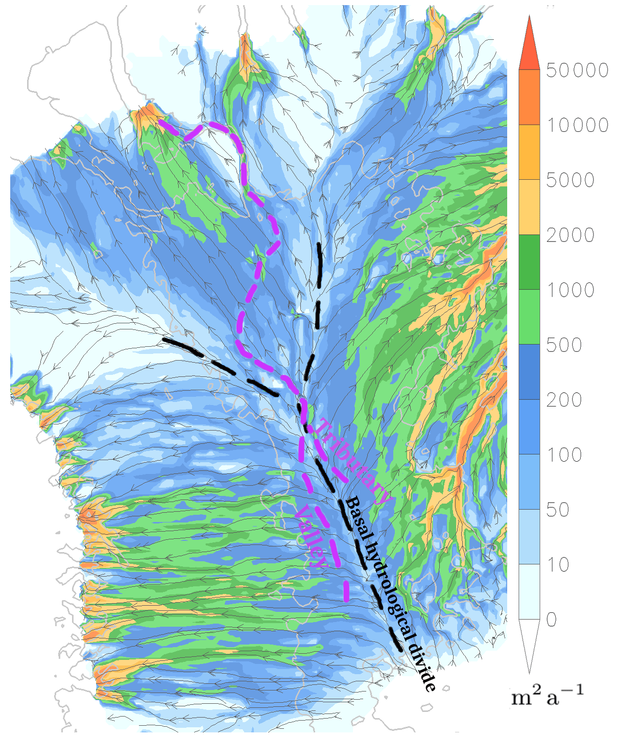
Figure 10 Schematic showing the location of the interior basal hydrological divide (black dashes) and the path of the valley and the tributary (purple dashes). The background is the basal water flux (m² a⁻¹ colours) from the sensitivity simulation that has a valley with fixed depth of −100 m (valley removal described in Appendix A).

The secondary valley, Tributary in Fig. 1, projects towards the northern section of the region of higher basal melt associated with NEGIS (Fahnestock et al., 2001) and could therefore be an additional source of basal meltwater. Also the main valley appears to continue past Interior by taking a sharp turn towards the east. This directs it to begin at the area of enhanced basal melt associated with the very source of NEGIS shown in Fahnestock et al. (2001, Figs. 2 and 3). If this is a subglacial river, then this location seems the most probable source of the majority of the discharge down the valley given the frozen or more slowly melting ice base elsewhere in the valley catchment. A distinct source at a region of high basal melt is also more consistent with subglacial water erosion rather than erosion prior to ice sheet inception when ice would not be available to melt and water sourced from precipitation would presumably be spread across the entirety of Greenland.

The valley we have inserted in the simulations has its upper end at “Interior”; however a smaller channel is evident between “Interior” and “Basin” on most, but not all, flight lines that passed over this region (Figs. 1b, 2 and 8). If these basins are connected hydrologically, it could significantly extend the catchment of the valley and imply a subglacial river over 1400 km long.

The path of such a long basal valley down an ice surface slope that appears to roughly intersect the east and west basal hydrological basins in the interior could be an indication that this feature has developed over a long period in conjunction with the ice sheet covering it. The alternative is that it eroded due to a paleo-river flowing when the ice sheet was much smaller or absent. At that time the topography would have been significantly different due to bedrock isostasy. In addition, the water flow would have been governed by gravity when conditions were ice-free. This different water flow environment would mean that it was coincidental that the same valley follows a path that is today favourable for water transport from the deep interior all the way to the coast under a thick ice sheet. Since the relationships with the ice sheet are not perfect and speculative in nature, the significance, or lack thereof, of this coincidence will need to be investigated further. However, additionally, the apparent flatness of the valley base in the interior where the ice surface is relatively flat is, just like any other river, the ultimate erosional and depositional form of a long-term active waterway. Due to bedrock isostasy it would, again, seem to be coincidental that a paleo-river system would have a relatively flat base today. One can imagine that a paleo-river valley pushed down by the weight of the ice as the ice thickened would end up today having an uneven base that depended on the evolution of the competing pressures from the ice and crustal rock. The base today is not perfectly level as it appears to vary between −250 and −500 m, but there is no obvious along-valley trend over its 1000 km length. In the absence of adequate direct observations, perhaps the topographic form of the base of this valley could, with further work, help us deduce whether this is a subglacial river or not.

Estimating the discharge down a subglacial river, which we do not know exists, in an extremely poorly observed environment is a fool's errand. However the following notes on this issue are provided as a thought experiment and to encourage future investigations. The SICOPOLIS-simulated thin-film down-valley discharge upstream of the NEEM zone is estimated as being ∼ 1.6 m³ s⁻¹ with the standard geothermal heat flux (Valley) and ∼ 7.9 m³ s⁻¹ with an included hot spot (ValleyS). Only a very rough estimate of the total discharge generated by the hot spot found by Fahnestock et al. (2001) can be made given the limited coverage of their analysis. Based on a rough outline of the detected areas of melt of 0.1 m a⁻¹, a value of order 100 m³ s⁻¹ can be obtained. The majority of this may flow northeastward under NEGIS; however, at least part of the region of consistently highest melt around the interior tip of NEGIS lies beyond the NEGIS basal hydrological catchment. A very rough estimate gives ∼ 30 m³ s⁻¹ that could be routed into the source of the valley. If the basal water that lies outside of the NEGIS basal water catchment is not being evacuated from the region, then substantial reservoirs could be continually filling until the time of release. A constant discharge of 30 m³ s⁻¹ can build up 2 592 000 m³ (2 592 000 000 L) in 1 d. Alternatively, refreezing to the ice base could reduce or eliminate this small potential discharge. Analyses such as MacGregor et al. (2016, Fig. 11) indicate that along most of the valley length, the base of the ice sheet is “likely frozen”. However, since water has been inferred to be present from ice-penetrating-radar data in a limited number of locations (Ekholm et al., 1998), and unless this water was entirely melted in place, then, based on both Bamber et al. (2013) and the results presented here, some of the detected water likely came from up the valley. As the valley approaches closer to Petermann Fjord, contributions to the discharge from summer surface melting become more likely and have the potential to overwhelm any discharge from interior basal melting. These discharge calculations are limited in many ways beyond those already mentioned; for example, there is no accounting for refreezing to the ice base or melting due to channelized water flow.

6 Conclusions

The Greenland bedrock data indicate that a subglacial valley extends from Petermann Fjord into the centre of Greenland. The valley is segmented along its route in the current bed topographic datasets used in ice sheet simulations. The rises occur where data are interpolated to fill in gaps between where radar has obtained reliable data. This suggests that the valley rises may not be real. Therefore, as a thought experiment, simulation tests have been completed to investigate the consequences of removing these rises. Opening up the valley in SICOPOLIS simulations causes water to be rerouted, leading to localized modest ice sheet sliding changes. The valley progresses gradually from thicker to thinner ice such that a lowering of ice overburden pressure could enable water along its path towards the sea. If this is the case, some of the basal water routed to Petermann Fjord may originate from melting of the deepest and oldest part of the ice sheet. Moreover, when melting is increased only in the deep interior at a known region of basal melting near the source of NEGIS, the simulated discharge is increased down the entire length of the valley only when the valley is opened. This suggests a quite finely tuned relationship between the valley form, and overlying ice can allow a very long down-valley water pathway to develop only if the valley is unblocked. The results show that even small adjustments in the bed topography to include probable features can have consequences that could affect simulations of the future ice sheet. The possibility is raised of a long subglacial river that is poorly realized in current ice sheet simulations. If this potential hydrological system has formed and/or is maintained due to the presence of the ice sheet, then it is a fundamentally different system that requires a different understanding to that of a paleo-fluvial river valley that eroded prior to ice sheet formation.

Appendix A: Sensitivity tests

The results from four additional simulations are presented here that test the sensitivity of the water routing to the valley base topographic elevation. The first three of the four tests insert 26 straight 10 km wide channels to form an uninterrupted valley from Interior to Petermann. The channels are created using the MATLAB function “inpolygon” that sets bedrock elevation grid point values within a rectangle that is aligned along the path of the valley. This method is used as it creates a flatter base than the method used in simulations Control and Valley. Consequently it is more suitable for testing the sensitivity to a particular valley base elevation. Tests are done with inserted idealized valleys at constant maximum depths of −100, −300, and −500 m and are compared to a fourth test which uses the unmodified BedMachine topography as a control simulation. The −100 m simulation effectively removes most of the segmented valley, while the −500 m case best represents the slopes of the sides of the valley. The tests use an otherwise identical method to that described in Sect. 3.1.

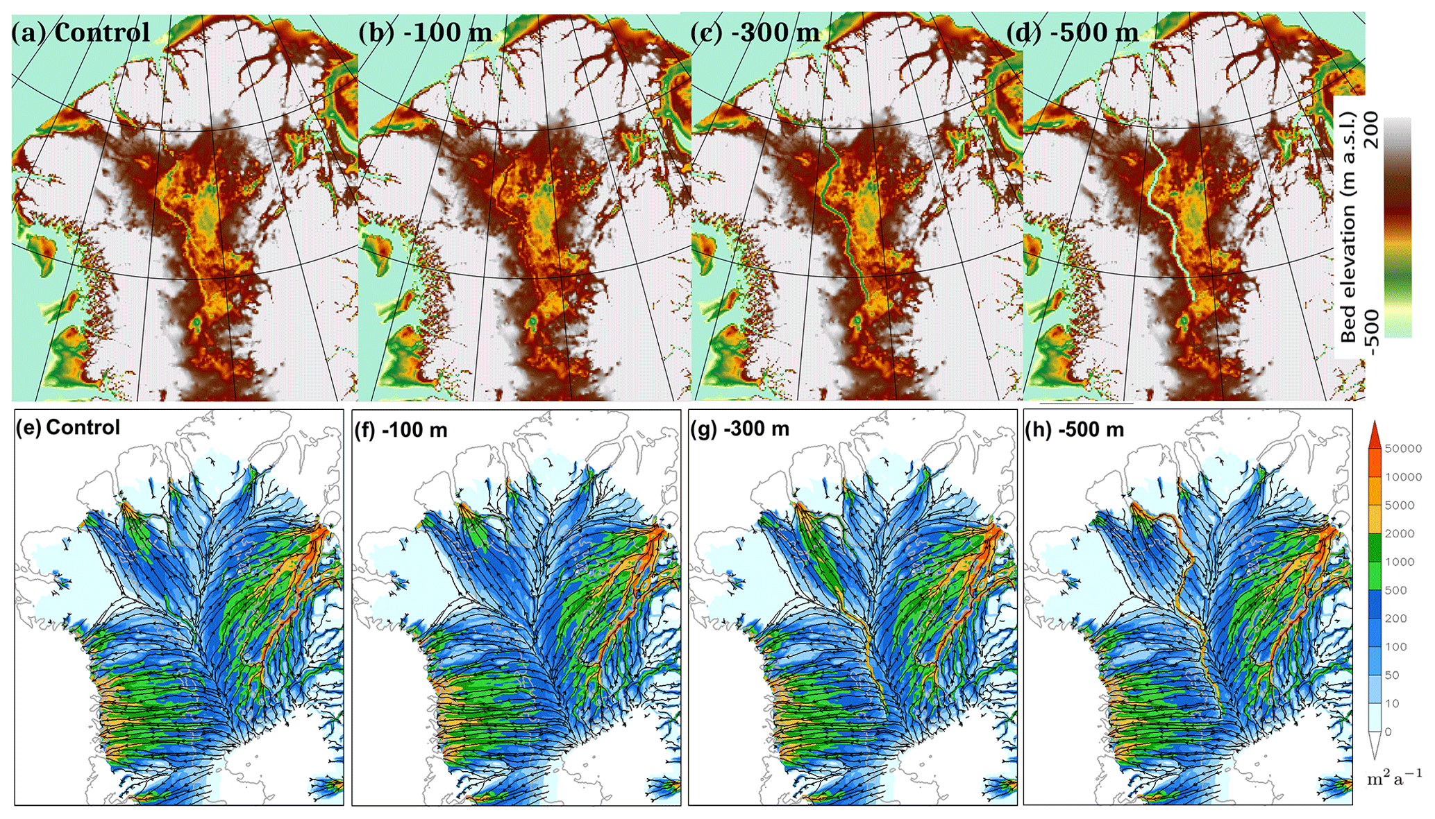
Figure A1 Sensitivity to valley depth tests. Bed topography (m) for (a) Control, and for fixed valley base elevations (relative to sea level) of (b) −100 m, (c) −300 m, and (d) −500 m. Basal water flux magnitude (m² a⁻¹ colours) and streamlines for north Greenland for (e) Control, (f) −100 m, (g) −300 m, and (h) −500 m.

The subglacial water flux for the four cases is in Fig. A1. There are large differences in water routing in and around the valley between these cases. For a −100 m valley (Fig. A1f), the northward water flux signature associated with the valley is largely eliminated. If the valley base is lowered to −300 m (Fig. A1g), increased valley water flux occurs from Interior to the NEEM zone, where water then appears to be entirely evacuated from the valley into a plume directed towards upper Petermann Glacier. For the −500 m case (Fig. A1h) the valley water flux is continuously high from Interior to Petermann, and the plume out of the valley at the NEEM zone is largely eliminated. The results confirm the finding that the NEEM zone is the region most prone to water leakage from the valley. The result for a valley base at −500 m suggest that the valley side slopes on the 5 km grid in this case are steep enough to overcome the northwestward-directed hydropotential component due to the ice surface slope. From a modelling perspective the results highlight the need to improve the bedrock topography data in the NEEM zone region.