the Creative Commons Attribution 4.0 License.
the Creative Commons Attribution 4.0 License.
 | 27 Oct 2020
The 2020 Larsen C Ice Shelf surface melt is a 40-year record high
Adrian Luckman
Harry Hendon
Guomin Wang
Along with record-breaking summer air temperatures at an Antarctic Peninsula meteorological station in February 2020, the Larsen C ice shelf experienced an exceptionally long and extensive 2019/2020 melt season. We use a 40-year time series of passive and scatterometer satellite microwave data, which are sensitive to the presence of liquid water in the snow pack, to reveal that the extent and duration of melt observed on the ice shelf in the austral summer of 2019/2020 was the greatest on record. We find that unusual perturbations to Southern Hemisphere modes of atmospheric flow, including a persistently positive Indian Ocean Dipole in the spring and a very rare Southern Hemisphere sudden stratospheric warming in September 2019, preceded the exceptionally warm Antarctic Peninsula summer. It is likely that teleconnections between the tropics and southern high latitudes were able to bring sufficient heat via the atmosphere and ocean to the Antarctic Peninsula to drive the extreme Larsen C Ice Shelf melt. The record-breaking melt of 2019/2020 brought to an end the trend of decreasing melt that had begun in 1999/2000, will reinitiate earlier thinning of the ice shelf by depletion of the firn air content, and probably affected a much greater region than Larsen C Ice Shelf.
- Article
(10673 KB) - Full-text XML
- BibTeX
- EndNote


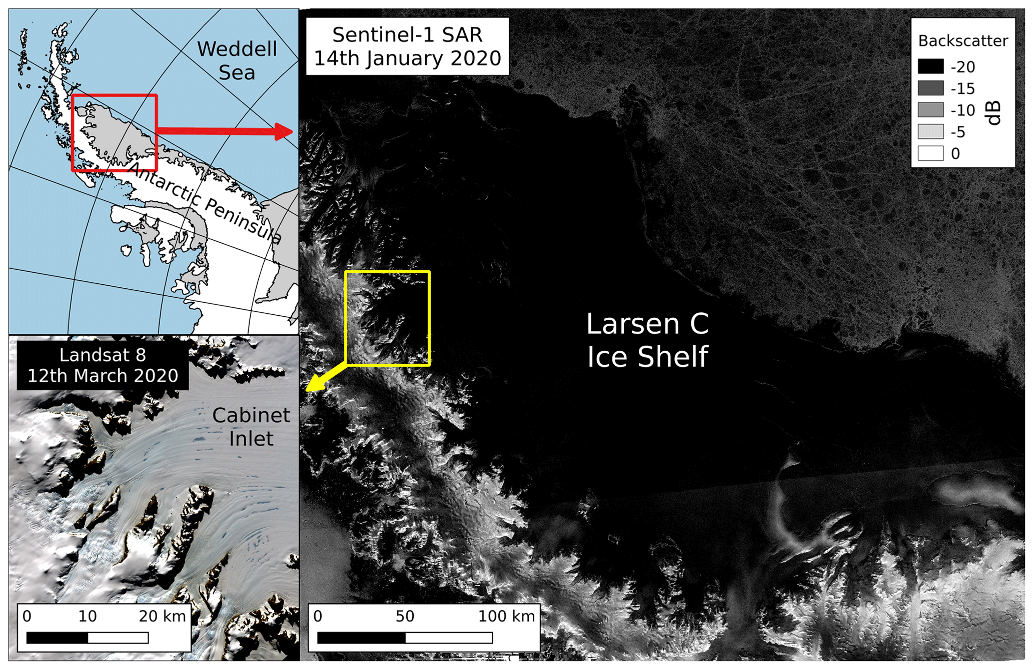
Figure 1Copernicus Sentinel-1 synthetic aperture radar (SAR) image (processed by the European Space Agency) showing widespread low backscatter on Larsen C Ice Shelf and (inset) melt ponds in Cabinet Inlet visible in a Landsat 8 image (courtesy of the U.S. Geological Survey). Coastline and grounding line were obtained from the NSIDC (Haran et al., 2014).
Surface melt and ponding on Antarctic Peninsula (AP) ice shelves has been linked to firn densification (Holland et al., 2011), surface lowering (Paolo et al., 2015), hydrofracture (Banwell et al., 2013), and eventual collapse (Scambos et al., 2000; van den Broeke, 2005). Following collapse the glaciers that feed the ice shelves have been observed to speed up (Gudmundsson, 2013), discharging more land ice to the oceans and increasing the rate of sea-level rise. Larsen C Ice Shelf (LCIS, Fig. 1) is the largest remaining ice shelf on the AP, and surface melt and ponding have led to surface lowering, concentrated in the inlets and the northern parts of the shelf, and to the formation of a large subsurface mass of ice (Hubbard et al., 2016). If LCIS were to disintegrate, in the same way as Prince Gustav and Larsen A ice shelves in 1995 (Rott et al., 1996) and Larsen B ice shelf in 2002 (Rott et al., 2002), modelling studies suggest that the dynamic response of the inland ice might be limited owing to the small amount of buttressing generated by LCIS (Furst et al., 2016). The potential sea-level contribution might only be of the order of millimetres over the next two centuries (Schannwell et al., 2018). However, removal of ice shelves has consequences other than sea-level rise with potential impacts on ocean circulation and biodiversity (Siegert et al., 2019).
Satellite scatterometer data are sensitive to the presence of water within the snowpack and can be used to monitor melt on ice shelves (Barrand et al., 2013). Although positive degree days (one indicator of conditions favouring ice-shelf surface melt) showed long-term increases from 1950 to 2010 (Barrand et al., 2013), between 2000 and 2016, a period dictated by the availability of scatterometer data, the number of melt days across the wider parts of LCIS decreased by 1 or 2 d yr−1 (Bevan et al., 2018). However, spatial and interannual variability in melt is generally high and inlets (embayments adjacent to land) prone to localized föhn-induced melting (Luckman et al., 2014) continued to experience increasing annual melt.
The negative trend in melt duration on LCIS from 2000 to 2016 was in line with trends in AP air temperatures (Turner et al., 2016) and regional atmospheric circulation patterns, and it coincided with a thickening and mass gain over most of the ice shelf (Adusumilli et al., 2018; Smith et al., 2020). In contrast to this trend, during the austral summer of 2019/2020 we observed a strong widespread fall in microwave backscatter across the shelf measured by Sentinel-1 synthetic aperture radar (SAR), indicating intense surface melt, and melt ponds could be seen in Cabinet Inlet in rare cloud-free visible imagery (Fig. 1).
It was also widely reported that air temperatures on 6 February 2020 reached a record (as yet unverified) 18.4 ∘C at Esperanza on the northern tip of the AP (https://public.wmo.int/en/media/news/new-record-antarctic-continent-reported, last access: 19 October 2020). It seemed highly likely that the record-breaking air temperatures and extensive surface melt on LCIS were both manifestations of some atypical atmospheric circulation pattern.
In this study we present calculations of the duration and temporal evolution of the melt seasons on LCIS for summer 2019/2020 and the two previous summers, thereby extending published data (Bevan et al., 2018), and compare them with the melt seasons of the past 40 years. We then discuss the wider-scale meteorology, including tropical modes of flow and teleconnections, during austral spring and summer 2019/2020 in order to investigate why this year may have been so exceptional.
2.1 Melt analyses
Previous studies of AP ice-shelf melt have utilized daily enhanced-resolution, 2.25 to 4.5 km, scatterometer data from Brigham Young University (Barrand et al., 2013; Bevan et al., 2018), where the scatterometer image reconstruction (SIR) algorithm has been used to improve the spatial resolution of irregularly and oversampled data (Early and Long, 2001; Long and Hicks, 2010). However, these reconstructed products based on Quick Scatterometer (QuikSCAT, 1999–2009) and Advanced SCATterometer (ASCAT, 2009–present) data are not immediately available and are at the time of writing available only up to the end of 2018 (e.g. https://www.scp.byu.edu/data/Ascat/SIR/Ascat_sir.html, last access: 1 March 2020). We update the SIR QuikSCAT and ASCAT melt estimates at 4.5 km resolution after Bevan et al. (2018) to include the 2017/2018 melt season. To continue the record to the present day we also produce an analysis of 2018/2019 and 2019/2020 over LCIS at a lower spatial resolution using ASCAT GDS Level 1 Sigma0 Swath Grid data from the EUMETSAT archive (http://archive.eumetsat.int/usc/, last access: 30 June 2020).
ASCAT instruments currently operate on board the MetOp-A, MetOp-B, and MetOp-C satellites. However, as we want to derive a consistent melt product for the austral years of 2017/2018, 2018/2019, and 2019/2020 and MetOp-C was not launched until 7 November 2018, we exclude data from this satellite from the study. The normalized backscatter data have an approximate spatial resolution of 15–30 km and are delivered on a 12.5 km grid.
The presence of water within the snowpack causes a sharp drop in microwave backscatter compared with cold dry snow. We record the presence of melt water at a pixel location when the backscatter is more than 2.7 dB below the previous winter (June, July, August) mean. This threshold was used in previous studies using SIR ASCAT data (C band, 5.255 GHz) (Ashcraft and Long, 2006; Bevan et al., 2018) and was based on empirical comparisons with QuikSCAT-derived melt (Ashcraft and Long, 2006). We have no reason to suspect that Level 1 ASCAT data would require a different threshold, and melt patterns and variability have anyway been found to be insensitive to changing the threshold between 2 and 4 dB (Wismann, 2000). MetOp-A and MetOp-B observations over LCIS are acquired between 02:00 and 06:00, as well as between 06:00 and 10:00 local time, and we combine all mid-beam observations within a 24 h period by taking the minimum backscatter value from all observations to maximize the chance of detecting melt.
Melt days are then summed over the austral year August to July. We emphasize here that this method detects the presence of liquid water rather than the process of melting and that subsequent references to melt in the text should also be interpreted to mean the presence of liquid water.
We use the detection of melt to calculate three measures. First, we calculate annual maps of melt duration by accumulating the total number of days of melt per year for each pixel. These datasets are then resampled to a 2 km grid and masked to the ice-shelf area which includes Larsen D but excludes the Larsen C area that calved in July 2017. Second, we calculate the total area of ice-shelf melt per day, and third we calculate melt indices to enable a quantitative interannual comparison of melt over the whole ice shelf. The melt index is the product of the number of melt days per pixel times the pixel area, summed over the area of LCIS.
There are two periods of Level 1 ASCAT data missing in the newly analysed period: 22 d from 12 December 2017 to 2 January 2018 and 30 d from 17 December 2018 to 15 January 2019. We assess how much the data gaps might lead to underestimates of melt by calculating the melt indices for these short periods using the SIR ASCAT data for the equivalent periods in 2017/2018.
We extend the analysis back from 1999 to 1979 using passive microwave data from the Scanning Multichannel Microwave Radiometer (SMMR, 1979–1987) and the Special Sensor Microwave/Imager (SSM/I, 1989–2017), selecting the descending orbit 18.0 and 19.35 GHz horizontally polarized channels, respectively (Picard and Fily, 2006). In a similar way to the scatterometer method, we use a brightness temperature (Tb) threshold relative to the winter mean, which corresponds to the Tb-M method described in Ashcraft and Long (2006). Melt is detected when the daily Tb is more than 30 K above the previous winter mean (Picard and Fily, 2006). Time of day of overpass has been shown to have an impact on melt detection, but the effect is not significant on the Antarctic Peninsula where melt is common and persistent. Choosing the descending passes for SMMR and SSM/I minimizes the impact of instrument change (Picard and Fily, 2006), even if the overpass times are not at peak melt, and matches the ASCAT times more closely. Bevan et al. (2018) discussed the impact of acquisition time of day with respect to differences between SIR QuikSCAT and ASCAT melt detection on LCIS. The 2008/2009 year of overlap showed that the melt index based on the QuikSCAT morning data was 3.3×10⁶ melt days km2, and the melt index based on ASCAT was 3.4×10⁶ melt days km2.
2.2 Atmospheric circulation
The evolution of the atmospheric circulation during austral spring–summer 2019–2020 and a comparison to historical variability are described using the ERA5 reanalyses (Copernicus Climate Change Service (C3S) (2017): ERA5: Fifth generation of ECMWF atmospheric reanalyses of the global climate; https://cds.climate.copernicus.eu/cdsapp#!/home, last access: 2 April 2020). These data are available on ∼ 30 km grid and cover the period January 1979–March 2020. We also look at present sea ice concentrations and sea surface temperatures (SSTs). The sea ice concentrations were downloaded from the National Snow and Ice Data Center (NSIDC, Cavalieri et al., 1996) and are available as monthly means on a 25 km grid for January 1981–March 2020. The SSTs are the NOAA Optimal Interpolation SST v2 data (Reynolds et al., 2002). These data are available as weekly means on a 1∘ grid and are available from January 1982 to March 2020.
We monitor the latitudinal position of the high-latitude westerly jet using the Southern Annular Mode index (Marshall, 2003). The SAM index is the difference in zonal mean surface pressure at 40 and 65∘ S. A positive value of the index indicates a strengthened and poleward-shifted westerly jet, while a negative value indicates a weakened and equatorward-shifted jet. Historically, high positive SAM is associated with warming on the east (leeward) side of the Antarctic Peninsula (Marshall et al., 2006) due to föhn winds and local southward advection of warmer air from the north.
The El Niño–Southern Oscillation (ENSO), or its atmospheric component the Southern Oscillation Index (SOI), is often considered an indicator of how tropical weather patterns are affecting the high southern latitudes and Antarctic melt (Tedesco and Monaghan, 2009; Trusel et al., 2012; Barrand et al., 2013). ENSO has generally been found to be inversely correlated with Antarctic surface temperature and with melt, but regionally, and particularly on the AP, the impact can depend on the combined phases of ENSO and SAM (Nicolas and Bromwich, 2014; Clem et al., 2016).

Figure 2Number of melt days in (a) 2017/2018 based on SIR ASCAT data, (b) 2017/2018 based on Level 1 ASCAT data, (c) 2018/2019 based on Level 1 ASCAT data, and (d) 2019/2020 based on Level 1 ASCAT data. The background image is Copernicus Sentinel-1 2019 mean backscatter.
Alternatively, the Indian Ocean Dipole (IOD) is the Indian Ocean equivalent of an El Niño, and its phase (Dipole Model Index, DMI) is calculated as the difference in SST anomalies between two regions of the Indian Ocean (Wang et al., 2019). We also therefore investigate DMI to indicate how tropical weather patterns were having an effect on higher latitudes.
Comparing the maps of melt on LCIS (Fig. 2) we can see that the 2017/2018 melt based on Level 1 ASCAT data (Fig. 2b) compares well with the SIR data (Fig. 2a). Based on Level 1 data melt in 2018/2019 is very low in contrast to melt in 2019/2020, which appears to be particularly intense with up to 139 melt days in the south-west inlets. Melt distribution follows the typical pattern of enhanced melt in the inlets close to the mountains superimposed on a general south-to-north gradient of increasing melt (Bevan et al., 2018, Figs. 6, and A1). Inspection of daily images of backscatter (not presented) shows that patches of melt, mostly focussed on the inlets close to the mountains, begin in October 2019, but from January 2020 through February and into March the entire ice shelf has very low backscatter, indicating the persistent presence of liquid water.
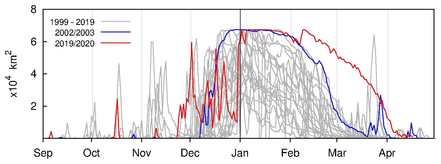
Figure 3Ice-shelf melt area. The 1999–2019 curves are based on the three sets of scatterometer data: SIR QuikSCAT, SIR ASCAT, and Level 1 ASCAT.
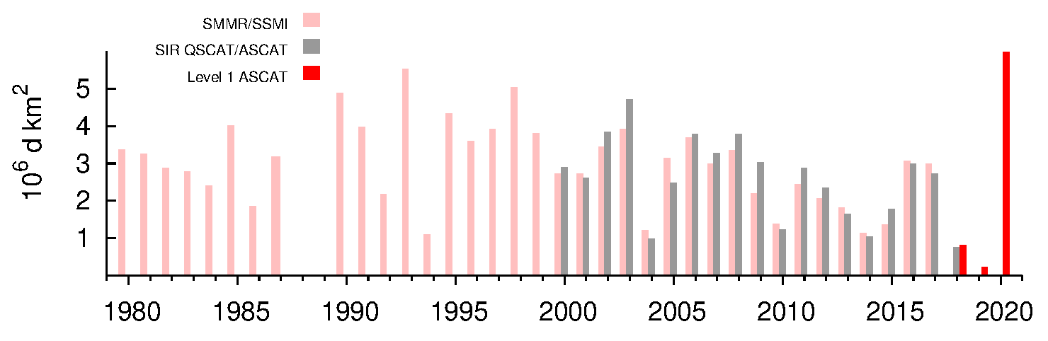
Figure 4Melt index time series based on brightness temperatures from SMMR and SSMI, SIR QuikSCAT and ASCAT data, and Level 1 ASCAT data.
The temporal evolution of melt area shows intermittent melt episodes during the last 4 months of 2019, not dissimilar to previous years, followed by a steep increase from early January 2020 that persisted until the end of March (Fig. 3). This persistence of large areas of melt is very unusual in comparison with the previous 20 years with the exception of 2002/2003 (highlighted in blue in Fig. 3).
The time series of melt indices (Fig. 4) shows good agreement between the passive radiometer (SMMR and SSM/I) and scatterometer methods of detecting melt. The series confirms the exceptional nature of 2019/2020 – the melt index in 2019/2020 at 6.0×10⁶ melt days km2 is the highest in the record. Based on the SIR ASCAT data for 2017/2018 the melt indices for the short 22 and 30 d periods when Level 1 ASCAT data in 2017/2018 and 2018/2019 are missing are only 0.17 and 0.34×10⁶ melt days km2, respectively; i.e. the majority of melt happens later in summer. The 22-day figure suggests that the melt index for 2017/2018 based on Level 1 ASCAT data of 0.80×10⁶ melt days km2 is not greatly underestimated because of the missing data, and the good agreement between SIR and Level 1 melt indices shown in Fig. 4 can be trusted. The 30 d figure, whilst for the previous year, suggests that the low melt index for 2018/2019 of 0.22×10⁶ melt days km2 may be as high as 0.56×10⁶ melt days km2, which would still be the lowest on record.
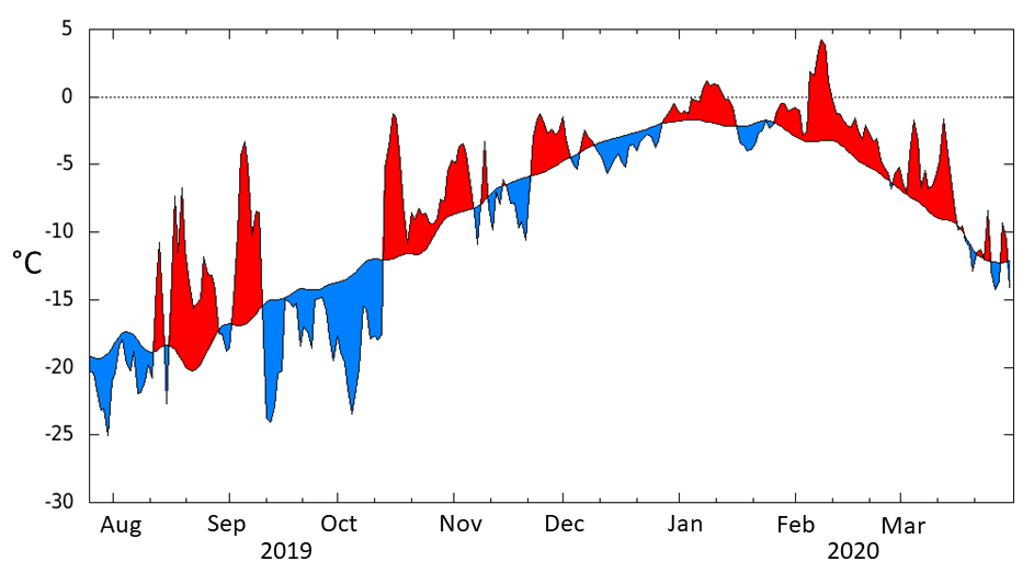
Figure 5Mean daily and 1979–2019 mean ERA5 2 m air temperatures averaged over the area −65 to −70∘ N, 60 to 65∘ W. Positive (negative) anomalies are shaded red (blue).
The ERA5 2 m air temperatures (Fig. 5) show repeated intervals of anomalously warm air over the ice shelf but that it was not until late December or early January 2020 that air temperatures were consistently above −2 ∘C and anomalously warm. Melt is able to occur and persist above −2 ∘C as surface energy budget calculations on LCIS have shown that surface temperatures can exceed 2 m temperatures by up to 2 ∘C under calm cloudy conditions (Kuipers Munneke et al., 2012). In addition Fig. 5 shows the mean daily temperature, and it is very likely that temperatures were higher for a large part of the day.
Turning to the indices of atmospheric flow, while there was only a weak positive El Niño (https://origin.cpc.ncep.noaa.gov/products/analysis_monitoring/ensostuff/ONI_v5.php, last access: 1 May 2020) toward the end of 2019 and into 2020, a very strong positive IOD began in winter and was matured during austral spring (August–November 2019), peaking at over 3 standard deviations above the mean in October 2019, making it one of the strongest IODs on record (Fig. 6). Monthly SAM indices for October to December 2019 were strongly negative at −1.97, −4.42, and −1.78, but in January, February, and March they increased to 0.57, −0.36, and 2.05.
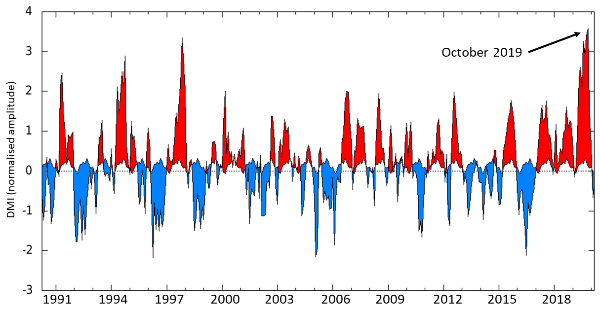
Figure 6Standardized time series of the Dipole Mode Index difference between the SST averaged in the western equatorial Indian Ocean (50–70∘ E and 10∘ S–10∘ N) and the south-eastern equatorial Indian Ocean (90–110∘ E and 10∘ S–0∘ N) based on Extended Reconstructed Sea Surface Temperature data (ERSST, https://www.ncdc.noaa.gov/data-access/marineocean-data/extended-reconstructed-sea-surface-temperature-ersst-v5, last access: 2 April 2020).
The Level 1 ASCAT data have allowed a rapid but robust assessment of the two most recent LCIS melt seasons, with the SIR/Level 1 overlap period of 2017/2018 allowing a validation of the duration and location of melt derived from Level 1 data. The analysis shows that melt durations in 2018/2019 and 2019/2020 were at the extreme ends of that observed on LCIS since 1979. In 2018/2019, melt appears to continue the general trend of decreasing melt that began in the early 2000s, and the melt index was the lowest on record. In 2019/2020 intense and widespread melt covered the ice shelf, in a manner not observed since 2002/2003 (Bevan et al., 2018).
The large-scale atmospheric flow leading up to and through the extreme melt season in 2019/2020 consists of a sequence of unusual events. A very strong IOD developed in winter and persisted through early summer 2019 (Fig. 6). Historically, a positive IOD during austral spring acts to excite a stationary Rossby wave train into the Southern Hemisphere extratropics, which places an anticyclone to the south-west of Cape Horn (Fig. A2d). The associated southerly surface winds near and to the east of the AP produce colder-than-normal air temperatures (Fig. A3d) and an increase in sea ice concentration in the Weddell Sea (Fig. A4d). Similarly, to the west of the Peninsula, the positive IOD typically acts to drive northerly surface winds that act to warm the surface and decrease sea ice in the Bellingshausen Sea. The observed anomalies of circulation in the lower troposphere and the air temperatures and sea ice concentration during August–September 2019 (Figs. A2a, A3a, and A4a) match well with what typically occurs during a positive IOD event.
Then, in early September 2019, a sudden stratospheric warming (SSW) occurred, which was historically early and of comparable magnitude to the only previous major Southern Hemisphere sudden stratospheric warming that occurred in late September 2002 (Lim et al., 2020, SPARC, 2019: SPARC Newsletter No. 54, January 2020, 48 pp., available at https://www.sparc-climate.org/publications/newsletter, last access: 19 October 2020) when, intriguingly, the summer melt on LCIS was also exceptionally high (Figs. 3 and 4). SSWs weaken or even completely reverse the westerly stratospheric polar jets and generate extreme weather events throughout the polar and subpolar regions of the Southern Hemisphere in the following months as the weakened or reversed vortex descends to the surface, resulting in low SAM. The coupling of the 2019 SSW to the surface triggered persistent record negative SAM from the third week of October through the end of December.
As a result of the SSW and development of negative SAM, we might have anticipated a further increase in sea ice and strengthening of the cold conditions on and east of the AP during November and December that had been generated earlier by the positive IOD. However, the swing to negative SAM altered the mean flow through which the IOD-forced stationary Rossby wave train was propagating. The easterly anomalies in the high latitudes acted to more strongly refract the IOD-forced Rossby wave train back to the tropics (Fig. A2b). The net effect is that from late October through to the end of December, while the IOD event was, unusually, persisting and the SAM was strongly negative, a cyclone replaced the anticyclone to the west of the AP (Fig. A2b). The resulting north-westerly and north-easterly flow on either side of the AP acted to warm the surface, remove the enhanced sea ice in the Weddell sea (Fig. A4b), and drive southward Ekman transport of warm SSTs towards the AP (Fig. A5b and c).
In contrast, it is unlikely that the weak warm El Niño of the 2019/2020 summer was a trigger for the melt event because the Pacific–South American (PSA) wave-train signature of stationary Rossby waves excited by a warm El Niño (Karoly, 1989) would normally manifest as anomalously high pressure over the Amundsen Sea to the west of the AP (Mo and Higgins, 1998). This anomaly is not apparent in Fig. A2b and c, and the wave-path latitude in Fig. A2a–c is shifted south by about 10∘ in the Pacific sector compared with that associated with a PSA wave train.
The preceding events were undoubtedly unusual and by delivering broad-scale ocean heat to the region by the end of December were likely to have acted as important precursors to the anomalously high presence of melt during January and February. Although the influence of the IOD and SSW on the circulation disappeared by the end of December, during late summer an anticyclone was established over the AP (positive 500 hPa geopotential height anomaly, Fig. A2c), resulting in poleward surface flow that tapped into the ocean heat, keeping air temperatures high on the AP (Fig. 5). Two factors will have contributed to the continued detection of surface melt into March 2020. Firstly, during summer, short wave radiation is able to penetrate the snow pack, particularly when the surface is at or near melting (Kuipers Munneke et al., 2012), causing subsurface melt. Secondly, microwaves are also able to penetrate the snow pack so that reductions in backscatter due to absorption are sensitive to subsurface as well as surface liquid water. In other words, the persistence of subsurface melt water following extreme and prolonged surface melt will have contributed to the scatterometer-derived melt area (Bevan et al., 2018). This effect is what reduces the impact of the less-than-optimal overpass times for the passive microwave and ASCAT observations of melt on LCIS.
This record ice-shelf-wide melt following a period of low SAM indices and weakened westerlies at first seems to contradict observations that strong westerlies enhance melt on eastern AP ice shelves via föhn warming. However, we note that in extreme melt years such as 2019/2020 the melt extends across the full width of the shelf but that the deep föhn events required to produce melt this far from the mountains (Elvidge et al., 2015) are relatively rare (Cape et al., 2015). In addition, the temperature anomalies produced by föhn events are much smaller during the summer than other seasons (Kuipers Munneke et al., 2018; Wiesenekker et al., 2018) and account for a smaller proportion of melt. The fact that the 2019/2020 melt is linked to regional warm advection rather than local föhn warming means that it is likely to have affected a wider region than just LCIS.
Increasingly strong SAM (Arblaster and Meehl, 2006) and more extreme positive IODs (Cai et al., 2014) predicted under high-greenhouse-gas-emission scenarios may act in opposition with regard to AP warming as they decrease or increase sea ice over the Weddell Sea, respectively. As we have revealed in this study the implications for eastern AP ice-shelf melt are further complicated by Southern Hemisphere SSWs, and it is not yet understood how global warming will affect the occurrence or intensity of SSWs in either hemisphere; indeed there is not yet a consensus on the best way to define an SSW (Butler et al., 2015).
The 2019/2020 LCIS melt season was longer and more intense than any observed over the last 40 years, bringing to an abrupt halt the apparent 21st century decline in surface melt. The extreme melt through the summer of 2020 is likely to have reinitiated thinning of the entire ice shelf through loss of firn air content. Although late winter and early spring 2019 were cold on and around the AP as expected under a strong positive IOD, this was interrupted by an SSW which caused the ongoing IOD to bring warmth to the region in December and into January when normally the low SAM indices would have meant cold conditions. The majority of the 2019/2020 melt was detected in January to March 2020, probably as a result of anticyclonic conditions over the shelf drawing on abnormally warm and ice-free surrounding oceans. Even once the actual process of melt had ceased, the liquid water was likely able to persist within subsurface layers and hence be detected by scatterometer.
These atypical atmospheric phenomena are indications of how tropical and extratropical weather patterns can impact high latitudes. Further investigation into these teleconnections and the implications for future ice-shelf stability is an important area for continued research. Surface energy budget modelling on LCIS would also be able to shed light on the exact balance of fluxes contributing to the melt.
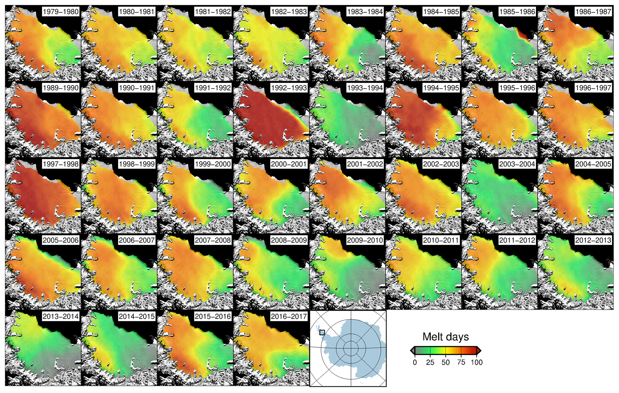
Figure A1Time sequence of annual melt duration based on passive microwave data (SMMR, 1979–1987; and SSM/I, 1989–2017). Summers 1987/1988 and 1988/1989 are missing due to data unavailability.

Figure A2(a–c) Anomalies in ERA5 500 hPa geopotential height relative to the 1982–2019 climatological mean based on daily data for (a) 1 August to 15 October 2019, (b) 17 October to 31 December 2019, and (c) 1 January to 15 March 2020. The averaging periods were shifted slightly to maximize the signal of the Indian Ocean Dipole (IOD) during August through mid-October and then the abrupt appearance of negative Southern Annular Mode (SAM) as a result of the coupling of the polar stratospheric warming down to the surface that occurred beginning around 17 October 2019 and lasting through the end of December 2019. Both the IOD and the negative SAM disappeared during January to mid-March 2020. Shading indicates where the magnitudes of the anomalies are larger than 1.6 standard deviations, thus indicating where the positive anomalies fall above the 95th percentile and the negative anomalies below the 5th percentile. (d–f) Linear regression of the 500 hPa geopotential height anomaly onto the Dipole Mode Index (DMI) for the equivalent period based on monthly data from 1982 to 2019. Shading indicates regression is significant at p<0.10. The regression coefficients are scaled by 1 standard deviation of the DMI so that the maps represent the height anomaly that would be accounted for by 1 standard deviation in DMI for (d) August to October, (e) November to December, and (f) January to February. The blue arrows depict idealized Rossby wave-train ray paths and highlight the shortening of the Rossby wavelength in November/December 2019. The regressions were computed using the Royal Netherlands Meteorological Institute (KNMI) Climate Explorer (see http://climexp.knmi.nl/, last access: 2 April 2020, Oldenborgh and Burgers, 2005)
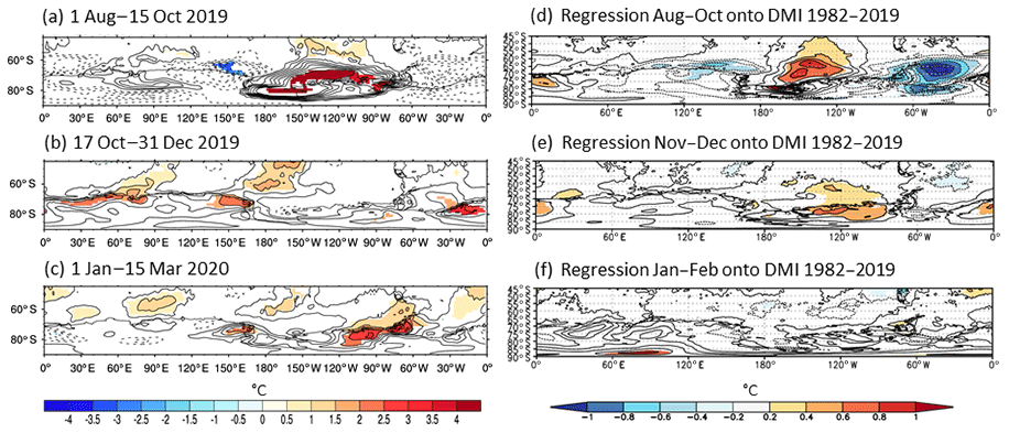
Figure A3As for Fig. A2 but for ERA5 2 m air temperatures.
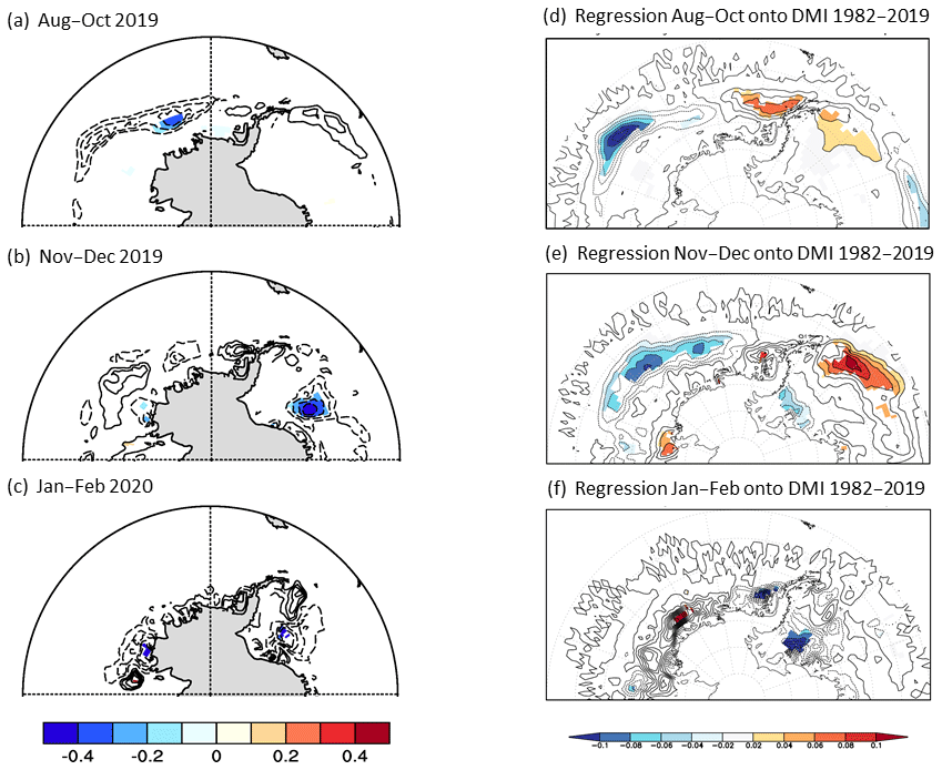
Figure A4(a–c) Anomalies in sea ice concentration relative to the 1982–2019 climatological mean for (a) August, September, and October 2019; (b) November and December 2019; and (c) January and February 2020. Shading is as in Fig. A2. (d–f) Linear regression of sea ice concentration anomaly onto the Dipole Mode Index (DMI) for the equivalent period based on data from 1982 to 2019. Shading indicates regression is significant at p<0.10. The regression coefficients are scaled by 1 standard deviation of the DMI so that the maps represent the anomaly that would be accounted for by 1 standard deviation in DMI for (d) August to October, (e) November to December, and (f) January to February. The regressions were computed using the Royal Netherlands Meteorological Institute (KNMI) Climate Explorer (see http://climexp.knmi.nl/, last access: 2 April 2020, Oldenborgh and Burgers, 2005).
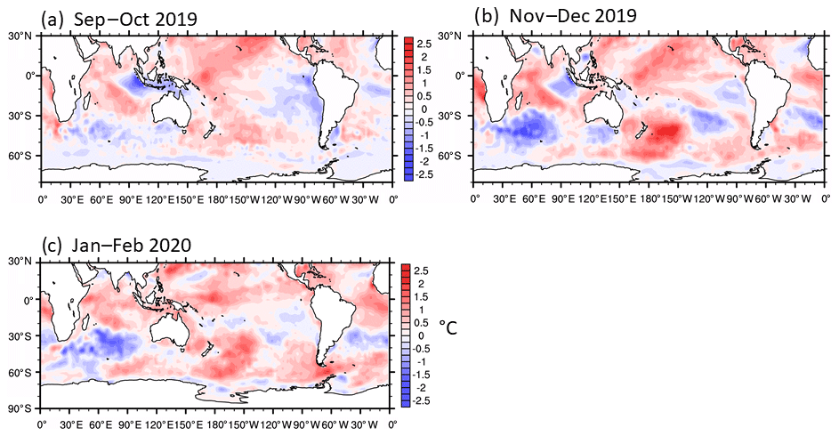
Figure A5Sea surface temperature (SST) anomalies relative to 1982–2019 mean for (a) September and October 2019, (b) November and December 2019, and (c) January and February 2020. SST data are NOAA OI v2.
The NERC Polar Data Centre hosts GeoTIFFs of melt duration based on the SIR QuikSCAT/ASCAT and Level 1 ASCAT data (https://doi.org/10.5285/e3616d28-759e-4cca-8fae-fe398f9552ba, Bevan and Luckman, 2018; and https://doi.org/10.5285/cfa4cc5d-3ea9-4c3c-8d6b-6b92a81bb2af, Bevan and Luckman, 2020).
The authors declare that they have no conflict of interest.
The Nimbus-7 SMMR Pathfinder Daily EASE-Grid Brightness Temperatures, version 1 (Knowles et al., 2000), and DMSP SSM/I-SSMIS Pathfinder Daily EASE-Grid Brightness Temperatures, version 2 (Armstrong et al., 1994), were downloaded from the NSIDC. NSIDC also supplied the sea ice concentration data (Cavalieri et al., 1996). The ERA5 data were made available by the Copernicus Atmosphere Monitoring Service information (2020); neither the European Commission nor ECMWF is responsible for any use that may be made of the Copernicus information or data it contains. SAM index data were obtained from the British Antarctic Survey (http://www.nerc-bas.ac.uk/icd/gjma/sam.html, last access: 19 October 2020). Suzanne Bevan was funded by NERC grant NE/L005409/1.
This research has been supported by the Natural Environment Research Council (grant no. NE/L005409/1).
This paper was edited by Michiel van den Broeke and reviewed by John King and one anonymous referee.
Adusumilli, S., Fricker, H. A., Siegfried, M. R., Padman, L., Paolo, F. S., and Ligtenberg, S. R. M.: Variable Basal Melt Rates of Antarctic Peninsula Ice Shelves, 1994–2016, Geophys. Res. Lett., 45, 4086–4095, https://doi.org/10.1002/2017GL076652, 2018. a
Arblaster, J. M. and Meehl, G. A.: Contributions of External Forcings to Southern Annular Mode Trends, J. Climate, 19, 2896–2905, https://doi.org/10.1175/JCLI3774.1, 2006. a
Armstrong, R., Knowles, K., Brodzik, M. J., and Hardman, M. A.: DMSP SSM/I-SSMIS Pathfinder Daily EASE-Grid Brightness Temperatures, Version 2. Boulder, Colorado USA, NASA National Snow and Ice Data Center Distributed Active Archive Center, https://doi.org/10.5067/3EX2U1DV3434, 1994. a
Ashcraft, I. S. and Long, D. G.: Comparison of methods for melt detection over Greenland using active and passive microwave measurements, Int. J. Remote Sens., 27, 2469–2488, https://doi.org/10.1080/01431160500534465, 2006. a, b, c
Banwell, A. F., MacAyeal, D. R., and Sergienko, O. V.: Breakup of the Larsen B Ice Shelf triggered by chain reaction drainage of supraglacial lakes, Geophys. Res. Lett., 40, 5872–5876, https://doi.org/10.1002/2013GL057694, 2013. a
Barrand, N. E., Vaughan, D. G., Steiner, N., Tedesco, M., Kuipers Munneke, P., van den Broeke, M. R., and Hosking, J. S.: Trends in Antarctic Peninsula surface melting conditions from observations and regional climate modeling, J. Geophys. Res.-Earth Surf., 118, 315–330, https://doi.org/10.1029/2012jf002559, 2013. a, b, c, d
Bevan, S. and Luckman, A.: Annual melt onset, duration and end dates for the Antarctic Peninsula derived from Quikscat and ASCAT scatterometer Enhanced Resolution data, 1999–2017, Discovery Metadata System, https://doi.org/10.5285/E3616D28-759E-4CCA-8FAE-FE398F9552BA, 2018. a
Bevan, S. and Luckman, A.: Antarctic Peninsula melt season durations based on level 1 ASCAT scatterometer data, 2017–2020, Discovery Metadata System, https://doi.org/10.5285/CFA4CC5D-3EA9-4C3C-8D6B-6B92A81BB2AF, 2020. a
Bevan, S. L., Luckman, A. J., Kuipers Munneke, P., Hubbard, B., Kulessa, B., and Ashmore, D. W.: Decline in Surface Melt Duration on Larsen C Ice Shelf Revealed by The Advanced Scatterometer (ASCAT), Earth Space Sci., 5, 578–591, https://doi.org/10.1029/2018ea000421, 2018. a, b, c, d, e, f, g, h, i
Butler, A. H., Seidel, D. J., Hardiman, S. C., Butchart, N., Birner, T., and Match, A.: Defining Sudden Stratospheric Warmings, B. Am. Meteorol. Soc., 96, 1913–1928, https://doi.org/10.1175/BAMS-D-13-00173.1, 2015. a
Cai, W., Santoso, A., Wang, G., Weller, E., Wu, L., Ashok, K., Masumoto, Y., and Yamagata, T.: Increased frequency of extreme Indian Ocean Dipole events due to greenhouse warming, Nature, 510, 254–258, https://doi.org/10.1038/nature13327, 2014. a
Cape, M. R., Vernet, M., Skvarca, P., Marinsek, S., Scambos, T., and Domack, E.: Foehn winds link climate-driven warming to ice shelf evolution in Antarctica, J. Geophys. Res.-Atmos., 120, 11037–11057, https://doi.org/10.1002/2015jd023465, 2015. a
Cavalieri, D. J., Parkinson, C. L., Gloersen, P., and Zwally, H. J.: Sea Ice Concentrations from Nimbus-7 SMMR and DMSP SSM/I-SSMIS Passive Microwave Data, Version 1, Boulder, CO, USA, NASA National Snow and Ice Data Center Distributed Active Archive Center, https://doi.org/10.5067/8GQ8LZQVL0VL, 1996. a, b
Clem, K. R., Renwick, J. A., McGregor, J., and Fogt, R. L.: The relative influence of ENSO and SAM on Antarctic Peninsula climate, J. Geophys. Res.-Atmos., 121, 9324–9341, https://doi.org/10.1002/2016JD025305, 2016. a
Early, D. S. and Long, D. G.: Image reconstruction and enhanced resolution imaging from irregular samples, IEEE T. Geosci. Remote Sens., 39, 291–302, https://doi.org/10.1109/36.905237, 2001. a
Elvidge, A. D., Renfrew, I. A., King, J. C., Orr, A., Lachlan-Cope, T. A., Weeks, M., and Gray, S. L.: Foehn jets over the Larsen C Ice Shelf, Antarctica, Q. J. Roy. Meteor. Soc., 141, 698–713, https://doi.org/10.1002/qj.2382, 2015. a
Furst, J. J., Durand, G., Gillet-Chaulet, F., Tavard, L., Rankl, M., Braun, M., and Gagliardini, O.: The safety band of Antarctic ice shelves, Nat. Clim. Change, 6, 479–482, https://doi.org/10.1038/nclimate2912, 2016. a
Gudmundsson, G. H.: Ice-shelf buttressing and the stability of marine ice sheets, The Cryosphere, 7, 647–655, https://doi.org/10.5194/tc-7-647-2013, 2013. a
Haran, T., Bohlander, J., Scambos, T., Painter, T., and Fahnestock, M.: MODIS Mosaic of Antarctica 2008–2009 (MOA2009) Image Map, Version 1, NSIDC, National Snow and Ice Data Center, Boulder, CO, USA, https://doi.org/10.7265/N5KP8037, 2014. a
Holland, P. R., Corr, H. F. J., Pritchard, H. D., Vaughan, D. G., Arthern, R. J., Jenkins, A., and Tedesco, M.: The air content of Larsen Ice Shelf, Geophys. Res. Lett., 38, L10503, https://doi.org/10.1029/2011gl047245, 2011. a
Hubbard, B., Luckman, A., Ashmore, D. W., Bevan, S., Kulessa, B., Kuipers Munneke, P., Philippe, M., Jansen, D., Booth, A., Sevestre, H., Tison, J.-L., O'Leary, M., and Rutt, I.: Massive subsurface ice formed by refreezing of ice-shelf melt ponds, Nat. Commun., 7, 11897, https://doi.org/10.1038/ncomms11897, 2016. a
Karoly, D. J.: Southern Hemisphere Circulation Features Associated with El Niño-Southern Oscillation Events, J. Climate, 2, 1239–1252, https://doi.org/10.1175/1520-0442(1989)002<1239:SHCFAW>2.0.CO;2, 1989. a
Knowles, K., Njoku, E. G., Armstrong, R., and Brodzik, M. J.: Nimbus-7 SMMR Pathfinder Daily EASE-Grid Brightness Temperatures, Version 1. Boulder, Colorado USA. NASA National Snow and Ice Data Center Distributed Active Archive Center, https://doi.org/10.5067/36SLCSCZU7N6, 2000. a
Kuipers Munneke, P., van den Broeke, M. R., King, J. C., Gray, T., and Reijmer, C. H.: Near-surface climate and surface energy budget of Larsen C ice shelf, Antarctic Peninsula, The Cryosphere, 6, 353–363, https://doi.org/10.5194/tc-6-353-2012, 2012. a, b
Kuipers Munneke, P., Luckman, A. J., Bevan, S. L., Smeets, C. J. P. P., Gilbert, E., van den Broeke, M. R., Wang, W., Zender, C., Hubbard, B., Ashmore, D., Orr, A., and King, J. C.: Intense Winter Surface Melt on an Antarctic Ice Shelf, Geophys. Res. Lett., 45, 7615–7623, https://doi.org/10.1029/2018gl077899, 2018. a
Long, D. G. and Hicks, B. R.: Standard BYU QuikSCAT and Seawinds Land/Ice Image Products, Tech. rep., BYU Center for Remote Sensing, Microwave Earth Remote Sensing Laboratory, BYU Center for Remote Sensing, Brigham Young University, 459 Clyde Building, Provo, UT 84602, available at: http://www.scp.byu.edu/docs/EnhancedFAQ.html (last access: 1 March 2020), 2010. a
Luckman, A., Elvidge, A., Jansen, D., Kulessa, B., Munneke, P. K., King, J., and Barrand, N. E.: Surface melt and ponding on Larsen C Ice Shelf and the impact of föhn winds, Antarct. Sci., 26, 625–635, https://doi.org/10.1017/s0954102014000339, 2014. a
Marshall, G. J.: Trends in the Southern Annular Mode from Observations and Reanalyses, J. Climate, 16, 4134–4143, https://doi.org/10.1175/1520-0442(2003), 2003. a
Marshall, G. J., Orr, A., van Lipzig, N. P. M., and King, J. C.: The Impact of a Changing Southern Hemisphere Annular Mode on Antarctic Peninsula Summer Temperatures, J. Climate, 19, 5388–5404, https://doi.org/10.1175/jcli3844.1, 2006. a
Mo, K. C. and Higgins, R. W.: The Pacific–South American Modes and Tropical Convection during the Southern Hemisphere Winter, Mon. Weather Rev., 126, 1581–1596, https://doi.org/10.1175/1520-0493(1998)126<1581:TPSAMA>2.0.CO;2, 1998. a
Nicolas, J. P. and Bromwich, D. H.: New Reconstruction of Antarctic Near-Surface Temperatures: Multidecadal Trends and Reliability of Global Reanalyses, J. Climate, 27, 8070–8093, https://doi.org/10.1175/JCLI-D-13-00733.1, 2014. a
Oldenborgh, G. J. v. and Burgers, G.: Searching for decadal variations in ENSO precipitation teleconnections, Geophys. Res. Lett., 32, L15701, https://doi.org/10.1029/2005GL023110, 2005. a, b
Paolo, F. S., Fricker, H. A., and Padman, L.: Volume loss from Antarctic ice shelves is accelerating, Science, 348, 327–331, https://doi.org/10.1126/science.aaa0940, 2015. a
Picard, G. and Fily, M.: Surface melting observations in Antarctica by microwave radiometers: Correcting 26-year time series from changes in acquisition hours, Remote Sens. Environ., 104, 325–336, https://doi.org/10.1016/j.rse.2006.05.010, 2006. a, b, c
Reynolds, R. W., Rayner, N. A., Smith, T. M., Stokes, D. C., and Wang, W.: An Improved In Situ and Satellite SST Analysis for Climate, J. Climate, 15, 1609–1625, https://doi.org/10.1175/1520-0442(2002)015<1609:AIISAS>2.0.CO;2, 2002. a
Rott, H., Skvarca, P., and Nagler, T.: Rapid Collapse of Northern Larsen Ice Shelf, Antarctica, Science, 271, 788–792, https://doi.org/10.1126/science.271.5250.788, 1996. a
Rott, H., Rack, W., Skvarca, P., and De Angelis, H.: Northern Larsen Ice Shelf, Antarctica: further retreat after collapse, Ann. Glaciol., 34, 277–282, https://doi.org/10.3189/172756402781817716, 2002. a
Scambos, T. A., Hulbe, C., Fahnestock, M., and Bohlander, J.: The link between climate warming and break-up of ice shelves in the Antarctic Peninsula, J. Glaciol., 46, 516–530, https://doi.org/10.3189/172756500781833043, 2000. a
Schannwell, C., Cornford, S., Pollard, D., and Barrand, N. E.: Dynamic response of Antarctic Peninsula Ice Sheet to potential collapse of Larsen C and George VI ice shelves, The Cryosphere, 12, 2307–2326, https://doi.org/10.5194/tc-12-2307-2018, 2018. a
Siegert, M., Atkinson, A., Banwell, A., Brandon, M., Convey, P., Davies, B., Downie, R., Edwards, T., Hubbard, B., Marshall, G., Rogelj, J., Rumble, J., Stroeve, J., and Vaughan, D.: The Antarctic Peninsula Under a 1.5 ∘C Global Warming Scenario, Front. Environ. Sci., 7, 102, https://doi.org/10.3389/fenvs.2019.00102, 2019. a
Smith, B., Fricker, H. A., Gardner, A. S., Medley, B., Nilsson, J., Paolo, F. S., Holschuh, N., Adusumilli, S., Brunt, K., Csatho, B., Harbeck, K., Markus, T., Neumann, T., Siegfried, M. R., and Zwally, H. J.: Pervasive ice sheet mass loss reflects competing ocean and atmosphere processes, Science, 368, 1239–1242, https://doi.org/10.1126/science.aaz5845, 2020. a
Tedesco, M. and Monaghan, A. J.: An updated Antarctic melt record through 2009 and its linkages to high-latitude and tropical climate variability, Geophys. Res. Lett., 36, L18502, https://doi.org/10.1029/2009gl039186, 2009. a
Trusel, L. D., Frey, K. E., and Das, S. B.: Antarctic surface melting dynamics: Enhanced perspectives from radar scatterometer data, J. Geophys. Res., 117, F02023, https://doi.org/10.1029/2011jf002126, 2012. a
Turner, J., Lu, H., White, I., King, J. C., Phillips, T., Hosking, J. S., Bracegirdle, T. J., Marshall, G. J., Mulvaney, R., and Deb, P.: Absence of 21st century warming on Antarctic Peninsula consistent with natural variability, Nature, 535, 411–415, https://doi.org/10.1038/nature18645, 2016. a
van den Broeke, M.: Strong surface melting preceded collapse of Antarctic Peninsula ice shelf, Geophys. Res. Lett., 32, L12815, https://doi.org/10.1029/2005gl023247, 2005. a
Wang, G., Hendon, H. H., Arblaster, J. M., Lim, E.-P., Abhik, S., and Rensch, P. v.: Compounding tropical and stratospheric forcing of the record low Antarctic sea-ice in 2016, Nat. Commun., 10, 1–9, https://doi.org/10.1038/s41467-018-07689-7, 2019. a
Wiesenekker, J. M., Kuipers Munneke, P., Van den Broeke, M. R., and Smeets, C. J. P. P.: A Multidecadal Analysis of Föhn Winds over Larsen C Ice Shelf from a Combination of Observations and Modeling, Atmosphere, 9, 172, https://doi.org/10.3390/atmos9050172, 2018. a
Wismann, V.: Monitoring of seasonal snowmelt on Greenland with ERS scatterometer data, IEEE T. Geosci. Remote Sens., 38, 1821–1826, https://doi.org/10.1109/36.851766, 2000. a