the Creative Commons Attribution 4.0 License.
the Creative Commons Attribution 4.0 License.
 | 16 Oct 2020
Diagnosing the sensitivity of grounding-line flux to changes in sub-ice-shelf melting
Tong Zhang
Matthew J. Hoffman
Mauro Perego
Xylar Asay-Davis
Using a numerical ice flow model, we study changes in ice shelf buttressing and grounding-line flux due to localized ice thickness perturbations, a proxy for localized changes in sub-ice-shelf melting. From our experiments, applied to idealized (MISMIP+) and realistic (Larsen C) ice shelf domains, we identify a correlation between a locally derived buttressing number on the ice shelf, based on the first principal stress, and changes in the integrated grounding-line flux. The origin of this correlation, however, remains elusive from the perspective of a theoretical or physically based understanding. This and the fact that the correlation is generally much poorer when applied to realistic ice shelf domains motivate us to seek an alternative approach for predicting changes in grounding-line flux. We therefore propose an adjoint-based method for calculating the sensitivity of the integrated grounding-line flux to local changes in ice shelf geometry. We show that the adjoint-based sensitivity is identical to that deduced from pointwise, diagnostic model perturbation experiments. Based on its much wider applicability and the significant computational savings, we propose that the adjoint-based method is ideally suited for assessing grounding-line flux sensitivity to changes in sub-ice-shelf melting.
- Article
(5784 KB) - Full-text XML
-
Supplement
(3099 KB) - BibTeX
- EndNote


Marine ice sheets like that overlying West Antarctica (and to a lesser extent portions of East Antarctica) are grounded below sea level, and their bedrock would remain so even after full isostatic rebound (Bamber et al., 2009). This and the fact that ice sheets generally thicken inland lead to a geometric configuration prone to instability; a small increase in flux at the grounding line thins the ice there, leading to floatation, a retreat of the grounding line into deeper water, further increases in flux (due to still thicker ice), and further thinning and grounding-line retreat. This theoretical “marine ice sheet instability” (MISI) mechanism (Mercer, 1978; Schoof, 2007) is supported by idealized (e.g., Schoof, 2007; Cornford et al., 2020) and realistic (e.g., Cornford et al., 2015; Royston and Gudmundsson, 2016) ice sheet modeling experiments, and some studies (Joughin et al., 2014; Rignot et al., 2014) argue that such an instability is currently under way for outlet glaciers of Antarctica's Amundsen Sea Embayment. The relevant perturbation for grounding-line retreat in the Amundsen Sea Embayment is thought to be intrusions of relatively warm, intermediate-depth ocean waters onto the continental shelves, which have reduced the thickness and extent of marginal ice shelves via increased sub-ice-shelf melting (e.g., Jenkins et al., 2016). These reductions are important because fringing ice shelves restrain the flux of ice across their grounding lines farther upstream – the so-called “buttressing” effect of ice shelves (Gudmundsson et al., 2012; Gudmundsson, 2013; De Rydt et al., 2015; Haseloff and Sergienko, 2018; Pegler, 2018a, b) – which makes them a critical control on the rate of ice flux across Antarctic grounding lines into the ocean.
On ice shelves, the driving stress (from ice thickness gradients) is balanced by gradients in membrane stresses (Hutter, 1983; Morland, 1987; Schoof, 2007). For an ice shelf in one horizontal dimension (x,z), these longitudinal stress gradients provide no buttressing (Schoof, 2007; Gudmundsson, 2013). For realistic, three-dimensional ice shelves, however, buttressing results from three main sources: (1) along-flow compression, (2) lateral shear, and (3) “hoop” stress (Wearing, 2016). Compressive and lateral shear stresses can provide resistance to extensional ice shelf flow through along- and across-flow stress gradients. The less commonly discussed “hoop” stress is a transverse stress arising from azimuthal extension in regions of diverging flow (Pegler and Worster, 2012; Wearing, 2016). Due to the complex geometries, kinematics, and dynamics of real ice shelves, an understanding of the specific processes and locations that control ice shelf buttressing is far from straightforward.
Several recent studies apply whole-Antarctic ice sheet models, optimized to present-day observations, to improve our understanding of how Antarctic ice shelves impact ice dynamics farther upstream or limit flux across the grounding line. Fürst et al. (2016) proposed a locally derived “buttressing number” (extended from Gudmundsson, 2013) for Antarctic ice shelves and used it to guide the location of calving experiments, whereby the removal of progressively larger portions of the shelves near the calving front identified dynamically “passive” shelf regions; removal of these regions (e.g., via calving) was found to have little impact on ice shelf dynamics or the flux of ice from upstream to the calving front. Reese et al. (2018) conducted a set of diagnostic, forward-model perturbation experiments to link small, localized decreases in ice shelf thickness to changes in integrated grounding-line flux (GLF), thereby providing a map of GLF sensitivity to local increases in sub-ice-shelf melting.
Motivated by these studies, we build on and extend the methods and analysis of Fürst et al. (2016) and Reese et al. (2018) to address the following questions: (1) how changes in ice flux across the grounding line relate to local estimates of ice shelf buttressing evaluated on the ice shelf, (2) what the limitations of locally derived buttressing metrics are when used to assess GLF sensitivity, and (3) whether new methods can overcome these limitations. Our specific goal is to identify robust methods for diagnosing where on an ice shelf changes in thickness (here assumed to occur via increased sub-ice-shelf melting) have a significant impact on flux across the grounding line. Our broader goal is to contribute to the understanding of how increased sub-ice-shelf melting can be expected to impact the dynamics and stability of real ice sheets.
Below, we first provide a description of the ice sheet model used in our study and the model experiments performed. We then analyze and discuss the experimental results in order to quantify the correlation between easily evaluated, local buttressing metrics and modeled changes in GLF. This leads us to propose and explore an alternative, adjoint-based method for assessing GLF sensitivity to ice shelf thickness perturbations. We conclude with a summary discussion and recommendations.
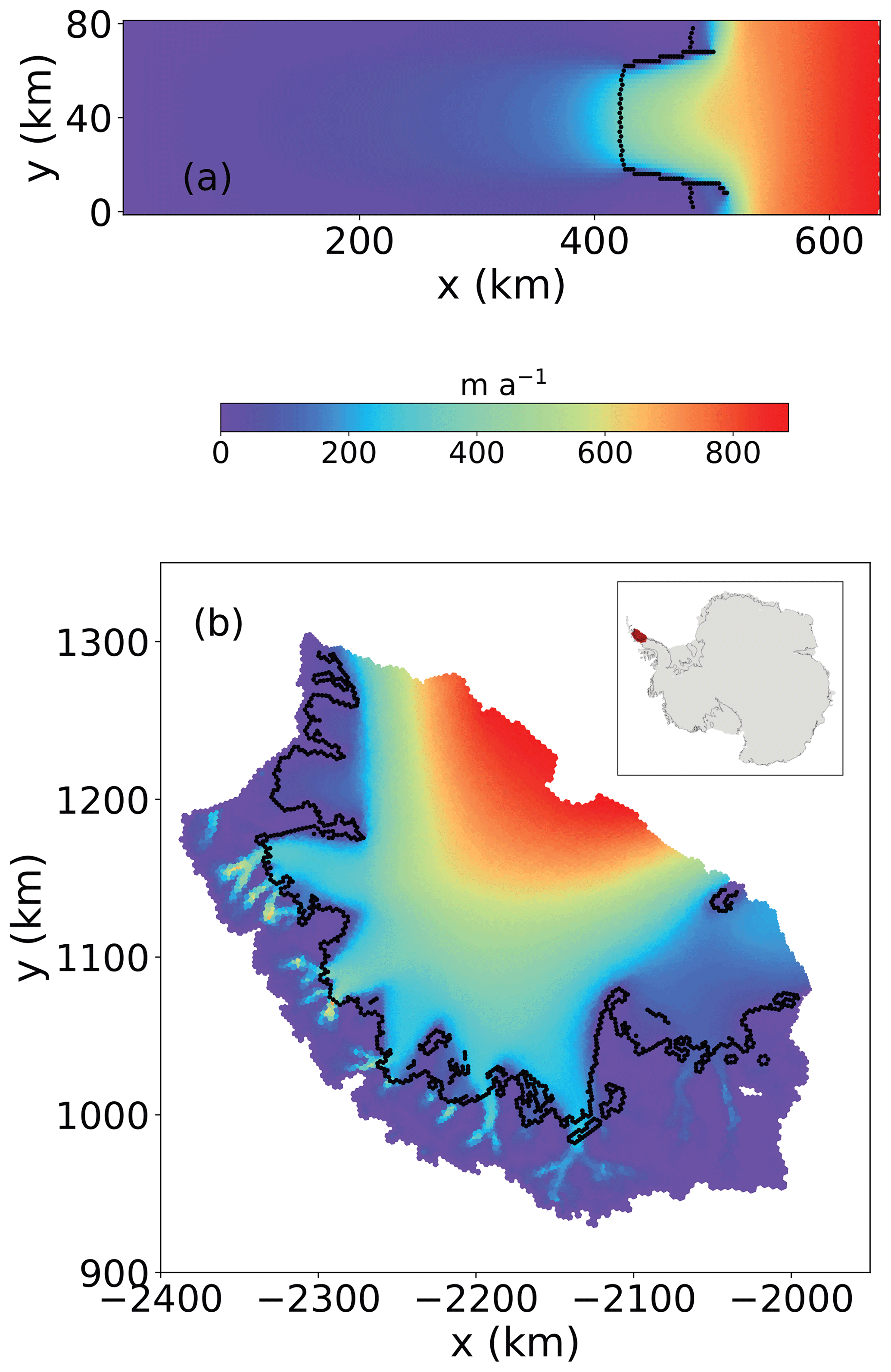
Figure 1(a) Plan view of surface speed for the MISMIP+ and (b) Larsen C Ice Shelf experimental domains. For the Larsen C domain, velocities have been optimized to match observations from Rignot et al. (2011). Black curves indicate the location of the grounding line. The location of the Larsen C Ice Shelf is shown as the shaded area in the inset in (b). A comparison of modeled and observed ice surface speed is provided in Fig. S1 in the Supplement.
2.1 Model description
We use the MPAS-Albany Land Ice model (MALI; Hoffman et al., 2018), which solves the three-dimensional, first-order approximation to the Stokes momentum balance for ice flow. Using the notation of Perego et al. (2012) and Tezaur et al. (2015a), this can be expressed as
where x and y are the horizontal coordinate vectors in a Cartesian reference frame, s(x,y) is the ice surface elevation, ρi represents the ice density, g is the acceleration due to gravity, and are given by
and
The “effective” ice viscosity, μe in Eq. (1), is given by
where γ is an ice stiffness factor; A is a temperature-dependent rate factor; n=3 is the power-law exponent; and the effective strain rate, , is defined as
where are the corresponding strain-rate components.
Under the first-order approximation to the Stokes equations, a stress-free upper surface can be enforced through
where n is the outward-pointing normal vector at the ice sheet's upper surface, . The lower surface is allowed to slide according to the continuity of basal tractions,
where β is a spatially variable friction coefficient, represent the viscous stresses, and u is the two-dimensional velocity vector (u, v). The field β is set to 0 beneath floating ice, and the basal traction is computed with the SEP3 method described in Seroussi et al. (2014). On lateral boundaries in contact with the ocean, the portion of the boundary above sea level is stress-free, while the portion below sea level feels the ocean hydrostatic pressure according to
where n is the outward-pointing normal vector to the lateral boundary (i.e., parallel to the (x,y) plane), ρw is the density of ocean water, and n1 and n2 are the x and y components of n. A more complete description of MALI, including the implementations for mass and energy conservation, can be found in Hoffman et al. (2018). Additional details on the momentum balance solver can be found in Tezaur et al. (2015a, b).
2.1.1 GLF computation
The grounding line (GL) is computed as the zero level set of , where H and b are the continuous, piecewise linear finite-element fields for the thickness and the bed topography, respectively, defined on a triangulation of the domain at hand. As a consequence, the GL is a piecewise linear curve, separating grounded ice (where ) from floating ice (where ). The flux F per unit width at a point on the GL is calculated as , where is the vertically averaged velocity, and nGL is the normal to the GL, pointing towards the floating-ice region. The integrated grounding-line flux, hereafter GLF, is the line integral of F along the GL, and it has units of cubic meters per year. We note that perturbations of the thickness far from the GL affect the GLF only through changes in the velocity field, whereas perturbations of the thickness at triangles intersecting the GL also directly affect ice thickness at the GL and, via the flotation condition, also possibly the position and length of the GL. We further note that ice rises in the model are also surrounded by grounding lines and require no special treatment.
2.2 Model configuration
We apply MALI to experiments on both idealized and realistic marine ice sheet geometries. For our idealized domain and model state, we start from the equilibrium initial conditions for the MISMIP+ experiments with a mesh resolution of about 2 km, as described in Asay-Davis et al. (2016). For our realistic domain, we use Antarctica's Larsen C Ice Shelf and its upstream catchment area. For the Larsen C domain, the model state is based on the optimization of the ice stiffness (γ in Eq. 4) and basal-friction (β in Eq. 7) coefficients in order to provide a best match between modeled and observed present-day velocities (Rignot et al., 2011) using adjoint-based methods discussed in Perego et al. (2014) and Hoffman et al. (2018). The domain geometry is based on Bedmap2 (Fretwell et al., 2013), and ice temperatures, which are used to determine the flow factor and held fixed for this study, are taken from Liefferinge and Pattyn (2013). Mesh resolution is 2 km at the grounding line and coarsens to 4 km near the calving front of the ice shelf and 5 km into the ice sheet interior. Following optimization to present-day velocities, the model is relaxed using a 100-year forward run, providing the initial conditions from which the Larsen C experiments are conducted (as discussed below). The domain and initial conditions were extracted from the Antarctica-wide configuration used by MALI for initMIP experiments (Hoffman et al., 2018; Seroussi et al., 2019). Both the MISMIP+ and Larsen C experiments use 10 vertical layers that are finest near the bed and coarsen towards the surface.
To explore the sensitivity of changes in GLF to small, localized changes in ice shelf thickness, we conduct perturbation experiments analogous to those of Reese et al. (2018). Using diagnostic model solutions, we calculate the instantaneous change in GLF for the idealized geometry and initial state provided by the MISMIP+ experiment (Asay-Davis et al., 2016). We then conduct similar experiments for Antarctica's Larsen C Ice Shelf using a realistic configuration and initial state. The geometries and ice speeds for MISMIP+ (steady-state) and Larsen C Ice Shelf (present-day) are shown in Fig. 1.
Our experiments are conducted in a manner similar to those of Reese et al. (2018). We perturb the coupled ice sheet–shelf system by decreasing the ice thickness uniformly by 1 m at ice shelf grid cells (note that perturbations are applied to Voronoi grid cells, which reside on the dual grid to the Delaunay triangulation used by the finite-element solver; every point of the Delaunay triangulation corresponds to a Voronoi cell center), after which we examine the instantaneous impact on kinematics and dynamics (discussed further below).
For both the MISMIP+ and Larsen C domains, the local ice shelf surface and basal elevations are adjusted following perturbations in order to maintain hydrostatic equilibrium. Lastly, for the MISMIP+ 2 km experiments, we note that, in order to save on computing costs, we only perturb the region of the ice shelf for which x<530 km (the area over which the ice shelf is laterally buttressed) and for which y>40 km (due to symmetry about the center line). We do, however, analyze the response to these perturbations over the entire model domain.
Similar to Reese et al. (2018), we define a GLF response number for our perturbation-based experiments,
where R is the change in the GLF due to a perturbation in the thickness at a single grid cell calculated over 1 year, and P is the local volume change associated with the perturbation. The subscript “rp” denotes the “response” from “perturbation” experiments. Note that both R and P have units of cubic meters so that Nrp is dimensionless.
Changes in GLF (quantified by Nrp) in response to a local change in ice shelf thickness are expected to occur via changes in ice shelf buttressing, which generally acts to resist the flow of ice across the grounding line. To quantify the local ice shelf buttressing capacity, we calculate a dimensionless buttressing number, Nb, analogous to that from Gudmundsson (2013) and Fürst et al. (2016),
where is a scalar measure of the stress normal to the surface defined by n. The two-dimensional stress tensor T is computed according to the shallow shelf approximation and is defined in Eq. (A6). N0 is the value of Tnn if the ice was removed up to the considered location and replaced with ocean water (or alternatively, the resistance provided by a static, neighboring column of floating ice at hydrostatic equilibrium) defined by
with ρi and ρw being the densities of ice and ocean water, respectively. For the MISMIP+ experiment, ρi is 918 kg m−3, and for the Larsen C experiment, ρi is 910 kg m−3. For both experiments, ρw=1028 kg m−3. We elaborate further on the calculation of the buttressing number in Appendix A. While Gudmundsson (2013) chose the unit vector n to be normal to the grounding line to define the “normal” buttressing number, Fürst et al. (2016) extended his definition to the ice shelf by examining Nb(n) for n along the ice flow direction and along the direction of the second principal stress. Here, we explore the connection between changes in grounding-line flux (quantified by Nrp), subshelf melting, and local buttressing on the ice shelf (quantified by Nb) corresponding to arbitrary n (in order to consider all possible relationships on the ice shelf). Note that we do not discuss the tangential buttressing number defined by Gudmundsson (2013); hereafter, we use “buttressing number” to refer exclusively to the “normal buttressing number”, as defined above.

Figure 2GLF number and buttressing number for each of the 730 perturbed grid cells in the MISMIP+ experiments. (a) The spatial distribution of the GLF response number, Nrp. (b–d) The spatial distribution of the buttressing number, Nb, corresponding to directions (b) np1, (c) np2, and (d) nf. Black dots indicate grid cells located along the grounding line. Here the color bars for (a)–(d) do not show the full data range. Note that the negative GLF numbers in panel (a) are due to the nonlinear impacts of changes in both ice thickness and velocity at the GL.
4.1 Correlation between buttressing and changes in GLF
A decrease in ice shelf buttressing tends to lead to an increase in GLF (e.g., Gagliardini et al., 2010; see also Fig. 2a) and intuitively we expect that the GLF should be relatively more sensitive to ice shelf thinning in regions of relatively larger buttressing. We aim to better understand and quantify the relationship between the local ice shelf buttressing “strength” in a given direction (characterized by Nb) and changes in GLF (characterized by Nrp). A reasonable hypothesis is that, for a given ice thickness perturbation, the resulting change in the GLF is proportional to the buttressing number at the perturbation location. In Fig. 2, we show the results from all (730) perturbation experiments for MISMIP+ and the corresponding Nrp and Nb values. We show values of Nb for three different directions, corresponding to the choice of n in Eq. (10): the first principal stress direction (np1), the second principal stress direction (np2), and the ice flow direction (nf). In the discussion below, we frequently refer to these three directions when discussing the buttressing number. In agreement with the findings of Fürst et al. (2016), the largest values for Nb occur when it is calculated in the np2 direction. While there appears to be a qualitatively reasonable spatial correlation between the magnitude of Nrp and Nb when the latter is calculated in the np2 and nf directions (and less so when calculated in the np1 direction), in Fig. 3 we show that there is no clear relationship between the response number Nrp and the buttressing number Nb calculated along any of these directions, at least for the case where we consider all points on the ice shelf.
In Fig. 4, we show correlations between the modeled value of Nrp and Nb where we ignore points meeting the following criteria: (i) points where the ice shelf becomes unconfined (x>480 km); (ii) points within two cells from the GL; (iii) points where shear stresses are large according to the metric
where σp1 and σp2 are the first and second principal normal stresses, respectively, and ms is the ratio of the maximum shear stress to the mean normal stress. For the case of (i), a good correlation between Nb and Nrp is not expected for unconfined flow where buttressing is insignificant (Van Der Veen, 2013). For the case of (ii), complications near the grounding line (e.g., grounding-line movement and geometry change associated with thickness perturbations, as noted in Sect. 2.1.1) may give incorrect GLF response numbers. For the case of (iii), we expect a relatively poor correlation between Nb and Nrp for locations where buttressing occurs primarily via lateral drag, which will be poorly captured by a stress metric (i.e., buttressing number) associated with a single direction. In a principal stress framework, shear stress is described by perpendicular normal stresses of opposite sign. Applying this metric means that we only evaluate correlations between Nb and Nrp for points where ms from Eq. (12) is <1 (i.e., where normal stress is dominant over shear stress; see also Fig. S2). When applying criteria (i)–(iii) above as a spatial filter, the number of points considered is reduced (Fig. 4a), and stronger correlations between Nrp and Nb emerge. In particular, a stronger correlation between Nrp and Nb occurs when Nb is calculated using np1 (Fig. 4b) or nf (Fig. 4d) relative to when using np2 (Fig. 4c).
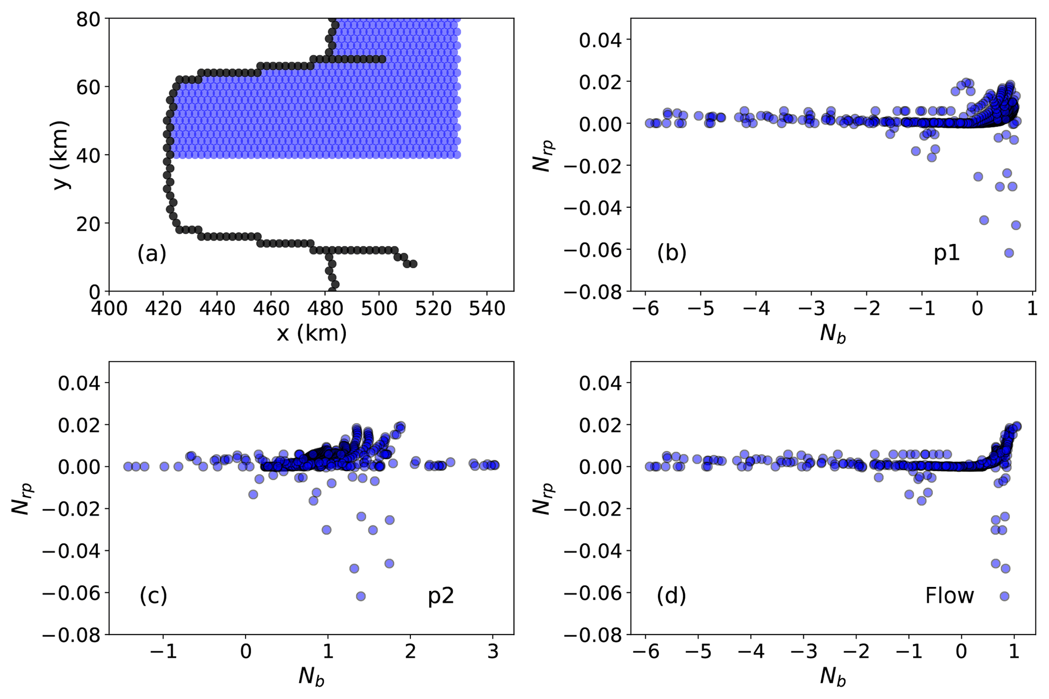
Figure 3(a) Blue dots represent the locations of all perturbation points analyzed (730) for the Nrp:Nb relation analysis. Black dots indicate grid cells located along the grounding line. (b–d) Modeled Nrp versus buttressing number Nb calculated along (b) np1, (c) np2, and (d) nf.
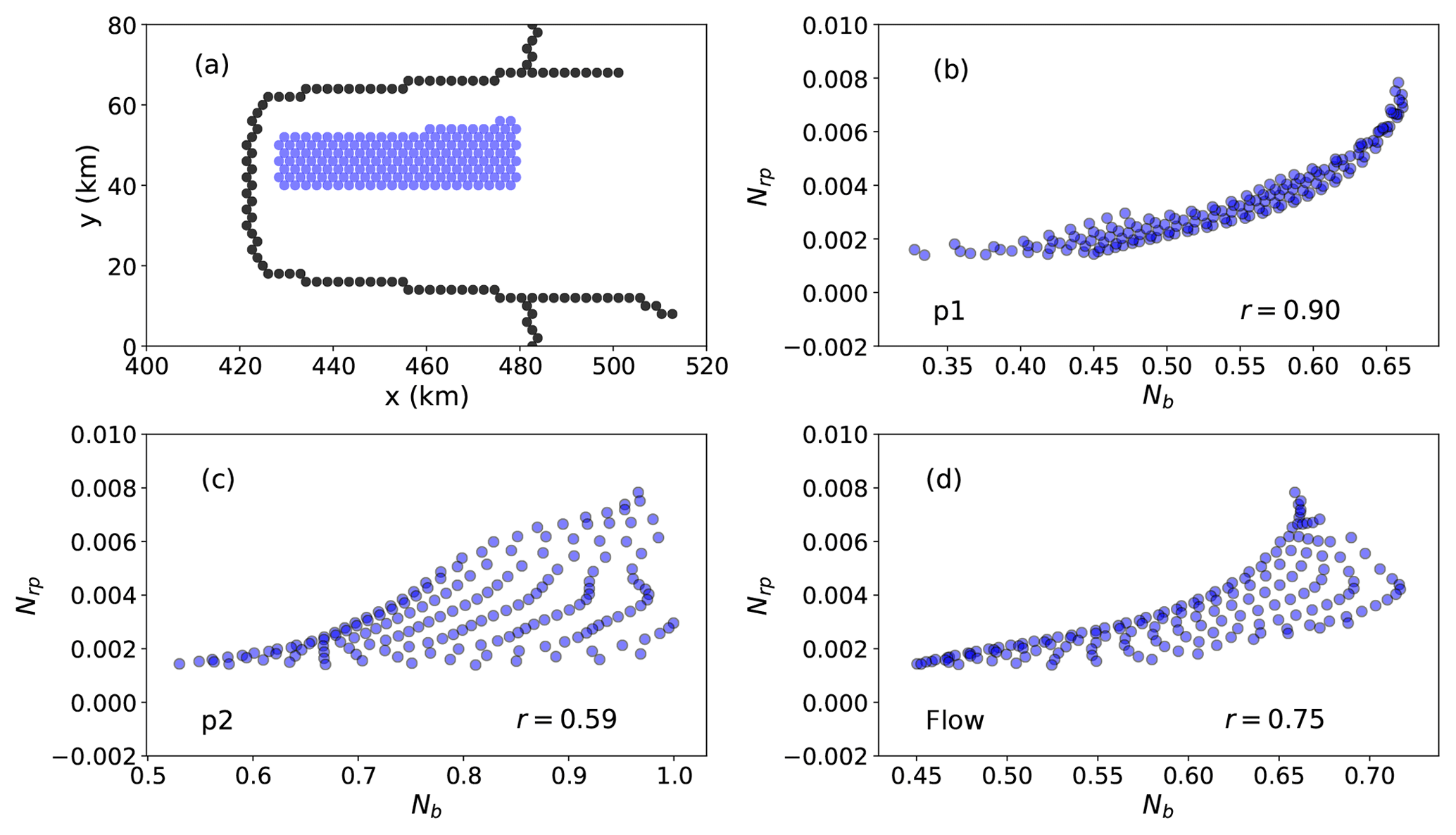
Figure 4(a) Blue dots represent the locations of all perturbation points analyzed (168) for the Nrp:Nb linear-regression analysis based on the filtering criteria discussed in Sect. 4.1. Black dots indicate grid cells located along the grounding line. (b–d) Modeled Nrp versus buttressing number Nb calculated along (b) np1, (c) np2, and (d) nf. The correlation coefficient for each modeled Nrp versus Nb is given by r.
4.2 Directional dependence of buttressing
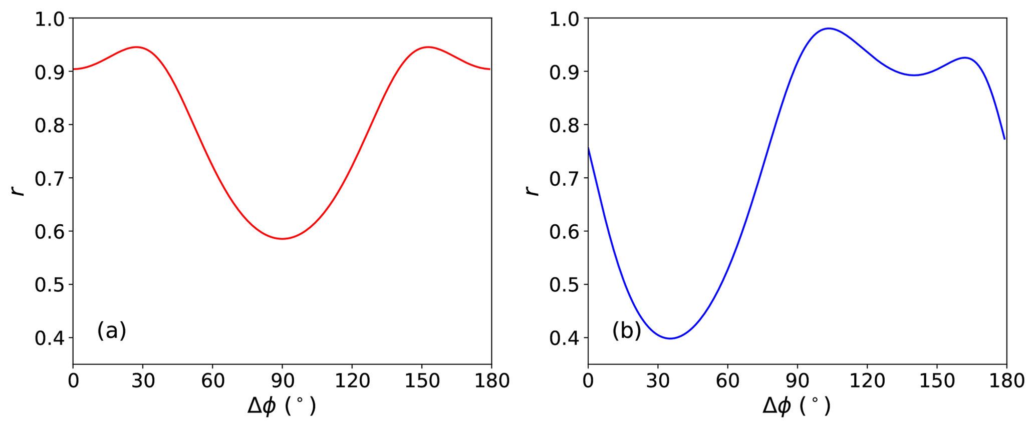
The buttressing number at any perturbation point depends on Tnn, which in turn depends on the chosen direction of the normal vector, n (Eq. 10). Fürst et al. (2016) calculated Nb using nf and np2 and chose the latter – the direction corresponding to the second principal stress (the maximum compressive stress or the least extensional stress) – to quantify the local value of “maximum buttressing” on an ice shelf. In Fig. 5a, we plot the linear-regression correlation coefficients (r) for the Nrp:Nb relationship, where the direction of n used in the calculation of Tnn varies continuously from Δϕ=0 to 180∘ relative to np1 (we also show how the buttressing number Nb varies as a function of direction in Fig. S3). We find large correlation coefficients (r>0.9) when Nb is aligned closely with np1 (Δϕ=0 or 180∘) and the smallest correlation coefficient (r<0.5) when Nb is aligned with np2 (). Similar conclusions can be reached when examining the variation in r with respect to the ice flow direction (Fig. 5b), where correlations are phase-shifted by approximately 50∘ counterclockwise relative to Fig. 5a. Clearly, the best correlation occurs along a direction somewhere between np1 and nf. Note that we do not see an exact match between Fig. 5a and b if we shift the angle by 50∘ because the angular difference between np1 and nf varies for the perturbation locations analyzed.
Fürst et al. (2016) posit that Nb(np2) provides a good local buttressing metric and chose it for identifying regions of maximum buttressing on an ice shelf with the goal of identifying “passive” ice that can be removed without tangibly affecting the remaining ice. While our results also show that buttressing is greatest in the direction of the second principal stress (which follows from the definitions of the second principal stress and the buttressing number; see also Fig. S3), we find that buttressing in this direction is not useful for predicting changes in GLF; compared to Nb(np2), Nb(np1) and Nb(nf) both show a better correlation with changes in GLF via local sub-ice-shelf melt perturbations. We discuss these differences further in Sect. 5.
4.3 Perturbation impacts: local, far-field, and integrated changes
We now look more carefully at thickness perturbations on the ice shelf in terms of their local, far-field, and integrated impacts on changes in geometry, velocity, stress, buttressing, and GLF.
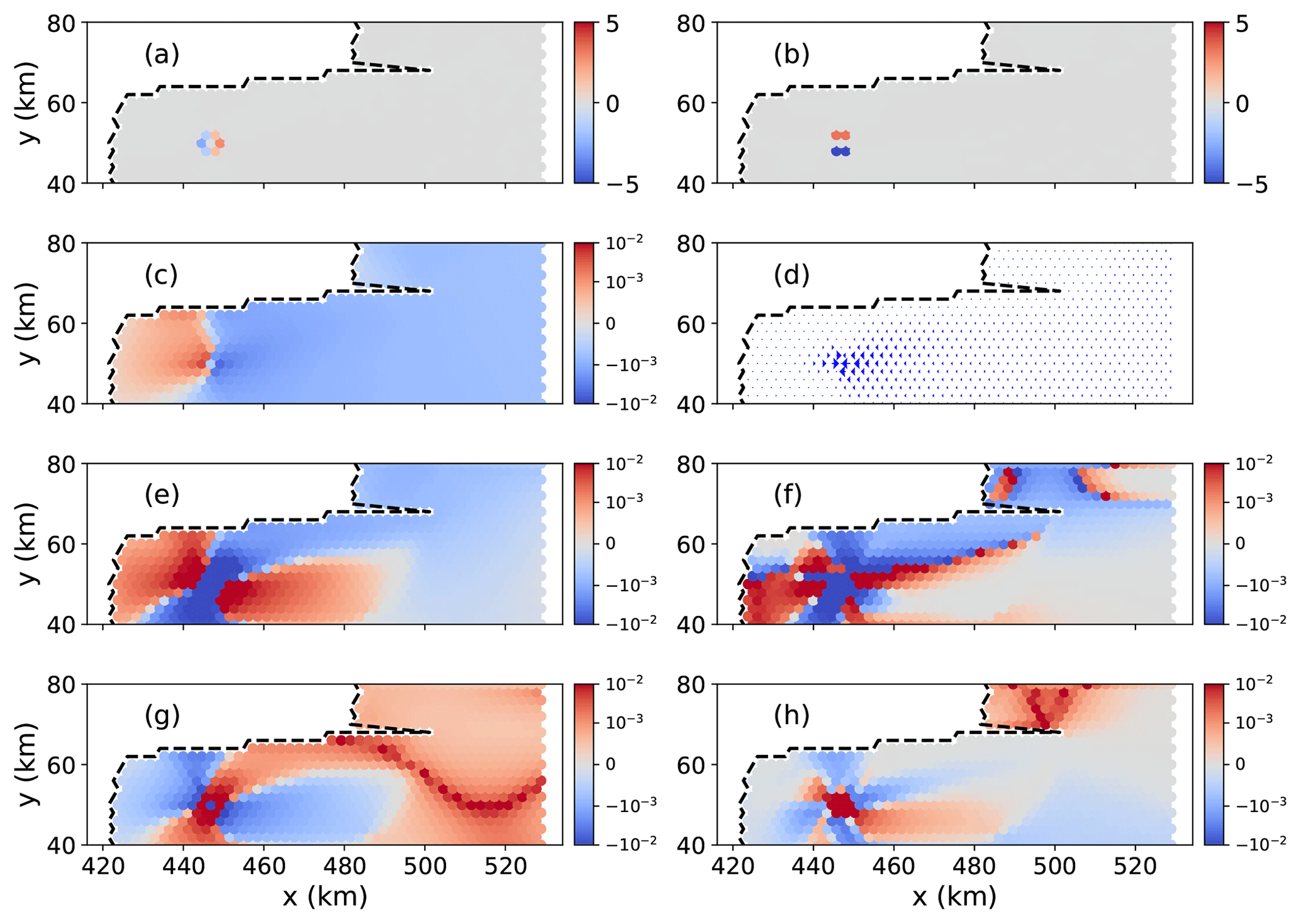
Figure 6An example of the local change (ratio, in percent) in (a) the ice thickness gradient in x, (b) ice thickness gradient in y, (c) ice speed, (d) ice velocity (relative), (e, f) principal strain rates, and (g, h) buttressing number following a local perturbation to the ice shelf thickness. In (e) and (g), changes (colors) are associated with the np1 direction, and for (f) and (h) changes are associated with the np2 direction.
4.3.1 Local perturbation impacts
Local thickness perturbations on the ice shelf alter the local ice thickness gradient; on the upstream side of the perturbation it becomes more negative, while on the downstream side it becomes less negative (Fig. 6a, b). These thickness gradient changes increase the ice speed immediately upstream from the perturbation and decrease it immediately downstream of the perturbation (Fig. 6c), resulting in anomalous flow convergence towards the perturbation location (Fig. 6d). The resulting impacts on the principal strain rates (and thus the principal stresses) are increased compression (or decreased extension) along both principal directions (Fig. 6e, f) and, via Eq. (10), a corresponding increase in the local value of Nb along both principal stress directions (Fig. 6g, h). These spatial patterns of change are robust for a number of different perturbation points on the ice shelf (see Figs. S4 and S5 in the Supplement).
An important caveat applies to the grid cell associated with the location of the perturbation itself, where a decrease in Nb is seen, sometimes for only the np1 direction but other times for both principal directions (Fig. S5). In Fig. 7, we quantify the local (at the perturbation location; Fig. 7a) and neighboring (immediately surrounding the perturbation location; Fig. 7b) changes in Nb for all of the points analyzed in Fig. 4 and for all possible directions. From Fig. 7, we make two conclusions: (1) the local change in Nb is generally more positive along the np2 direction (indicating a local increase in buttressing accompanying a thickness perturbation), and (2) the local and neighboring changes in buttressing are often inconsistent (i.e., a decrease in Nb at a particular grid cell coincides with an increase in Nb in the neighboring cells). The first conclusion would seem to argue against using Nb(np2) for quantifying local changes in buttressing in terms of their broader impacts on GLF (because, surprisingly, local thinning perturbations are more likely to indicate a local increase in buttressing along the np2 direction). The second conclusion suggests that analysis over wider spatial scales may be necessary for a consistent understanding of how local ice shelf perturbations impact GLF.
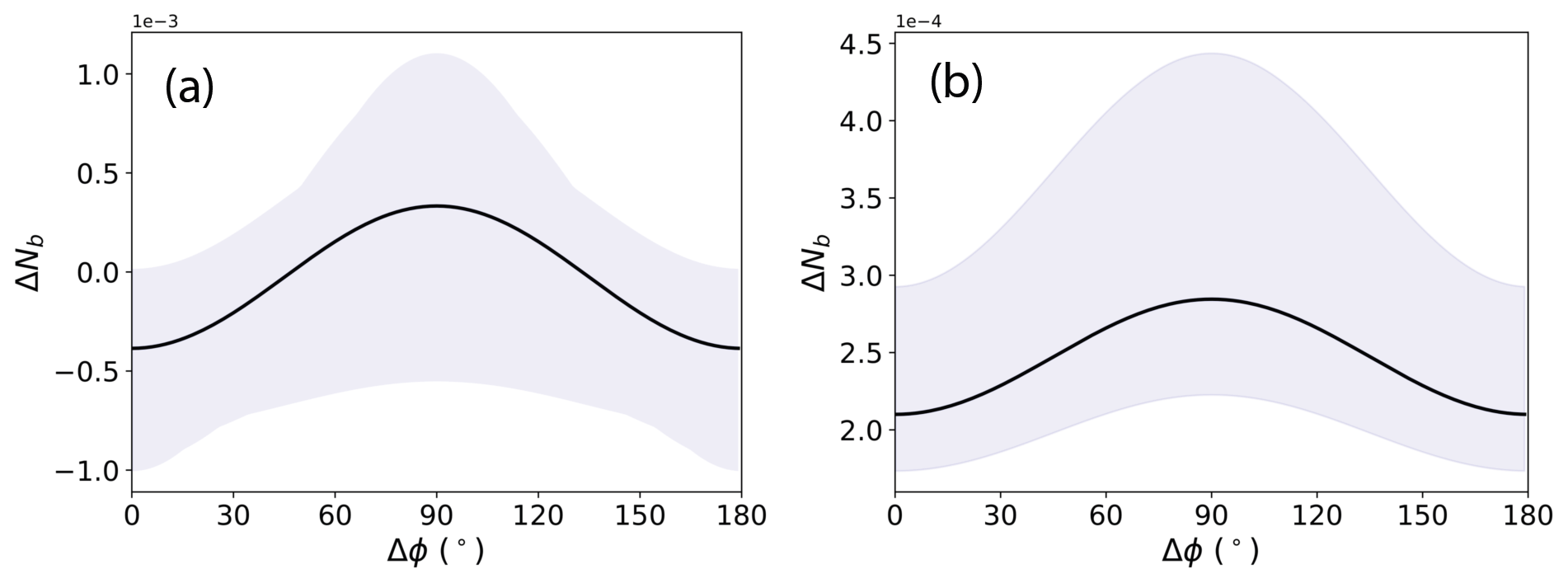
Figure 7The change in buttressing number, ΔNb, at and near to ice shelf thickness perturbations. In (a), the change at the perturbation location is shown, and in (b) the mean change in all immediately neighboring cells is shown. Changes in buttressing are calculated along the direction Δϕ, rotated counterclockwise relative to the np1 direction. The points analyzed include those in Fig. 4a, which are shown as the shaded area, with the solid curve representing their mean value.
4.3.2 Far-field perturbation impacts
Away from the immediate vicinity of ice shelf thickness perturbations (i.e., beyond the grid cell where perturbations are applied and its immediate neighbors), the resulting changes are more uniform and easier to interpret. The broader pattern of increased ice speed upstream from a perturbation location can be seen to extend spatially and diffuse with increased distance (Fig. 6c). A similar pattern can be observed with respect to changes in principal strain rates and buttressing, at least for the np1 direction (Fig. 6e and g), where a wide swath of increased extension and decreased local buttressing (as quantified by reductions in Nb(np1)) coincides with the region of increased ice speed extending upstream to the grounding line. This implied causality – a reduction in buttressing on the shelf leads to an increase in GLF upstream – is consistent with our understanding of ice shelf buttressing. Importantly, we note that a similar understanding based on changes in the np2 direction (Fig. 6f and h) is much less straightforward due to more complicated spatial patterns and no obvious consistency between reductions in Nb(np2) and the increases in ice speed that would lead to a corresponding increase in GLF. This interpretation of the far-field effects of local ice shelf perturbations is consistent when perturbations are applied at a number of different locations on the ice shelf (see Figs. S4 and S5 in the Supplement).
A reasonable hypothesis is that the apparent correlation between Nb(np1) and Nrp in Fig. 4b arises because of the connection, discussed above, between local thickness perturbations, far-field changes in principal stresses and buttressing along the np1 direction, and increases in ice speed upstream of the perturbation. Similarly, the lack of such a clear connection for local perturbations and principal stresses and buttressing along the np2 direction may account for the relatively poorer correlation between Nb(np2) and Nrp shown in Fig. 4c. Next, we explore how these far-field changes are expressed at the grounding line.
4.3.3 Perturbation impacts on buttressing and ice flux at the grounding line
To understand how local perturbations in ice shelf thickness impact GLF, we now examine changes in the buttressing number and ice speed at and normal to the grounding line. To quantify this relationship, we define Υgl as
where and and with the subscripts p and c denoting the “perturbed” and “control” (i.e., initial) model states, respectively. ΔNb and Δu denote vectors of the changes in the buttressing number and ice speed normal to the GL, respectively, for all GL cells along the main trunk of the ice stream (red points in Fig. 8). Υgl, a correlation coefficient, is an integrated measure of the consistency between the magnitude and the sign of the change in buttressing number and ice speed between the control and perturbation experiments, with cov and s representing the covariance and the standard deviation, respectively.
By plotting values of Υgl mapped to their respective perturbation locations on the ice shelf (Fig. 8), we show there is generally a negative correlation between speed and buttressing at the GL: in response to a thickness perturbation on the ice shelf, buttressing decreases and speed (and hence flux) across the GL increases, in line with our general understanding of buttressing. In Fig. 8a, we show a reference case for which Tnn in Eq. (10) – and hence in Eq. 13 – is calculated normal to the grounding line. In this case, the Nb values in Eq. 13 are calculated along the GL as defined by Gudmundsson (2013; Υgl=Υgl(ngl), where ngl is the direction normal to the grounding line). In Fig. 8b and c, we show Υgl(np1) and Υgl(np2), respectively. As expected, the correlation is strongly negative for Υgl(ngl) (Fig. 8a), and we find that Υgl(np1) is a close match (Fig. 8b). While much of the shelf under consideration also shows a negative correlation for Υgl(np2), the correlations are generally weaker, and there are regions near the center of the shelf and closer to the grounding line where the correlation switches sign, implying an increase in buttressing (as calculated in that direction) accompanying an increase in GLF (Fig. 8c).
In addition to the results for the three discrete normal directions discussed above, a continuous analysis of Υgl as a function of the normal stress direction is shown in Fig. 9, where we plot Υgl at each perturbation point and for all directions in the range of Δϕ=0–180∘ relative to np1. This correlation is generally negative and stronger for buttressing numbers calculated near the np1 direction (Δϕ closer to 0 or 180∘) and weaker (or even strongly positive) approaching the np2 direction. This analysis connects the local perturbations and far-field impacts described above with changes in integrated GLF, providing a further means for understanding the correlation between Nb(np1) and Nrp in Fig. 4b.
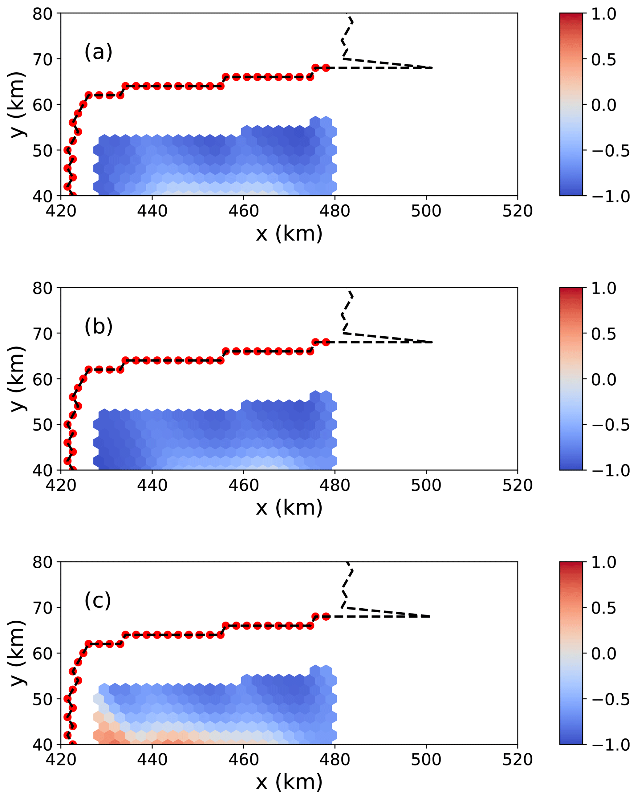
Figure 8Spatial distribution of the correlation coefficient Υgl from Eq. (13) over the MISMIP+ domain for buttressing number changes calculated parallel to (a) ngl, (b) np1, and (c) np2 (colors). Υgl is a measure of the correlation between changes in buttressing number and ice speed along the grounding line. The dashed black line represents the grounding line, and the red dots indicate the area of the grounding line for which values of Υgl are calculated for each perturbation on the ice shelf, as shown in Fig. 4a.

Figure 9Correlation between the change in buttressing number and the change in ice speed across the grounding line (i.e., Υgl from Eq. 13) for the entire MISMIP+ grounding line. The horizontal axis shows how Υgl varies as a function of the direction n used to define the normal stress, rotated counterclockwise from np1 by Δϕ. Values from the maps in Fig. 8a and b plot at Δϕ values of 0 and 90∘, respectively. Thus, the shaded blue region represents all possible maps for all possible values of buttressing direction. The thick black curve represents the mean value of Υgl for any given map.
4.3.4 Summary of local versus integrated impacts of ice shelf perturbations
The changes in ice speed and buttressing at the grounding line quantified by Figs. 8 and 9 must be the result of perturbations initiated on the ice shelf that have propagated (here, instantaneously) to the grounding line, where increases in speed are associated with increased extension along np1 and, according to Eq. (10), decreased buttressing associated with the np1 direction. Intuitively, these increases in ice speed at the grounding line must be triggered by the loss of buttressing on the shelf, initiated here via small and highly localized ice thickness (thinning) perturbations. As shown and argued above, however, it is difficult to understand the integrated impacts of these perturbations on GLF based on changes in locally derived quantities alone, in particular the locally derived buttressing number, Nb. One would come to very different conclusions regarding how a perturbation impacts local buttressing depending on both the spatial scale of the area around a perturbation being examined and the principal direction used for calculating Nb (e.g., Fig. 7a and b). Over wider spatial scales, however, we do find consistency between the impacts of local perturbations on geometry, stresses, local buttressing, ice speed, and changes in GLF (Figs. 6, 8, 9). While we hypothesize that it is this consistency that lies behind the apparent correlation between Nb and Nrp in Fig. 4b, we still lack the detailed physical understanding behind that correlation that would be required for us to apply it with confidence.
Further, we show in the Supplement and Table S1 that the correlation between Nb and Nrp may be spurious, perhaps due to correlations with some other common variable. More importantly, in the next section we show that this tenuous correlation between Nb and Nrp breaks down almost entirely when applied to a realistic ice shelf.
4.4 Application to Larsen C Ice Shelf
We apply a similar set of analyses, as discussed above for the MISMIP+ domain, to a realistic Larsen C Ice Shelf domain. For this domain, with complex geometry and spatially variable ice temperature (and associated ice rigidity), the relationship between Nb(np1) and Nrp becomes much weaker relative to that for the MISMIP+ domain. Figure 10 shows that using the shear metric ms (Eq. 12) to filter locations reduces the scatter between Nb(np1) and Nrp. However, even when retaining only points with low shear contributions, the relationship is nonlinear without a clear functional form. Furthermore, restricting analysis to the low-shear regions where the relationship is stronger excludes the majority of the ice shelf, including most of the regions where the GLF response number is large (see also Fig. 13a below). We find a similar result when coarsening the analysis to use 20 km×20 km boxes for the analysis, as was done for the Nrp calculations performed by Reese et al. (2018); a strong correlation exists for only a small area near the center of the ice shelf (Fig. S6). Even weaker relationships are found for the np2 and nf directions. Thus, while there clearly is some link between Nb(np1) and Nrp for a realistic ice shelf, it is far too tenuous to be used in a predictive way and likely differs across and between ice shelves.
Overall, for a realistic ice shelf like Larsen C with a complex geometry and flow field, we find it even more difficult to demonstrate robust relationships between the local ice shelf buttressing number and changes in GLF. This is, at least in part, likely due to the fact that, for more complex and realistic domains, there is no dominant direction of buttressing controlling ice flux across the grounding line. These findings further diminish our confidence in using locally derived buttressing numbers for assessing the sensitivity of GLF to changes in the ice shelf. For this reason, we explore an alternative and more robust method for quantifying how ice shelf thickness perturbations affect flux at the grounding line.
4.5 Adjoint sensitivity
While our goal throughout this study has been to find a simple and robust metric for diagnosing GLF sensitivity to ice shelf thickness perturbations, the challenges and complications discussed above suggest that this may not be possible. This motivates our investigation of a wholly different approach, which provides a GLF sensitivity map analogous to that from Reese et al. (2018) instead of seeking a simple buttressing number indicator to predict the GLF sensitivity. But rather than computing the GLF change due to a perturbation applied individually at each of n model grid cells (thus requiring n diagnostic solves), we use an adjoint-based method that allows for the computation of the sensitivity at all n grid cells simultaneously at the cost of a single adjoint model solution. Briefly, this method involves the solution of an auxiliary linear system (the adjoint system) to compute the so-called Lagrange multiplier, a variable with the same dimensions as the forward-model solution for the ice velocity. Here, the matrix associated with the system is the transpose of the Jacobian of the first-order approximation to the Stokes flow model (Perego et al., 2012). In addition, the adjoint method requires computation of the partial derivatives of the first-order model residual and the GLF with respect to the velocity solution and the ice thickness. Here, we compute the Jacobian and all the necessary derivatives using automatic differentiation (Tezaur et al., 2015a). Additional details of the adjoint-based method and calculations are given in Appendix C.
A similar approach has been proposed by Goldberg et al. (2019). That work primarily assessed the adjoint sensitivity of the volume above floatation with respect to sub-ice-shelf melting of the Dotson and Crosson ice shelves in West Antarctica. In contrast to our approach, Goldberg et al. (2019) compute transient sensitivities because their quantity of interest (volume above floatation) is time-dependent. The adjoint-based sensitivity has units of volume flux per year per meter of ice thickness perturbation (m2 yr−1). We nondimensionalize this value, dividing it by the area of the perturbed cell and multiplying it by the 1-year period over which we consider the perturbation, so that it is dimensionless and comparable to Nrp, and we refer to it as Nra (where the subscript “a” is for “adjoint”). In Figs. 11 and 12, we demonstrate the application of this method to the MISMIP+ and Larsen C domains by comparing GLF sensitivities deduced from 730 and 1000 points (i.e., from the respective perturbation experiments discussed above for the MISMIP+ and Larsen C domains, respectively) with those deduced from a single adjoint-based solution. The comparison demonstrates that the two approaches provide a near-exact match.
As might be expected based on the discussion above, the two methods disagree in regions very close to the grounding line (see Fig. 13c). This discrepancy is likely a consequence of large nonlinearities near the grounding line, as suggested by the fact that the agreement between the two methods improves as the size of the perturbation decreases (from 10 to 0.001 m; see Fig. 13), the only change being the magnitude of the applied perturbation. This might be exacerbated by the sliding law adopted in this work, which results in abrupt changes in the basal traction across the grounding line. Other sliding laws, e.g., Brondex et al. (2017), allow for a smoother transition at the grounding line and might mitigate this problem. We also note that some isolated cells adjacent to the grounding line exhibit negative sensitivities (a decrease in ice flux following a decrease in ice thickness) opposite those exhibited by the rest of the ice shelf. We attribute these to partially grounded cells, for which the sensitivity may be more akin to that expected for grounded ice (i.e., a direct relationship between ice thickness and ice flux).
The adjoint sensitivity map represents a linearization of the GLF response to thickness perturbations. As long as the perturbations are small enough, one can approximate the GLF response by multiplying the sensitivity map by the thickness perturbation. Comparison of Nra and Nrp for different perturbation sizes (Fig. 13) suggests that this is reasonable for perturbations on the order of <10 m for points on the ice shelf that are not too close to the GL. At the same time care should be taken when interpreting the sensitivities – based on either the perturbation- or adjoint-based methods – in the vicinity of grounding lines. This is especially important when considering that the near-grounding-line region is also that with the largest sensitivities (Figs. 11a and 12a). Because these sensitivities may be inaccurate, they provide an argument for applying high spatial resolution near the grounding line; coarse resolution near the grounding line will extend the region over which inaccurate sensitivities may be assessed. More accurately assessing the sensitivities near the grounding line may require the application of perturbations with both magnitudes and spatial scales that are more realistic than the infinitesimal, highly localized perturbations explored here.
The adjoint method provides sensitivity maps over the entire ice shelf, including around islands, promontories, and along the grounding line itself, which is generally the part of the ice shelf where the GLF is the most sensitive to thickness perturbations (see, e.g., Figs. 11a and 12a and Fig. 1 in Reese et al., 2018). Thus, despite the added complexity in its computation, the adjoint-based method provides significant advantages over the simpler perturbation-based analysis methods discussed above.
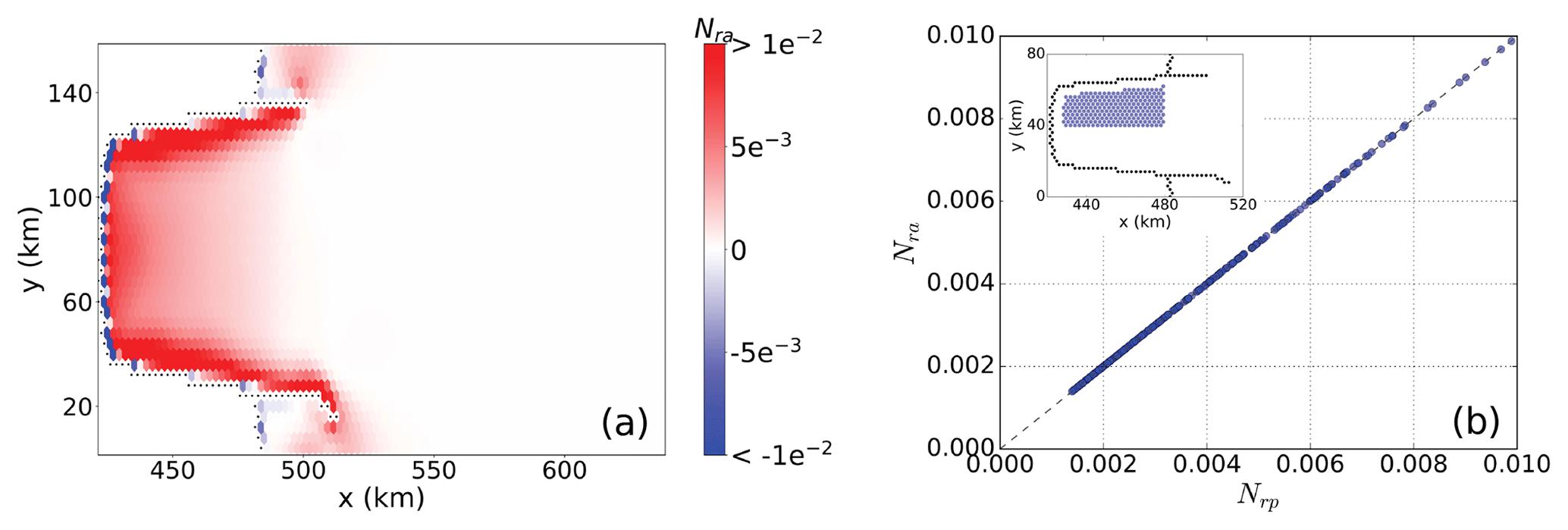
Figure 11(a) Grounding-line flux sensitivity for the MISMIP+ domain derived from the adjoint model approach. (b) Perturbation- (Nrp; x axis) versus adjoint-based (Nra; y axis) sensitivities plotted against one another (perturbation locations are shown by circles in the inset, where the grounding-line grid cells are shown by the black dots.)
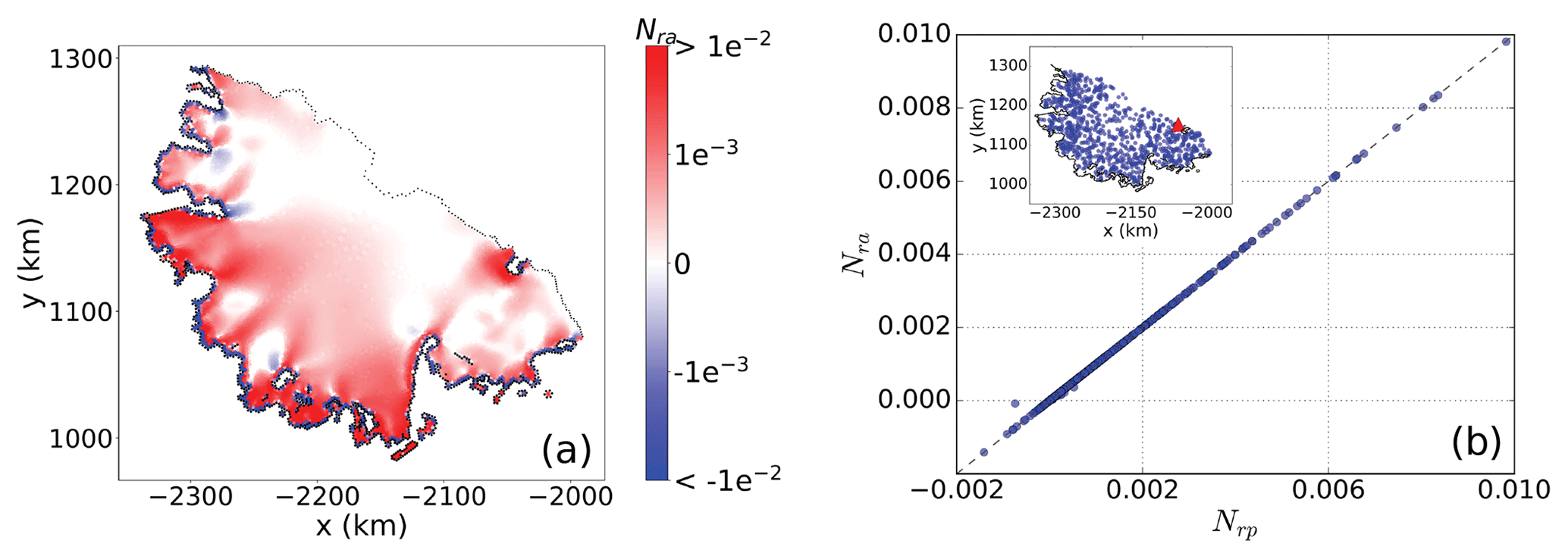
Figure 12(a) Grounding-line flux sensitivity for the Larsen C domain derived from the adjoint model approach. (b) Perturbation- (Nrp; x axis) versus adjoint-based (Nra; y axis) sensitivities plotted against one another (perturbation locations are shown by circles in the inset, where the one outlier in b is at the calving front – red triangle – and the grounding-line grid cells in map view are shown by the black line.)

Figure 13Comparisons between perturbation- and adjoint-based sensitivities (Nrp and Nra, respectively) for ice thickness perturbations of (a) 0.001, (b) 0.01, (c) 1, and (d) 10 m for perturbation points near the grounding line (<3 km), indicated by the dots on the inset map in (a). Red dots represent grid cells next to the grounding line, and blue dots represent grid cells on the ice shelf proper.
The current interest in better understanding the controls on the MISI is due to the potential for future (and possibly present-day, ongoing) unstable retreat of the West Antarctic ice sheet (e.g., Joughin et al., 2014; Hulbe, 2017; Konrad et al., 2018). Because a loss of ice shelf buttressing is a primary cause of increased GLF (and thus an indirect control on the MISI), recent attention has been focused on better understanding the sensitivity of ice shelf buttressing to increases in iceberg calving and sub-ice-shelf melting. In this study, we have attempted to better characterize and quantify how local thickness perturbations on ice shelves – a proxy for local thinning due to increased sub-ice-shelf melting – impact ice shelf buttressing and GLF.
Two previous approaches for assessing GLF sensitivity to changes in ice shelf buttressing – the flux response number (Nrp) and the buttressing number (Nb) – show significant correlations with one another only over regions with a relatively small shear component. In addition, this correlation is highly dependent on the direction chosen to define buttressing. Specifically, we find that the choice of the normal vector used when calculating Nb dictates whether the correlation between Nrp and Nb is significant or not. Here, for both idealized and realistic ice shelf domains, we find a weak correlation between Nrp and Nb when the normal stress used in calculating the buttressing number corresponds to the second principal stress direction (np2). The correlation is stronger (though sometimes still fairly weak) when Nb is calculated in the direction associated with the first principal stress (np1) or the ice flow (nf).
These findings appear at odds with the interpretation from previous efforts of Fürst et al. (2016), who argue that buttressing provided by an ice shelf is best quantified by Nb calculated in the direction of np2. The seeming contradiction may be partially rectified by considering the different foci of Fürst et al. (2016) versus the present work: while Fürst et al. (2016) primarily focused on how the removal of passive shelf ice (identified by Nb(np2)) impacted ice shelf dynamics, as quantified by the change in ice flux across the calving front, our focus is specifically on how localized ice shelf thickness perturbations impact the change in ice flux across the grounding line.1 While changes in calving flux are likely to impact the amount of buttressing provided by an ice shelf, they do not directly contribute to changes in sea level. For this reason, changes in GLF are arguably the more important metric to consider when assessing the impacts of changes in ice shelf buttressing.
Of significant concern in applying the apparent correlation between Nrp and Nb (relatively difficult and easy quantities to calculate, respectively) is the lack of a clear physical connection between local changes in buttressing on the ice shelf and integrated changes in flux at the grounding line. Here, we show that localized thinning on the shelf can lead to either increases or decreases in the local buttressing metric Nb, depending on both the direction of the normal stress chosen and the neighborhood over which these changes are estimated. Yet these same perturbations consistently result in a net decrease in buttressing and consequently a net increase in grounding-line flux. While this can often be understood through the detailed spatial analysis of the impacts for a single perturbation (e.g., Sect. 4.3 and Fig. 6), this finding suggests that local evaluations of buttressing on the ice shelf alone should be interpreted with extreme caution as they may not be physically meaningful with respect to understanding overall changes in GLF. It is also possible that the correlations we find between Nrp and Nb are fortuitous or spurious, giving us further pause in attempting to apply them in a predictive sense.
Practically speaking, however, these nuances may be irrelevant; when realistic and complex ice shelf geometries are considered, clear and robust relationships between Nrp and Nb are elusive or absent. For the Larsen C domain considered here, strong, positive correlations are only found to exist over a small, isolated region near the center of the ice shelf; proximity to the grounding line, the calving front, complex coastlines, islands, and promontories serves to degrade these correlations significantly, reducing the utility of the buttressing number as a simple metric for diagnosing GLF sensitivity on real ice shelves. Further, defining “proximity” – and hence an adequate distance away from these complicating features or other filtering metrics – appears to be largely arbitrary. Lastly, it is precisely these more complex regions, close to the ice shelf grounding lines, where sub-ice-shelf thinning will result in the largest impact on changes in GLF (as demonstrated in Figs. 11a and 12a).
Considering these complexities, we propose that assessing GLF sensitivities for real ice shelves requires an approach analogous to the perturbation method used by Reese et al. (2018). Due to the computational costs and the experimental design complexity associated with the perturbation-based method, we propose that an adjoint-based method is the more efficient way for assessing GLF sensitivity to changes in buttressing resulting from changes in sub-ice-shelf melting. Future work should focus on applying these methods to assessing the sensitivities of real ice shelves based on observed or modeled patterns of sub-ice-shelf melting and assessing how these sensitivities change in time along with the evolution of the coupled ocean-and-ice shelf system.
At the calving front, the stress balance is given by
where σ is the Cauchy stress tensor, n is the unit normal vector pointing horizontally away from the calving front, and pw is the water pressure against the calving front provided by the ocean. In a Cartesian reference frame, this gives two equations for the stress balance in the two horizontal directions:
Expressing the Cauchy stress as the sum of the deviatoric stress and the isotropic pressure () and assuming that the vertical normal stress σzz is hydrostatic gives
Combining Eqs. (A2) and (A3) gives
On ice shelves, the left-hand terms in Eq. (A4) can be taken as invariant in the z direction, and by vertically averaging (A4) we obtain
If we define the two-dimensional stress tensor T as
we can write Eq. (A5) as
where is the average pressure exerted by the ocean against the calving front (as defined in Eq. 11). The buttressing number, defined by
is thus a scalar measure of the balance between this average ocean pressure and internal stress within the ice shelf. For the case of Nb=0, these two exactly balance such that stresses within the ice shelf do not further restrain or compel the ice flow.
Thomas (1979) defines the concept of “back pressure” or “back stress”, which was formalized by Thomas and MacAyeal (1982) and MacAyeal (1987) as the stress provided by lateral shearing and compression around ice rises in excess of that of a freely spreading ice shelf. While the concept was conceived as applying along the grounding line (Thomas, 1979; MacAyeal, 1987), it was extended to any material surface within an ice shelf (Thomas and MacAyeal, 1982; MacAyeal, 1987). This older concept of a normal pressure characterizing downstream ice shelf conditions is reminiscent of the buttressing number defined by Gudmundsson (2013) and extended by Fürst et al. (2016) as the buttressing number (Nb), defined in Eq. A8 (and Eq. 10). Here we show that back stress is equivalent to Nb calculated in the along-flow direction and normalized by the hydrostatic stress.
We follow Van Der Veen (2013) and Cuffey and Paterson (2010) and define back force, FB, as the difference between the driving force of an ice shelf, FD, and the resistive force from longitudinal stretching, FL:
The driving force for an ice shelf is
and the longitudinal stretching force for a freely spreading ice shelf is
where and are the along-flow and across-flow deviatoric stresses, respectively. Therefore, we obtain
according to Eq. (A6), where is the along-flow stress in the along-flow coordinate system, equivalent to the normal stress along the flow direction, nf⋅Tnf, in the x,y coordinate system. To obtain the back stress, Bs, as a stress normal to a vertically oriented material surface, divide Eq. (B1) by thickness (force per unit width divided by thickness):
However, if we observe that the driving stress of an ice shelf is the hydrostatic stress, N0 (Eq. 11), multiplied by the thickness,
combined with Eq. (B4), we can rewrite the back stress as
Dividing (normalizing) by N0 then gives
which is analogous to Eq. (A8) above.
This result, while fairly straightforward to arrive at, brings the current concept of “buttressing” at the grounding line (as defined by Gudmundsson, 2013, and extended to “buttressing number” on the ice shelf by Fürst et al., 2016) together with the much older concept of ice shelf “back stress” (e.g., Thomas and MacAyeal, 1982).
The adjoint method is often used to compute the derivative (or “sensitivity”) of some quantity (here, the GLF) that depends on the solution of a partial differential equation with respect to parameters (here, the ice thickness; see, e.g., Gunzburger, 2012). It is particularly effective when the number of parameters is large because it only requires the solution of an additional linear system, independently of the number of parameters. In the discrete case, the GLF is a function of the ice speed vector, u, and the ice thickness vector, H. Using the chain rule, we compute the total derivative of the GLF with respect to the ice thickness as
Here denotes the matrix with components . Similarly and are row vectors with components and , respectively. The first term on the right-hand side of Eq. (C1) accounts for the fact that a perturbation of the thickness would affect the ice velocity, which in turn would affect the GLF. The second term on the right-hand side of Eq. (C1) accounts for changes in the GLF directly due to changes in thickness and is nonzero only when the thickness is perturbed at triangles intersecting the GL. In this case, a thickness perturbation would affect the position and length of the GL and the thickness of the ice at the GL.
In order to compute , we write the finite-element discretization (Tezaur et al., 2015b) of the flow model (Eq. 1) in the residual form and differentiate with respect to H:
Here is a square matrix referred to as the Jacobian. It follows that is a solution of
Note that this corresponds to solving many linear systems, one for each column of (i.e., for each entry of the ice thickness vector). We can then compute the sensitivity as
The main idea of the adjoint-based method is to introduce an auxiliary vector variable λ for solution of the adjoint system
and then to compute the sensitivity as
Equations (C4) and (C6) are equivalent, but the latter has the advantage of requiring the solution of a single linear system given by Eq. (C5). In MALI, the Jacobian and the other derivatives, ,, and , are computed using automatic differentiation, a technique that allows for exact calculation of derivatives up to machine precision. For automatic differentiation, MALI relies on the Trilinos Sacado package (Phipps and Pawlowski, 2012). As a final remark, we note that the term requires the computation of shape derivatives because a change in thickness affects the geometry of the problem. This is not the case for two-dimensional, depth-integrated flow models (e.g., as in Goldberg et al., 2019) or when using a sigma coordinate to discretize the vertical dimension.
We conclude this section by pointing out that the sensitivity depends on the local refinement of the mesh, and it vanishes as the mesh is refined. This is particularly important in the case of nonuniform meshes because the sensitivity map would strongly depend on the refinement. In order to overcome this issue, it is advisable to scale the sensitivity by premultiplying it by the inverse of the mass matrix (in a finite-element context) or, similarly, dividing it point-wise by the measure (area) of the dual cells, as done in this paper to compute Nra. We refer to Li et al. (2017), Sect. 6, for an in-depth analysis in the optimization context.
The code of the ice sheet model (MALI) can be found here: https://github.com/MPAS-Dev/MPAS-Model/releases (last access: 6 October 2020) (V6.0) (Duda, 2019). The datasets used in this paper can be found in https://doi.org/10.5281/zenodo.3872586 (Zhang et al., 2020).
The supplement related to this article is available online at: https://doi.org/10.5194/tc-14-3407-2020-supplement.
TZ and SFP initiated the study with input from MJH, MP, and XAD. TZ conducted the diagnostic simulations with MALI and the majority of the analysis. The adjoint experiments were conducted by MP. All authors contributed to the writing of the paper.
The authors declare that they have no conflict of interest.
Sandia National Laboratories is a multimission laboratory managed and operated by National Technology and Engineering Solutions of Sandia, LLC., a wholly owned subsidiary of Honeywell International, Inc., for the US Department of Energy's National Nuclear Security Administration under contract DE-NA-0003525.
This paper describes objective technical results and analysis. Any subjective views or opinions that might be expressed in the paper do not necessarily represent the views of the US Department of Energy or the United States Government.
The authors thank Hilmar Gudmundsson, two anonymous reviewers, and the editor, Olivier Gagliardini, for comments and suggestions that significantly improved the manuscript. This research used resources of the National Energy Research Scientific Computing Center, a DOE Office of Science user facility supported by the Office of Science of the US Department of Energy under contract no. DE-AC02-05CH11231, and resources provided by the Los Alamos National Laboratory Institutional Computing Program, which is supported by the US Department of Energy National Nuclear Security Administration under contract no. DE-AC52-06NA25396.
This research has been supported by the Scientific Discovery through Advanced Computing (SciDAC) program funded by the US Department of Energy (DOE), Office of Science, Biological and Environmental Research and Advanced Scientific Computing Research programs.
This paper was edited by Olivier Gagliardini and reviewed by G. Hilmar Gudmundsson and two anonymous referees.
Asay-Davis, X. S., Cornford, S. L., Durand, G., Galton-Fenzi, B. K., Gladstone, R. M., Gudmundsson, G. H., Hattermann, T., Holland, D. M., Holland, D., Holland, P. R., Martin, D. F., Mathiot, P., Pattyn, F., and Seroussi, H.: Experimental design for three interrelated marine ice sheet and ocean model intercomparison projects: MISMIP v. 3 (MISMIP +), ISOMIP v. 2 (ISOMIP +) and MISOMIP v. 1 (MISOMIP1), Geosci. Model Dev., 9, 2471–2497, https://doi.org/10.5194/gmd-9-2471-2016, 2016. a, b
Bamber, J. L., Riva, R. E., Vermeersen, B. L., and Lebrocq, A. M.: Reassessment of the potential sea-level rise from a collapse of the west antarctic ice sheet, Science, 324, 901–903, https://doi.org/10.1126/science.1169335, 2009. a
Brondex, J., Gagliardini, O., Gillet-Chaulet, F., and Durand, G.: Sensitivity of grounding line dynamics to the choice of the friction law, J. Glaciol., 63, 854–866, 2017. a
Cornford, S. L., Seroussi, H., Asay-Davis, X. S., Gudmundsson, G. H., Arthern, R., Borstad, C., Christmann, J., Dias dos Santos, T., Feldmann, J., Goldberg, D., Hoffman, M. J., Humbert, A., Kleiner, T., Leguy, G., Lipscomb, W. H., Merino, N., Durand, G., Morlighem, M., Pollard, D., Rückamp, M., Williams, C. R., and Yu, H.: Results of the third Marine Ice Sheet Model Intercomparison Project (MISMIP+), The Cryosphere, 14, 2283–2301, https://doi.org/10.5194/tc-14-2283-2020, 2020. a
Cornford, S. L., Martin, D. F., Payne, A. J., Ng, E. G., Le Brocq, A. M., Gladstone, R. M., Edwards, T. L., Shannon, S. R., Agosta, C., van den Broeke, M. R., Hellmer, H. H., Krinner, G., Ligtenberg, S. R. M., Timmermann, R., and Vaughan, D. G.: Century-scale simulations of the response of the West Antarctic Ice Sheet to a warming climate, The Cryosphere, 9, 1579–1600, https://doi.org/10.5194/tc-9-1579-2015, 2015. a
Cuffey, K. M. and Paterson, W. S. B.: The Physics of Glaciers, 4th edn., Butterworth-Heinneman, Amsterdam, the Netherlands, 2010. a
De Rydt, J., Gudmundsson, G., Rott, H., and Bamber, J.: Modeling the instantaneous response of glaciers after the collapse of the Larsen B Ice Shelf, Geophys. Res. Lett., 42, 5355–5363, 2015. a
Duda, M. G.: MPAS Version 7.0, available at: https://github.com/MPAS-Dev/MPAS-Model/releases (last access: 6 October 2020), 2019. a
Fretwell, P., Pritchard, H. D., Vaughan, D. G., Bamber, J. L., Barrand, N. E., Bell, R., Bianchi, C., Bingham, R. G., Blankenship, D. D., Casassa, G., Catania, G., Callens, D., Conway, H., Cook, A. J., Corr, H. F. J., Damaske, D., Damm, V., Ferraccioli, F., Forsberg, R., Fujita, S., Gim, Y., Gogineni, P., Griggs, J. A., Hindmarsh, R. C. A., Holmlund, P., Holt, J. W., Jacobel, R. W., Jenkins, A., Jokat, W., Jordan, T., King, E. C., Kohler, J., Krabill, W., Riger-Kusk, M., Langley, K. A., Leitchenkov, G., Leuschen, C., Luyendyk, B. P., Matsuoka, K., Mouginot, J., Nitsche, F. O., Nogi, Y., Nost, O. A., Popov, S. V., Rignot, E., Rippin, D. M., Rivera, A., Roberts, J., Ross, N., Siegert, M. J., Smith, A. M., Steinhage, D., Studinger, M., Sun, B., Tinto, B. K., Welch, B. C., Wilson, D., Young, D. A., Xiangbin, C., and Zirizzotti, A.: Bedmap2: improved ice bed, surface and thickness datasets for Antarctica, The Cryosphere, 7, 375–393, https://doi.org/10.5194/tc-7-375-2013, 2013. a
Fürst, J. J., Durand, G. G., Gillet-Chaulet, F., Tavard, L., Rankl, M., Braun, M., and Gagliardini, O.: The safety band of Antarctic ice shelves, Nat. Clim. Change, 6, 479–482, https://doi.org/10.1038/NCLIMATE2912, 2016. a, b, c, d, e, f, g, h, i, j, k, l, m
Gagliardini, O., Durand, G., Zwinger, T., Hindmarsh, R. C. A., and Le Meur, E.: Coupling of ice-shelf melting and buttressing is a key process in ice-sheets dynamics, Geophys. Res. Lett., 37, L14501, https://doi.org/10.1029/2010GL043334, 2010. a
Goldberg, D. N., Gourmelen, N., Kimura, S., Millan, R., and Snow, K.: How Accurately Should We Model Ice Shelf Melt Rates?, Geophys. Res. Lett., 46, 189–199, https://doi.org/10.1029/2018GL080383, 2019. a, b, c
Gudmundsson, G. H.: Ice-shelf buttressing and the stability of marine ice sheets, The Cryosphere, 7, 647–655, https://doi.org/10.5194/tc-7-647-2013, 2013. a, b, c, d, e, f, g, h
Gudmundsson, G. H., Krug, J., Durand, G., Favier, L., and Gagliardini, O.: The stability of grounding lines on retrograde slopes, The Cryosphere, 6, 1497–1505, https://doi.org/10.5194/tc-6-1497-2012, 2012. a
Gunzburger, M. D.: Three Approaches to Optimal Control and Optimization, in: Perspectives in Flow Control and Optimization, pp. 11–62, https://doi.org/10.1137/1.9780898718720.ch2, 2002. a
Haseloff, M. and Sergienko, O. V.: The effect of buttressing on grounding line dynamics, J. Glaciol., 64, 417–431, 2018. a
Hoffman, M. J., Perego, M., Price, S. F., Lipscomb, W. H., Zhang, T., Jacobsen, D., Tezaur, I., Salinger, A. G., Tuminaro, R., and Bertagna, L.: MPAS-Albany Land Ice (MALI): a variable-resolution ice sheet model for Earth system modeling using Voronoi grids, Geosci. Model Dev., 11, 3747–3780, https://doi.org/10.5194/gmd-11-3747-2018, 2018. a, b, c, d
Hulbe, C.: Is ice sheet collapse in West Antarctica unstoppable?, Science, 356, 910–911, 2017. a
Hutter, K.: Theoretical glaciology, Reidel Publ., Dordrecht, the Netherlands, https://doi.org/10.1007/978-94-015-1167-4, 1983. a
Jenkins, A., Dutrieux, P., Jacobs, S., Steig, E. J., Gudmundsson, G. H., Smith, J., and Heywood, K. J.: Decadal ocean forcing and Antarctic ice sheet response: Lessons from the Amundsen Sea, Oceanography, 29, 106–117, 2016. a
Joughin, I., Smith, B. E., and Medley, B.: Marine ice sheet collapse potentially under way for the Thwaites Glacier Basin, West Antarctica, Science, 344, 735–738, 2014. a, b
Konrad, H., Shepherd, A., Gilbert, L., Hogg, A. E., McMillan, M., Muir, A., and Slater, T.: Net retreat of Antarctic glacier grounding lines, Nat. Geosci., 11, 258–262, https://doi.org/10.1038/s41561-018-0082-z, 2018. a
Li, D., Gurnis, M., and Stadler, G.: Towards adjoint-based inversion of time-dependent mantle convection with nonlinear viscosity, Geophys. J. Int., 209, 86–105, https://doi.org/10.1093/gji/ggw493, 2017. a
Van Liefferinge, B. and Pattyn, F.: Using ice-flow models to evaluate potential sites of million year-old ice in Antarctica, Clim. Past, 9, 2335–2345, https://doi.org/10.5194/cp-9-2335-2013, 2013. a
MacAyeal, D. R.: Ice-shelf backpressure: form drag versus dynamic drag, in: Dynamics of the West Antarctic Ice Sheet, edited by: Van Der Veen, C. J. and Oerlemans, J., 141–160, D. Reidel Publishing Company, Dordrecht, Holland, 1987. a, b, c
Mercer, J. H.: West Antarctic ice sheet and CO2 greenhouse effect: A threat of disaster, Nature, 271, 321–325, https://doi.org/10.1038/271321a0, 1978. a
Morland, L.: Unconfined ice-shelf flow, in: Dynamics of the West Antarctic Ice Sheet, edited by: Van Der Veen, C. J. and Oerlemans, J., D. Reidel Publishing Company, Dordrecht, the Netherlands, 99–116, 1987. a
Pegler, S. S.: Marine ice sheet dynamics: the impacts of ice-shelf buttressing, J. Fluid Mech., 857, 605–647, 2018a. a
Pegler, S. S.: Suppression of marine ice sheet instability, J. Fluid Mech., 857, 648–680, 2018b. a
Pegler, S. S. and Worster, M. G.: Dynamics of a viscous layer flowing radially over an inviscid ocean, Jo. Fluid Mech., 696, 152–174, 2012. a
Perego, M., Gunzburger, M., and Burkardt, J.: Parallel finite-element implementation for higher-order ice-sheet models, J. Glaciol., 58, 76–88, https://doi.org/10.3189/2012JoG11J063, 2012. a, b
Perego, M., Price, S., and Stadler, G.: Optimal initial conditions for coupling ice sheet models to Earth system models, J. Geophys. Res.-Earth, 119, 1894–1917, 2014. a
Phipps, E. and Pawlowski, R.: Efficient Expression Templates for Operator Overloading-Based Automatic Differentiation, in: Recent Advances in Algorithmic Differentiation, vol. 87 of Lecture Notes in Computational Science and Engineering, edited by: Forth, S., Hovland, P., Phipps, E., Utke, J., and Walther, A., Springer, Berlin, Germany, 309–319, https://doi.org/10.1007/978-3-642-30023-3_28, 2012. a
Reese, R., Gudmundsson, G. H., Levermann, A., and Winkelmann, R.: The far reach of ice-shelf thinning in Antarctica, Nat. Clim. Change, 8, 53–57, https://doi.org/10.1038/s41558-017-0020-x, 2018. a, b, c, d, e, f, g, h, i
Rignot, E., Mouginot, J., and Scheuchl, B.: Ice flow of the antarctic ice sheet, Science, 333, 1427–1430, https://doi.org/10.1126/science.1208336, 2011. a, b
Rignot, E., Mouginot, J., Morlighem, M., Seroussi, H., and Scheuchl, B.: Widespread, rapid grounding line retreat of Pine Island, Thwaites, Smith, and Kohler glaciers, West Antarctica, from 1992 to 2011, Geophys. Res. Lett., 41, 3502–3509, 2014. a
Royston, S. and Gudmundsson, G. H.: Changes in ice-shelf buttressing following the collapse of Larsen A Ice Shelf, Antarctica, and the resulting impact on tributaries, J. Glaciol., 62, 905–911, 2016. a
Schoof, C.: Ice sheet grounding line dynamics: Steady states, stability, and hysteresis, J. Geophys. Res.-Earth Surf., 112, https://doi.org/10.1029/2006JF000664, 2007. a, b, c, d
Seroussi, H., Morlighem, M., Larour, E., Rignot, E., and Khazendar, A.: Hydrostatic grounding line parameterization in ice sheet models, The Cryosphere, 8, 2075–2087, https://doi.org/10.5194/tc-8-2075-2014, 2014. a
Seroussi, H., Nowicki, S., Simon, E., Abe-Ouchi, A., Albrecht, T., Brondex, J., Cornford, S., Dumas, C., Gillet-Chaulet, F., Goelzer, H., Golledge, N. R., Gregory, J. M., Greve, R., Hoffman, M. J., Humbert, A., Huybrechts, P., Kleiner, T., Larour, E., Leguy, G., Lipscomb, W. H., Lowry, D., Mengel, M., Morlighem, M., Pattyn, F., Payne, A. J., Pollard, D., Price, S. F., Quiquet, A., Reerink, T. J., Reese, R., Rodehacke, C. B., Schlegel, N.-J., Shepherd, A., Sun, S., Sutter, J., Van Breedam, J., van de Wal, R. S. W., Winkelmann, R., and Zhang, T.: initMIP-Antarctica: an ice sheet model initialization experiment of ISMIP6, The Cryosphere, 13, 1441–1471, https://doi.org/10.5194/tc-13-1441-2019, 2019. a
Tezaur, I. K., Perego, M., Salinger, A. G., Tuminaro, R. S., and Price, S. F.: Albany/FELIX: a parallel, scalable and robust, finite element, first-order Stokes approximation ice sheet solver built for advanced analysis, Geosci. Model Dev., 8, 1197–1220, https://doi.org/10.5194/gmd-8-1197-2015, 2015a. a, b, c
Tezaur, I. K., Tuminaro, R. S., Perego, M., Salinger, A. G., and Price, S. F.: On the scalability of the Albany/FELIX first-order Stokes approximation ice sheet solver for large-scale simulations of the Greenland and Antarctic ice sheets, Procedia Comput. Sci., 51, 2026–2035, 2015b. a, b
Thomas, R. H.: The dynamics of marine ice sheets, J. Glaciol., 24, 167–178, 1979. a, b
Thomas, R. H. and MacAyeal, D. R.: Derived Characteristics of the Ross Ice Shelf, Antarctica, J. Glaciol., 28, 397–412, https://doi.org/10.3189/s0022143000005025, 1982. a, b, c
Van Der Veen, C. J.: Fundamentals of Glacier Dynamics, 2nd Edn., CRC Press, Boca Raton, FL, USA, 2013. a, b
Wearing, M.: The Flow Dynamics and Buttressing of Ice Shelves, PhD thesis, University of Cambridge, Cambridge, UK, 2016. a, b
Zhang, T., Price, S., Hoffman, M., Perego, M., and Asay-Davis, X.: Diagnosing the sensitivity of grounding line flux to sub-ice shelf melting, Zenodo, https://doi.org/10.5281/zenodo.3872586, 2020. a
While Fürst et al. (2016) also discuss the impact of perturbations on the flux across the grounding line, this is a secondary focus of their paper and mostly discussed in the Supplement.
- Abstract
- Introduction
- Numerical ice sheet model
- Perturbation experiments
- Results
- Discussion and conclusions
- Appendix A: Calculation of the buttressing number
- Appendix B: Relationship between buttressing number and back stress
- Appendix C: Adjoint calculation of GLF sensitivity
- Code and data availability
- Author contributions
- Competing interests
- Disclaimer
- Acknowledgements
- Financial support
- Review statement
- References
- Supplement