Sensitivity of Greenland ice sheet projections to spatial resolution in higher-order simulations: the Alfred Wegener Institute (AWI) contribution to ISMIP6 Greenland using the Ice-sheet and Sea-level System Model (ISSM)

Projections of the contribution of the Greenland ice sheet to future sea-level rise include uncertainties primarily due to the imposed climate forcing and the initial state of the ice sheet model. Several state-of-the-art ice flow models are currently being employed on various grid resolutions to estimate future mass changes in the framework of the Ice Sheet Model Intercomparison Project for CMIP6 (ISMIP6). Here we investigate the sensitivity to grid resolution of centennial sea-level contributions from the Greenland ice sheet and study the mechanism at play. We employ the finite-element higher-order Ice-sheet and Sea-level System Model (ISSM) and conduct experiments with four different horizontal resolutions, namely 4, 2, 1 and 0.75 km. We run the simulation based on the ISMIP6 core climate forcing from the MIROC5 global circulation model (GCM) under the high-emission Representative Concentration Pathway (RCP) 8.5 scenario and consider both atmospheric and oceanic forcing in full and separate scenarios. Under the full scenarios, finer simulations unveil up to approximately 5 % more sea-level rise compared to the coarser resolution. The sensitivity depends on the magnitude of outlet glacier retreat, which is implemented as a series of retreat masks following the ISMIP6 protocol. Without imposed retreat under atmosphere-only forcing, the resolution dependency exhibits an opposite behaviour with approximately 5 % more sea-level contribution in the coarser resolution. The sea-level contribution indicates a converging behaviour below a 1 km horizontal resolution. A driving mechanism for differences is the ability to resolve the bedrock topography, which highly controls ice discharge to the ocean. Additionally, thinning and acceleration emerge to propagate further inland in high resolution for many glaciers. A major response mechanism is sliding, with an enhanced feedback on the effective normal pressure at higher resolution leading to a larger increase in sliding speeds under scenarios with outlet glacier retreat.

1 Introduction

Climate change is the major driver of global sea-level rise (SLR), which has been shown to be accelerating (Nerem et al., 2018; Shepherd et al., 2019). The Greenland ice sheet (GrIS) has contributed to about 20 % of sea-level rise during the last decade (Rietbroek et al., 2016). Holding in total an ice mass of ∼ 7.42 m sea-level equivalent (SLE; Morlighem et al., 2017), its future contribution poses a major societal challenge. Since 1992, the GrIS mass loss has been controlled on average 52 % by surface mass balance (SMB), with the remainder of 48 % being due to increased ice discharge of outlet glaciers into the surrounding ocean (Shepherd et al., 2019).

While the relative importance of outlet glacier discharge for total GrIS mass loss has decreased since 2001 (Enderlin et al., 2014; Mouginot et al., 2019) and is expected to decrease further in the future (e.g. Aschwanden et al., 2019), it remains an important aspect for projecting future sea-level contributions from the ice sheet on the centennial timescale (Goelzer et al., 2013; Fürst et al., 2015). A (non-linear) dynamic response of the ice sheet is caused by changes in the atmospheric and oceanic forcing that may trigger glacier acceleration and thinning of outlet glaciers. Moreover, processes such as SMB and ice discharge are mutually competitive in removing mass from the ice sheet (Goelzer et al., 2013; Fürst et al., 2015). Beside this interplay, a simple extrapolation of observed GrIS mass loss trends over the next century is not justified, as high temporal variations in SMB and glacier acceleration are apparent (e.g. Moon et al., 2012). Therefore, reliable ice sheet models (ISMs) forced with future-climate data must be driven for policy-relevant sea-level projections on century timescales.

The Ice Sheet Model Intercomparison Project (ISMIP6; Nowicki et al., 2016, 2020a) is an international community effort striving to improve sea-level projections from the Greenland and Antarctic ice sheets. Based on previous efforts like SeaRISE (Bindschadler et al., 2013; Nowicki et al., 2013) and ice2sea (e.g. Gillet-Chaulet et al., 2012), ISMIP6 continues to fully explore the sea-level rise contribution and associated uncertainties. The effort is aligned with the Coupled Model Intercomparison Project Phase 6 (CMIP6; Eyring et al., 2016) to provide input for the upcoming assessment report of the Intergovernmental Panel on Climate Change (IPCC AR6). The general strategy is to use outputs from CMIP5 and CMIP6 climate models to derive atmosphere and ocean fields for forcing ISMs. Goelzer et al. (2020a) and Nowicki et al. (2020b) analyse the future sea-level contribution from multi-model ensembles for ISMIP6-Projections-Greenland. The major aim of Goelzer et al. (2020a) is to provide future sea-level change projections and related uncertainty in a consistent framework.

Despite substantial progress in ice sheet modelling in the last few decades and years, a challenging goal remains to narrow uncertainties and improve the reliability of future sea-level projections from the two big ice sheets. To date, it is recognized that the largest uncertainty sources are related to the initialization of the ISM or stem from external forcing (Goelzer et al., 2018, 2020a). Goelzer et al. (2018) compared the initialization techniques used by different ice-sheet-modelling groups. The schematic forward experiment was not designed to estimate realistic sea-level contribution, but it provides valuable insights into how the initial state of an ISM affects the ice sheet response. Under a predefined SMB anomaly, mass losses reveal a large spread. Although the spread is attributed to the broad diversity in model approaches, initMIP-Greenland shows notable improvements (e.g. a reduced model drift) and more consistent results compared to earlier large-scale intercomparison exercises.

Interestingly, the estimated sea-level contributions show a dependence on grid resolution (Fig. 1). ISM versions with multiple grid resolutions demonstrate that coarser grid resolutions tend to produce a slightly larger mass loss. This effect is partly due to the methodological approach by considering an SMB anomaly that is based on the present-day observed SMB. That means ISMs with initial areas larger than those observed are subject to more and stronger melting and sharper transitions in SMB. Therefore, coarse-resolution models not rendering the present-day ice margin perfectly will likely overestimate ablation.

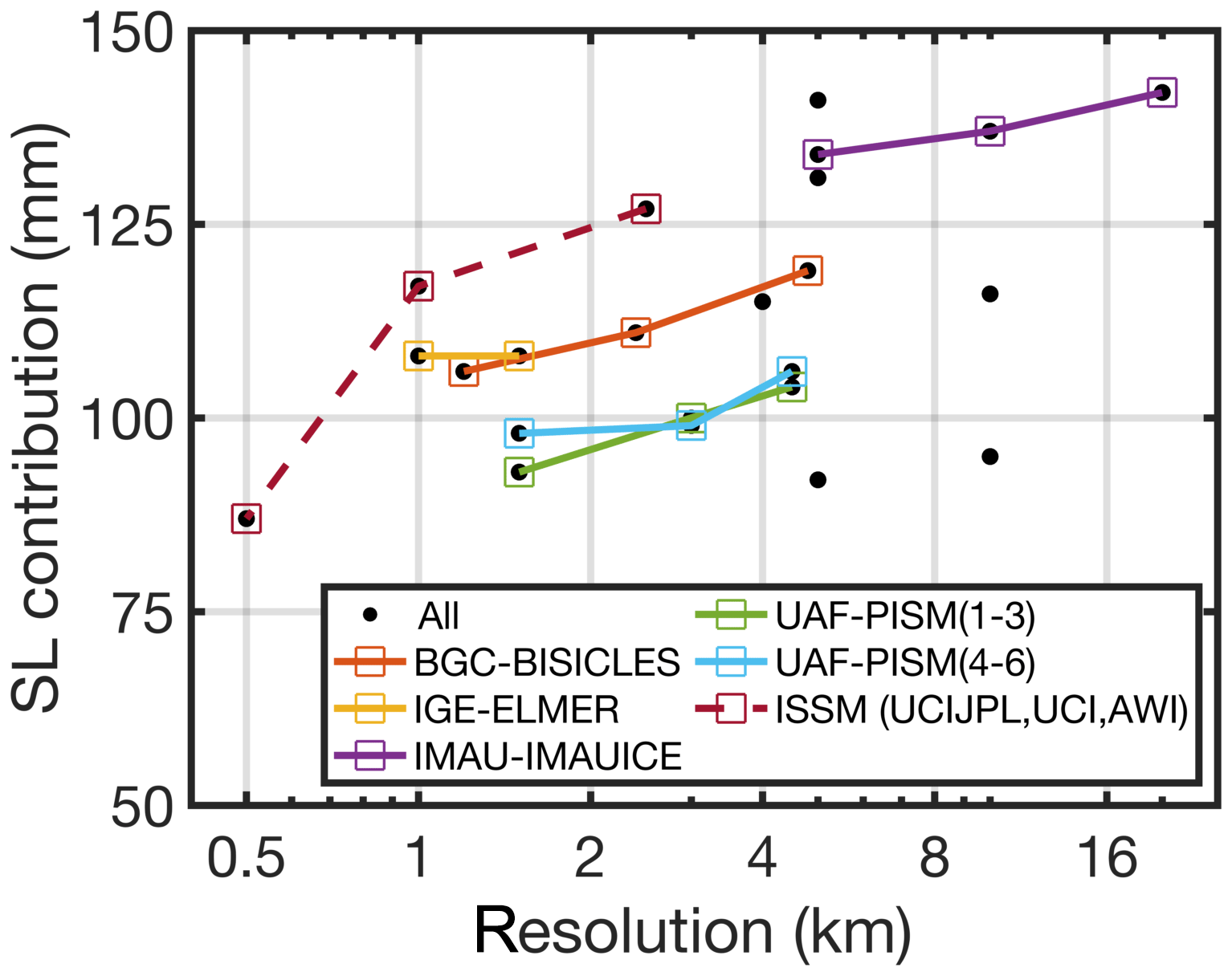
Figure 1 Results from the initMIP-Greenland exercise (Goelzer et al., 2018). Sea-level contribution vs. (minimum) horizontal grid resolution of each participating ISM. Equal model versions but different grid resolutions are connected with a coloured line. ISSM model versions are connected with a coloured dashed line. Note the logarithmic scale of the x axis. For unstructured meshes the finest resolution is displayed.

However, increasing the spatial resolution comes with the ability to resolve the geometry and to track outlet glacier behaviour (Greve and Herzfeld, 2013; Aschwanden et al., 2016). Some previous works have focused on the dependence of future mass loss of the GrIS on grid resolution (Greve and Herzfeld, 2013; Aschwanden et al., 2019). In these studies no clear conclusion on how the resolution affects the mass loss was found. This was partly explained by the competing tendencies of SMB and ice discharge that are differently resolved by the adopted resolutions. A separation of both responses in future-projection experiments would elucidate how these two main sea-level contributors from the GrIS are affected by the horizontal resolution. Most likely coarse grids underestimate ice discharge as ice flow patterns and cross sections of outlet glacier geometries are not well captured (Greve and Herzfeld, 2013; Aschwanden et al., 2016). High-resolution models, in turn, require a larger amount of computational resource. Unfortunately, when increasing the resolution, simple approximations to the momentum balance do not provide an accurate solution (Pattyn et al., 2008). This limitation takes place particularly at the ice sheet margin and at outlet glaciers where all terms in the force balance become equally important (e.g. Pattyn and Durand, 2013). Due to the intensive computational resources needed to solve the full-Stokes equation, higher-order (HO) approximations provide a good compromise to balance model accuracy and computational costs on centennial timescales.

Determining whether increased model resolution is worth the extra computation time would be valuable to make progress in narrowing uncertainties in ice sheet projections, even if only by a few per cent. The ISMIP6-Projections-Greenland shows that models with low and high resolution are found at the upper and lower bound of sea-level contribution, though no specific analysis of the grid resolution has been performed.

The main intention of this paper is to complement the study by Goelzer et al. (2020a) by evaluating the sensitivity of the simulated GrIS response to global warming due to different horizontal grid resolutions by one single ISM. Besides running the full scenarios (i.e. both oceanic and atmospheric forcing considered), we aim to explore the grid-resolution dependence on atmospheric and ocean forcing separately. Therefore, the full scenarios are complemented with experiments where either a changing SMB or the interaction of the glacier with the ocean is omitted. The simulations of the GrIS are performed with the Ice-sheet and Sea-level System Model (ISSM; Larour et al., 2012) and adopted spatial resolutions ranging from medium to high (4 and 0.75 km at fast-flowing outlet glaciers, respectively). The future scenarios build on climate-forcing data from the CMIP5 global circulation model (GCM) MIROC5 under the Representative Concentration Pathway (RCP) 8.5 (Moss et al., 2010) following the ISMIP6 protocol (Nowicki et al., 2020a).

2 Methods and experiments

Before presenting the concept of this study, we aim to address the terminology used for clarity. Following the glossary in Cogley et al. (2011), ice discharge is computed as the product of ice thickness h and the depth-averaged velocity $\overline{v}$. In the following, the lower-case q (Gt a⁻¹ m²) refers to the local ice discharge at a point and the upper-case Q (Gt a⁻¹) refers to the glacier-wide quantity (analogous to other quantities such as glacier-wide calving D and local calving d). Quantities at the margin are reckoned to be in the normal direction.

2.1 Ice flow model ISSM

The model applied here is the Ice-sheet and Sea-level System Model (ISSM; Larour et al., 2012). It has been applied successfully to the GrIS in the past (Seroussi et al., 2013; Goelzer et al., 2018; Rückamp et al., 2018, 2019a) and is also used for studies of individual drainage basins of Greenland, e.g. the Northeast Greenland Ice Stream (Choi et al., 2017), Jakobshavn Isbræ (Bondzio et al., 2017) and Petermann Glacier (Rückamp et al., 2019b). ISSM is designed to use variable ice flow approximations ranging from shallow-ice approximation to full Stokes and also has the capability to perform inverse modelling to constrain unknown parameters.

Here, we make use of the Blatter–Pattyn approximation (Blatter, 1995; Pattyn, 2003) to obtain the most accurate solution even though computational time is increased compared to simpler models (e.g. Aschwanden et al., 2019). The system of equations is solved numerically with the finite-element method, and state variables are computed on each vertex of the mesh using piecewise linear finite elements. The ice rheology is treated with a regularized Glen flow law (Glen, 1955), a temperature-dependent rate factor for cold ice and a water-content-dependent rate factor for temperate ice (Lliboutry and Duval, 1985).

At the ice base, sliding is allowed everywhere and the basal drag τ_b follows a linear viscous law (Weertman, 1957; Budd et al., 1984):

$$\begin{array}{}\text{(1)}& {\mathit{\tau }}_{\mathrm{b},i}=-k^{\mathrm{2}}N{v}_{\mathrm{b},i},\end{array}$$

where v_b,i is the basal velocity vector in the horizontal plane and $i=x,y$. Although this type of friction law is often used in ice sheet modelling (Morlighem et al., 2010; Price et al., 2011; Gillet-Chaulet et al., 2012; Seroussi et al., 2013), it implies that the basal drag can increase without a bound. It was shown that inducing an upper ratio of τ_b∕N (Iken's bound) is more justified (Iken, 1981; Schoof, 2005; Gagliardini et al., 2007; Leguy et al., 2014; Joughin et al., 2019). However, we choose this type of friction law as it is commonly used in ISMs making use of inverse methods to constrain the basal friction (Morlighem et al., 2010; Larour et al., 2012; Seroussi et al., 2013; Perego et al., 2014; Gladstone et al., 2014).

The friction coefficient k² is assumed to cover bed properties such as bed roughness. The effective pressure is defined as $N={\mathit{\varrho }}_{i}gh+min(\mathrm{0},{\mathit{\varrho }}_{\mathrm{w}}g{z}_{\mathrm{b}})$, where h is the ice thickness; z_b is the glacier base; and ${\mathit{\varrho }}_i=\mathrm{910}\mathrm{kg}{\mathrm{m}}^{-\mathrm{3}}$ and ${\mathit{\varrho }}_w=\mathrm{1028}\mathrm{kg}{\mathrm{m}}^{-\mathrm{3}}$ are the densities for ice and seawater, respectively. The parameterization accounts for full water-pressure support from the ocean wherever the ice sheet base is below sea level, even far into its interior where such a drainage system may not exist. At marine-terminating glaciers, water pressure is applied, and zero pressure is applied along land-terminating ice cliffs. A traction-free boundary condition is imposed at the ice–air interface.

The ISSM model domain for the Greenland ice sheet covers the present-day main ice sheet extent and includes the current floating ice tongues (e.g. Petermann, Ryder and 79^∘ N glaciers). The geometric input is BedMachine v3 (Morlighem et al., 2017). The thickness, bedrock and ice sheet mask is clipped to exclude glaciers and ice caps surrounding the main ice sheet. The initial ice sheet mask is manually retrieved from the data coverage of the MEaSUREs velocity data set (Joughin et al., 2016, 2018) to ensure an available target for the basal-friction inversion employed (Sect. 2.3). A minimum ice thickness of 1 m is applied. Grounding-line evolution is treated with a subgrid parameterization scheme, which tracks the grounding-line position within the element (Seroussi et al., 2014). A subgrid parameterization on partially floating elements for basal melt is applied (Seroussi and Morlighem, 2018). The basal-melt rate below floating tongues is parameterized with a Beckmann–Goosse relationship (Beckmann and Goosse, 2003). In this parameterization ocean temperature and salinity are set to −1.7 ^∘C and 35 Psu, respectively. The melt factor is roughly adjusted such that melting rates correspond to literature values (e.g. Wilson et al., 2017; Rückamp et al., 2019b). However, at most locations the grounding line coincides with the calving front. Except for the floating-tongue glaciers Petermann, Ryder and 79^∘ N, the subgrid schemes at the grounding line are not applied. The treatment of the calving-front evolution depends on the experimental setup and is explained in Sect. 2.4 and 2.5.2.

Table 1 Summary of models and their mesh characteristics. Computational time is based on a projection run under MIROC5 RCP 8.5 and medium ocean forcing.

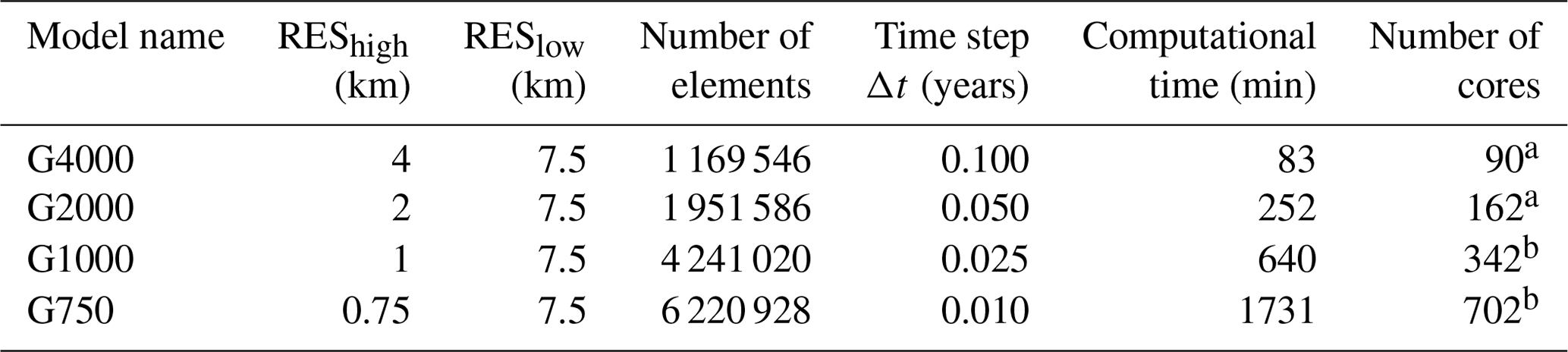
^a Intel Xeon Broadwell CPU E5-2697 v4, 2.3 GHz, on the AWI cluster system Cray CS400.
^b Intel Xeon Broadwell CPU E5-2695 v4, 2.1 GHz, on the German Climate Computing Center (DKRZ) cluster system Mistral.

As we expect the grounding line not to retreat too excessively in the projections, model calculations with ISSM are performed on a horizontally unstructured grid which remains fixed in time. To limit the number of elements while maximizing the horizontal resolution in regions where physics demands higher accuracy, the horizontal mesh is generated with a higher resolution of RES_high in fast-flowing regions (observed ice velocity > 200 m a⁻¹) and a coarser resolution of RES_low in the interior. This adaptive strategy allows a variable resolution in key areas of the ice sheet, e.g. marine-terminating outlet glaciers. Experiments are carried out at four different horizontal grid resolutions with RES_high equal to 4, 2, 1 and 0.75 km (Table 1 and Fig. 2). The distribution of mesh vertices at numerous outlet glaciers is depicted in Figs. S6 to S19 in the Supplement. In Fig. 3, the interpolated bed elevation for two selected regions and grid resolutions is illustrated. Overall, the bedrock topography of the finer resolution shows deeper and fjord-like troughs, which is closer to the BedMachine data set.

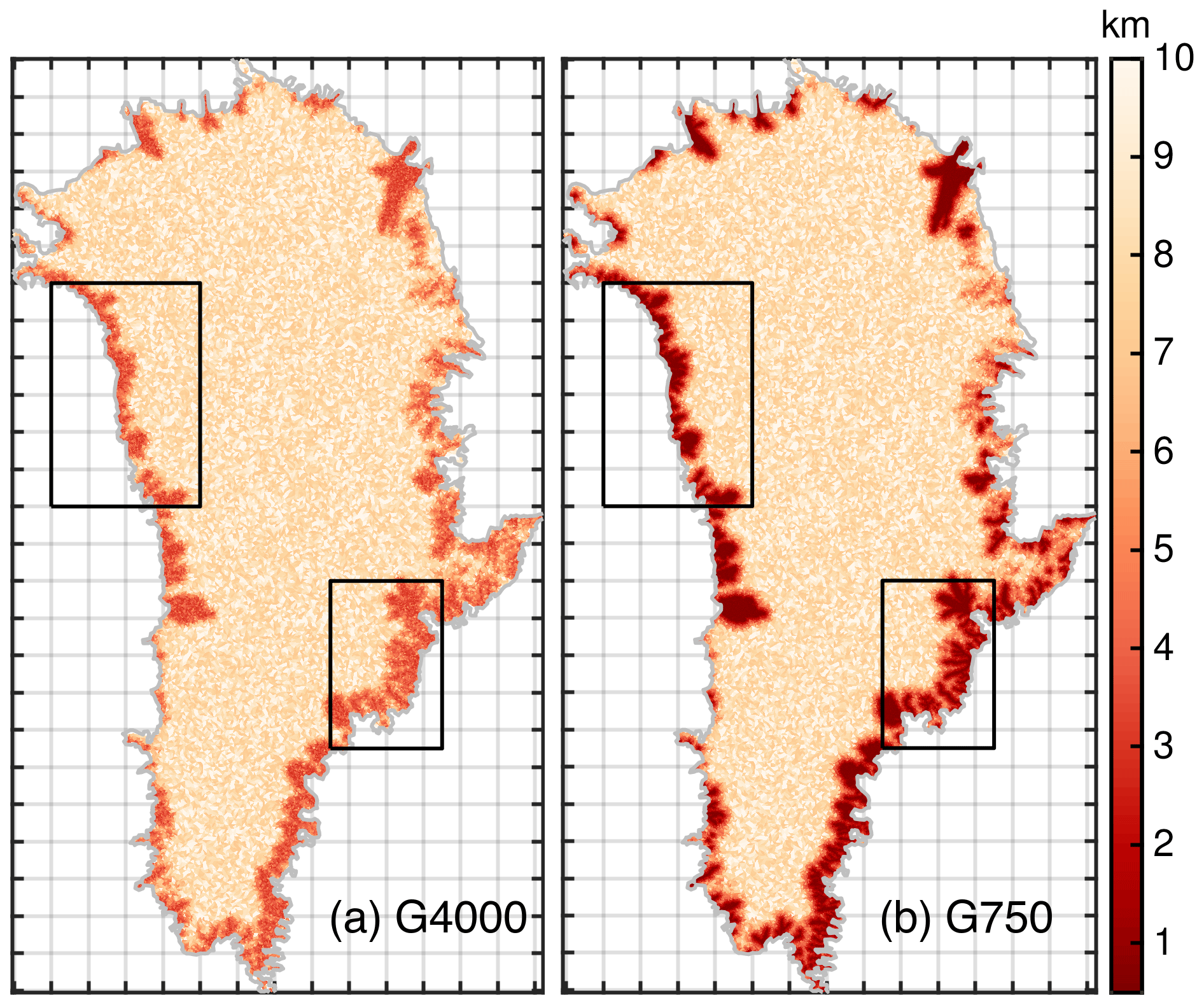
Figure 2 Horizontal mesh resolution (km) used for G4000 (a) and G750 (b). Data are clipped at 0.5 and 10 km. The horizontal resolution of a triangle is defined by its minimum edge length. The grey line delineates the initial ice domain. Grey grid lines indicate 100 km. The black boxes indicate the northwestern and southeast subsets used in following figures.

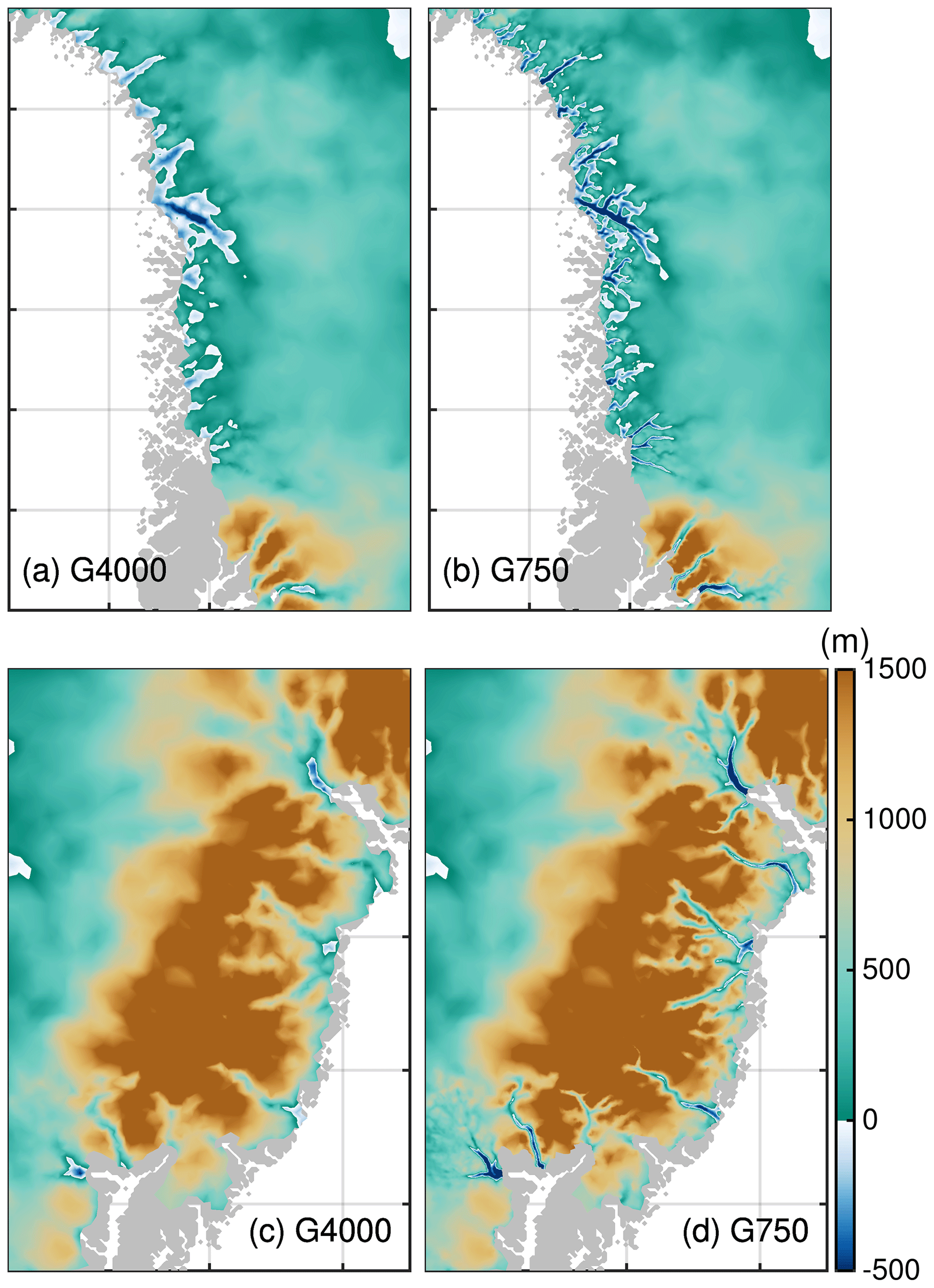
Figure 3 G4000 and G750 bedrock topography for the northwestern region (a, b, respectively), and for the southeast region (c, d, respectively). Region subsets are shown in Fig. 2.

Independent of the horizontal resolution, the vertical discretization comprises 15 terrain-following layers, refined towards the base where vertical shearing becomes more important. Please note that G1000 and G750 correspond to the ISMIP6 contributions AWI-ISSM2 and AWI-ISSM3, respectively, in Goelzer et al. (2020a).

2.2 Overview of experiments

The ISMIP6 protocol requests the initialization mode prior to or on the ISMIP6 projection start date. If the initialization date is before the start of the projections, a short historical run is needed to advance the ISM from the reference date to the end of 2014. From this date, the future-climate scenarios branch off. Unforced constant-climate control experiments are defined to capture the model drift with respect to the ISM reference climate and the ISMIP6 projection start date. The set of experiments are described in the following sections but can be summarized as follows:

• Initialization. Experiment to retrieve the initial state of the model is performed.

• ctrl. Experiment where the climate is held constant to the reference climate (from January 1991 to end of December 2100) is performed.

• ctrl_proj. Experiment where the climate is held constant to the reference climate (from January 2015 to end of December 2100) is performed.

• Historical. Experiment to bring model from the initialization state to the ISMIP6 projection start date (from January 1991 to end of December 2014) is performed.

• Projection. Future-climate scenario (from January 2015 to end of December 2100) is projected.

2.3 Initialization experiment

The initialization state of ISSM is based on data assimilation and inversion for determining the basal-friction coefficient. Before the inversion, a relaxation run assuming no sliding and a constant ice temperature of −10 ^∘C is performed to avoid spurious noise that arises from errors and biases in the data sets. To ensure that the relaxed geometry does not deviate too much from the observed geometry, the relaxation is conducted over 1 year. However, while inverse modelling is well established for estimating basal properties, the temperature field is difficult to constrain without performing an interglacial thermal spin-up. Therefore, we rely on a temperature field that was obtained by a hybrid approach between palaeoclimatic thermal spin-up and basal-friction inversion. This method was developed for the AWI contribution in initMIP-Greenland (Goelzer et al., 2018) and further improved in Rückamp et al. (2018) by using the geothermal flux pattern from Greve (2005, scenario hf pmod2). Here, we initialize the ice rheology on the four employed G4000–G750 grids by interpolating the 3-D temperature and water content fields from the hybrid spin-up in Rückamp et al. (2018). The basal-melting rates of grounded ice are equivalently interpolated. During all transient runs, we neglect an evolution of the thermal field. This is justified as it was shown by Seroussi et al. (2013) and Goelzer et al. (2018, see submissions AWI-ISSM1 and 2) that the temperature field and its change have a negligible effect on century timescale projections of the GrIS.

The main ingredient of the initialization is the inversion to infer the basal-friction coefficient k² in Eq. (1). This approach minimizes a cost function that measures the misfit between observed and modelled horizontal velocities (Morlighem et al., 2010). The cost function is composed of two terms which fit the velocities in fast- and slow-moving areas. A third term is a Tikhonov regularization to avoid oscillations. The parameters for weighting the three contributions to the cost function are taken from Seroussi et al. (2013). We leverage horizontal surface velocities from the MEaSUREs project (Joughin et al., 2016, 2018), as the data set with almost no gaps over the GrIS is suitable for basal-friction inversion.

The assigned reference year is 1990. This date is not in agreement with the timestamps of the BedMachine data set (reference time is 2007) and the MEaSUREs velocity data set (temporal coverage from 2014 to 2018). However, we ignore the contemporaneity requirement in the inversion approach and put more weight on starting the projections at the end of the assumed GrIS steady-state period (e.g. Ettema et al., 2009). All transient simulations start from the initial state; that means, we do not perform a subsequent relaxation run to bring the model to a steady state (see Sect. 2.6).

2.4 Historical and control experiments

In both control experiments (ctrl and ctrl_proj), the SMB and ice sheet mask remain unchanged from the reference year according to the ISMIP6 protocol. To advance the model from the reference time to the projection start date, the historical scenario is needed. During the historical period, yearly cumulative SMB is taken from the RACMO2.3p2 product (Noël et al., 2018) for the years from 1990 to 2015. For simplicity, the ice sheet extent remains unchanged from the reference year. This is a crude approach, but representing the historical mass loss accurately was not a strong priority for our experimental setup. As the ice front is not moving in these three scenarios, ice discharge Q equals calving D.

2.5 Future forcing experiments

It is beyond the scope of this paper to present the details of the ISMIP6 protocol and experimental design. Therefore, we aim to briefly outline the external-forcing approach. Further details are given in Goelzer et al. (2020a), Nowicki et al. (2020a), Fettweis et al. (2020) and Slater et al. (2019, 2020).

Table 2 Summary of projection experiments based on MIROC5 RCP 8.5 climate data.

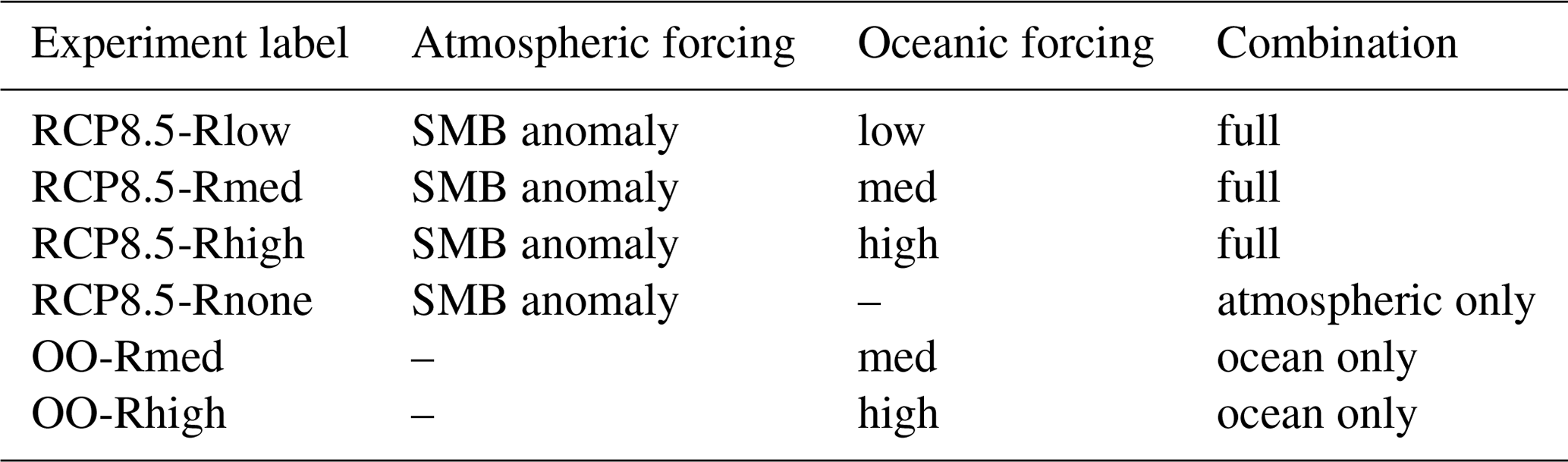
As we aim to study the effect of grid resolution on ice mass changes, we run the future scenarios based on climate data from one single GCM. The GCM MIROC5 was selected as it performs well in the historical period and represents a plausible climate near Greenland (Barthel et al., 2020). The GCM output is used to separately derive ISM forcing for the interaction with the atmosphere and the ocean. We set up experiments where both external forcings are considered; these scenarios are termed “full” in the following (RCP8.5-Rlow, RCP8.5-Rmed, RCP8.5-Rhigh). In addition, we perform simulations where either the atmospheric forcing (RCP8.5-Rnone) or the marine-terminating outlet glacier retreat (OO-Rmed, OO-Rhigh) is at play. The conducted projection experiments and the corresponding experiment labels used in this study are summarized in Table 2 and are explained in the following sections.

2.5.1 Atmospheric forcing

ISMIP6 provides surface-forcing data sets for the GrIS based on CMIP GCM simulations. The GCM output is dynamically downscaled through the higher-resolution regional climate model (RCM) MAR v3.9 (Fettweis et al., 2017). The latter allows for the capturing of narrow regions at the periphery of the Greenland ice sheet with large SMB gradients, which are likely not captured by the GCMs. The climatic SMB that is used as future-climate forcing reads

$$\begin{array}{}\text{(2)}& \begin{array}{rl}{\text{SMB}}_{\text{clim}}(x,y,t)& ={\text{SMB}}_{\text{ref}}(x,y)+\mathrm{\Delta }\text{SMB}(x,y,t)\\ & +{\text{SMB}}_{\text{dyn}}(x,y,t),\end{array}\end{array}$$

with the anomaly defined as

$$\begin{array}{}\text{(3)}& \begin{array}{rl}\mathrm{\Delta }\text{SMB}(x,y,t)& =\text{SMB}(x,y,t{)}_{\text{GCM–MAR}}\\ & -\stackrel{\mathrm{‾}}{\text{SMB}}(x,y{)}_{\text{GCM–MAR}}^{\mathrm{1960}-\mathrm{1989}},\end{array}\end{array}$$

where $\text{SMB}(x,y,t{)}_{\text{GCM–MAR}}$ is the direct output of MAR using the GCM climate data and $\stackrel{\mathrm{‾}}{\text{SMB}}(x,y{)}_{\text{GCM–MAR}}^{\mathrm{1960}-\mathrm{1989}}$ the corresponding mean value over the reference period (from January 1960 to December 1989). As the reference SMB field SMB_ref(x,y), we choose the downscaled RACMO2.3p2 product (Noël et al., 2018) whereby a model output was averaged for the period 1960–1990. This period is chosen as the ice sheet is assumed to be close to a steady state in this period. (e.g. Ettema et al., 2009). The SMB deduced by MAR is processed on a fixed topography (off-line); consequently local climate feedback processes due to the evolving surface in the projection experiments are not captured. The SMB height–elevation feedback is considered with a dynamic correction SMB_dyn to the SMB_clim following Franco et al. (2012):

$$\begin{array}{}\text{(4)}& \begin{array}{rl}{\text{SMB}}_{\text{dyn}}(x,y,t)& =\text{dSMBdz}(x,y,t)\times \left(z_s\right(x,y,t)\\ & -z_{\text{ref}}(x,y)).\end{array}\end{array}$$

The surface elevation changes are taken from the ISM elevation $z_s(x,y,t)$ while running the simulation and the corresponding ISM reference elevation z_ref(x,y) from the initialization state. The yearly patterns of $\mathrm{\Delta }\text{SMB}(x,y,t)$ and $\text{dSMBdz}(x,y,t)$ are provided by ISMIP6. A cumulative SMB anomaly over the projection period is shown in Fig. 4a.

Figure 4 Atmospheric and oceanic forcing. (a) Spatial pattern of the cumulative (2015–2100) SMB anomaly based on MIROC5 RCP 8.5 and downscaled with MAR (Fettweis et al., 2020). (b) Retreat of marine-terminating outlet glaciers in the northwestern region under RCP8.5-Rhigh scenario. Purple areas indicate retreated areas in 2100. Region subsets are shown in Fig. 2.

2.5.2 Oceanic forcing

For the oceanic forcing we rely on the empirically derived outlet glacier parameterization retreat by Slater et al. (2019, 2020). This method circumvents the problem of employing a physically based calving law and frontal-melting rates based on GCM output. When employing this parameterization to the calving front, retreat and advance of marine-terminating outlet glaciers is directly prescribed as a yearly series of ice front positions. (i.e. it is not a result of the ice velocity at the calving front, calving rate and frontal melt that are used to simulate the calving-front position). Here, the binary retreat masks (i.e. ice-covered and non-ice-covered cells) are interpolated to the native grid by nearest-neighbour interpolation. Retreat occurs once a cell is fully emptied.

Though this parameterization is a strong simplification, it builds on projected sub-marine melting taking into account changes in ocean temperature and surface meltwater runoff from a GCM. The parameterization is not applied to the individual glaciers but over a predefined geographical region. Based on the numerous retreat trajectories, a medium retreat scenario as the trajectory with the median retreat in 2100 is defined. To cover uncertainty by this approach, low- and high-retreat scenarios are defined as the trajectories with the 25th and 75th percentile retreats in 2100. In the following, these retreat scenarios are termed Rlow, Rmed and Rhigh (Table 2). The retreat mask for RCP8.5-Rhigh in 2100 is exemplarily shown in Fig. 4b. Please note that the future-projection experiment RCP8.5-Rnone experiences no retreat of marine-terminating outlet glaciers.

2.6 Comparability of experiments

Central questions about resolution dependence are always as follows: how comparable are the results, and what is controlling the results? The presented initialization procedure and involved parameters are achieved for the high-resolution simulations (G750). The simulations with a coarser resolution would probably require other parameters, e.g. to obtain a better result for observational targets or to achieve a reduced model drift. However, we decided here to keep model parameters (e.g. inversion parameters) and parameterizations (e.g. subgrid scheme at grounding line) unchanged for all simulations. Similarly to the retreat masks, we rely on binary retreat masks for all adopted resolutions although the ISMIP6 protocol requests a subgrid scheme for coarse-resolution models. On the one hand this strategy simply assumes that the results are comparable as they build on the same basis. On the other hand it avoids exploring parameter spaces which are out of the scope of this study.

For the geometric input we are following the same strategy. It is always a compromise between matching the observed geometry or being closer to a steady state. Here, we put more weight on having the initial geometry closer to the observed geometry. Therefore, we directly started the historical run after the inversion, and no further relaxation run is performed to bring the model to a steady state. As the model is likely not in a steady state at the initial state, we expect a model drift in the transient runs which would not be the case for models that perform a relaxation towards a steady state after the inversion.

3 Results

3.1 Historical scenario

To evaluate the modelling decisions pertaining to the initialization, the state of the ice sheet at the end of the historical period is compared to observations. Due to the sparseness and limited temporal and spatial coverage of available observations, we rely on the BedMachine v3 (150 m grid spacing) and MEaSUREs (250 m grid spacing) data sets for ice thickness and surface velocity, respectively. As these data are used in the data assimilation and inversion, velocity and thickness are not independent quantities. However, during the historical period the ice sheet state is altered by the boundary conditions and external forcing. Therefore, the following evaluation attempts to quantify differences from the model configurations on the ISMIP6 projection start date.

Since the results are qualitatively similar for each grid simulation (Figs. S1, S2 and S3 in the Supplement), the surface velocity field of the G750 simulation is exemplarily shown in Fig. 5a. A consequence of the employed basal-friction inversion is the high fidelity in simulating the observed-velocity field indicated by a low root mean square error (RMSE; Fig. 5b). Notable is the decreasing RMSE with increasing spatial resolution. At the end of the historical experiment the RMSE is increased compared to the initialization due to geometric and velocity adjustments over the course of the experiment. However, the ice-sheet-wide RMSE of each model version is very similar, but in the areas of fast-flowing outlet glaciers (observed velocity > 200 m a⁻¹) differences are more evident: the G4000 and G750 simulations yield $\text{RMSE}=\mathrm{150}\mathrm{m}{\mathrm{a}}^{-\mathrm{1}}$ and $\text{RMSE}=\mathrm{80}\mathrm{m}{\mathrm{a}}^{-\mathrm{1}}$, respectively. Note that these values are not identical to those given in Goelzer et al. (2020a), as the evaluation here is based on a different subsampling method. A mean signed difference (MSD) reflects a stronger underestimation of the simulated velocities with coarser resolution. The underestimation of prominent outlet glaciers for the G4000 setup is demonstrated in the spatial pattern of velocity differences (Fig. S4 in the Supplement). With increasing resolution, the difference pattern becomes more heterogeneous. Although barely visible, the G750 setup provides an interesting signature at narrowly confined outlet glaciers: generally, the velocities in the main trunk are underestimated, while beneath the shear margin velocities are overestimated. This might be due to the fact, that the employed resolution is not able to resolve the sharp velocity jump across the shear margin.

Figure 5 Simulation results and error estimate of model output at the end of the historical run compared to observations. (a) Simulated surface velocity of the GrIS (m a⁻¹) from the G750 simulation. The grey silhouette shows the Greenland land mask from BedMachine v3. Thin black lines show the grounding line. (b) Root mean square error (RMSE) of the horizontal velocity magnitude compared to MEaSUREs. (c) RMSE of ice thickness (not corrected with ctrl) compared to BedMachine v3. In panels (b) and (c), light and dark colours represent diagnostics at the initialization and end of the historical experiment, respectively. The diagnostics have been calculated on the regular MEaSUREs and BedMachine grids, respectively.

A similar evaluation for the thickness is performed. The ice-sheet-wide RMSE of ice thickness depicts the qualitatively similar grid-dependent behaviour as the velocity evaluation (Fig. 5c). Similarly, the RMSE shows larger differences in the fast-flow regions: the G4000 and G750 simulations yield RMSE=126 m and RMSE=45 m, respectively. In this region, the MSD indicates underestimation of ice thicknesses with coarser resolution. Spatial patterns of the thickness differences over the course of the historical experiment are shown in Fig. S5 in the Supplement.

The stored volumes, ice extent and spatially integrated SMB are among all grid simulations rather similar ($V=\mathrm{7.28}\mathrm{m}\mathrm{SLE}\pm \mathrm{0.2}\mathit{\%}$, A = 1.787 × 10⁶ km² ± 0.7 %, SMB = 375 Gt a⁻¹ ± 0.2 %). However, the underestimation of velocities and ice thicknesses in the coarser-resolution models is confirmed by the temporal mean of the ice discharge in the historical period. The intrinsically simulated ice discharge Q yields 207 to 341 Gt a⁻¹ for the G4000 and G750 simulations, respectively.

3.2 Sea-level contribution

In the following the transient effect of spatial resolution on ice volume evolution for the future-climate experiments is studied. The change in ice mass loss is expressed as sea-level contributions. Therefore, the simulated volume above flotation is converted into the total amount of global sea-level equivalent by assuming a constant ocean area of 3.618 × 10⁸ km². In the following, the mass losses in the projection experiments are corrected with the ctrl run with respect to the reference time. For all conducted projection experiments, the determined GrIS mass losses as a function of time are shown in Fig. 6 and listed in Table 3.

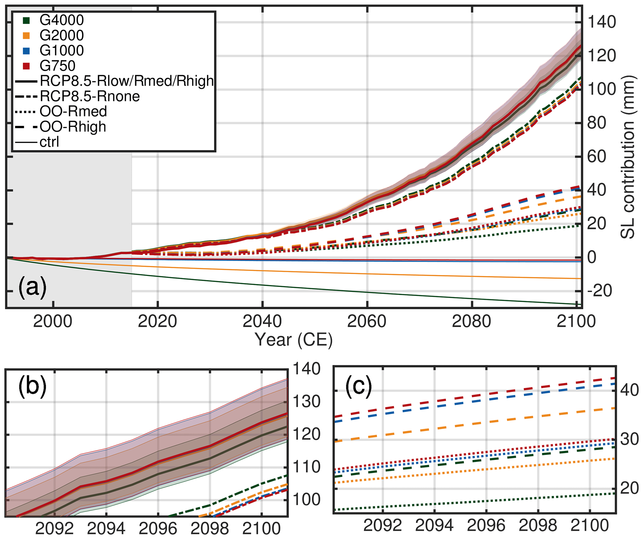
Figure 6 Projected sea-level contribution of the Greenland ice sheet based on MIROC5 RCP 8.5 climate data (a). Coloured lines indicate the different grid resolutions employed, while the individual scenarios are indicated with different line styles. The mass loss trends are corrected with the ctrl run relative to the reference time. The grey-shaded box shows the historical period. (b) Enlargement of the RCP8.5-Rlow, RCP8.5-Rmed, RCP8.5-Rhigh and RCP8.5-Rnone scenarios. (c) Enlargement of the OO-Rmed and OO-Rhigh scenarios.

Table 3 Modelled mass change (mm SLE) in future experiments for all experiments.

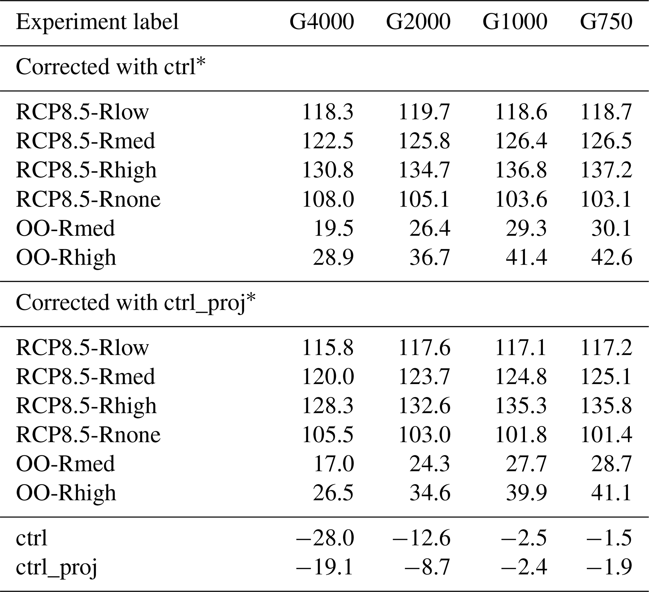
^∗ Numbers for G1000 and G750 are different compared to Goelzer et al. (2020a) as they are differently calculated (e.g. considered ocean area, native vs. interpolated
grid resolution).

As we have not initialized our model to be at a steady state, the transient response in the ctrl experiment (thin coloured lines in Fig. 6) should not be interpreted as a prediction of actual future behaviour; the ctrl run rather confirms that each model has achieved a high degree of equilibration, which is reflected by a low rate of volume change. As the initialization states are presumably different across the employed grids, we expect a different response of the ice sheet as it is likely not in equilibrium with the applied SMB and ice flux divergence. The simulated ice mass evolution shows for all models a mass gain for the 111-year ctrl experiment ranging between −28 and −2 mm. With increasing resolution, the drift gets smaller and is minimal for the G1000 and G750 simulations. Although projections are corrected with the ctrl run, the higher drift needs caution when interpreting the results as it has, e.g. a consequence on the SMB height–elevation feedback. The higher mass gain rates of the coarser resolutions in the ctrl simulation are due to the lower ice discharge rates (Sect. 3.1). Although the integrated signal in ice mass change is generally small, the spatial patterns reveal an ice thickness imbalance of up to hundreds of metres over the ctrl period (Fig. 7). Imposing an SMB correction to suppress the thickness imbalance would be feasible for maintaining a small drift. However, this is avoided here to enable a clean comparison between the four model versions and to leave the ice dynamics some degree of freedom. Moreover, the mass trends represent an important diagnostic. Comparing the ice thickness changes reveal distinct differences between the grid-resolution simulations (Fig. 7). For example, at the end of the ctrl run at some western and northwestern locations at the margin, the G4000 simulation exhibits thickening while the G750 reveals thinning. Another example is simulated at the southwestern margin, where extensive thickening prevails in all simulations but reaches farther inland in the coarser resolutions. However, from these figures, it becomes clear that positive and negative thickness changes partially compensate for each other, resulting in a low model drift.

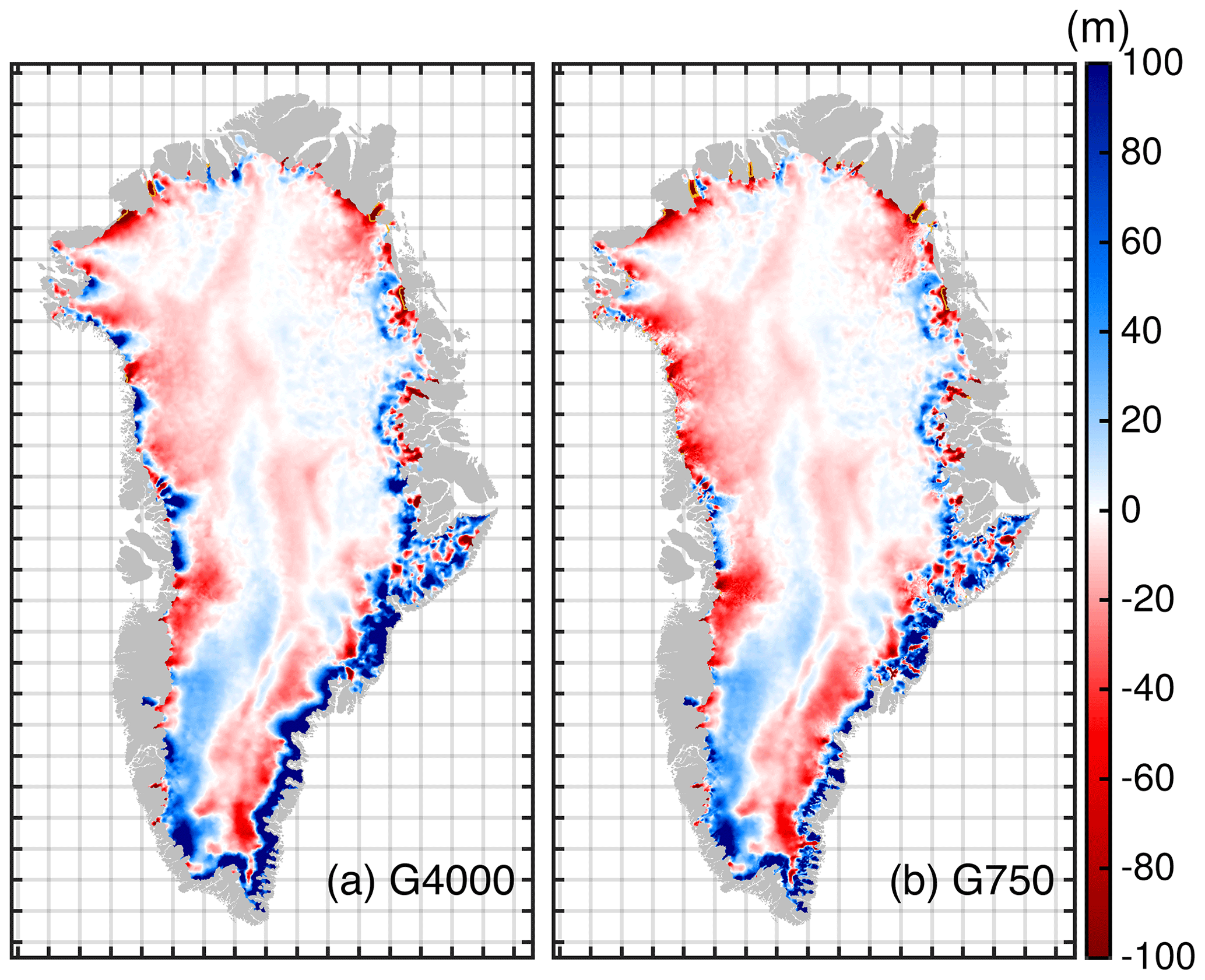
Figure 7 Difference in ice thickness between 2100 and 2015 for the ctrl run. (a) G4000 simulation and (b) G750 simulation. The grey silhouette shows the Greenland land mask from BedMachine v3. Positive values represent thickening, and negative values show thinning. Thin yellow line shows the grounding line in the year 2100.

Depending on the projection scenario, the GrIS will lose ice corresponding to an SLE of between 19 mm (or 108 mm excluding OO-Rmed and OO-Rhigh) and 137 mm. For the future-climate scenarios including atmospheric forcing a gradual increase in mass loss until the end of this century is simulated, indicating accelerating mass loss for a high-emission scenario. For RCP8.5-Rmed the mass loss reaches about 125.3 mm in 2100 (mean over G4000, G2000, G1000 and G750 results). The uncertainty quantification in the oceanic forcing results in a mean sea-level contribution that is 7.1 % less and 5.4 % greater for the RCP8.5-Rlow and RCP8.5-Rhigh scenarios, respectively. When no calving-front retreat is at play, i.e. the RCP8.5-Rnone scenario, the projected mean mass loss is approx. 105.0 mm, i.e ∼ 20 mm less compared to RCP8.5-Rmed. In contrast, the mean mass loss is considerably reduced to 26 and 37 mm in the OO-Rmed and OO-Rhigh experiment, respectively. Interestingly, a linear superposition of RCP8.5-Rnone and OO-Rmed leads to an overestimated mass loss of about 4.1 % for G4000 and 5.3 % for G750 compared to RCP8.5-Rmed where both external forcings are simultaneously at play; a linear superposition of RCP8.5-Rnone and OO-Rhigh leads to 4.5 % and 5.8 % overestimation. This is in line with earlier studies where this effect was already reported (Goelzer et al., 2013; Fürst et al., 2015)

Among all future projections a resolution-dependent impact on sea-level contribution is generally small compared to the total signal for our grids. In 2100, the spread in sea-level contribution is 6.4 mm in RCP8.5-Rhigh, 4.1 mm in RCP8.5-Rmed, 1.5 mm in RCP8.5-Rlow and 5 mm in RCP8.5-Rnone. Merely the OO-Rlow and OO-Rmed scenarios exhibit a spread of 10.7 mm and 13.6 mm, respectively, which is on the order of the absolute magnitude. A notable feature for all conducted simulations is that the sea-level contribution in each individual experiment converges with increasing resolution.

Figure 8 summarizes the qualitative behaviour of each experiment as a function of grid resolution. Note that the sea-level contribution in each experiment is normalized by its maximum. The finer resolutions tend to produce more mass loss in 2100 for the RCP8.5-Rmed, RCP8.5-Rhigh, OO-Rmed and OO-Rhigh experiments. An inverse behaviour is determined for the RCP8.5-Rnone experiment. The trend in the RCP8.5-Rlow experiment is not clear. The RCP8.5-Rnone, OO-Rmed and OO-Rhigh experiments unveil a linear behaviour as a function of grid size with regression slopes of $m=\mathrm{1.50}\mathrm{mm}{\mathrm{km}}^{-\mathrm{1}}$, $m=-\mathrm{3.27}\mathrm{mm}{\mathrm{km}}^{-\mathrm{1}}$ and $m=-\mathrm{4.18}\mathrm{mm}{\mathrm{km}}^{-\mathrm{1}}$, respectively. The trend in the full RCP8.5-Rlow, RCP8.5-Rmed and RCP8.5-Rhigh scenarios is not consistent: RCP8.5-Rmed and RCP8.5-Rhigh show a peak in mass loss at the finest resolution, whereas a peak in mass loss is attained in the G2000 simulation for RCP8.5-Rlow. For the latter, it is worth mentioning that the variations across the different grid simulations are less than 1.2 %. However, an intriguing effect of the conducted simulations remains the opposite behaviour of the RCP8.5-Rnone and e.g. RCP8.5-Rhigh scenarios. In the following section, we study this effect by analysing the mass partition to obtain a more in-depth insight into the role of atmospheric and oceanic forcing on grid resolution. It is worth mentioning that the qualitative behaviour of the detected grid-dependent mass loss remains similar when the projections are corrected with the ctrl_proj experiment (Table 3).

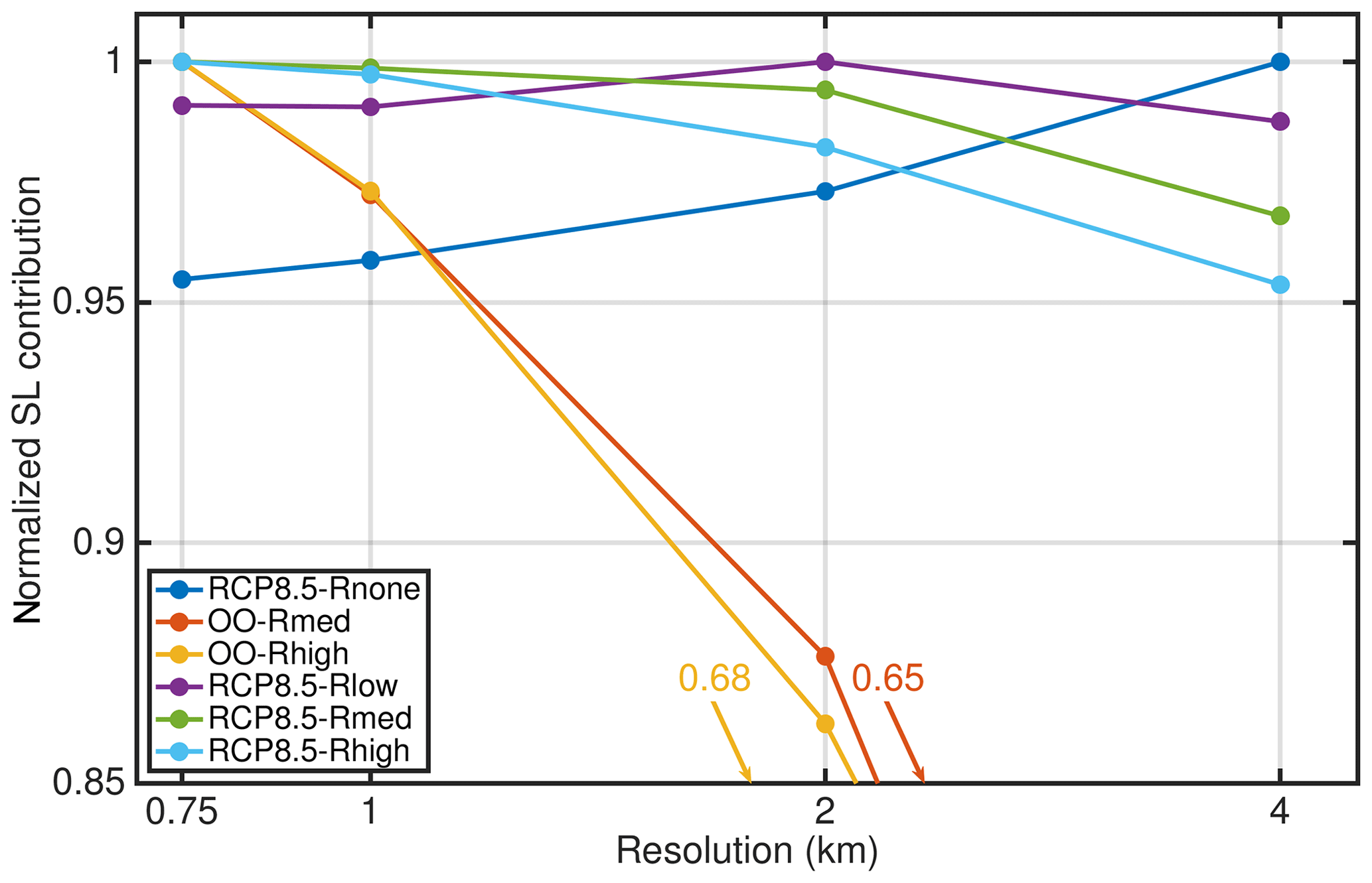
Figure 8 Projected sea-level contribution in 2100 of the Greenland ice sheet as a function of the horizontal grid size. Values are normalized to the maximum of each experiment (coloured lines). Note the logarithmic scale of the x axis.

3.3 Mass partitioning

The relative mass loss partitioning in 2100 is shown in Fig. 9 to explore the role of the grid resolution in each experiment. The bars indicate the relative importance to sea-level contribution of ice dynamic changes in the projections. The dynamic contribution (composition of front retreat and ice discharge) is calculated as the residual of the total mass change and the integrated SMB anomaly. The remainder explains the part of SMB. The overall picture reveals that for experiments that include the atmospheric forcing the SMB anomaly is the governing forcing regardless of the grid resolutions. However, the importance of the dynamic contribution increases with larger prescribed retreat rates of outlet glaciers; i.e. G750 with RCP8.5-Rhigh on the upper end shows the highest importance of dynamic contribution with up to ∼ 28.4 %. On the lower end, the RCP8.5-Rnone shows diminished importance of dynamic contribution (< 5 %). In the OO-Rmed and OO-Rhigh scenarios, the mass loss is dominated by dynamic contribution. Concerning the grid resolution, the importance is on an equal level and exceeds 100 %. The negative importance of SMB stems from the fact that the glacier retreat is cutting off regions at the ice sheet margin where the static SMB is low.

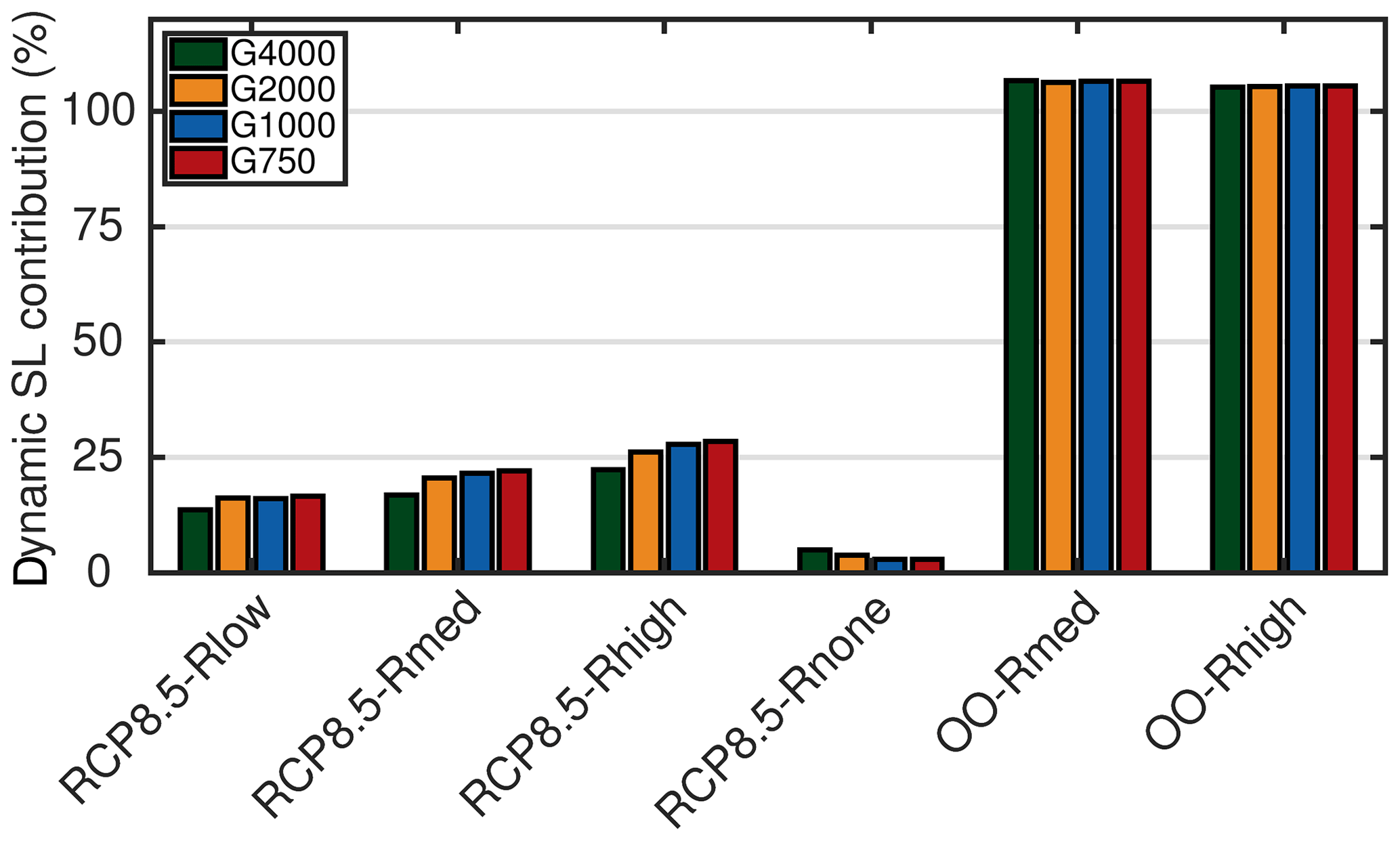
Figure 9 Mass loss partitioning for the conducted experiments. The bars indicate the relative dynamic contribution to sea level, calculated as the residual of the total of the mass change and the integrated SMB anomaly. The residual is a composition of front retreat and ice discharge.

In the full experiments RCP8.5-Rlow, RCP8.5-Rmed and RCP8.5-Rhigh, an increase in resolution enhances the importance of the dynamic contribution. For the G750 simulation it is ∼ 3 %, 5 % and 6 % higher for RCP8.5-Rlow, RCP8.5-Rmed and RCP8.5-Rhigh, respectively, compared to G4000. Curiously, the opposite behaviour is observed for the RCP8.5-Rnone experiment, where a finer resolution damps the importance of the dynamic contribution; G4000 yields a 4.9 % dynamic contribution, whereas G750 yields a 2.9 % dynamic contribution.

The simulated inverse grid-resolution responses raise the question of the driving causes. Overall the time series of the SMB show a decline and only minor differences among the grid resolutions (Fig. 10a). At the end of the projection, the cumulative SMB is 2.1 % and 2.6 % lower in the G4000 simulation for RCP8.5-Rnone and RCP8.5-Rhigh, respectively, compared to G750. These differences could be explained by different evolution of ablation areas at the margin and the SMB height–elevation feedback, in particular affected by the ctrl run, among all grid-resolution setups. In contrast, the cumulative ice discharge for these settings reveals an opposing response in the RCP8.5-Rnone and RCP8.5-Rhigh scenarios and more relative differences between the grid resolutions (Fig. 10b and c). At least for G2000, G1000 and G750, the ice discharge in the RCP8.5-Rnone experiment decreases over the century; the decrease in G4000 is offset by a few decades and exhibits an increase early in the century. These reductions explain the grid dependence of the dynamic contribution as listed in the previous paragraph (RCP8.5-Rnone in Fig. 9). For RCP8.5-Rhigh, the ice discharge shows an increase consistently but is more enhanced in the finer resolutions. This finding corroborates the grid-dependent increase in the relative ice discharge importance (RCP8.5-Rhigh in Fig. 9). As the opposing differences in RCP8.5-Rnone and RCP8.5-Rhigh are prevailing in ice discharge, it can be concluded that resolving ice discharge on the different grids is a decisive factor here. The involved feedback are further explored by focusing on particular outlet glaciers in the next section.

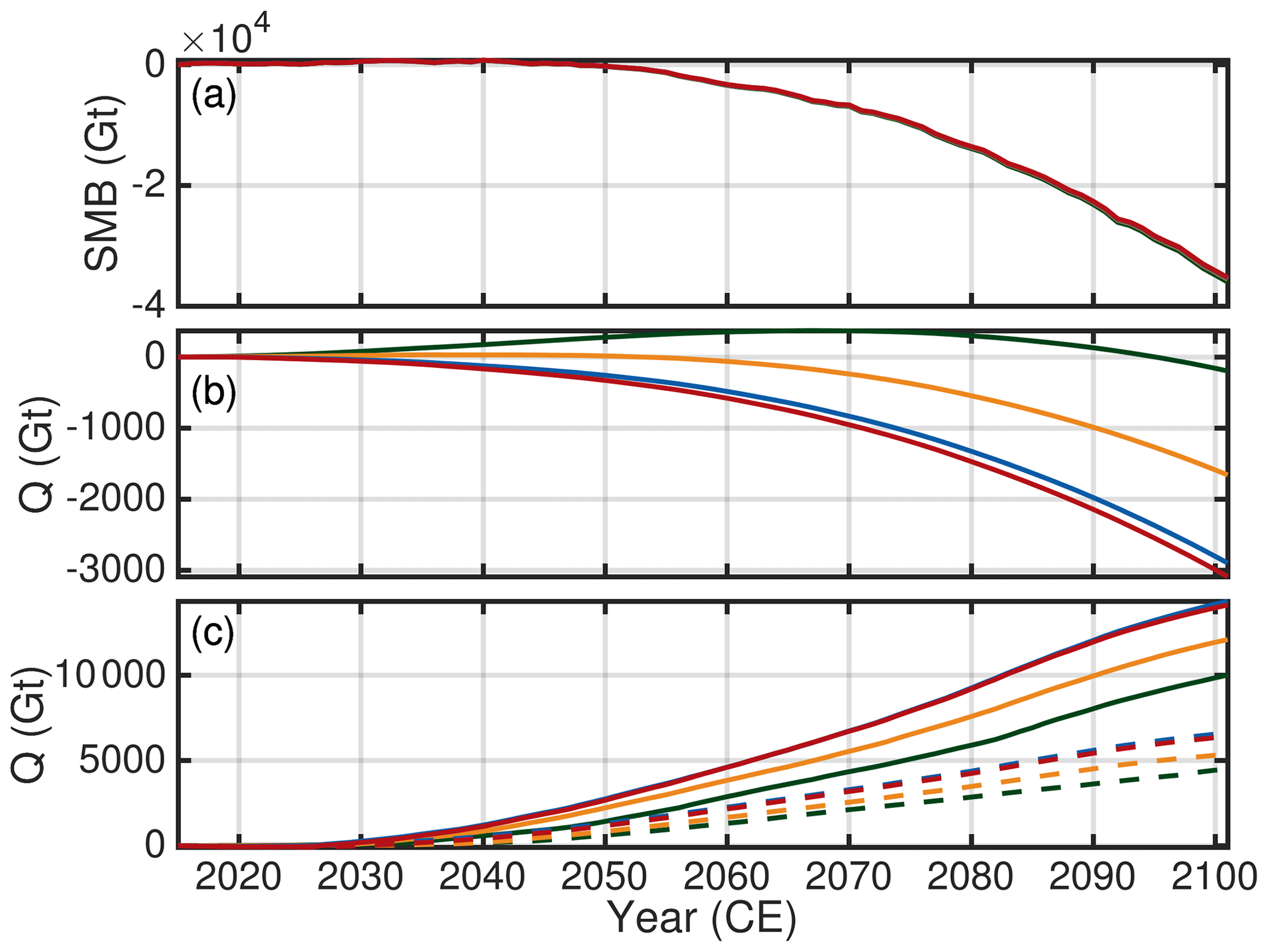
Figure 10 Time series of cumulative SMB anomaly and cumulative ice discharge Q. Colour scheme is as in previous figures. (a) Cumulative SMB anomaly for RCP8.5-Rnone. (b) Cumulative ice discharge Q for RCP8.5-Rnone. (c) Ice discharge for RCP8.5-Rhigh (solid lines) and RCP8.5-Rlow (dashed lines). Cumulative SMB anomaly for RCP8.5-Rhigh and RCP8.5-Rlow is qualitatively similar to RCP8.5-Rnone. Ice discharge is not corrected with the ctrl run.

3.4 Outlet glacier response

The fact that the centennial mass loss for the full experiments increases as the grid size reduces raises the question whether this is caused by ice dynamics alone, dominant feedback with surface mass balance or retreat, or other non-obvious factors. We conduct an in-depth analysis of numerous prominent outlet glaciers at the GrIS (Fig. S6 and table with analysis provided as separate SI). The responses of most of the outlet glaciers reveal the deduced grid-dependent behaviour where higher resolutions cause an enhanced discharge. This is exemplarily illustrated in Fig. 11a for Helheim Glacier. However, this behaviour is not visible at all selected outlet glaciers. The presented example demonstrates that the bedrock topography deviates significantly among the different grid resolutions. Generally, the bedrock topography of the coarser resolution is located above the bed of the finer resolution. This topographic effect is restricted to narrow confined outlet glaciers that obey a characteristic width on the order of a few kilometres. Outlet glaciers that have a larger characteristic width, such as Humboldt Glacier, reveal in our setups a comparable bedrock topography. These glaciers seem to have a qualitatively equal behaviour for glacier speed-up and change in ice discharge for all employed grid resolutions (Fig. 11b). This analysis demonstrates that adjacent glaciers that experience similar environmental conditions may behave differently because ice discharge is strongly controlled by glacier geometry.

Figure 11 Response of outlet glaciers. Colour scheme is the same as in previous figures, and light to dark colours indicate the years 2015, 2070 and 2100. (a) Helheim Glacier under RCP8.5-Rhigh forcing. (b) Humboldt Glacier under RCP8.5-Rhigh forcing. (c) Store Glacier under RCP8.5-Rhigh forcing. (d) Store Glacier under RCP8.5-Rnone forcing. Upper rows show the transient behaviour of the ice discharge q, the middle rows the surface velocity v and lower rows the evolution of the ice geometry. In the lower rows, the grey-shaded area depicts the bedrock topography from the G750 simulation. The grey lines from dark to light indicate the bedrock topography from the G1000, G2000 and G4000 simulation. None of the quantities are corrected with the ctrl run. Distance is relative to an arbitrary point.

Glaciers that are converted from a marine-terminating to a land-terminating glacier by retreating out of the water form their own class. These glaciers are no longer subject to the retreat and show a collapse in ice discharge regardless of the grid resolution as illustrated for Store Glacier in Fig. 11c. The qualitative behaviour of the retreat seems to be similar as reported in Aschwanden et al. (2019, Fig. 4b therein), but the timing of the retreat is different. In our study, Store Glacier is unstable and retreats within this century out of the water, while in Aschwanden et al. (2019) Store Glacier is in a very stable position; the quick retreat sets in far beyond 2100 once the glacier loses contact with the bedrock high. This different response is related to the retreat parameterization employed that lacks information on the bedrock topography, such as topographic highs and lows.

RCP8.5-Rnone shows a distinct slowdown in ice velocities as illustrated in Fig. 11d for Store Glacier. Visible is a larger slowdown of the higher resolutions; the same behaviour holds for the ice discharge q. This is in line with the finding above, i.e. that the scenario RCP8.5-Rnone reveals reduced ice discharge (Fig. 10b).

4 Discussion

The simulations presented here show that the projected sea-level contribution is sensitive to the spatial resolution. The sensitivity effect depends on the climate forcing, with oceanic and atmospheric forcings showing opposite and non-trivial responses. The simulations have shown that the ice discharge to the ocean is a decisive factor here controlling the grid-dependent spread. As shown above, outlet glaciers respond differently to external forcing, depending on the employed grids and geometrical setting. In such a non-linear system examining a driving mechanism remains challenging. However, despite the somewhat heterogeneous response of outlet glaciers, the different scenarios tend to produce an overall trend in characteristic fields that explains the different responses.

The different responses in the full scenarios could be attributed to the ability to resolve bedrock topography and the interaction with basal sliding. Figure 12 illustrates spatial changes in the effective pressure and basal-sliding velocity for RCP8.5-Rhigh. A common characteristic for G750 is a stronger decrease in effective pressure, which is concentrated in areas where the finer grid shows a deeper bed of the marine portions compared to G4000. Due to the linear dependence of τ_b on effective pressure (Eq. 1), basal-sliding velocities increase more strongly in the finer resolution. This feedback is enhanced as the SMB perturbations lead to a decrease in ice thickness, hence to a decrease in the effective pressure. The transient evolution reveals further that thinning and acceleration propagate faster and farther upstream in the finer resolution. The higher signal propagation rates may have additional consequences on longer timescales as the surface melt is amplified by the positive surface mass balance–elevation feedback exposing the ice surface to higher air temperatures.

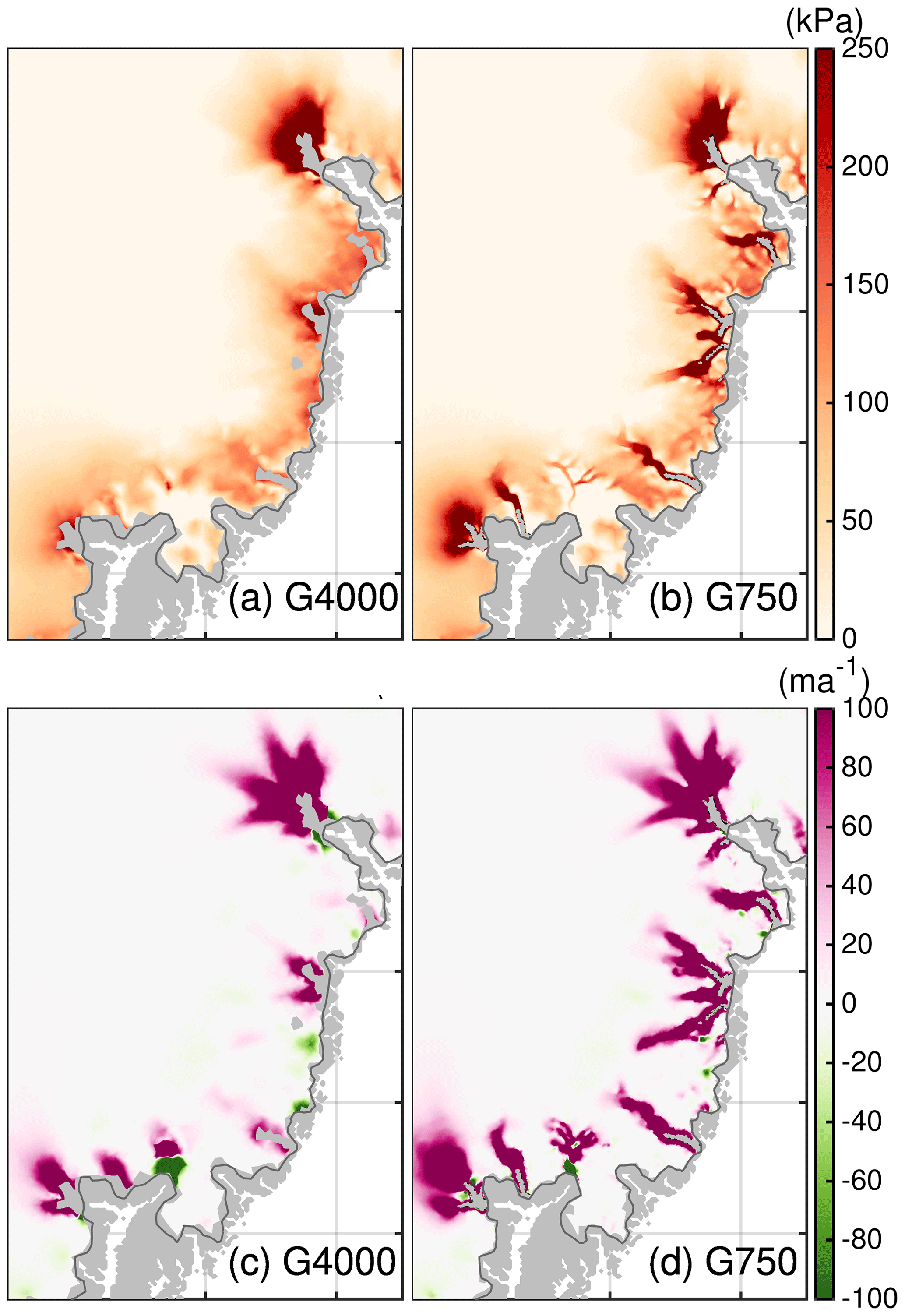
Figure 12 (a, b) Difference in effective pressure between 2100 and 2015 for the southeast region. (c, d) Difference in basal velocity between 2100 and 2015 for the southeast region. Region subsets are shown in Fig. 2. Dark grey line indicates the initial ice extent. Thin black line indicating the grounding line is not visible as it falls together with the calving front. The grey silhouette shows the Greenland land mask from BedMachine v3.

It remains questionable if the widespread glacier acceleration is induced by the frontal stress perturbation instead of the decrease in the effective pressure. To isolate this effect we conduct a RCP8.5-Rhigh simulation (not shown) where the effective pressure is held constant to the historical level. This setup reveals a very limited acceleration of a few glaciers in the G4000 simulation; some show no response or even a slowdown. In the corresponding G750 simulation most of the outlet glaciers show a speed-up, but this effect is very localized and does not reach far upstream. Therefore, we conclude, that the pronounced decrease in the effective pressure along with the acceleration of outlet glaciers is a dominant mechanism controlling the grid-dependent spread.

In order to investigate whether the response behaviour is an effect of purely reducing the grid size, we repeated the OO-Rhigh and RCP8.5-Rhigh experiments with a G1000 simulation using regridded bedrock topography and a friction coefficient from the G4000 initial state (simulations are not shown). This setup adopts a high-resolution grid but omits detailed information from the high-resolution input data. Projected mass loss by this setup is closer to the G4000 simulation. It, therefore, demonstrates that a high model resolution alone is insufficient to explain the grid-dependent sea-level contribution. As a consequence, a driving cause of the grid-dependent behaviour arises from additional information in the input data. Therefore, we conclude that the grid-dependent behaviour is highly connected to the bedrock topography because the different models represent the bedrock topography quite differently.

Compared to the full and ocean-only scenario, the atmospheric-only scenario unveils a stronger mass loss for the coarse resolution. To some extent, this could be explained by a slightly lower SMB in the coarser resolution. However, the finer resolution produces a stronger reduction in ice discharge over the course of the experiment. Although for many of the outlet glaciers the effective pressure decreases (not as strongly as for the scenarios with considered retreat), there is instead a slowdown of most glaciers (Fig. 13c and d). Again, these differences are concentrated in areas where the finer grid shows deeper troughs. Curiously, the finer resolution is better able to resolve these details, but the velocity evolution causes an extra reduction in ice discharge compared to in the coarser resolution. This non-trivial response is illustrated with the change in driving stress, approximated as ${\mathit{\tau }}_{\mathrm{d}}={\mathit{\varrho }}_{i}gh\left|\text{grad}{z}_s\right|$ (Fig. 13a and b). Compared to 2015, the driving stress has locally decreased more in the finer resolution in 2100 compared to the coarser resolution; away from the marginal region, the driving-stress changes are on a comparable magnitude for all employed grids. These results indicate that the reduction in the effective pressure is outperformed by geometric adjustments in the RCP8.5-Rnone scenario. This experiment intended to omit an interaction of the glacier with a changing ocean forcing, but the assumption of a fixed calving front hinders outlet glaciers from adjusting freely to topographic changes. They, therefore, do not experience reduced buttressing or frontal stress perturbations which are necessary mechanisms to trigger widespread glacier acceleration (e.g. Bondzio et al., 2017). In future studies, it might be desirable to allow the calving front to adjust although the oceanic forcing is held constant. Nevertheless, the simulations indicate that without a frontal stress perturbation an ensuing speed-up of the outlet glacier is not initiated. This highlights the importance of capturing calving events, i.e tracking the ice front position in numerical models, most accurately.

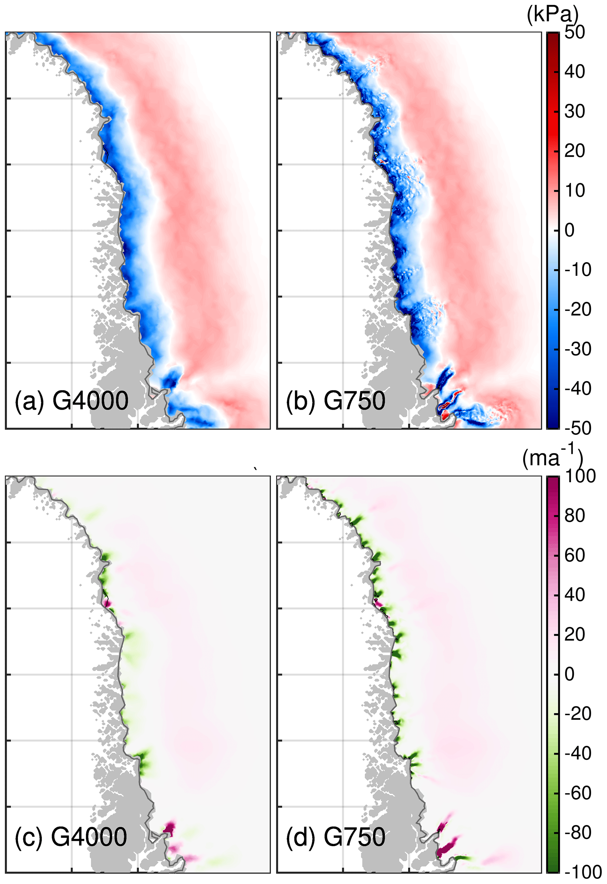
Figure 13 (a, b) Difference in driving stress between 2100 and 2015 for the northwestern region. (c, d) Difference in basal velocity between 2100 and 2015 for the northwestern region. Region subsets are shown in Fig. 2. Dark grey line indicates the initial ice extent. Thin black line indicating the grounding line is not visible as it falls together with the calving front. The grey silhouette shows the Greenland land mask from BedMachine v3.

The inverse grid-dependent behaviour of the RCP8.5-Rnone, OO-Rmed and OO-Rhigh scenarios has some implications when interpreting the mass loss of the ice sheet. The combined scenarios demonstrate that in a particular case, the sea-level contribution is maximized for an intermediate resolution. Depending on the horizontal grid resolution, the competing tendencies of SMB and ice discharge are differently resolved. This finding seems to corroborate results by Aschwanden et al. (2019), where an intermediate resolution reveals the largest sea-level contribution.

A convergence of the grid-dependent estimates of sea-level contribution emerges around RES_high≤ 1 km. This value corroborates Aschwanden et al. (2016) for capturing outlet glacier behaviour indicating an upper limit for horizontal grid resolution. However, the converging behaviour should be treated with some caution. We cannot exclude the possibility that a model resolution finer than 750 m would lead to results that deviate from the convergence. On the one hand, the 150 m horizontal grid spacing of the BedMachine v3 data set is much finer than our finest resolution of 750 m. As the retreat parameterization is insensitive to bed undulations, resolving the outlet glacier cross sections is important for accurately modelling ice discharge. Since the glacier cross sections are reasonably well approximated in G750, we do not expect that resolving the geometry in a higher resolution would drastically alter ice discharge rates. On the other hand, there are indications that at a resolution of 750 m the HO solution is not fully converged (Pattyn et al., 2008). Adopting a higher resolution could have implications for the ice flow and hence for the evolution of ice discharge. Likewise, in Aschwanden et al. (2019, Fig. S4 therein), the ice discharge is shown to increase as the mesh resolution is increased and seems to converge below a resolution of ≤ 1800 m. However, the finer resolutions of 450 and 600 m seem to produce again a somewhat lower ice discharge. This might indicate that the underlying processes are not fully converged and still causing changes in mass loss trends.

Our grid-dependent results under atmospheric-only forcing correlate with the finding in Goelzer et al. (2018, Fig. 1) and Exp. C2 in Greve and Herzfeld (2013, Fig. 7a and b therein). Interestingly, the causes for the same behaviour seem to have different origins. In Goelzer et al. (2018) the effect is likely due to an overestimated ablation area (see also Goelzer et al., 2020b), whereas in our study the effect is attributed to the change in ice discharge of the ice sheet. The cause for the grid-dependent behaviour in Greve and Herzfeld (2013) is not specified further. Still, it is worth mentioning that they report a much better agreement of simulated to observed surface velocities by increasing the spatial resolution. Our experiments with the considered retreat of outlet glaciers could not be compared to the S1, M2 and R8 experiments in Greve and Herzfeld (2013). On the one hand, the external-forcing approach differs. On the other hand, a grid-dependent behaviour in Greve and Herzfeld (2013) is not clear (except for the enhanced sliding experiment S1, where the finer-resolution setups show a higher response). However, please note that the comparison to Aschwanden et al. (2019) and Greve and Herzfeld (2013) is limited as the studies employ different flow approximations and treat basal friction differently. The underlying physics in each ISM probably depends differently on the resolution.

Besides the fixed calving front in the atmospheric-only scenario, further limitations of our study must be noted. The spread of projected sea-level contribution among all grids is likely subject to the chosen type of friction law. The choice of the basal-friction law used in ISMs remains a matter of debate (Stearns and van der Veen, 2018; Minchew et al., 2019) and a potential source of uncertainty in sea-level projections (e.g. Brondex et al., 2019). Compared to our used type of friction law, there are some indications that friction laws satisfying an upper bound for the basal drag are more reliable (e.g. Schoof, 2005; Gagliardini et al., 2007; Leguy et al., 2014; Joughin et al., 2019). In brief, these types of friction laws invoke a switch for the friction regimes (low and high N, respectively) so that the influence of the effective pressure on the basal drag at slow ice flow is vanishing. It would be most interesting to evaluate their sensitivity to the horizontal resolution for projections on centennial timescales.

Another limitation concerns the choice of inversion parameters. We performed the inversions for basal parameters for each grid resolution individually but relying on the inversion parameters tuned for the high-resolution setups. Effectively, this results in an overall comparable pattern for the flow velocities (Figs. S1 and S2) and basal-friction coefficient (Fig. S3) for all grids. However, on smaller scales, the inversion approach produces significantly different k² in many glacier basins. Recalling the relationship between N and k², these different patterns are plausible but could potentially be a result from non-optimal inversion parameters. However, these different spatial patterns might make an additional contribution to the grid dependence of the simulations. In future studies, it will be worth investigating this influence only, e.g. by tuning the inversion parameters for each grid separately to find the optimal parameters.

However, the simulations conducted here reveal a grid-dependent spread in the full scenarios ranging between 1.2 % and 5.3 %, which is of a comparable magnitude to the surface mass balance–elevation feedback (Eq. 4). The latter is recognized as an important mechanism and accounts for an additional sea-level contribution of about 6 %–8 % (Goelzer et al., 2020a). A feedback that we have not considered is the enhanced surface melt influencing the basal conditions and calving by filling up crevasses. Given that we greatly simplify the representation of N, the effect of a reorganization of basal conditions (in either way) or the effect of increased availability of water due to increasing surface melt on basal sliding is suppressed. To overcome this limitation, an adequate subglacial hydrology model could be invoked, even if not considering seasonality. A subglacial hydrology model has shown the localized effect on N, which likely has consequences for the spread between the employed grid resolutions (e.g. Werder et al., 2013; de Fleurian et al., 2016; Rathmann et al., 2017; Sommers et al., 2018; Beyer et al., 2018; Neckel et al., 2020).

A feedback that is not fully covered in our simulations is shear margin weakening and its influence on the evolution of flow velocities. Although the shear margins are weakly developed in the simulations (more pronounced in the finer resolutions), it is expected that a thermo-mechanical coupling could further weaken the shear margins as a response to frontal stress perturbations (e.g. Bondzio et al., 2017). Such a coupling would increase the widespread inland flow acceleration and enhance the rate of mass loss. However, the change in τ_b and τ_d is very pronounced in and around the main trunks and quite different for the adopted grids (see Figs. S20 and S21 in the Supplement). These patterns exemplify the need for resolving the shear margins in a particularly high resolution, which we have not fully accomplished in this study as shear margins are becoming, in numerous cases, subgrid phenomena. This may be a reason for under-representing glacier velocities inside the main trunk and overestimating velocities outside the main flow as apparent in G750. This effect shall be addressed in further studies, in which ideally higher resolutions are employed or error estimators are engaged (e.g. dos Santos et al., 2019).

5 Conclusions

We applied the three-dimensional finite-element higher-order model ISSM to the Greenland ice sheet to simulate the future response under climatic changes specified by the ISMIP6 protocol. The sensitivity of mass changes to the spatial resolution is tested by employing four different grids with a varying horizontal resolution ranging from 4 to 0.75 km at fast-flowing outlet glaciers. The simulations reveal up to ∼ 5.3 % more sea-level rise compared to the coarser resolution in the full scenario RCP8.5-Rhigh and ∼ 3.2 % for RCP8.5-Rmed. In scenarios where a change in SMB is omitted and only outlet glacier retreat is at play, the finer resolutions produce significantly more mass loss (up to 33 %). When no retreat is enforced, the sensitivity of the grid dependence exhibits an inverse behaviour; i.e. the coarser resolutions produce more mass loss. This finding is important to recognize for ice sheet models that have SMB as the dominant mass loss driver.

The results presented underline the importance of resolving the bedrock topography accurately. Areas with simple and low bedrock undulations experience a similar response in all model resolutions. In areas with complex and high bedrock undulations striking differences between the employed grids emerge. A mechanism that exerts an important control on the resolution-dependent spread is basal sliding predominantly in marine portions of outlet glaciers. Since we rely on a greatly simplified effective-pressure parameterization, further work is needed to prove the robustness of this conclusion.

Given the strong interaction of the bedrock topography with sliding, it is obvious that the major outlet glacier should be surveyed with the latest radar technology to obtain a substantially improved survey of the bedrock topography, the area of expected retreat and connected areas further upstream. This, in turn, requires ice sheet models ready to resolve these areas in terms of grids and physics adequately.