the Creative Commons Attribution 4.0 License.
the Creative Commons Attribution 4.0 License.
 | 02 Oct 2020
Monitoring the seasonal changes of an englacial conduit network using repeated ground-penetrating radar measurements
Melchior Grab
Cédric Schmelzbach
Andreas Bauder
Hansruedi Maurer
Englacial conduits act as water pathways to feed surface meltwater into the subglacial drainage system. A change of meltwater into the subglacial drainage system can alter the glacier's dynamics. Between 2012 and 2019, repeated 25 MHz ground-penetrating radar (GPR) surveys were carried out over an active englacial conduit network within the ablation area of the temperate Rhonegletscher, Switzerland. In 2012, 2016, and 2017 GPR measurements were carried out only once a year, and an englacial conduit was detected in 2017. In 2018 and 2019 the repetition survey rate was increased to monitor seasonal variations in the detected englacial conduit. The resulting GPR data were processed using an impedance inversion workflow to compute GPR reflection coefficients and layer impedances, which are indicative of the conduit's infill material. The spatial and temporal evolution of the reflection coefficients also provided insights into the morphology of the Rhonegletscher's englacial conduit network. During the summer melt seasons, we observed an active, water-filled, sediment-transporting englacial conduit network that yielded large negative GPR reflection coefficients (). The GPR surveys conducted during the summer provided evidence that the englacial conduit was 15–20 m±6 m wide, thick, long with a shallow inclination (2∘), and having a sinusoidal shape from the GPR data. We speculate that extensional hydraulic fracturing is responsible for the formation of the conduit as a result of the conduit network geometry observed and from borehole observations. Synthetic GPR waveform modelling using a thin water-filled conduit showed that a conduit thickness larger than 0.4 m (0.3× minimum wavelength) thick can be correctly identified using 25 MHz GPR data. During the winter periods, the englacial conduit no longer transports water and either physically closed or became very thin (<0.1 m), thereby producing small negative reflection coefficients that are caused by either sediments lying within the closed conduit or water within the very thin conduit. Furthermore, the englacial conduit reactivated during the following melt season at an identical position as in the previous year.
- Article
(32541 KB) - Full-text XML
-
Supplement
(4529 KB) - BibTeX
- EndNote


Surface meltwater is routed through the glacier's interior by englacial drainage systems, before it reaches subglacial drainage systems (Fountain and Walder, 1998; Cuffey and Paterson, 2010). Subglacial drainage systems play an important role in the dynamics of glaciers (Iken et al., 1996; Bingham et al., 2008). For example, water flowing along the base of a glacier can facilitate glacial sliding by lubricating the ice–bed interface (Hewitt, 2013). With an increase in subglacial water pressure, the ice–bed friction weakens, resulting in a faster sliding velocity (Iken and Bindschadler, 1986; Zwally et al., 2002). The subglacial water pressure can dramatically increase, if either the englacial or subglacial drainage systems do not adapt quickly to an increased meltwater input. Furthermore, the water pressure can increase depending on how water is routed through the glacier's drainage system. There is often a short time lag, in the region of hours and days, between the start of surface melting and an increase in glacier velocity (Bingham et al., 2005). Englacial drainage systems often provide the meltwater pathways that can facilitate changes in subglacial water pressure, and as a result they can impact the glacier's dynamics. Furthermore, knowledge of the englacial conduit's seasonal evolution and geometry is important for a glacier's hydrological modelling. Therefore, studying the seasonal evolution of an englacial drainage system throughout the melt season is key to understand how and when the englacial drainage system transports water into the subglacial drainage systems.
There exist different mechanisms for the formation of englacial drainage networks and these are broadly dependent on the temperature of ice. Ice below the pressure melting point (cold ice) is impermeable, and until recently (Vatne, 2001; Boon and Sharp, 2003) it was assumed that surface meltwater has limited penetration within cold-ice glaciers. However, recent research has provided evidence that englacial drainage networks are present in cold-ice glaciers and they are formed by three distinct mechanisms (Benn et al., 2009; Gulley, 2009). The first mechanism includes surface meltwater that creates incisions on the glacier's surface, and these surface streams can become englacial, if their upper levels become blocked or close due to ice creep. Such englacial streams are known as “cut-and-closure” conduits and were first described by Fountain and Walder (1998) and later by Vatne (2001) and Gulley et al. (2009a). The second mechanism for the formation of englacial conduits within cold ice is hydraulically assisted fracture propagation (Boon and Sharp, 2003; van der Veen, 2007). Englacial conduits can develop from water-filled crevasses where ice has become stressed and the water pressure within the fracture is large enough to overcome the fracture toughness of the surrounding ice. The third mechanism is related to the exploitation of permeable structures within the body of the glacier, such as fractures (Fountain et al., 2005) or debris-filled crevasses (Gulley and Benn, 2007).
The englacial drainage network theory was originally developed for ice at the pressure melting point (temperate ice) (Shreve, 1972; Röthlisberger, 1972). Temperate ice was assumed to be permeable, and this led to the theoretical model that englacial conduits form from water flowing between ice crystal boundaries within connected veins. Lliboutry (1971) argued that englacial conduits have difficulty forming within connected veins as a result of deformation and recrystallisation of the grains closing intergranular channels. Furthermore, field observations by Gulley et al. (2009b) have resulted in the formation mechanisms of englacial conduits within temperate ice being questioned. As within cold ice, englacial conduits seem to form as a result of hydraulically assisted fracture propagation in temperate ice (Gulley, 2009). Additionally, englacial conduits can form from the exploitation of pre-existing fractures (Fountain et al., 2005; Gulley et al., 2009a).
There exist only a limited number of studies investigating englacial conduit conditions on temperate ice. Studies of glacier's drainage systems are based primarily on dye tracer experiments, speleology, borehole studies, geophysical measurements, or a combination of these techniques. Englacial drainage systems have been interpreted from dye tracer testing on temperate glaciers (Nienow et al., 1996, 1998; Hock et al., 1999), but difficulties can arise in tracer testing, since they do not offer direct observations of englacial drainage networks. Direct observations have been made into inactive englacial channels using speleology techniques (Gulley, 2009; Naegeli et al., 2014; Temminghoff et al., 2019), but they were obviously conducted only when the drainage system was dry and inactive. Therefore, such observations do not provide temporal information on the englacial conduit's seasonal evolution.
Geophysical experiments can provide observations on active englacial conduit networks covering a large spatial distribution, and they can be repeated, thereby providing information on the temporal evolution. Two geophysical methods have regularly been used for studying the glacier's hydrological systems, seismology (active and passive) and radar. Ground-penetrating-radar (GPR) has been used to detect englacial drainage systems in cold ice (Moorman and Michel, 2000; Stuart, 2003; Catania et al., 2008; Catania and Neumann, 2010; Schaap et al., 2019; Hansen et al., 2020) and temperate ice (Arcone and Yankielun, 2000; Hart et al., 2015). There exist only a small number of studies that investigate seasonal changes within the englacial hydrological network, and all of these have been undertaken on cold-ice glaciers. Across several years, GPR measurements were performed by Bælum and Benn (2011) over a small cold-ice valley glacier to investigate the glacier's thermal regime. Pettersson et al. (2003) used time-lapse GPR imaging, separated by 12 years, to detect changes to the cold–temperate ice transition surface, and Irvine-Fynn et al. (2006) used repeated GPR measurements to investigate hydrological seasonal changes on a polythermal glacier. However, for these studies the GPR profiles were not repeated several times during a year and across a number of years. Therefore, very limited information is available on the seasonal evolution of englacial drainage systems, and there is little knowledge of these changes within temperate glaciers.
Reflectivity analysis is commonly employed on GPR data in order to provide subsurface properties and to identify subsurface materials. The strength of the reflected GPR signal is a function of media's electrical properties that form an interface and can therefore be used to determine subglacial environments. Such studies have been conducted with an impulse ice-penetrating radar system within a cold-ice environment (Macgregor et al., 2011; Christianson et al., 2016); however no such analysis has been performed using a commercial GPR within a temperate ice environment or to characterise an englacial conduit network. In order to extract the reflectivity from a commercial GPR system, an inversion workflow can be implemented (Schmelzbach et al., 2012). Within a glaciological environment such an inversion workflow can provide constraints on temporal and spatial changes in glacier hydrology. Temporal and spatial changes have been obtained using repeated GPR amplitude analysis and such studies have been completed in non-glaciological settings (Truss et al., 2007; Guo et al., 2014). Such investigations have not yet been conducted within a glaciological environment to detect hydrological changes.
Alongside GPR, passive seismology has been employed to identify and characterise the subglacial drainage network (Gimbert et al., 2016; Bartholomaus et al., 2015). Such an approach has recently been used to investigate subglacial conduits on temperate glaciers (Vore et al., 2019; Lindner et al., 2020; Nanni et al., 2020). Passive seismology can be a complementary tool to GPR reflectivity analysis in order to monitor seasonal evolution of the glacier's hydrological system. Our primary focus of our study is to use the GPR reflectivity analysis to detect seasonal changes within an englacial conduit network.
In this study, we use a comprehensive GPR dataset that includes GPR profiles from 2012, 2016, and 2017 and repeated GPR seasonal profiles during 2018 and 2019. GPR imaging and reflectivity analysis facilitates studying the temporal and spatial changes of an englacial conduit network on a temperate glacier. By repeating GPR measurements several times throughout the melt seasons, we can gain insights into how an englacial network changes and evolves in response to the meltwater supply. Additionally, by performing GPR measurements across subsequent melt seasons, we can verify whether these englacial networks were reactivated after the winter period in a similar location or whether they close down and become inactive the following melt season. We detect these seasonal and annual changes by extracting the GPR reflection strength (reflectivity) using a GPR impedance inversion scheme (Schmelzbach et al., 2012). The spatial extent of the reflectivity patterns allows potential englacial flow paths to be imaged. Alongside the GPR data, we were able to directly observe the englacial conduit network using a borehole camera in 2018. In brief, there are three main objectives of this research, namely
-
to implement a GPR processing routine to extract GPR reflection coefficients related to englacial structures,
-
to interpret the spatial reflection coefficients in order to gain an understanding of the temporal conduit morphology, and
-
to correlate the englacial conduit's dimensions to previous studies in order to understand the conduit's formation mechanisms.
Furthermore, we used a GPR data simulation algorithm using a variety of 3D englacial conduit models in order to quantify the spatial dimensions of an active englacial conduit network.
This englacial network monitoring case study was conducted on the Rhonegletscher (Fig. 1), where an englacial conduit network was previously detected using active seismic reflection data (Church et al., 2019). The Rhonegletscher is the sixth largest glacier in the Swiss Alps (Farinotti et al., 2009), and it is the source of the Rhône River. The glacier has been well studied and documented due to the ease of access from the nearby Furka Pass, with the first measurements from the beginning of the 17th century (Mercanton, 1916). The glacier flows southwards from 3600 down to 2200 m above sea level (a.s.l.) with a surface area of approximately 16 km2 (Huss and Farinotti, 2012). In recent years, a proglacial lake formed as a result of the glacier retreating (Tsutaki et al., 2013; Church et al., 2018). This proglacial lake is dammed by a granite riegel, and there is likely a hydraulic interaction between the lake and the glacier's drainage network. The survey site was located within the lower ablation area between 2280 and 2350 m a.s.l., where the ice thickness in 2017 was approximately 100 m (Fig. 1).
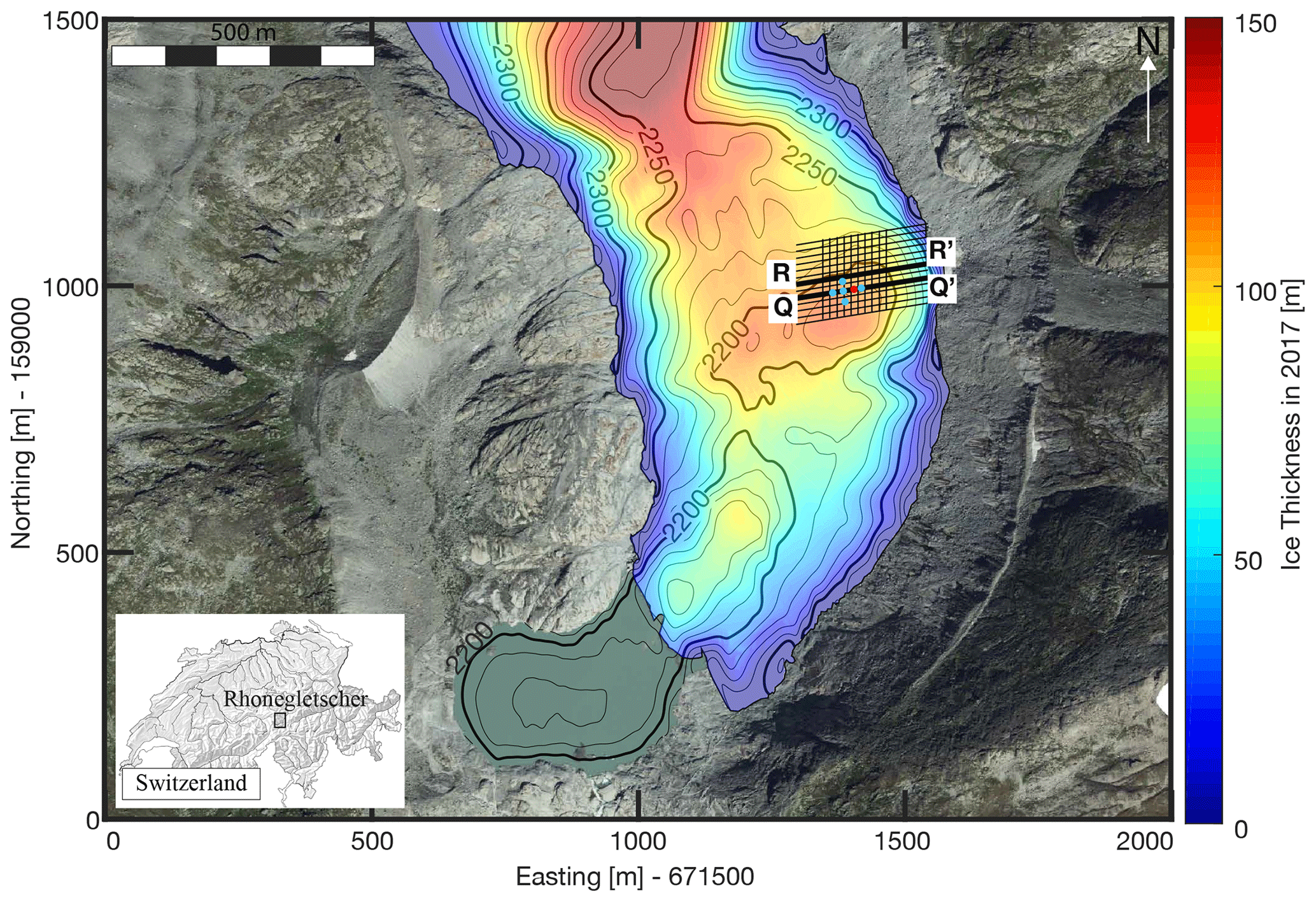
Figure 1Map of the Rhonegletscher's lower ablation area, ice thickness (colour-coding), basal topography (black contour lines) updated from Church et al. (2018), and GPR repeated survey site (black grid). The two thicker GPR profile lines (R-R′ and Q-Q′) are displayed in Figs. 3 and 4. Five boreholes were drilled in August 2018 to provide ground truths on the conduit and are marked as blue and red dots. The red dot represents the borehole where the borehole camera acquired a video.
3.1 GPR data acquisition
To investigate seasonal englacial conduit variations, we performed 13 GPR field campaigns from 2012 until 2019 (Table 1). Three GPR surveys that covered a single profile across the survey site (Q-Q′ in Fig. 1), were conducted over three different years (2012, 2016, and 2017). Upon detection of an englacial GPR reflection, which was later identified as an englacial conduit network (details on the identification of the network can be found in Church et al., 2019), we performed a dense GPR grid at different times of the year in 2018 and 2019 over the englacial conduit network (grids of black lines in Fig. 1). The GPR grid includes 13 profiles oriented east–west (average length: 250 m) and 10 profiles oriented north–south (average length: 150 m), with a spacing of 13 m between adjacent profiles.
The majority of the field measurements were conducted as common offset (CO) surveys, and they were acquired using a Sensor & Software pulseEKKO Pro GPR system with 25 MHz antennas. CO measurements are acquired keeping the transmitting and receiving antennas at a constant distance apart (known as offset), which allows large quantities of data to be collected in a time-efficient manner. The GPR antennas were carried by hand during summer month acquisitions (snow-free, June–October), and during winter month acquisitions (snow covered, November–May) they were mounted and pulled on pulk sleds. The GPR antennas were positioned in a transverse electric (TE) broadside configuration and kept at a constant offset of 4 m between transmitting and receiving antennas. Additionally, the orientation of the antennas was perpendicular to the walking direction. For all GPR lines, a high-precision global navigation satellite system (GNSS) continuously recorded the GPR antennas' midpoint, and the accuracy given by the GNSS was generally below 0.05 m.
In addition to the CO profiles, we acquired common midpoint (CMP) data in order to evaluate the electromagnetic (EM) wave velocity of the glacial ice. CMP's are acquired by incrementally increasing the offset between the transmitting and receiving antennas over a given central location such that we image a point in the subsurface with different offsets. These CMP measurements were performed in April, May, September, and October 2018 over the englacial conduit in order to detect any seasonal changes to the EM-wave velocities. The location of the CMPs was directly over the englacial conduit (marked by the green line in Fig. 2c).
3.2 Borehole data acquisition
In 2018, six boreholes were drilled around the englacial conduit network (Fig. 1) using a hot water drill. Two boreholes were drilled directly into the conduit network, and we were able to lower a borehole camera (GeoVISION™ Dual-Scan) within these boreholes to make direct observations within the englacial conduit network.
Table 1Overview of the GPR surveys acquired over the englacial conduit network. Survey months in italic and bold represent the winter (snow-covered) and summer (snow-free) acquisitions respectively, and the asterisk marks the months where common midpoint measurements were additionally acquired.

3.3 GPR data processing
The raw CO GPR data were processed using a combination of an in-house MATLAB-based toolbox (GPRglaz; Rutishauser et al., 2016; Langhammer et al., 2017; Grab et al., 2018) and Seismic Unix. The processing scheme aims to recover the GPR reflection coefficients from the englacial conduit reflections by means of an impedance inversion scheme. This inversion scheme is based upon the seismic impedance inversion developed in the late 1970s and 1980s (Russell, 1988). The reflectivity is recovered by the inversion on preconditioned GPR data using the underlying assumption that the GPR reflectivity is represented by a series of sparsely distributed spikes; this inversion is known as a sparse-spiking deconvolution (Velis, 2008). The aim of the sparse-spiking deconvolution operator is to find the smallest number of spikes that, after convolution with the GPR source wavelet, match the preconditioned GPR data within a small error. Within a glaciological setting, the spikes from the deconvolution would represent englacial reflectors or the glacier base. The workflow implemented was based upon the processing described in Schmelzbach et al. (2012).
An outline of the GPR CO processing is described in Table 2. It consists of the following major steps: (1–6) preprocessing by assigning the GNSS data with the GPR data, setting time zero and the record length, interpolating clipped data, bandpass filtering to remove noise, trace binning to account for varying walking speeds, and elevation static correction; (7) deterministic amplitude correction to compensate for the amplitude decay due to geometrical spreading, absorption, and transmission losses; (8) GPR deconvolution to remove the GPR source wavelet and increase the vertical resolution (Schmelzbach and Huber, 2015); (9) an amplitude-preserving migration to reposition the reflections in their correct location and to increase the horizontal resolution; (10) identifying an amplitude-matching scalar in order to match the amplitudes across all GPR surveys; and (11–13) sparse-spike deconvolution to recover the reflectivity (Sacchi, 1997) and to calibrate the reflectivity and stretch the reflectivity to depth below glacier surface. In order to calibrate the reflectivity, ground truth data were used. The reflectivity within the vicinity of the borehole was calibrated to be the ice–water reflectivity as direct observations provided a flowing water-filled conduit (Church et al., 2019). The outcome of this workflow after migration (9) is shown in Figs. 2 and 3a–e. The final output (13), including the reflection coefficients, is displayed in Fig. 3f–i.
Schmelzbach et al., 2012Schmelzbach and Huber (2015)Sacchi (1997)
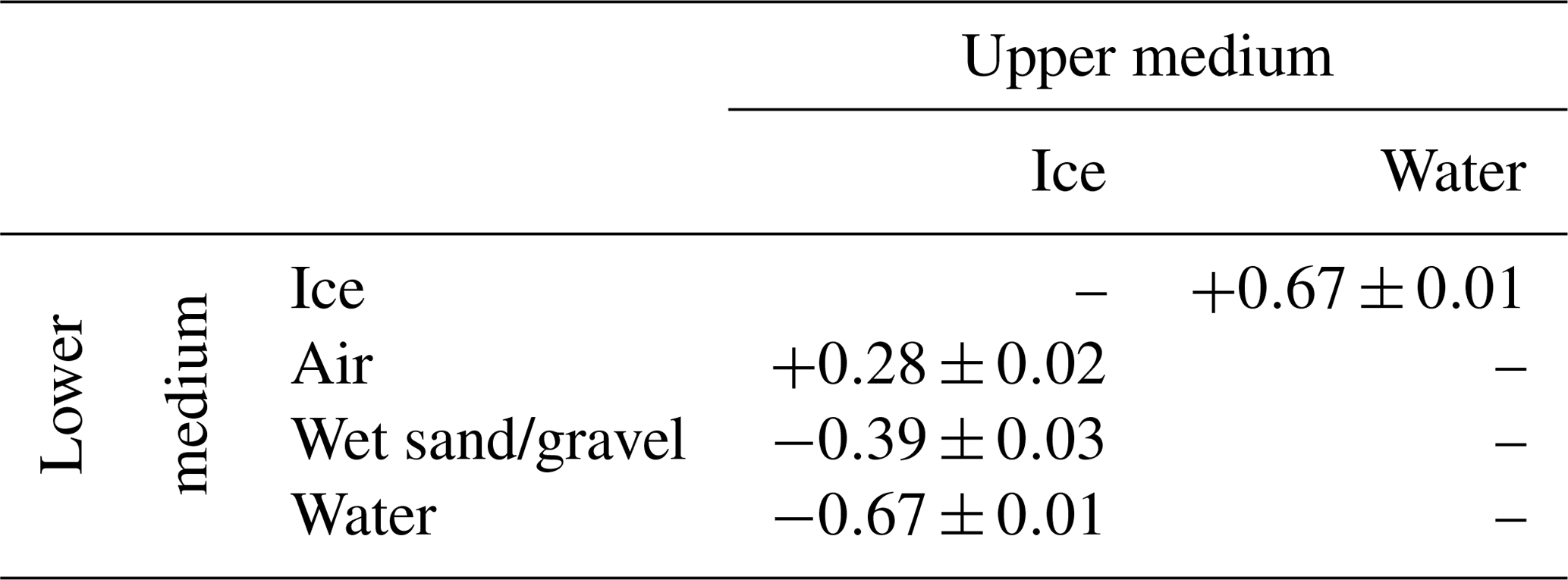
The spatial and temporal distribution of the reflection coefficients is the primary outcome of the processing workflow. The amplitude reflection coefficient explains the proportions of energy that are reflected from a given interface. Its values range between −1 and 1. Their magnitudes and polarities are indicative of the electrical material properties adjacent to an interface. For zero offset (vertical incidence), example reflection coefficients for englacial environments are provided in Table 3 using relative permittivity ranges from Reynolds (2011).
The GPR reflection coefficient has previously been used in order to determine the presence of water or bed conditions on Matanuska Glacier in Alaska, USA (Arcone et al., 1995). In the Rhonegletscher case study, we will make use of the reflection coefficient for imaging the spatial extent and the temporal evolution of the englacial conduit, and it will also provide information on the filling material within the conduit.
The GPR reflectivity workflow provides both the englacial conduit top and bottom reflection time (thickness if the filling material is known) and the englacial channel reflectivity. To provide details on seasonal evolution, both the extracted reflectivity and conduit thickness from the field data were interpolated and smoothed for each seasonal GPR acquisition.
Table 3GPR reflection coefficients from typical englacial conduit environments using zero-offset measurements.
The CMP measurements were also processed using GPRglaz, but SeisSpace ProMAX 2-D was used for the EM wave propagation velocity analysis. The preprocessing included assigning the geometry and amplitude correction for geometrical spreading. As described by Booth et al. (2010), we applied a static shift prior to picking the velocities in ProMAX in order to remove the systematic error in semblance analysis of GPR CMP data. The EM wave propagation velocities were picked on the englacial reflection using a second-order normal moveout correction; this velocity was used for the migration velocity in the workflow indicated in Table 2.
4.1 GPR imaging results
For studying the general evolution of the englacial conduit network we analysed all GPR profiles; however we consider profile Q-Q′ (location shown in Fig. 1) as an example for the annual evolution. In Fig. 2, the GPR sections acquired during the summer months are displayed. Due to the increased presence of water during the summer melt season (average daily discharge in Fig. S4), the signature of a potential englacial conduit is expected to be most pronounced during this time of the year as a result of water filling the conduit. As shown in Fig. 2a, in September 2012 there is no obvious englacial reflection spanning the section, but in September 2017, we observe a strong englacial reflection pattern at about 2210 m a.s.l. (Fig. 2b). This feature is also visible in the GPR sections acquired in summer 2018 and 2019 (Fig. 2c and d), although its shape and strengths exhibit some minor variations. From these observations we conclude that this englacial feature has undergone significant evolution between 2012 and 2017.
Besides the annual changes of this englacial feature, it is also interesting to study its seasonal variability. We analysed all GPR profiles within the grid between 2018 and 2019; however, we consider profile R-R′ (location shown in Fig. 1) as an example for the seasonal imaging results. In Fig. 3, the GPR sections, acquired in 2018 and 2019, are displayed. Additionally, the spatial distribution of the reflectivity (reflection coefficients) is provided. The single continuous englacial reflector is present across the majority of the acquired profile during the summer months (Fig. 3c and e), whereas in April 2018 (winter) it is almost absent (Fig. 3b), and its reflection strength is also reduced in May 2019 (winter) (Fig. 3d). The reflectivity (Fig. 3f–i) emphasises the contrasting englacial environment between summer and winter. Similar observations were also made in profile Q-Q′ (Fig. S2) and across the majority of GPR profiles acquired, but in profile R-R′ they are more pronounced.
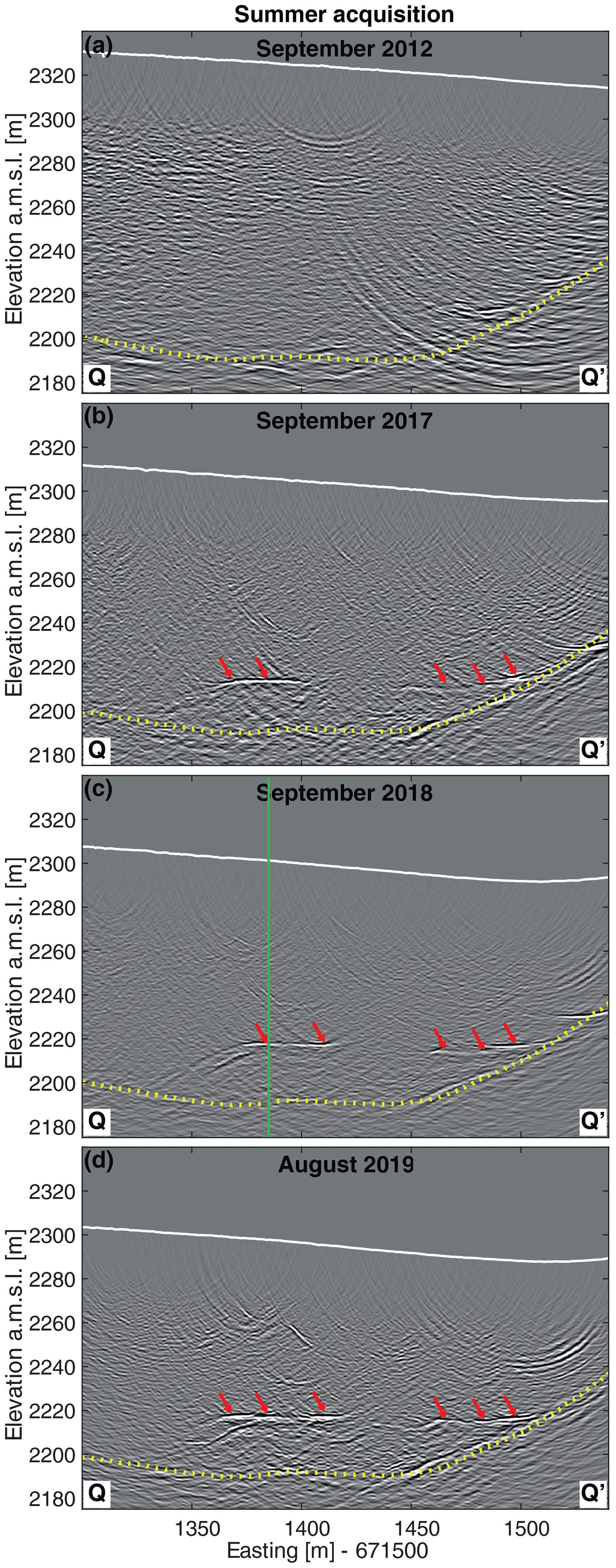
Figure 2Annual GPR imaging results from a repeated profile (Q-Q′ in Fig. 1) over a single line after migration from 2012 until 2019. The yellow line represents the ice–bedrock interface, and the red arrows represent the englacial conduit network reflection appearing from summer 2017. The green line in (c) marks the location of the CMP acquired. Zoomed GPR profile images are available in Fig. S1 in the Supplement.

Figure 3(a) Seasonal GPR imaging results over a single repeated GPR profile (R-R′ in Fig. 1) in 2018. The yellow line represents the ice–bedrock interface, the white line represents the glacier surface, and the red box is the zoom box for GPR imaging and reflectivity results (b–i). Panels (b)–(e) are seasonal GPR imaging results, and (f)–(i) are the seasonal GPR reflectivity results from (b)–(e). The red arrows represent the top of the englacial conduit network, and the blue arrows represent the bottom of the englacial conduit network (g, i).
4.2 GPR common midpoint (CMP) results
The EM wave propagation velocity for the winter CMP measurement (Fig. 4a) was picked to be 0.165±0.05 m ns−1 (Fig. 4b–c). The EM wave propagation velocity during the summer CMP measurement (October 2019) was picked at 0.170±0.05 m ns−1. There is an uncertainty in the EM wave propagation velocities as a result of limited transmitter–receiver offsets in comparison to the target depth (offset-depth ratio: 0.5), and the low-frequency antenna with a dominant period of 15 ns creates large semblance bullseyes in Fig. 4c and f. Two more CMP gathers were recorded in May and September 2019, which show a similar velocity, but with a larger uncertainty (±0.1 m ns−1) due to poorer data quality.
As a result of the uncertainties on the propagation velocities from the CMP measurements, the migration velocity was kept constant for both summer and winter at 0.1689 m ns−1 as used in previous temperate ice GPR studies (Glen and Paren, 1975; Rutishauser et al., 2016).
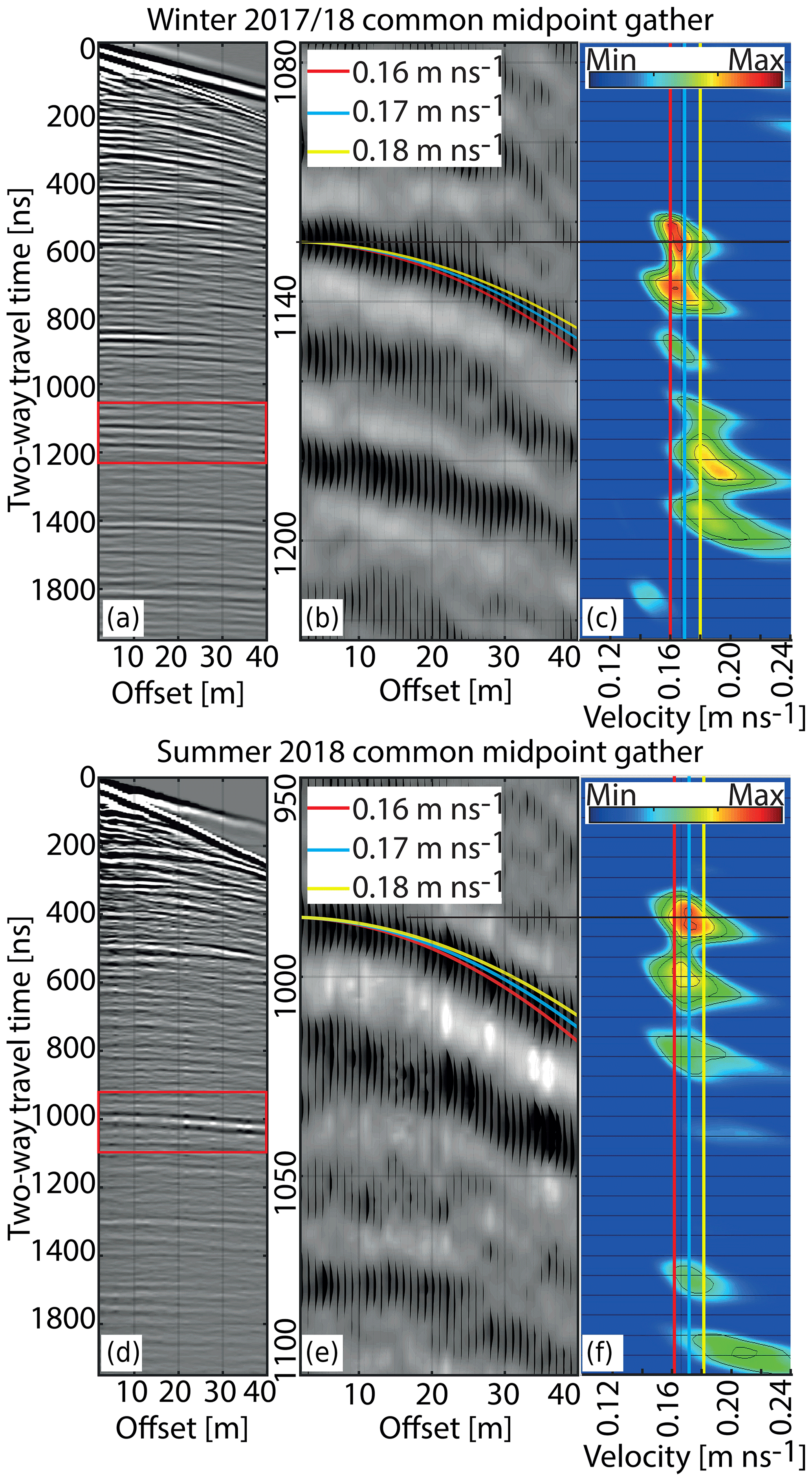
Figure 4Common midpoint gather and velocity determination. Winter (April 2018): (a) the raw CMP gather; (b) zoom of the raw gather over the englacial reflection with second-order normal moveout (NMO) curves using 0.16, 0.17, and 0.18 m ns−1. (c) Semblance display using second-order NMO for the zoom section from (b). Summer (October 2018): (d)–(f) as per winter (a–c).
4.3 GPR seasonal reflectivity results
Figure 5 highlights the seasonal spatial reflectivity over 16 months from May 2018 until August 2019. During the summer months, when the englacial conduit is active and transporting meltwater through the glacier's body, we observe large negative reflectivities (). The spatial extent of the englacial network is visible in the summer month acquisitions.
The reflectivity during the winter months (Fig. 5a–c and g–h) is around zero, indicating that there is a lack of a reflection, and the conduit is not filled with air, water, or wet sand. During the summer months (Fig. 5d–f, i) the reflectivity varies between −0.2 and −0.6, corresponding to either an ice–wet sand interface or an ice–water interface (Table 3). At the beginning of the melt season in July 2018 (Fig. 5d), the englacial conduit network does not appear to be fully connected throughout the survey site, while in September and October 2018 (Fig. 5e, f), the conduit is connected across the survey site. Furthermore, in August 2019 (Fig. 5i), we observe reflectivities between −0.2 and −0.6 in a similar location as in summer 2018.
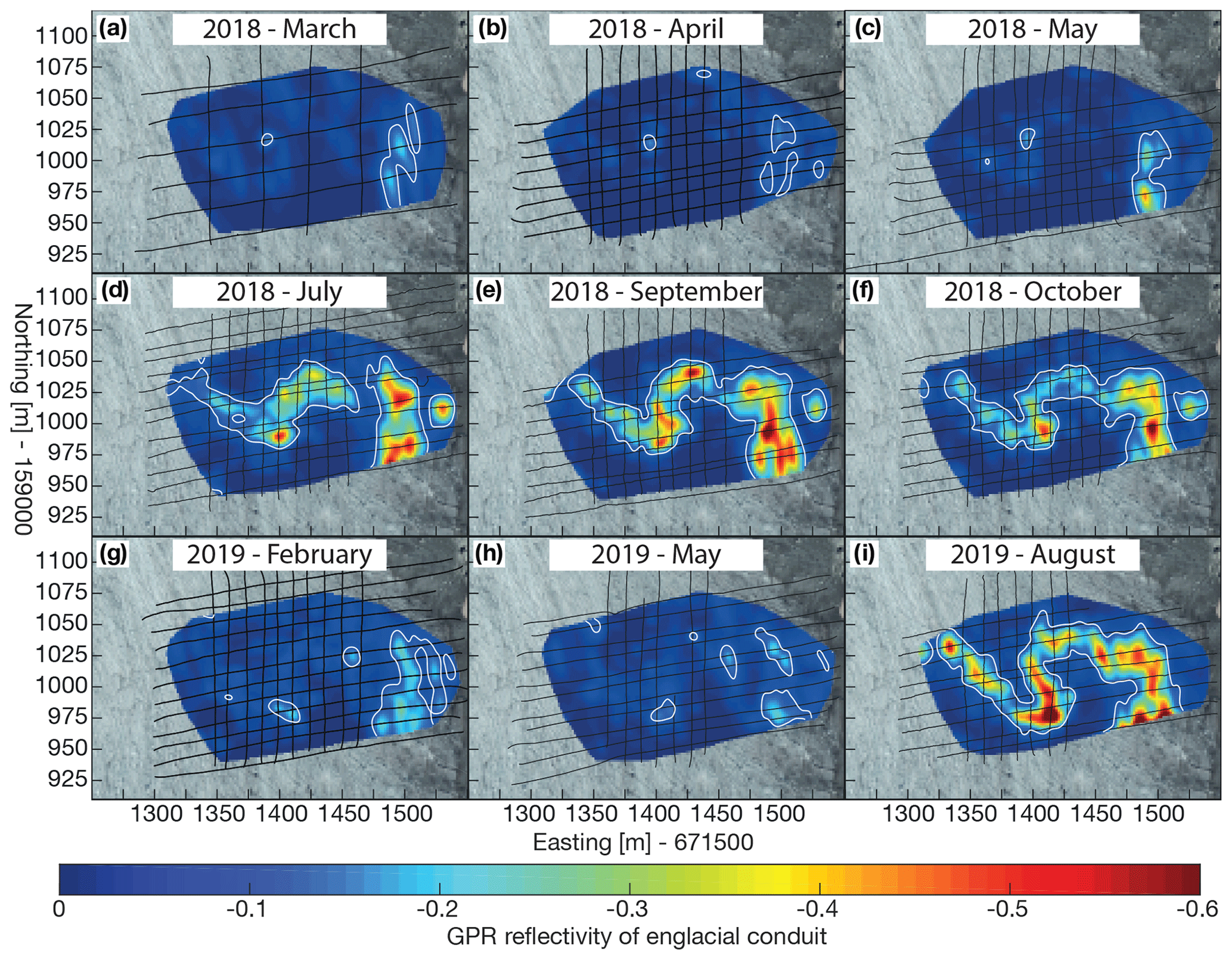
Figure 5Seasonal GPR reflectivity from the top of the englacial channel reflection. The black grid lines represent the GPR acquisition profiles acquired for each month. The white contour represents the reflectivity at −0.1, providing an approximate outline of the englacial conduit.
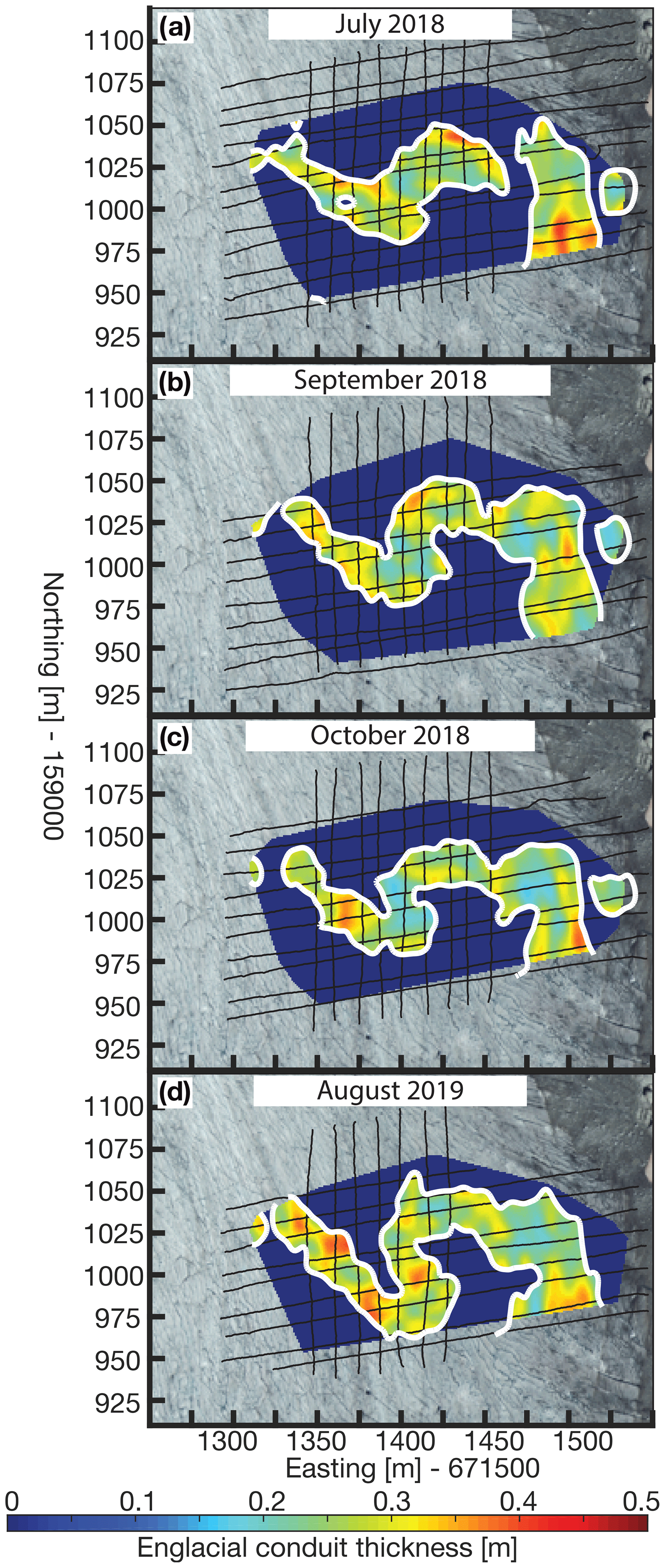
4.4 GPR conduit thickness results
In addition to the seasonal reflectivity results, the conduit thickness was calculated for those surveys, where the top and bottom reflections could be identified. The travel time differences between the top and bottom reflections were converted to thickness using the velocity of an EM wave travelling through water (0.0333 m ns−1). Figure 3g and i show a negative reflectivity for the top of the conduit (red arrows) and a positive reflectivity for the bottom of the conduit (blue arrows). Upon extraction of the conduit thickness, the spatial extent of the conduit thickness was determined by interpolating between the GPR profiles and smoothing (Fig. 6). The conduit thickness is between 0.2 and 0.5 m throughout the melt season (Fig. 6), and there is little variability in the conduit thickness throughout the summer. We performed a thin-layer forward modelling investigation, with which we tried to appraise the reliability and robustness of the thickness estimates.
5.1 Thin channel water layer GPR forward modelling methodology
Reynolds (2011) states that, in theory, the vertical resolution of a GPR signal is a quarter wavelength, assuming the source wavelet is two half cycles. This theory is based upon the seismic wave propagation theory as described by Widess (1973). In reality the GPR source wavelet is typically longer than a single wavelength. With this being the case, the vertical resolution is reduced as a result of the complex nature of the transmitted GPR source wavelet (Reynolds, 2011). For an EM wave propagating within a water-filled conduit the wavelength of a 25 MHz system is 1.333 m, and therefore the theoretical vertical resolution (λ∕4) for a conduit filled with water using 25 MHz antennas is 0.33 m. The true conduit thickness can be determined from the reflectivity inversion if the thickness of the conduit is larger than the theoretical vertical resolution. The thicknesses shown in Fig. 6 are thus within proximity of the theoretical vertical resolution limit.
A forward modelling approach was adopted in order to investigate how a thin water-filled channel layer, below the theoretical vertical resolution, affects the thickness and reflectivity that we recover from the processing workflow described in Table 2. From this point the thickness and reflectivity derived from the modelled GPR data are known as the apparent thickness and reflectivity, whereas the known model thickness and known ice–water reflectivity are known as the true thickness and reflectivity. We generated synthetic radargrams using the open-source software gprMax (Warren et al., 2016). This is a finite-difference time-domain solver for EM wave propagation. We employed a simple 3D model, as sketched in Fig. 7a. It includes a single thin water-filled conduit that is invariable in the third dimension. The associated material parameters are summarised in Table 4. All four boundaries of the model had absorbing boundary conditions in order to prevent multiple energy interfering with the top and bottom reflection from the conduit. The synthetic GPR data (Fig. 7b) were modelled using transmitting and receiving antennas separated by 2 m, and they were moved from 2 to 18 m along the x axis in Fig. 7a at 0.5 m increments. The model space did not contain a free surface in order to have a clear interpretation of the top and bottom conduit reflectors without any multiple energy being present. The numerical simulations and thickness extraction procedures were repeated with a range of conduit thicknesses between 0.05 and 2 m.
Noise-free simulations were initially performed, but for uncertainty analysis coherent noise was added prior to migration. The coherent noise was extracted from the GPR field data acquired in July 2018, and it was added directly to the synthetic data. The synthetic GPR with coherent real noise can be directly compared with the field data in order to make conduit thicknesses and reflection strength deductions. In order to determine how the coherent noise affects the apparent reflectivities and thickness, we used 48 different noise types and performed statistical analysis to determine uncertainties.
5.2 Thin channel water layer GPR forward modelling results
The synthetic GPR data with an example of coherent noise added, shown in Fig. 7b, were generated with a 2 m thick water-filled englacial conduit, and the red and blue arrows represent the reflection from the top and bottom of the conduit respectively. There is a 120 ns separation between the top and bottom reflections (red and blue arrows in Fig. 7) from the conduit using a 2 m thick englacial conduit model, but, as shown in Fig. 8, these two reflectors interfere with each other when the conduit thickness reaches the vertical resolution (0.3 m in Fig. 8). The horizontal width of the water-filled conduit remained at 5 m for all tests and is below the horizontal resolution after migration. In order to extract the reflectivity (Figs. 7c and 8b) from the synthetic GPR data, the data were processed using an identical processing workflow, as applied to the field data.
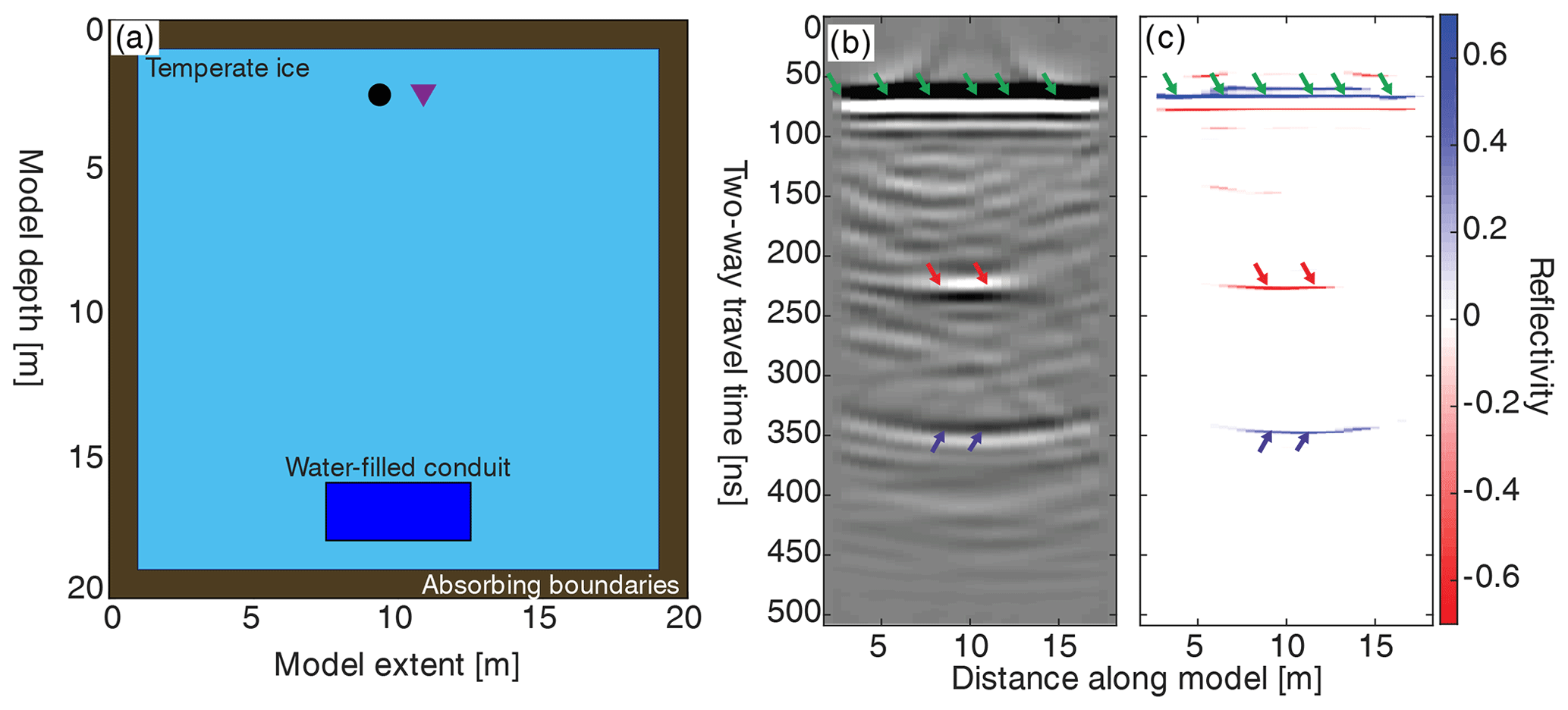
Figure 7Forward modelling results. (a) Geometry model for gprMax forward modelling with temperate ice, a 2 m thick water-filled conduit, and absorbing boundaries labelled. The circle and the triangle represent the transmitting and receiving antennas. (b) The processed synthetic data generated from the model in (a) after step 10 in Table 2. (c) The reflectivity from the data (b) after processing through the entire workflow described in Table 2. The green arrows represent the direct arrival, and the red and blue arrows represent the top and bottom reflections from the englacial conduit respectively.
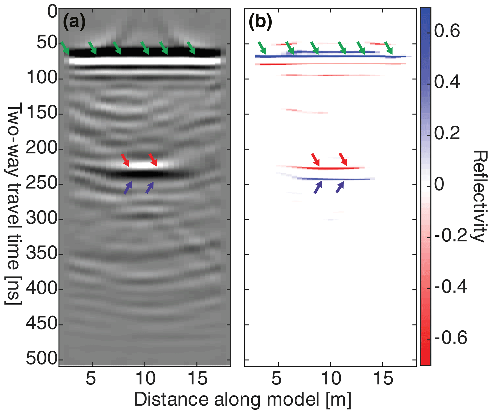
Figure 8Forward modelling results for 0.3 m water-filled conduit. (a) The processed synthetic data after step 10 in Table 2. (b) The reflectivity from the data (a) after processing through the entire workflow described in Table 2. The green arrows represent the direct arrival, and the red and blue arrows represent the interfering top and bottom reflection from the englacial conduit respectively.
The results on the apparent channel thickness as a function of the true model channel thickness are shown in Fig. 9a. We were able to resolve the true conduit thickness of the conduit from the GPR data, when the true thickness was greater than 0.4 m (0.3λ). However, when a water-filled conduit was less than 0.4 m thick, the apparent thickness from the inversion was within ±0.15 m (yellow shaded area in Fig. 9a). In the summer, the majority of the Rhonegletscher imaged englacial conduit network is less than 0.4 m (Fig. 6), and therefore the conduit thickness from Rhonegletscher does not represent the true thickness, but the apparent thickness is within ±0.15 m of the true conduit thickness. The error bars show the effect of the coherent noise added into the model. There is little effect on the thickness estimation with coherent noise added to the model.
In addition to the discrepancies between apparent channel thickness and true channel thickness (Fig. 9a), the GPR zero-offset reflectivity can be analysed as a function of channel thickness (Fig. 9b). An ice–water reflection coefficient is −0.67 and is represented by the pink line in Fig. 9b. For the noise-free data the apparent reflectivity is represented by the red line in Fig. 9b. In order for the conduit top to have an ice–water reflectivity of −0.67 (Table 3), using noise-free data, the conduit must be greater than 0.6 m thick (0.45λ), as represented by the green shaded area in Fig. 9b. With the addition of coherent noise in the simulations, the uncertainty for true thicknesses above 0.6 m is ±0.1. When the conduit is between 0.1 and 0.6 m thick (0.07λ–0.45λ), the noise-free apparent reflectivity is equal to the true reflectivity ±0.1 (shaded yellow area in Fig. 9b). With the addition of the coherent noise to the simulations, the uncertainty doubles to ±0.2. When the conduit is thinner than 0.1 m, the apparent reflectivity is below 0.5 (shaded red area in Fig. 9b). From these results, a likely explanation for the low reflectivities observed from the conduit (Fig. 5) could be the result of the conduit being below the vertical resolution.
Table 4Material properties for the forward modelling, taken from Plewes and Hubbard (2001), Reynolds (2011), and Langhammer et al. (2017). The values within the brackets represent the range of uncertainty.
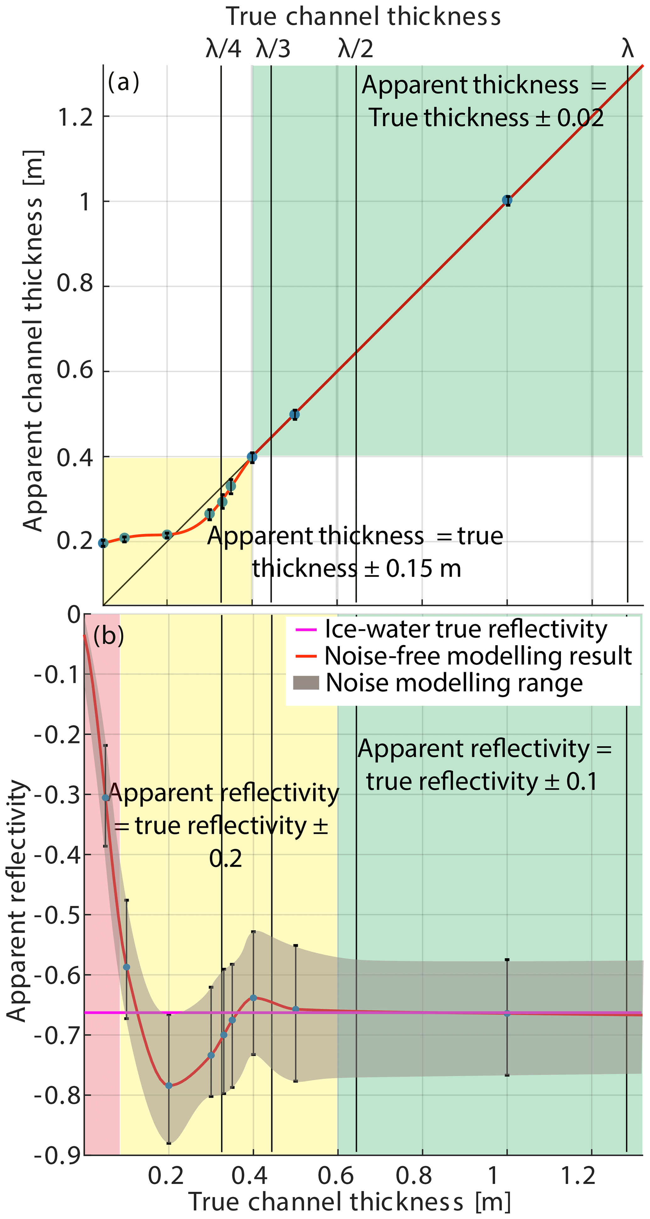
Figure 9Forward modelling apparent thickness and reflectivity results plotted against the true model conduit thickness. (a) The apparent thickness in the GPR inversion processing as a function of the true channel thickness in the model (Fig. 7a using 25 MHz antennas). (b) The apparent reflectivity from the englacial conduit top as a function of the true channel thickness. The error bars represent the 2 standard deviations around 48 different noise records added to the synthetic.
6.1 Uncertainties
6.1.1 EM wave propagation velocities
The EM wave propagation velocity for the four CMPs had a maximum uncertainty of ±0.1 m ns−1, and the mean EM wave-propagating velocity was 0.1675 m ns−1. The EM wave propagation velocities within ice is a function of water content, and quoted values in literature lie between 0.167 and 0.169 m ns−1 (Fujita et al., 2000; Murray et al., 2000; Plewes and Hubbard, 2001; Reynolds, 2011; Bradford et al., 2013). Therefore the EM wave propagation velocity was kept constant for all GPR migrations at 0.1689 m ns−1 and time-to-depth conversions.
6.1.2 Conduit reflectivity
In order to evaluate the reflectivity uncertainty of the field GPR data, we acquired four coincident profiles in a single day in July 2018 and compared their reflectivity results from the GPR processing flow. There is some natural variation in the englacial reflectivity that is likely caused by a combination of minor changes in the walking path leading to different imaging points and differences in the coherent noise. From these repeated measurements the variability has been quantified to be ±0.15 (Fig. S3).
In addition to the field data, an estimate of the channel reflectivity uncertainty was completed using the synthetic testing, when adding coherent noise. The uncertainty on the reflectivity using coherent noise within the numerical modelling is ±0.2 independent of the conduit thickness (grey shaded area in Fig. 9). Both of these errors provide similar uncertainty ranges, and therefore the uncertainty on the apparent reflectivity is estimated to be ±0.2.
Furthermore, GPR reflection coefficients are a function of the incidence angles. As the GPR antennas were constantly separated by 4 m, and the target was around 80–100 m below the glacier surface, the angle of incidence is less than 1∘, and vertically incident waves were therefore assumed for all reflectivity analysis.
6.1.3 Conduit thickness
The uncertainty in the true channel thickness is a function of the picked two-way time, the EM wave propagation velocity through the conduit filling material, and the apparent thickness. Our borehole camera observations provided evidence that the filling material is water (see Supplement video), and there are small amounts of loose sediments. Therefore, an EM wave propagation velocity of fresh water (0.0333 m ns−1) was employed for the time-to-thickness conversion. The small quantity of sediment could potentially increase the EM-propagation velocity. As far as we are aware, there are no studies providing the EM wave velocity through water with a small quantity of sediment. A fully saturated till layer within the conduit would alter the propagation velocity to be within 0.05–0.06 m ns−1 (Reynolds, 2011). Given the borehole observations, it can be safely assumed that the EM-propagating velocities are between 0.033 and 0.05 m ns−1. Therefore, we have attributed a lower-bound uncertainty of 50 % to the apparent thickness related to the time-to-thickness conversion velocity. An upper bound of 0 % exists for the velocity error as the lowest potential velocity within an englacial conduit is the EM-wave propagation velocity through water.
The picking error is within a sample range (1 ns) as a result of picking the reflectivity (Fig. 3g) and not the actual GPR wavelet (Fig. 3c). This small picking error in time equates to only a 1.5 cm error in the conduit thickness and is therefore not a large source of uncertainty and can be neglected.
The GPR forward modelling exercise provided evidence that when the true channel thicknesses were below 0.4 m, the apparent thickness does not represent the true conduit thickness (Fig. 9a). For true conduit thicknesses less than 0.4 m the apparent thickness is within 0.15 m of the true model (40 % error). Conversely, when apparent thicknesses are above 0.4 m they represent the true model, and therefore there is no significant error.
Compounding the conduit thickness uncertainties for apparent conduit thickness below 0.4 m, we have large errors (lower bound: −90 %, upper bound: +40 %). Conversely, for apparent conduit thickness greater than 0.4 m the uncertainty is only a function of the filling EM-propagating velocity (lower bound: −50 %, upper bound: apparent conduit thickness). Despite these relatively large errors, we are able to confidently state the englacial conduit on Rhonegletscher is still a thin layer and below the wavelength of the GPR signal.
6.1.4 Horizontal resolution
The first Fresnel zone defines the horizontal resolution (the ability to distinguish two closely laterally separated reflectors) for GPR. The first Fresnel zone is approximately 17 m for the geometry of our reflector (90 m depth) with a 25 MHz GPR system and the EM wave propagation velocity through ice (0.1689 m ns−1). The GPR data have been migrated using a 2D Kirchhoff migration algorithm, and therefore within the profile the first Fresnel zone is reduced to the bin size (0.5 m). However, the Fresnel zone out of the GPR plane remains 17 m. The acquisition of the GPR was set up to have profiles along and perpendicular to the glacier flow. Acquiring profiles in these orientations ensured that we have a horizontal resolution of 0.5 m in both directions in order to delineate the englacial conduit network. There is an uncertainty of the spatial extent as a result of the linear interpolation of the reflectivities. The spacing between profiles is approximately 12 m, and therefore we would estimate that the uncertainty is around half the profile spacing (6 m).
6.2 Conduit geometry
6.2.1 Conduit extension
During the melt season (July–October), when the englacial conduit is active, the conduit is around 250 m±0.6 m in length and between 20 and 45 m±0.6 m wide. During all the summer acquisitions, the englacial conduit thickness was estimated to be between 0.2 and 0.4 m, exhibiting little variability (Fig. 6). Therefore, the conduit was far wider than its thickness, and it does not follow the typical cylindrical englacial conduit cross-sectional shape, as observed in other GPR surveys (Stuart, 2003), or as described by englacial conduit theory (Shreve, 1972; Roethlisberger, 1972).
6.2.2 Conduit inclination
There is a 10 m global elevation difference in the conduit's topography (Fig. 10) across the entire imaged englacial conduit network, thereby indicating that the conduit has a low inclination (approximately 2∘). The inclination is similar to englacial conduit drainage networks found on a cold-ice glacier in Svalbard (Stuart, 2003; Hansen et al., 2020). Such a small dip provides evidence that the movement of englacial water is not related with the hydraulic gradients and therefore does not support the englacial conduit formation models described by Shreve (1972), which postulates englacial conduit formation through upward branching of an arborescent network.
6.2.3 Conduit shape
The shape of the englacial conduit shows a meandering and sinusoidal outline that runs perpendicular to the ice flow direction. The outline (white contour in Fig. 6) has similar geometry to subsections of englacial conduits that have been mapped using speleology within cold glaciers (Gulley et al., 2009a), which have been formed as a result of the cut-and-closure mechanism. A cut-and-closure englacial conduit forms as a result of surface streams or streams within crevasses incising towards the glacier bed and subsequently becoming isolated from the surface as the ice flows due to ice creep (Fountain and Walder, 1998). Similarly, a sinusoidal shape could result from turbulent water flowing englacially. To the best of our knowledge this is the first example of a temperate glacier to have an active englacial system surveyed using geophysical techniques and showing a sinusoidal shape.
6.3 Conduit formation
The conduit's sinusoidal shape provides some evidence that this englacial drainage system could be the result of a cut-and-closure drainage system. However this hypothesis can be ruled out, as no large visible supraglacial stream has been observed on Rhonegletscher within the proximity of the englacial conduit in previous years. Moreover, comparing the conduit's profile and cross sections with those described by Gulley et al. (2009a) and summarised in Fig. 2 in their publication, the likely formation mechanism is extensional hydrofracturing. Hydrofracturing on extensional stressed glacial ice provides a horizontal profile (shallow dip) and an englacial conduit cross section that is thin and wide. Such extensional stresses may result from the ice flow turning at the survey site towards the proglacial lake. As discussed in Church et al. (2019), the drainage network is likely fed from numerous streams running along the glacier margin and from the surrounding moraine. Additionally, the hydrofracturing can be supported by the fact that periods of high water pressure were observed as a result of the borehole expelling water 3–4 m above the glacier surface in August 2018 (Fig. S5).
We were unable to determine the englacial water flow direction from either the GPR data or the borehole camera. Tracer studies might be an option (Hooke and Pohjola, 1994; Hock et al., 1999). Unfortunately, this would be difficult, as the studied englacial network is expected to flow into the proglacial lake, and therefore monitoring the tracer quantity would require samples to be taken directly from a borehole instead of an outflow stream from the glacier's tongue.
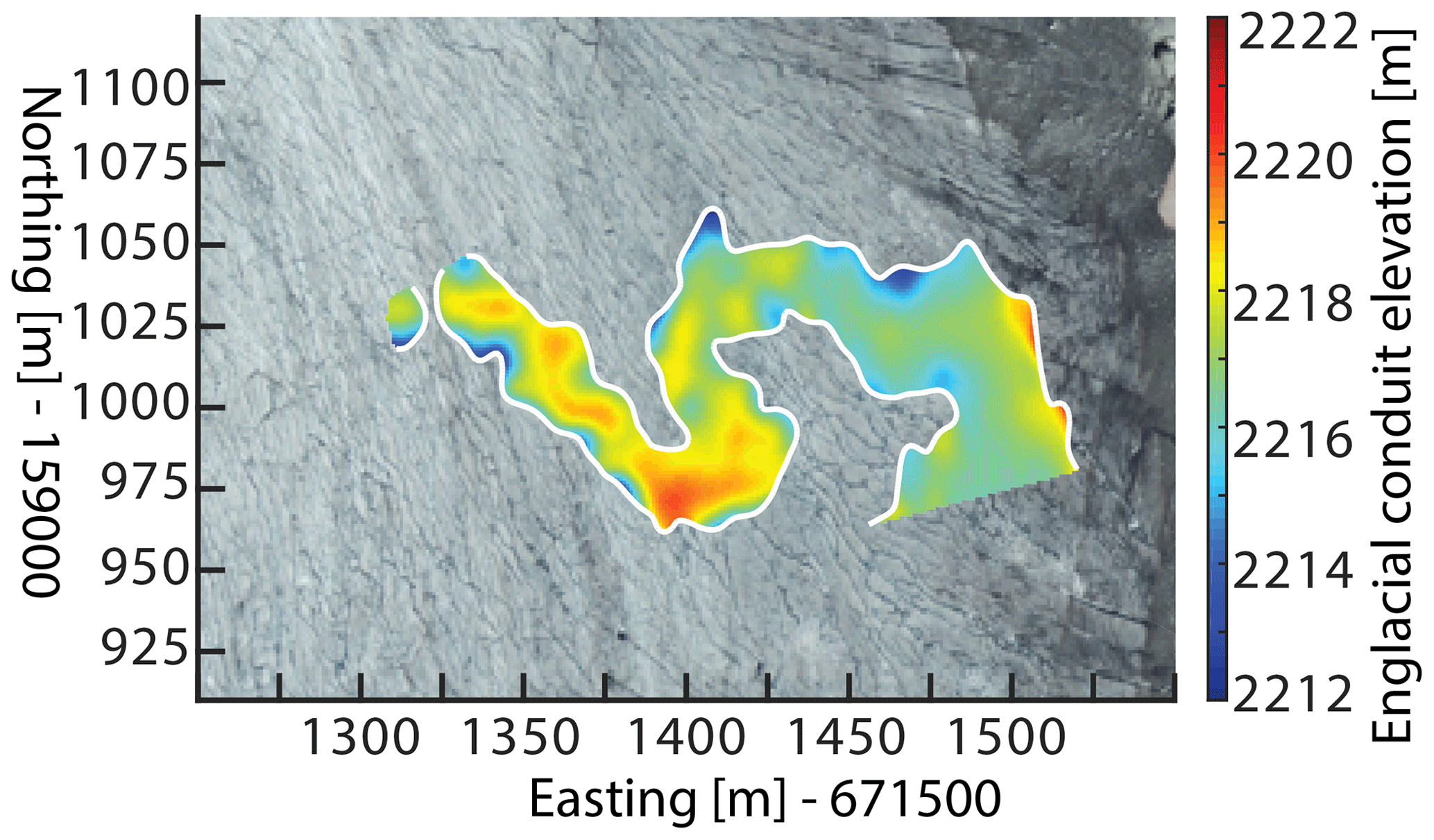
Figure 10Elevation above mean sea level from the top of the englacial conduit network in August 2019.
6.4 Conduit's seasonal variations
The conduit morphology alters throughout the year as a result of the varying discharge from the glacier. Theory states that a steady-state englacial conduit, where the opening rate equals the conduit closure rate, the size and shape of the conduit remains constant (Cuffey and Paterson, 2010). Changes in water supply can alter the opening and closure rates and thereby alter the conduit's morphology. Englacial conduits can shrink and disappear, when discharge quantities are low, whereas high discharge rates can cause a conduit to expand. Runoff and discharge data are available at a gauging station in Gletsch (1800 m a.s.l.), 2 km downstream from Rhonegletscher (Fig. S4). The peak discharge occurs annually between 24 July and 17 August. The end of the peak discharge correlates with the time of the year, where the conduit was well developed in 2019 (Fig. 6d). We can speculate that during August, when there is peak discharge, the englacial network is at its maximum observed extent.
There exists a winter shutdown of the englacial conduit network between 2018 and 2019, indicated by a near-zero reflectivity (Fig. 5e). Remnants of the englacial conduit are detectable on the winter reflectivity, when restricting the colour scale from −0.05 to −0.15 (Fig. 11, grey line). If the conduit is fully open (thickness >0.5 m), then it is neither water nor air filled during the winter as a large negative reflectivity (ice–water: −0.67) or positive reflectivity (ice–air: +0.3) is not observed. During August 2018, we were able to make direct borehole measurements using a borehole camera and observed sediment being transported along the base of the conduit (see video Supplement S1). Therefore, as a result of the lower reflectivity and the lower discharge, we speculate that during winter the conduit either physically closes or becomes very thin (<0.1 m) and remains water filled. If the conduit physically closes, the sediments lying within the closed conduit are likely the cause of the low winter reflectivity, and the reflectivity values around −0.1 would indicate an englacial environment without the presence of water. Conversely, if the conduit thinned to less than 0.1 m and remained water filled, the reflectivity values are around −0.1 (red area in Fig. 9b). The repeated GPR summer measurements in 2018 and 2019 provided evidence that the conduit networks reopen in an identical location. In order for the conduit to be reactivated during the 2019 melt season, either the sediments lying within the closed conduit during the winter months provided a potential permeable flow path in 2019 or the englacial conduit remained connected after becoming a very thin water-filled (<0.1 m) conduit during the winter. Furthermore, we speculate that the hydraulic potential is similar during both melt seasons as the englacial conduit is reactivated in an identical position after the winter shutdown.
The GPR wavelet character from the conduit's top remains a constant negative high-amplitude reflector over the three melt seasons (2017, 2018, and 2019), which indicates the presence of water within the system during our GPR summer acquisitions. From the GPR data, we are able to determine that the englacial conduit network is above atmospheric pressure. If the system were at atmospheric pressure, the top reflector would be an interface between ice and air and result in a positive-amplitude reflector. Such an unpressurised englacial network was observed by Stuart (2003), where the conduit's top reflection was a high-positive-amplitude reflector. The fact that the conduit is above atmospheric pressure is additionally supported by our borehole camera observations, where the borehole water level was 1–2 m above the englacial network during observations, suggesting that the water pressure was slightly above atmospheric pressure.

Figure 11Winter GPR reflectivity from the top of the englacial channel reflection plotted between 0 and −0.15 reflectivity values, highlighting remnants of the englacial conduit network that exist during the winter months. The grey line represents the summer englacial conduit shape. The black grid lines represent the GPR acquisition profiles acquired for each month. The white contour represents the reflectivity at −0.05.
6.5 General applicability and limitations of GPR to characterise englacial conduits
So far, there exist a few studies, where englacial conduits have been characterised using a combination of GPR with speleology or borehole observations (Moorman and Michel, 2000; Stuart, 2003; Catania et al., 2008; Temminghoff et al., 2019; Schaap et al., 2019). In these studies, englacial conduits were imaged as point diffractors. Without speleology or boreholes, the interpretation of these point diffractors is typically ambiguous. In the Rhonegletscher case study, the interpretation is unambiguous with the ground-truth borehole observations, because the englacial conduit appears as a single specular reflection.
For future studies investigating englacial conduits, the GPR reflectivity workflow can be used to identify englacial conduits and conditions on the glacier's bed, but it is essential to calibrate the apparent reflectivities with known reflectivities on site. As far as we are aware, there is no such reflectivity analysis for glacial drainage networks on temperate glaciers. For the Rhonegletscher data, this was obtained from borehole observations. However, for other studies, a known reflectivity point may not be available in order to calibrate the reflectivity, and therefore by plotting the uncalibrated reflectivity of an englacial reflector, potential flow paths could be delineated. However the filling material would remain unknown. Such an approach was adopted in Bælum and Benn (2011) (plotting the reflection-normalised amplitude of the glacier's bed). The workflow could be extended to specular glacier basement reflectors in order to detect subglacial conduit networks. However, the GPR processing workflow does not correct for the anisotropic GPR radiation pattern. In this case, dipping specular reflectors will have amplitudes dependent on both the radiation pattern and the angle-dependent reflection coefficient. Therefore an extension of the workflow needs to be made, and a migration accounting for GPR antenna radiation pattern needs to be implemented prior to the impedance inversion in order to extract the reflectivity coefficient.
This study has also provided evidence that the glacier's bed needs to be interpreted with care. The Rhonegletscher case study has identified an englacial conduit as a specular reflector 10–15 m above the glacier's bed during the melt season. If a single GPR profile would have been acquired during the melt season (e.g. August 2019, Fig. 3e), the englacial conduit may have been misinterpreted as the glacier bed. Therefore, it is essential to understand the hydrological conditions of the glacier, when designing GPR surveys in order to successfully interpret the GPR data. For GPR surveys, where the ice thickness is the objective on temperate alpine glaciers, then GPR acquisition should be undertaken during winter in order to minimise the englacial water-storage-limiting penetration depth. Conversely, for GPR surveys investigating the glacier's hydrological conditions it is intuitive that acquisition should take place during summer.
From the forward modelling, the vertical resolution for GPR was found to be 0.3λ. If two interfaces are spaced less than 0.3λ m vertically apart, then there is interference between the two reflectors, which leads to an erroneous thickness interpretation (Fig. 9). This GPR vertical resolution is larger than seismic vertical resolution found through forward modelling on ice–water reflectivities (King et al., 2004), as a result of the complex nature of the GPR source wavelet.
By using repeated GPR measurements and processing the data with an impedance inversion to extract the reflectivity, we have mapped the changing spatial extent and thickness of an active and dynamic englacial conduit network on a temperate glacier. The repeated seasonal GPR measurements in 2018 and 2019 and the reflection coefficient analysis of the englacial conduit provided an insight into the evolution of an active englacial hydrological network.
In summer the englacial conduit was transporting water through the glacier, leading to large negative reflectivity values (). The Rhonegletscher's englacial network followed a meandering and sinusoidal shape throughout the melt season. The conduit is 15–20 m wide and between 0.2 and 0.4 m thick. Such a conduit cross section (wide and thin) can occur as a result of hydraulic fracturing with extensional stresses acting on the ice, based upon the englacial conduit shape review by Gulley et al. (2009a). Furthermore, water flowing through the englacial conduit during the melt season feeds the subglacial drainage network, which likely increases subglacial water pressure and facilitates basal sliding.
The englacial conduit was found to have reduced in thickness and was not transporting water during the winter period, with reflectivity values between −0.05 and −0.15. Therefore, we speculate that during the winter the conduit network either physically closes or is very thin (<0.1 m). Either, sediments that were being transported within the conduit in the summer or water within a thin-layer conduit are likely responsible for the reflectivity visible during the winter GPR acquisition. The englacial conduit became active in an identical location after a winter shutdown. The conduit's shape remained similar in the winter compared to the summer.
Difficulties arise when interpreting a series of reflectors that are separated by the vertical resolution. The forward modelling has shown that two horizons are perfectly distinguishable when they are separated by more than 0.3λ. Conversely, the amplitude or reflectivity of the top interface is only resolved when the thickness is greater than 0.45λ. We conclude that care must be taken when inferring material properties from a reflectivity processing workflow with the presence of thin layers that approach the vertical resolution of the GPR source wavelet.
Movie S1 https://doi.org/10.3929/ethz-b-000406689 (Church, 2020) shows the borehole camera observations made directly into the active englacial conduit on 24 July 2018.
The supplement related to this article is available online at: https://doi.org/10.5194/tc-14-3269-2020-supplement.
GC, MG, AB, and HM designed the GPR experiments, which were carried out by GC and MG. GC processed the data with help from CS, and all authors analysed the data. GC interpreted the data with help from all co-authors. GC wrote the manuscript with contributions from all co-authors.
The authors declare that they have no conflict of interest.
Data acquisition has been provided by the Exploration and Environment Geophysics (EEG) group and the Laboratory of Hydraulics, Hydrology and Glaciology (VAW) of ETH Zurich. We would like to gratefully acknowledge the Landmark Graphics Corporation for providing data processing software through the Landmark University Grant Program. The authors wish to acknowledge all volunteers for their valuable help in the fieldwork. We would like to thank the editor, Nanna Bjørnholt Karlsson, and the two reviewers, Slawek Tulaczyk and Ugo Nanni, for their constructive comments in order to improve the quality of the manuscript.
This research has been supported by the Schweizerischer Nationalfonds zur Förderung der Wissenschaftlichen Forschung (grant no. 200021_169329/1).
This paper was edited by Nanna Bjørnholt Karlsson and reviewed by Ugo Nanni and Slawek Tulaczyk.
Arcone, S. A. and Yankielun, N. E.: 1.4 GHz radar penetration and evidence of drainage structures in temperate ice: Black Rapids Glacier, Alaska, U.S.A., J. Glaciol., 46, 477–490, https://doi.org/10.3189/172756500781833133, 2000. a
Arcone, S. A., Lawson, D. E., and Delaney, A. J.: Short-pulse radar wavelet recovery and resolution of dielectric contrasts within englacial and basal ice of Matanuska Glacier, Alaska, U.S.A., J. Glaciol., 41, 68–86, https://doi.org/10.1017/S0022143000017779, 1995. a
Bælum, K. and Benn, D. I.: Thermal structure and drainage system of a small valley glacier (Tellbreen, Svalbard), investigated by ground penetrating radar, The Cryosphere, 5, 139–149, https://doi.org/10.5194/tc-5-139-2011, 2011. a, b
Bartholomaus, T. C., Amundson, J. M., Walter, J. I., O'Neel, S., West, M. E., and Larsen, C. F.: Subglacial discharge at tidewater glaciers revealed by seismic tremor, Geophys. Res. Lett., 42, 6391–6398, https://doi.org/10.1002/2015GL064590, 2015. a
Benn, D., Gulley, J., Luckman, A., Adamek, A., and Glowacki, P. S.: Englacial drainage systems formed by hydrologically driven crevasse propagation, J. Glaciol., 55, 513–523, https://doi.org/10.3189/002214309788816669, 2009. a
Bingham, R. G., Nienow, P. W., Sharp, M. J., and Boon, S.: Subglacial drainage processes at a High Arctic polythermal valley glacier, J. Glaciol., 51, 15–24, https://doi.org/10.3189/172756505781829520, 2005. a
Bingham, R. G., Hubbard, A. L., Nienow, P. W., and Sharp, M. J.: An investigation into the mechanisms controlling seasonal speedup events at a High Arctic glacier, J. Geophys. Res.-Earth Surf., 113, 1–13, https://doi.org/10.1029/2007JF000832, 2008. a
Boon, S. and Sharp, M.: The role of hydrologically-driven ice fracture in drainage system evolution on an Arctic glacier, Geophys. Res. Lett., 30, 3–6, https://doi.org/10.1029/2003GL018034, 2003. a, b
Booth, A. D., Clark, R., and Murray, T.: Semblance response to a ground-penetrating radar wavelet and resulting errors in velocity analysis, Near Surf. Geophys., 8, 235–246, https://doi.org/10.3997/1873-0604.2010008, 2010. a
Bradford, J. H., Nichols, J., Harper, J. T., and Meierbachtol, T.: Compressional and EM wave velocity anisotropy in a temperate glacier due to basal crevasses, and implications for water content estimation, Ann. Glaciol., 54, 168–178, https://doi.org/10.3189/2013AoG64A206, 2013. a
Catania, G. A. and Neumann, T. A.: Persistent englacial drainage features in the Greenland Ice Sheet, Geophys. Res. Lett., 37, 1–5, https://doi.org/10.1029/2009GL041108, 2010. a
Catania, G. A., Neumann, T. A., and Price, S. F.: Characterizing englacial drainage in the ablation zone of the Greenland ice sheet, J. Glaciol., 54, 567–578, https://doi.org/10.3189/002214308786570854, 2008. a, b
Christianson, K., Jacobel, R. W., Horgan, H. J., Alley, R. B., Anandakrishnan, S., Holland, D. M., and DallaSanta, K. J.: Basal conditions at the grounding zone of Whillans Ice Stream, West Antarctica, from ice-penetrating radar, J. Geophys. Res.-Earth Surf., 121, 1954–1983, https://doi.org/10.1002/2015JF003806, 2016. a
Church, G. J.: Borehole Camera Video of Englacial Conduit, ETH Zürich Research Collection, https://doi.org/10.3929/ethz-b-000406689, 2020. a
Church, G., Bauder, A., Grab, M., Rabenstein, L., Singh, S., and Maurer, H.: Detecting and characterising an englacial conduit network within a temperate Swiss glacier using active seismic, ground penetrating radar and borehole analysis, Ann. Glaciol., 60, 193–205, https://doi.org/10.1017/aog.2019.19, 2019. a, b, c, d
Church, G. J., Bauder, A., Grab, M., Hellmann, S., and Maurer, H.: High-resolution helicopter-borne ground penetrating radar survey to determine glacier base topography and the outlook of a proglacial lake, in: 2018 17th International Conference on Ground Penetrating Radar (GPR), pp. 1–4, IEEE, https://doi.org/10.1109/ICGPR.2018.8441598, 2018. a, b
Cuffey, K. M. and Paterson, W. S. B.: The Physics of Glaciers, Fourth Edition, Academic Press, fourth edn., 2010. a, b
Farinotti, D., Huss, M., Bauder, A., and Funk, M.: An estimate of the glacier ice volume in the Swiss Alps, Global Planet. Change, 68, 225–231, https://doi.org/10.1016/j.gloplacha.2009.05.004, 2009. a
Fountain, A. G. and Walder, J. S.: Water flow through temperate glaciers, Rev. Geophys., 36, 299–328, https://doi.org/10.1029/97RG03579, 1998. a, b, c
Fountain, A. G., Jacobel, R. W., Schlichting, R., and Jansson, P.: Fractures as the main pathways of water flow in temperate glaciers, Nature, 433, 618–621, https://doi.org/10.1038/nature03296, 2005. a, b
Fujita, S., Matsuoka, T., Ishida, T., Matsuoka, K., and Mae, S.: A summary of the complex dielectric permittivity of ice in the megahertz range and its applications for radar sounding of polar ice sheets, Physics of Ice Core Records, pp. 185–212, 2000. a
Gimbert, F., Tsai, V. C., Amundson, J. M., Bartholomaus, T. C., and Walter, J. I.: Subseasonal changes observed in subglacial channel pressure, size, and sediment transport, Geophys. Res. Lett., 43, 3786–3794, https://doi.org/10.1002/2016GL068337, 2016. a
Glen, J. W. and Paren, J. G.: The Electrical Properties of Snow and Ice, J. Glaciol., 15, 15–38, https://doi.org/10.3189/S0022143000034249, 1975. a
Grab, M., Bauder, A., Ammann, F., Langhammer, L., Hellmann, S., Church, G., Schmid, L., Rabenstein, L., and Maurer, H.: Ice volume estimates of Swiss glaciers using helicopter-borne GPR an example from the Glacier de la Plaine Morte, in: 2018 17th International Conference on Ground Penetrating Radar (GPR), pp. 1–4, IEEE, https://doi.org/10.1109/ICGPR.2018.8441613, 2018. a
Gulley, J.: Structural control of englacial conduits in the temperate Matanuska Glacier, Alaska, USA, J. Glaciol., 55, 681–690, https://doi.org/10.3189/002214309789470860, 2009. a, b, c
Gulley, J. and Benn, D. I.: Structural control of englacial drainage systems in Himalayan debris-covered glaciers, J. Glaciol., 53, 399–412, https://doi.org/10.3189/002214307783258378, 2007. a
Gulley, J., Benn, D., Müller, D., and Luckman, A.: A cut-and-closure origin for englacial conduits in uncrevassed regions of polythermal glaciers, J. Glaciol., 55, 66–80, https://doi.org/10.3189/002214309788608930, 2009a. a, b, c, d, e
Gulley, J., Benn, D., Screaton, E., and Martin, J.: Mechanisms of englacial conduit formation and their implications for subglacial recharge, Quaternary Sci. Rev., 28, 1984–1999, https://doi.org/10.1016/j.quascirev.2009.04.002, 2009b. a
Guo, L., Chen, J., and Lin, H.: Subsurface lateral preferential flow network revealed by time-lapse ground-penetrating radar in a hillslope, Water Resour. Res., 50, 9127–9147, https://doi.org/10.1002/2013WR014603, 2014. a
Hansen, L., Piotrowski, J., Benn, D., and Sevestre, H.:. A cross-validated three-dimensional model of an englacial and subglacial drainage system in a High-Arctic glacier, J. Glaciol., 66, 278–290, https://doi.org/10.1017/jog.2020.1, 2020. a, b
Hart, J. K., Rose, K. C., Clayton, A., and Martinez, K.: Englacial and subglacial water flow at Skálafellsjökull, Iceland derived from ground penetrating radar, in situ Glacsweb probe and borehole water level measurements, Earth Surf. Proc. Land., 40, 2071–2083, https://doi.org/10.1002/esp.3783, 2015. a
Hewitt, I. J.: Seasonal changes in ice sheet motion due to melt water lubrication, Earth Planet. Sc. Lett., 371-372, 16–25, https://doi.org/10.1016/j.epsl.2013.04.022, 2013. a
Hock, R., Iken, L., and Wangler, A.: Tracer experiments and borehole observations in the over-deepening of Aletschgletscher, Switzerland, Ann. Glaciol., 28, 253–260, https://doi.org/10.3189/172756499781821742, 1999. a, b
Hooke, R. L. and Pohjola, V. A.: Hydrology of a segment of a glacier situated in an overdeepening, Storglaciaren, Sweden, J. Glaciol., 40, 140–148, 1994. a
Huss, M. and Farinotti, D.: Distributed ice thickness and volume of all glaciers around the globe, J. Geophys. Res.-Earth Surf., 117, 1–10, https://doi.org/10.1029/2012JF002523, 2012. a
Iken, A. and Bindschadler, R. A.: Combined measurements of Subglacial Water Pressure and Surface Velocity of Findelengletscher, Switzerland: Conclusions about Drainage System and Sliding Mechanism, J. Glaciol., 32, 101–119, https://doi.org/10.3189/S0022143000006936, 1986. a
Iken, A., Fabri, K., and Funk, M.: Water storage and subglacial drainage conditions inferred from borehole measurements on Gornergletscher, Valais, Switzerland, J. Glaciol., 42, 233–245, 1996. a
Irvine-Fynn, T. D. L., Moorman, B. J., Williams, J. L. M., and Walter, F. S. A.: Seasonal changes in ground-penetrating radar signature observed at a polythermal glacier, Bylot Island, Canada, Earth Surf. Proc. Land., 31, 892–909, https://doi.org/10.1002/esp.1299, 2006. a
King, E. C., Woodward, J., and Smith, A. M.: Seismic evidence for a water-filled canal in deforming till beneath Rutford Ice Stream, West Antarctica, Geophys. Res. Lett., 31, 4–7, https://doi.org/10.1029/2004GL020379, 2004. a
Langhammer, L., Rabenstein, L., Bauder, A., and Maurer, H.: Ground-penetrating radar antenna orientation effects on temperate mountain glaciers, Geophysics, 82, H15–H24, https://doi.org/10.1190/geo2016-0341.1, 2017. a, b
Lindner, F., Walter, F., Laske, G., and Gimbert, F.: Glaciohydraulic seismic tremors on an Alpine glacier, The Cryosphere, 14, 287–308, https://doi.org/10.5194/tc-14-287-2020, 2020. a
Lliboutry, L.: Permeability, Brine Content and Temperature of Temperate Ice, J. Glaciol., 10, 15–29, https://doi.org/10.1017/S002214300001296X, 1971. a
Macgregor, J. A., Anandakrishnan, S., Catania, G. A., and Winebrenner, D. P.: The grounding zone of the Ross Ice Shelf, West Antarctica, from ice-penetrating radar, J. Glaciol., 57, 917–928, https://doi.org/10.3189/002214311798043780, 2011. a
Mercanton, P. L.: Vermessungen am Rhonegletscher, 1874–1915, Neue Denkschriften der Schweizerischen Naturforschenden Gesellschaft, Zurich, 52, 1916. a
Moorman, B. J. and Michel, F. A.: Glacial hydrological system characterization using ground-penetrating radar, Hydrol. Process., 14, 2645–2667, https://doi.org/10.1002/1099-1085(20001030)14:15<2645::AID-HYP84>3.0.CO;2-2, 2000. a, b
Murray, T., Stuart, G. W., Gamble, N. H., and Crabtree, M. D.: Englacial water distribution in a temperature glacier from surface and borehole radar velocity analysis, J. Glaciol., 46, 389–398, https://doi.org/10.3189/172756500781833188, 2000. a
Naegeli, K., Lovell, H., Zemp, M., and Benn, D. I.: Dendritic subglacial drainage systems in cold glaciers formed by cut-and-closure processes, Geogr. Ann. A, 96, 591–608, https://doi.org/10.1111/geoa.12059, 2014. a
Nanni, U., Gimbert, F., Vincent, C., Gräff, D., Walter, F., Piard, L., and Moreau, L.: Quantification of seasonal and diurnal dynamics of subglacial channels using seismic observations on an Alpine glacier, The Cryosphere, 14, 1475–1496, https://doi.org/10.5194/tc-14-1475-2020, 2020. a
Nienow, P., Sharp, M., and Willis, I.: Temporal Switching Between Englacial and Subglacial Drainage Pathways: Dye Tracer Evidence from the Haut Glacier D'arolla, Switzerland, Geogr. Ann. A, 78, 51–60, https://doi.org/10.1080/04353676.1996.11880451, 1996. a
Nienow, P., Sharp, M., and Willis, I.: Seasonal changes in the morphology of the subglacial drainage system, Haut Glacier d'Arolla, Switzerland, Earth Surf. Proc. Land., 23, 825–843, https://doi.org/10.1002/(SICI)1096-9837(199809)23:9<825::AID-ESP893>3.0.CO;2-2, 1998. a
Pettersson, R., Jansson, P., and Holmlund, P.: Cold surface layer thinning on Storglaciären, Sweden, observed by repeated ground penetrating radar surveys, J. Geophys. Res.-Earth Surf., 108, F1, 6004, https://doi.org/10.1029/2003JF000024, 2003. a
Plewes, L. A. and Hubbard, B.: A review of the use of radio-echo sounding in glaciology, Prog. Phys. Geogr., 25, 203–236, https://doi.org/10.1177/030913330102500203, 2001. a, b
Reynolds, J. M.: An Introduction to Applied and Environmental Geophysics, John Wiley & Sons, Oxford, UK, 2011. a, b, c, d, e, f
Roethlisberger, H.: Seismic Exploration in Cold Regions, U.S. Cold Regions Research and Engineering Laboratory, Hanover, N. H, 1972. a
Röthlisberger, H.: Water Pressure in Intra- and Subglacial Channels, J. Glaciol., 11, 177–203, https://doi.org/10.1017/S0022143000022188, 1972. a
Russell, B. H.: Introduction to Seismic Inversion Methods, Society of Exploration Geophysicists, https://doi.org/10.1190/1.9781560802303, 1988. a
Rutishauser, A., Maurer, H., and Bauder, A.: Helicopter-borne ground-penetrating radar investigations on temperate alpine glaciers: A comparison of different systems and their abilities for bedrock mapping, GEOPHYSICS, 81, WA119–WA129, https://doi.org/10.1190/geo2015-0144.1, 2016. a, b
Sacchi, M. D.: Reweighting strategies in seismic deconvolution, Geophys. J. Int., 129, 651–656, https://doi.org/10.1111/j.1365-246X.1997.tb04500.x, 1997. a, b
Schaap, T., Roach, M. J., Peters, L. E., Cook, S., Kulessa, B., and Schoof, C.: Englacial drainage structures in an East Antarctic outlet glacier, J. Glaciol., https://doi.org/10.1017/jog.2019.92, 2019. a, b
Schmelzbach, C. and Huber, E.: Efficient deconvolution of ground-penetrating radar data, IEEE T. Geosci. Remote, 53, 5209–5217, https://doi.org/10.1109/TGRS.2015.2419235, 2015. a, b
Schmelzbach, C., Tronicke, J., and Dietrich, P.: High-resolution water content estimation from surface-based ground-penetrating radar reflection data by impedance inversion, Water Resour. Res., 48, 1–16, https://doi.org/10.1029/2012WR011955, 2012. a, b, c, d
Shreve, R. L.: Movement of Water in Glaciers, J. Glaciol., 11, 205–214, https://doi.org/10.3189/S002214300002219X, 1972. a, b, c
Stuart, G.: Characterization of englacial channels by ground-penetrating radar: An example from austre Brøggerbreen, Svalbard, J. Geophys. Res., 108, 2525, https://doi.org/10.1029/2003JB002435, 2003. a, b, c, d, e
Temminghoff, M., Benn, D. I., Gulley, J. D., and Sevestre, H.: Characterization of the englacial and subglacial drainage system in a high Arctic cold glacier by speleological mapping and ground-penetrating radar, Geogr. Ann. A, 101, 98–117, https://doi.org/10.1080/04353676.2018.1545120, 2019. a, b
Truss, S., Grasmueck, M., Vega, S., and Viggiano, D. A.: Imaging rainfall drainage within the Miami oolitic limestone using high-resolution time-lapse ground-penetrating radar, Water Resour. Res., 43, 1–15, https://doi.org/10.1029/2005WR004395, 2007. a
Tsutaki, S., Sugiyama, S., Nishimura, D., and Funk, M.: Acceleration and flotation of a glacier terminus during formation of a proglacial lake in Rhonegletscher, Switzerland, J. Glaciol., 59, 559–570, https://doi.org/10.3189/2013JoG12J107, 2013. a
van der Veen, C. J.: Fracture propagation as means of rapidly transferring surface meltwater to the base of glaciers, Geophys. Res. Lett., 34, 1–5, https://doi.org/10.1029/2006GL028385, 2007. a
Vatne, G.: Geometry of englacial water conduits, Austre Brøggerbreen, Svalbard, Norsk Geografisk Tidsskrift, 55, 85–93, https://doi.org/10.1080/713786833, 2001. a, b
Velis, D. R.: Stochastic sparse-spike deconvolution, Geophysics, 73, R1–R9, https://doi.org/10.1190/1.2790584, 2008. a
Vore, M. E., Bartholomaus, T. C., Winberry, J. P., Walter, J. I., and Amundson, J. M.: Seismic Tremor Reveals Spatial Organization and Temporal Changes of Subglacial Water System, J. Geophys. Res.-Earth Surf., 124, 427–446, https://doi.org/10.1029/2018JF004819, 2019. a
Warren, C., Giannopoulos, A., and Giannakis, I.: gprMax: Open source software to simulate electromagnetic wave propagation for Ground Penetrating Radar, Comput. Phys. Commun., 209, 163–170, https://doi.org/10.1016/j.cpc.2016.08.020, 2016. a
Widess, M. B.: How thin is a bed?, Geophysics, 38, 1176–1180, https://doi.org/10.1190/1.1440403, 1973. a
Zwally, H. J., Abdalati, W., Herring, T., Larson, K., Saba, J., and Steffen, K.: Surface melt-induced acceleration of Greenland ice-sheet flow, Science, 297, 218–222, https://doi.org/10.1126/science.1072708, 2002. a
- Abstract
- Introduction
- Study site
- Field data and processing
- Field data results
- Numerical modelling: thin channel water layer GPR forward modelling
- Discussion
- Conclusions
- Video supplement
- Author contributions
- Competing interests
- Acknowledgements
- Financial support
- Review statement
- References
- Supplement