the Creative Commons Attribution 4.0 License.
the Creative Commons Attribution 4.0 License.
 | 22 Sep 2020
Brief communication: Time step dependence (and fixes) in Stokes simulations of calving ice shelves
Jeremy Bassis
The buoyancy boundary condition applied to floating portions of ice sheets and glaciers in Stokes models requires special consideration when the glacier rapidly departs from hydrostatic equilibrium. This boundary condition can manifest in velocity fields that are unphysically (and strongly) dependent on time step size, thereby contaminating diagnostic stress fields. This can be especially problematic for models of calving glaciers, where rapid changes in geometry cause configurations that suddenly depart from hydrostatic equilibrium and lead to inaccurate estimates of the stress field. Here we show that the unphysical behavior can be cured with minimal computational cost by reintroducing a regularization that corresponds to the acceleration term in the stress balance. This regularization provides consistent velocity solutions for all time step sizes.
- Article
(851 KB) - Full-text XML
- BibTeX
- EndNote


Stokes simulations are used in glaciology as a tool to determine the time evolution of glaciers (e.g., Gagliardini et al., 2013). Increasingly, these models are also used to examine the stress field within glaciers to better understand factors that control crevasse formation and the onset of calving events (Ma et al., 2017; Benn et al., 2017; Nick et al., 2010; Todd and Christoffersen, 2014; Ma and Bassis, 2019). This type of model can provide insight into the relationship between calving, climate forcing, and boundary conditions (e.g., Todd and Christoffersen, 2014; Ma et al., 2017; Ma and Bassis, 2019).
Here we show that a common method used to implement the ice–ocean boundary condition in Stokes models can result in solutions that are unphysically sensitive to the choice of simulation time step size. This behavior manifests in applications that allow for rapid changes in the model domain – a type of change associated with models that allow for instantaneous calving events or crevasses (Todd and Christoffersen, 2014; Todd et al., 2018; Yu et al., 2017). The time step dependence arises because for glaciers outside of hydrostatic equilibrium, the acceleration is not small as assumed in Stokes flow. We illustrate both the issue and the solution using an idealized ice shelf geometry (Fig. 1) where the upper portion has calved away, emulating the “footloose” mechanism proposed by Wagner et al. (2014) where an aerial portion of the calving front first detaches.
2.1 Glacier stress balance
Denoting the velocity field in two dimensions by and pressure by , conservation of linear momentum can be written in the form
where D∕Dt denotes the material derivative. The Cauchy stress is defined in terms of strain rate, effective viscosity, pressure, and the identity matrix I:
with strain rate tensor ϵ given by
Here ρi is the density of ice, g is the acceleration due to gravity, and η is the effective viscosity of ice:
The effective viscosity is a function of the effective strain rate , a temperature-dependent constant B, and the flow-law exponent n=3.
In the Stokes approximation, we drop the acceleration term on the right-hand side of Eq. (1), which is justified for most glaciological applications (e.g., Greve and Blatter, 2009). However, as we shall show, this assumption is problematic for applications where the ice rapidly departs from hydrostatic equilibrium.
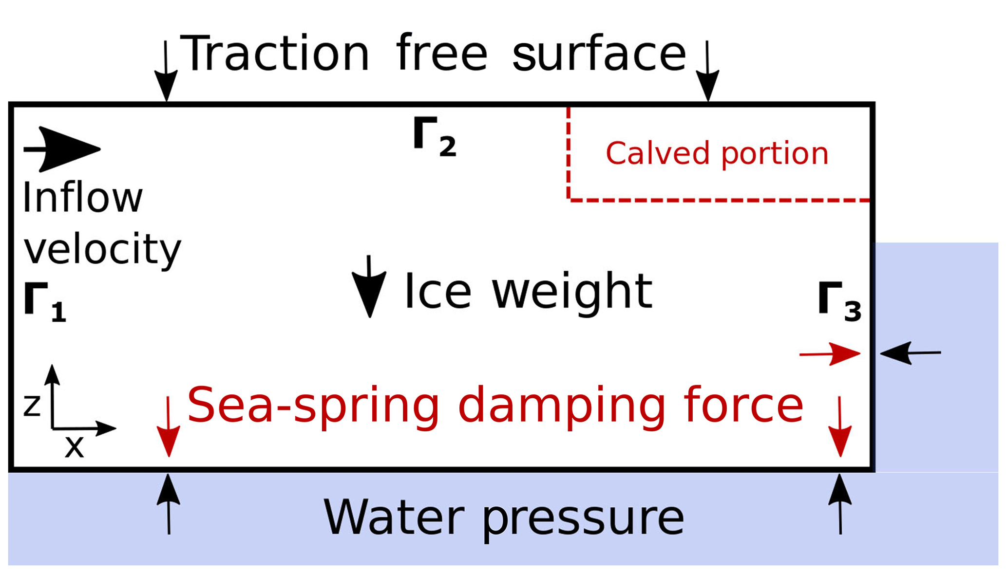
Figure 1A diagram showing the boundary conditions of an idealized floating ice shelf. The ice–ocean interface is subject to two normal stresses – the depth-dependent water pressure and the numerical damping force for stabilization to hydrostatic equilibrium. The dashed red line illustrates an iceberg that breaks off from the top of the calving front (exaggerated), reducing the freeboard and instantaneously perturbing the ice shelf from hydrostatic equilibrium.
2.2 Boundary conditions
To illustrate an example where the Stokes flow problem rapidly departs from hydrostatic equilibrium, we consider a two-dimensional floating ice shelf (Fig. 1). Along the inflow portion of the domain (Γ1), shear traction vanishes and we specify the normal component of the velocity , where u1 is a constant and is the normal vector along Γ1. At the ice–atmosphere boundary (Γ2) we assume the surface is traction free. At the boundary between ice and ocean (Γ3) the shear traction along the ice interface vanishes, and continuity of normal traction along the ice–ocean interface can be written as , where b(x,t) is the position of the ice–ocean interface.
Problems arise with this form if the glacier is not exactly in hydrostatic equilibrium because buoyancy forces along the ice–ocean interface cannot be balanced by internal stresses. In this case, there is no unique solution. In reality, of course, inertial effects are not negligible and the ice will quickly readjust to hydrostatic equilibrium as a consequence of buoyant uplift through the (nearly) inviscid ocean.
We can more appropriately specify the boundary condition for Stokes flow at the ice–ocean interface by writing it in the form
where Δz(x,t) is an a priori unknown isostatic adjustment that could potentially include a rigid body translation and, for a freely floating iceberg, rigid body rotation. Crucially, the rigid body motion must be determined as part of the solution to enable the local and global force balance to close.
The additional isostatic adjustment term Δz has a simple physical explanation: if normal stress was exactly hydrostatic, σnn=ρigH, where H is the ice shelf thickness. Equation (5) can then be solved for Δz to determine the position of the bottom interface needed for the forces to balance, which is exactly what is done in the shallow shelf approximation. The full Stokes approximation is more complex as internal stresses also contribute to the normal stress at the ice–ocean interface, but the location of the ice–ocean interface needs to be solved for as part of the solution to the problem, which we examine next.
2.3 Numerical stabilization of buoyant uplift
Different numerical methods use different techniques to estimate Δz in Eq. (5). For example, in Elmer/Ice, a popular package for modeling Stokes glacier flow, Durand et al. (2009) proposed an ingenious solution in which Δz is estimated based on a Taylor series of vertical position of the ice–ocean interface:
This Taylor series transforms the isostatic adjustment into a time-step-dependent Newtonian velocity damping:
Here, the velocity uz can include rigid body translation. The coefficient of the damping force in this approximation is proportional to the time step size Δt and vanishes in the limit of small Δt. We refer to the damping method given in Eq. (7) as the “sea-spring” method based on the nomenclature used in Elmer/Ice documentation.
We illustrate the time step dependence using a floating ice shelf as an example. In this case, global force balance is not guaranteed, leading to a formally ill-posed problem. However, the lack of a solution (which results in an exceptionally large velocity using the sea-spring stabilization) persists even when grounded ice is included in the domain because the velocity (and strain rate) solution can become unphysically sensitive to the position of the ice–ocean interface.

Figure 2L2 norm of (a) vertical velocity, (b) effective strain rate, (c) maximum shear stress, and (d) greatest principal stress immediately after the emulated calving event. The norm is calculated based on cell-averaged values. Solutions after a single time step are shown for sea-spring damping and sea-spring with Navier–Stokes (NS) for time step size ranging from 1 s to 30 years. The sea-spring with Navier–Stokes term gives physical solutions for all time steps but still shows variability with a time step consistent with the evolution of the system.
For our test, we implement an idealized rectangular ice shelf of thickness 400 m and length 10 km. This ice shelf is initialized to be in exact hydrostatic equilibrium. We set the inflow velocity for the upstream boundary condition to 4 km a−1. These thickness and velocity parameters are broadly consistent with observations for the last 10 km of Pine Island ice shelf (Rignot et al., 2017, 2011; Mouginot et al., 2012; Paden et al., 2010). The temperature-dependent constant in Glen's flow law is chosen to be 1.4×10⁸ Pa s1∕3, the value given by Cuffey and Paterson (2010) for −10 ∘C.
To emulate the occurrence of a calving event that would perturb the ice shelf from hydrostatic equilibrium, a rectangular section of length 50 m and thickness 20 m is removed from the upper calving front of the glacier (Fig. 1). This type of calving behavior has been proposed as the trigger of a larger calving mechanism related to buoyant stresses on the ice shelf (Wagner et al., 2014). The numerical effects we document are not unique to this style of calving, and this mechanism is only meant to illustrate the numerical issues.
The problem is implemented in FEniCS (Alnæs et al., 2015), an open-source finite element solver with a Python interface that has been previously used for Stokes glacier modeling (Ma et al., 2017; Ma and Bassis, 2019). The problem is solved using an arbitrary Lagrangian–Eulerian formulation using mixed Taylor–Hood elements with quadratic elements for velocity and linear elements for pressure. The open-source finite element mesh generator Gmsh is used to generate an unstructured mesh with uniform grid spacing of 10 m near the calved portion of the domain and grid spacing of 40 m elsewhere.
In Fig. 2, we show the L2 norm of vertical velocity, effective strain rate, maximum shear stress, and greatest principal stress immediately after the calving event, but computed using different values for Δt in Eq. (7). This shows the sensitivity of the vertical velocity, effective strain rate, maximum shear stress, and greatest principal stress to time step size when using the sea-spring boundary condition. In addition to the behavior of the L2 norm, we also examine the maximum value of the maximum shear stress and greatest principal stress (Fig. 3). Maximum values may be a better predictor of the effect of time step dependence on the results of Stokes calving models. Because calving models often assume that calving is likely if a stress threshold is exceeded (Ma et al., 2017), outliers in stress are more important than a stress averaged over the entire domain.
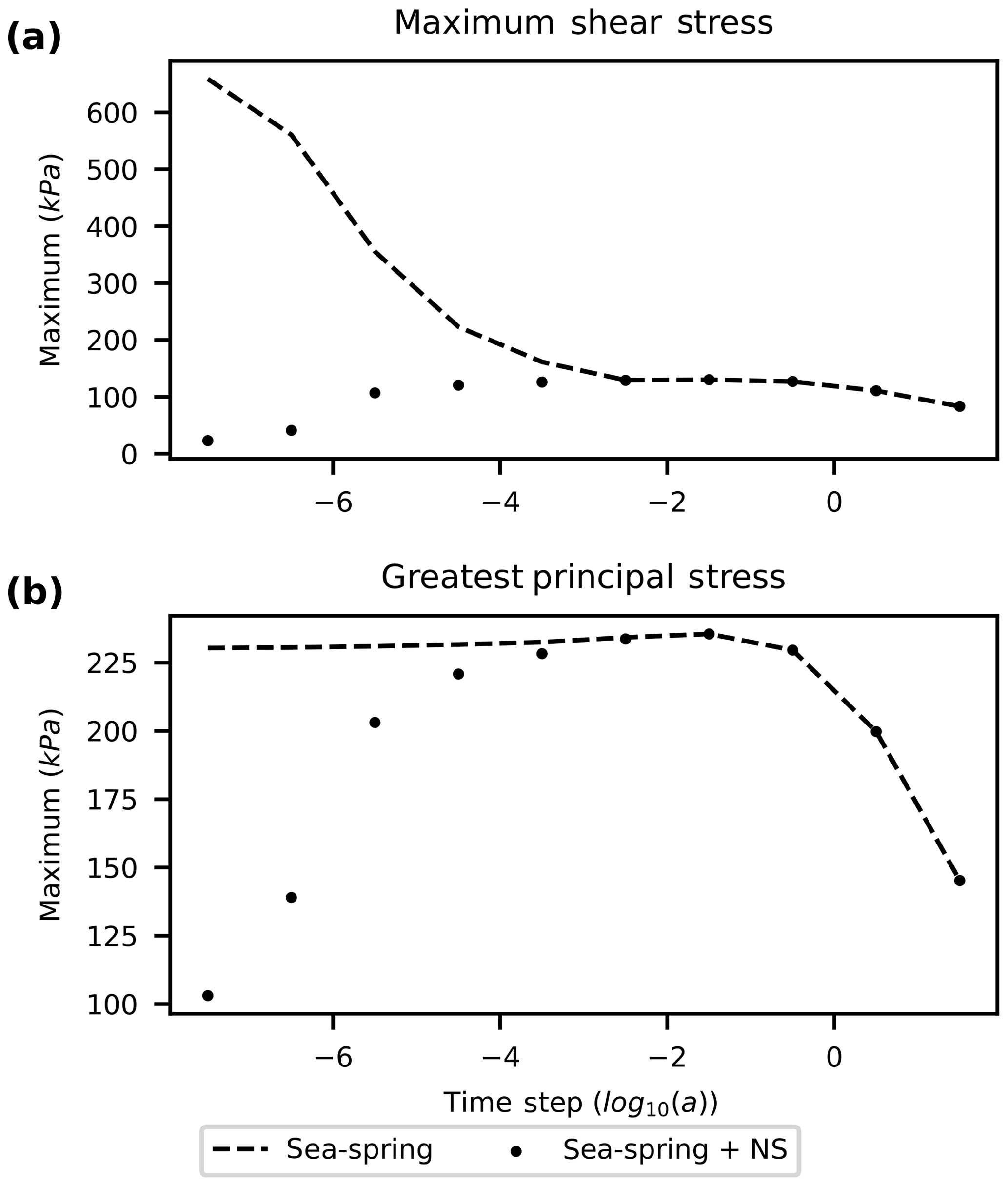
Figure 3Maximum (a) maximum shear stress and (b) greatest principal stress immediately after the emulated calving event. The maximum is calculated based on cell-averaged values. Solutions after a single time step are shown for sea-spring damping and sea-spring with Navier–Stokes (NS) for time step size ranging from 1 s to 30 years. Without corrections, maximum stress is overestimated in the Stokes model, which could lead to overestimation of glacier retreat due to calving.
The velocity solution is unphysical because the neglected acceleration term is not actually small relative to the other terms in Eq. (1). This is because large velocities associated with hydrostatic adjustment rapidly change on timescales that are short compared to the internal deformation of the ice. It may be possible to separate a rigid body translation and rotation that satisfies global force and torque balance from the internal deformation, but this quickly becomes cumbersome and impractical when we include the potential for ice to break: global force and torque balance would have to be maintained on each intact portion of ice. Instead, we reintroduce the acceleration term directly to the Stokes equation and show that this regularizes the solution for small time steps. We use a simple first-order backwards differentiation scheme in a Lagrangian reference frame:
where ui and ui−1 denote the velocity of Lagrangian fluid parcels at the current time step and the velocity at the previous time step, respectively. In the example considered here, the fixed horizontal velocity at the upstream boundary does not permit rigid body rotation and Eq. (8) remains a valid approximation even in an Eulerian coordinate system. As an initial condition on velocity, we assume a uniform velocity field of 4 km a−1 (equal to the inflow velocity) in the horizontal direction and zero in the vertical direction. The choice of zero initial velocity in the vertical direction is consistent with the idea that the ice shelf has instantaneously been perturbed from hydrostatic equilibrium.
Restoring the inertial term effectively introduces a Newtonian damping term on the entire body of the glacier where the damping coefficient is . Computational difficulty is not impacted by reintroducing the acceleration term in this way because the term is linear with respect to velocity. However, unless a fully implicit scheme was implemented, the solution becomes inaccurate (and unstable) for long time steps. Therefore, we propose to use both damping terms so that the system of equations is numerically accurate for all time step sizes.
When we include both damping terms, vertical velocity, effective strain rate, maximum shear stress, and greatest principal stress maintain physical values for both small and large time steps (Fig. 2). At small time steps the acceleration term dominates and the sea-spring with Navier–Stokes solution departs from the sea-spring solution. In this limit, the (nearly) rigid body isostatic adjustment of the ice shelf dominates the solution. By contrast, for large time steps, the sea-spring damping dominates and the two methods overlap. At intermediate time steps, both damping terms contribute as the solution transitions from the regime dominated by inertial effects to one where inertial effects are small. It is crucial to note that although the sea-spring with Navier–Stokes solution retains time step dependence for small time steps, the time step dependence now results from the physical evolution of the system: the solution resolves the acceleration and deceleration of the glacier as it bobs up and down in the ocean and approaches a steady state.
Although the sea-spring solution shows a smaller L2 norm of greatest principal stress than the sea-spring with Navier–Stokes solution, this is due to large negative compressive stresses associated with being outside of hydrostatic equilibrium. If we instead examine the maximum of the stress fields, the sea-spring solution shows larger values for both maximum shear stress and greatest principal stress (Fig. 3). This is particularly evident for the maximum shear stress, which is overestimated by an order of magnitude at the shortest time step tested. In the footloose calving mechanism, when a portion of the upper calving front is removed, the front of the ice shelf becomes buoyant and produces increased shear stress upstream on the ice shelf (Wagner et al., 2014). This overprediction of stresses could cause a calving model to predict unphysical calving events due to numerical inaccuracies.
Our study shows that using a common numerical stabilization method of the ice–ocean boundary in Stokes glacier modeling, there is an explicit time step dependence of the solution that is unphysical for small time steps when the domain rapidly departs from hydrostatic equilibrium. For model applications where changes in the domain are only due to viscous flow, the time step dependence is not problematic as long as domains are (nearly) in hydrostatic equilibrium at the start of simulation. However, for applications where rapid changes to the model domain occur, such as when calving rules are implemented, sudden departure from hydrostatic equilibrium is not only possible but expected. In these cases, time step dependence of the solution will appear. This can contaminate solutions of the stress after calving, potentially leading to a cascade of calving events and an overestimate of calving flux if numerical artifacts are not addressed. However, the time step dependence can be easily cured with little computational cost by reintroducing the acceleration term to the Stokes flow approximation. The acceleration term regularizes the solution for small time step sizes and provides consistent solutions for all time steps.
Code to run the tests in this paper is available at https://doi.org/10.5281/zenodo.4034850 (Berg, 2020).
BB identified the numerical issue with guidance from JB. BB and JB developed the proposed solution to the numerical issue. BB prepared the manuscript with contributions from JB.
The authors declare that they have no conflict of interest.
This work is from the DOMINOS project, a component of the International Thwaites Glacier Collaboration (ITGC). Logistics were provided by NSF's U.S. Antarctic Program and NERC's British Antarctic Survey (ITGC contribution no. ITGC:010).
This research has been supported by the National Science Foundation, Office of Polar Programs (grant no. 1738896) and the Natural Environment Research Council (grant no. NE/S006605/1).
This paper was edited by Valentina Radic and reviewed by Christian Schoof and one anonymous referee.
Alnæs, M., Blechta, J., Hake, J., Johansson, A., Kehlet, B., Logg, A., Richardson, C., Ring, J., Rognes, M. E., and Wells, G. N.: The FEniCS Project Version 1.5, Archive of Numerical Software, 3, 9–23, https://doi.org/10.11588/ans.2015.100.20553, 2015. a
Benn, D. I., Åström, J., Zwinger, T., Todd, J., Nick, F. M., Cook, S., Hulton, N. R., and Luckman, A.: Melt-under-cutting and buoyancy-driven calving from tidewater glaciers: new insights from discrete element and continuum model simulations, J. Glaciol., 63, 691–702, https://doi.org/10.1017/jog.2017.41, 2017. a
Berg, B.: brberg/stokes-time-step-dependence: Initial Release (Version v1.0.0), 17 September 2020, Zenodo, https://doi.org/10.5281/zenodo.4034850, 2020. a
Cuffey, K. M. and Paterson, W. S. B.: The physics of glaciers, Elsevier, Butterworth-Heineman, Burlington, MA, 4 edn., 2010. a
Durand, G., Gagliardini, O., de Fleurian, B., Zwinger, T., and Le Meur, E.: Marine ice sheet dynamics: Hysteresis and neutral equilibrium, J. Geophys. Res-Earth., 114, F03009, https://doi.org/10.1029/2008JF001170, 2009. a
Gagliardini, O., Zwinger, T., Gillet-Chaulet, F., Durand, G., Favier, L., de Fleurian, B., Greve, R., Malinen, M., Martín, C., Råback, P., Ruokolainen, J., Sacchettini, M., Schäfer, M., Seddik, H., and Thies, J.: Capabilities and performance of Elmer/Ice, a new-generation ice sheet model, Geosci. Model Dev., 6, 1299–1318, https://doi.org/10.5194/gmd-6-1299-2013, 2013. a
Greve, R. and Blatter, H.: Dynamics of ice sheets and glaciers, Springer, Berlin, 2009. a
Ma, Y. and Bassis, J. N.: The Effect of Submarine Melting on Calving From Marine Terminating Glaciers, J. Geophys. Res-Earth., 124, 334–346, https://doi.org/10.1029/2018JF004820, 2019. a, b, c
Ma, Y., Tripathy, C. S., and Bassis, J. N.: Bounds on the calving cliff height of marine terminating glaciers, Geophys. Res. Lett., 44, 1369–1375, https://doi.org/10.1002/2016GL071560, 2017. a, b, c, d
Mouginot, J., Scheuchl, B., and Rignot, E.: Mapping of ice motion in Antarctica using synthetic-aperture radar data, Remote Sens.-Basel, 4, 2753–2767, https://doi.org/10.3390/rs4092753, 2012. a
Nick, F. M., Van der Veen, C. J., Vieli, A., and Benn, D. I.: A physically based calving model applied to marine outlet glaciers and implications for the glacier dynamics, J. Glaciol., 56, 781–794, 2010. a
Paden, J., Li, J., Leuschen, C., Rodriguez-Morales, F., and Hale, R.: IceBridge MCoRDS L2 Ice Thickness, Version 1, Boulder, Colorado USA, NASA National Snow and Ice Data Center Distributed Active Archive Center, 2010, updated 2018. a
Rignot, E., Mouginot, J., and Scheuchl, B.: Ice Flow of the Antarctic Ice Sheet, Science, 333, 1427–1430, https://doi.org/10.1126/science.1208336, 2011. a
Rignot, E., Mouginot, J., and Scheuchl, B.: MEaSUREs InSAR-Based Antarctica Ice Velocity Map, Version 2, Boulder, Colorado USA, NASA National Snow and Ice Data Center Distributed Active Archive Center, 2017. a
Todd, J. and Christoffersen, P.: Are seasonal calving dynamics forced by buttressing from ice mélange or undercutting by melting? Outcomes from full-Stokes simulations of Store Glacier, West Greenland, The Cryosphere, 8, 2353–2365, https://doi.org/10.5194/tc-8-2353-2014, 2014. a, b, c
Todd, J., Christoffersen, P., Zwinger, T., Råback, P., Chauché, N., Benn, D., Luckman, A., Ryan, J., Toberg, N., Slater, D., and Hubbard, A.: A Full-Stokes 3-D Calving Model Applied to a Large Greenlandic Glacier, J. Geophys. Res-Earth., 123, 410–432, https://doi.org/10.1002/2017JF004349, 2018. a
Wagner, T. J. W., Wadhams, P., Bates, R., Elosegui, P., Stern, A., Vella, D., Abrahamsen, E. P., Crawford, A., and Nicholls, K. W.: The “footloose” mechanism: Iceberg decay from hydrostatic stresses, Geophys. Res. Lett., 41, 5522–5529, https://doi.org/10.1002/2014GL060832, 2014. a, b, c
Yu, H., Rignot, E., Morlighem, M., and Seroussi, H.: Iceberg calving of Thwaites Glacier, West Antarctica: full-Stokes modeling combined with linear elastic fracture mechanics, The Cryosphere, 11, 1283–1296, https://doi.org/10.5194/tc-11-1283-2017, 2017. a