An analysis of instabilities and limit cycles in glacier-dammed reservoirs

Glacier lake outburst floods are common glacial hazards around the world. How big such floods can become (either in terms of peak discharge or in terms of total volume released) depends on how they are initiated: what causes the runaway enlargement of a subglacial or other conduit to start the flood, and how big can the lake get before that point is reached? Here we investigate how the spontaneous channelization of a linked-cavity drainage system can control the onset of floods. In agreement with previous work, we show that floods only occur in a band of water throughput rates in which steady reservoir drainage is unstable, and we identify stabilizing mechanisms that allow steady drainage of an ice-dammed reservoir. We also show how stable limit cycle solutions emerge from the instability and identify parameter regimes in which the resulting floods cause flotation of the ice dam. These floods are likely to be initiated by flotation rather than the unstable enlargement of a distributed drainage system.

1 Introduction

Glacier lake outburst floods or “jökulhlaups” are a glacial hazard in many parts of the world (e.g. Björnsson, 1988; Clague et al., 2012). In addition, they provide a window into subglacial drainage systems: most outburst floods involve the opening and closing of a subglacial conduit, driven by melting of its walls through heat dissipation in the turbulent flow of water and by viscous creep closure of the ice. In the early stages of the outburst flood, wall melting dominates through a positive feedback in which conduit enlargement leads to faster water flow and therefore more dissipation of heat. Later in the flood, creep closure accelerates as the lake level drops, eventually causing the conduit to close again and terminating the flood. Alternatively, the flood can terminate because the lake has run dry. The conduit then becomes partially air filled and closes with minimal flow going through it.

While the mechanics of the main discharge phase of an outburst flood are relatively well understood (Nye, 1976; Clarke, 1982, 2003; Fowler and Ng, 1996; Ng, 1998; Fowler, 1999; Kingslake and Ng, 2013; Kingslake, 2013), the mechanisms that initiate the flood are still poorly understood, even though they dictate the level to which the lake is able to fill and therefore the magnitude and timing of the flood. In other words, the challenge is not to explain how a single flood progresses once started, but how it starts and, more to the point, what makes repeated floods occur cyclically, as a self-sustaining oscillation in the drainage system (Fowler, 1999; Kingslake, 2015). The main discharge phase of the flood is generally only part of a larger cycle, which also comprises a slow recharge phase in which outflow from the lake is small or absent altogether, and the transition between the recharge and discharge phases, where both lake inflow and outflow are of comparable magnitude.

One possibility for flood initiation is that the lake simply fills to the level at which the ice dam starts to float, and a sheet flow emerges between ice and bed that subsequently channelizes (Flowers et al., 2004). This may occur irregularly in some lakes such as Grímsvötn due to exceptionally large inflow rates to the lake, for instance during volcanic eruptions, or as part of a repeating flood cycle in others (Bigelow et al., 2020). Some lakes are however known to initiate outburst floods before they reach that flotation level.

Motivated by the subglacial lake at Grímsvötn in Iceland, Ng (1998) and Fowler (1999) consider how outburst floods are initiated in a drainage system that consists of a Röthlisberger (R) channel (Röthlisberger, 1972). In the simplest version of their model, where the channel is fed purely by the lake, they find that the amplitude of floods grows from cycle to cycle and that water pressures exceeding ice overburden are eventually reached, meaning that floods should start through the flotation of the ice dam after a few cycles. At the heart of this behaviour is the fact that the R channel can shrink to progressively smaller sizes between successive floods, making it harder to reinitiate drainage.

Grímsvötn typically starts its flood when water levels are below flotation (Björnsson, 1988), without successive floods growing in amplitude, except when the flood results from a large increase in water input due to volcanic activity (Gudmundsson et al., 1997). To explain this behaviour, Fowler (1999) considers the effect of a water supply along the length of the R channel on its evolution. Such a water supply can maintain a minimum channel size even between outburst floods, with flow of water being directed partly into the lake and partly down-glacier to the margin, provided the glacier has a geometrical “seal”. As the lake fills, the flow divide inside the channel migrates towards the lake, and the flood begins when the divide reaches the edge of the lake.

While this mechanism successfully explains how limit cycles (stable, periodic oscillations in lake level) can emerge in the model, it also predicts that no water can leave the lake between floods. Tracer experiments conducted at Salmon Glacier in Canada (Fisher, 1973) demonstrate that lakes can leak continuously throughout their recharge phase. Summit Lake, dammed by the Salmon Glacier, also has a history of flood initiation at lake levels below the flotation level (Post and Mayo, 1971). At Gornersee in Switzerland, observations of water lake levels and inferences of lake water balance based on meteorological measurements over two consecutive years also suggest leakage and flood initiation below flotation level during one year and flood initiation at or above flotation level during the previous year, potentially in the absence of any pre-flood leakage (Huss et al., 2007). Observations at Hidden Creek Lake (Anderson et al., 2003) by contrast suggest no leakage prior to flood initiation, though that conclusion is again based on water balance estimates rather than direct tracer experiments.

In this paper, we consider an alternative mechanism by which floods can initiate in a recurring fashion without the need for a sealed lake, but with continuous leakage throughout the flooding-and-refilling cycle. We show that a conduit that is able to switch spontaneously between the behaviour typical of an R channel and the behaviour of a linked-cavity system (Kessler and Anderson, 2004; Schoof, 2010; Hewitt et al., 2012; Hewitt, 2013; Werder et al., 2013) can sustain limit cycles without leading to flotation of the glacier at flood initiation, and without requiring the flow-divide migration appealed to in Fowler (1999). Note that many elements of the model studied here were included in the earlier study of outburst flooding by Kessler and Anderson (2004), who were able to replicate leakage from a glacier-dammed reservoir before the onset of the outburst flood but did not attempt to reproduce recurring floods. It is unclear if their model would have been able to do so since, in common with the model due to Fowler (1999), the main trunk of their drainage system was set up as a pure R channel.

The behaviour studied in the present paper was first documented in a model by Schoof et al. (2014). In this paper, we approach the problem from a more theoretical perspective, focusing on the following: first, we delineate when a “lake” or other storage reservoir can be drained steadily, identify conditions under which steady drainage becomes unstable, and identify how that instability leads to a limit cycle. Next, we investigate how the amplitude and period of floods depends on reservoir size and inflow rate. As a corollary, we determine at which point (in parameter space) the model predicts that flotation does occur and a different flood initiation mechanism is likely to take over. In closing, we also briefly comment on the difference in flood dynamics caused by distributing water storage along the flow path rather than having a single water reservoir (Schoof et al., 2014). We outline how the classical runaway melt mechanism for outburst floods first described by Nye (1976) can be replaced as a mechanism for self-sustaining water pressure oscillations by a spatial phase shift between conduit size and water pressure along the flow path.

The original motivation for the work in Schoof et al. (2014) was to demonstrate that behaviour akin to outburst floods can occur in systems with limited or even distributed water storage, manifesting itself in the form of unforced water pressure oscillations. Such limited storage could in principle result from moulins or any other vertical shaft that can fill progressively with water as water pressure rises. Viewed from that alternative perspective, the present paper analyses a drainage model that has become widely adopted in the study of subglacial hydrology (Werder et al., 2013). We identify instabilities that spontaneously lead to self-sustained oscillations, describing the mechanisms behind them and delineating the regions in parameter space where they occur. This is likely to be useful in diagnosing the behaviour of such models, regardless of their specific application to large outburst floods emanating from easily identifiable glacier lakes.

We use a hierarchy of model versions, employing both a spatially extended, one-dimensional drainage system model and a “lumped”, box-type model that provides additional physical insight, as well as being the appropriate limit of the spatially extended model in the case of a long flow path. The paper is laid out as follows: in Sect. 2, we develop the spatially extended and lumped models. In Sect. 3.1 and 3.2, we identify instabilities in the lumped model. The evolution of that instability at finite amplitude is investigated in detail in Sect. 3.3 and 3.4, where we show that stable limit cycles emerge in the lumped model. In Sect. 4, we show that the lumped model replicates the behaviour of the spatially extended behaviour well in the classical parameter regime that corresponds to the drainage of large glacier-dammed lakes. We also show that the extended model is unstable in more exotic parameter regimes, where the lumped model is not, and investigate the resulting dynamics. These results are summarized in Sect. 5.1, and we briefly touch on the dynamics of systems with distributed water storage in Sect. 5.2, relegating detail to the Supplement.

2 Model

2.1 A continuum model for outburst floods

We use the one-dimensional continuum model for drainage through a single conduit stated in Schoof et al. (2014), building on similar models used elsewhere (e.g. Ng, 1998; Hewitt and Fowler, 2008; Schuler and Fischer, 2009; Schoof, 2010; Hewitt et al., 2012). Note that we use the term “conduit” here to refer to a generic drainage element that can evolve dynamically to behave as an R channel, in which dissipation and creep closure are the dominant mechanisms by which channel size changes, or as a cavity, in which opening due to sliding over bedrock and creep closure are dominant (Kessler and Anderson, 2004; Schoof, 2010).

Denoting conduit cross section by S(x,t), effective pressure by N(x,t) and discharge by q(x,t), where x is downstream distance and t is time, we put

$$\begin{array}{}\text{(1a)}& {\displaystyle \frac{\partial S}{\partial t}}& {\displaystyle }=c_{\mathrm{1}}\stackrel{\mathrm{̃}}{q}\mathrm{\Psi }+v_{\mathrm{o}}\left(S\right)-v_{\mathrm{c}}(S,N),\text{(1b)}& {\displaystyle \frac{\partial \stackrel{\mathrm{̃}}{q}}{\partial x}}& {\displaystyle }=\mathrm{0},\text{(1c)}& {\displaystyle }\stackrel{\mathrm{̃}}{q}& {\displaystyle }=q(S,\mathrm{\Psi }),\text{(1d)}& {\displaystyle }\mathrm{\Psi }& {\displaystyle }={\mathrm{\Psi }}_{\mathrm{0}}+{\displaystyle \frac{\partial N}{\partial x}},\end{array}$$

on $\mathrm{0}<x<L$, subject to boundary conditions

$$\begin{array}{}\text{(1e)}& {\displaystyle }-V_p\left(N\right){\displaystyle \frac{\partial N}{\partial t}}& {\displaystyle }=q_{\mathrm{in}}-\stackrel{\mathrm{̃}}{q}& {\displaystyle }\text{at }x& {\displaystyle }=\mathrm{0},\text{(1f)}& {\displaystyle }N& {\displaystyle }=\mathrm{0}& {\displaystyle }\text{at }x& {\displaystyle }=L,\end{array}$$

where L is the length of the flow path, and we assume the closures

$$\begin{array}{}\text{(1g)}& \begin{array}{rl}& v_{\mathrm{o}}\left(S\right)=u_{\mathrm{b}}{h}_{\mathrm{r}}(\mathrm{1}-S/S_{\mathrm{0}}),v_{\mathrm{c}}(S,N)=c_{\mathrm{2}}S|N{|}^{n-\mathrm{1}}N,\\ & q(S,\mathrm{\Psi })=c_{\mathrm{3}}{S}^{\mathit{\alpha }}|\mathrm{\Psi }{|}^{-\mathrm{1}/\mathrm{2}}\mathrm{\Psi }.\end{array}\end{array}$$

Here c₁, c₂, c₃, n, α, u_b, h_r and S₀ are positive constants described in further detail below, with α>1, while q_in is also prescribed as a function of time and V_p>0 is a function of N. Ψ₀ is a geometrically determined background hydraulic gradient, given in terms of ice surface elevation s(x) and bed elevation b(x) through

$$\begin{array}{}\text{(1h)}& {\mathrm{\Psi }}_{\mathrm{0}}=-{\mathit{\rho }}_{\mathrm{i}}g{\displaystyle \frac{\partial s}{\partial x}}-({\mathit{\rho }}_{\mathrm{w}}-{\mathit{\rho }}_{\mathrm{i}})g{\displaystyle \frac{\partial b}{\partial x}}.\end{array}$$

Here ρ_w and ρ_i are the densities of ice and water, respectively, and g is acceleration due to gravity. Note that effective pressure N is linked to water pressures p_w, which is the primary observable in the field, through

$$\begin{array}{}\text{(1i)}& N=p_{\mathrm{i}}-p_{\mathrm{w}},\end{array}$$

where p_i is overburden (or more precisely, normal stress in the ice at the bed, averaged over a length scale much larger than that occupied by the conduit). Typically (including in Eq. 1h), p_i is assumed to be cryostatic, equal to ρ_ig(s−b).

Physically, the model represents a conduit whose size evolves due to a combination of dissipation-driven wall melting at a rate c₁qΨ, opening due to ice sliding over bed roughness at rate $u_{\mathrm{b}}{h}_{\mathrm{r}}(\mathrm{1}-S/S_{\mathrm{0}})$ and creep closure at rate c₂SNⁿ, with discharge in the conduit given by a Darcy–Weisbach or Manning friction law as $c_{\mathrm{3}}{S}^{\mathit{\alpha }}|\mathrm{\Psi }{|}^{-\mathrm{1}/\mathrm{2}}\mathrm{\Psi }$ through Eq. (1g). u_b is sliding velocity, h_r is bed roughness and S₀ is a cut-off cavity size at which bed roughness is drowned out (Schoof et al., 2012). S₀ is typically a regularizing parameter that prevents conduits from becoming excessively large in regions where effective pressures are low, such as near the glacier terminus, but has little effect on conduit sizes along most of the flow path; this corresponds to the limit of large S₀. Equation (1a) also ignores the effect of water pressure on the melting point, which affects the fraction of the dissipated heat available for melting of the conduit walls (Röthlisberger, 1972; Werder, 2016). We have also neglected the effect of water storage in the conduits and of dissipation-driven melting in the mass balance relation (1b); the reason for this is that a simple scaling exercise shows that these terms are invariably small for a terrestrial glacial system (Supplement Sect. S2.2).

Figure 1 Geometry of the problem: the conduit runs along the ice–bed interface.

Vanishing effective pressure at the end of the flow path x=L simply reflects the assumption that overburden and water pressure vanish simultaneously (where we have neglected atmospheric pressure as a gauge throughout). A computationally preferable assumption to N=0 may be to assume that there is an ice cliff at the glacier terminus, so that vanishing water pressure still corresponds to a finite N and the effect of dissipation-driven opening does not have to be offset by an unrealistic closing of the conduit through the sliding term, which becomes negative when S>S₀; our results are however not sensitive to this assumption.

The upstream boundary condition at x=0 reflects water storage in a reservoir at the head of the conduit: Eq. (1e) represents conservation of mass in the reservoir, with inflow rate q_in, with outflow at rate q(0,t) through the conduit modelled by Eqs. (1a)–(1d) and with water storage V in the reservoir a function of effective pressure at x=0 such that $\mathrm{d}V/\mathrm{d}N=-V_p$ (see e.g. Clarke, 2003). Note that we deliberately use “reservoir” rather than “lake” here since we will be interested not only in large lakes, but also in more modest-sized reservoirs as in Schoof et al. (2014). We will treat V_p and q_in as constants in most of what follows, although realistic lake shapes may argue for particular forms of the function V_p(N) (Clarke, 2003).

For simplicity, we have neglected the possibility of a partially air filled conduit and the effects of overpressurization, where effective pressure becomes negative (Schoof et al., 2012; Hewitt et al., 2012). Overpressurization is particularly relevant to the initiation mechanism for subglacial floods where unstable enlargement of the conduit is not fast enough for the flood to occur before the lake reaches N=0 and overfills. A partially air filled conduit may form by contrast at the upstream end of the flood path if the lake fully drains at the end of the outburst floods, and it could form more permanently at the downstream end as shown in Hewitt et al. (2012). We defer consideration of both processes to future work.

There is an important simplification we have made, irrespective of the particular choice of V_p: our model effectively imposes an ice cliff at the conduit inlet x=0, with the cliff height typically above the flotation thickness. This ensures that N(0,t) can change over time without the upstream end of the conduit migrating. This contrasts with a glacier that partially floats on the lake, in which case the upstream end of the conduit is always at N=0. In that case, the upstream conduit end migrates as the lake fills or empties, and its location is related to lake volume (see Sect. S2.4 of the Supplement).

The assumption of an ice cliff, in addition, allows us to assume that Ψ₀>0 along the entire flow path, without a seal at a finite distance from the reservoir at which Ψ₀ changes sign (Fowler, 1999). With a seal, there is a finite region of negative Ψ₀ between reservoir and seal location, with water flow out of the reservoir possible only when local effective pressure gradients $\partial N/\partial x$ are large enough to overcome the effects of the seal to make the total hydraulic gradient Ψ positive in Eq. (1d). In the absence of a seal and without an ice cliff (so N=0 at the edge of the reservoir), normal stress at the glacier bed just outside of the reservoir would then be below the flotation pressure, and there would be nothing to dam the reservoir (see Sect. S2.4 of the Supplement).

The two situations (an ice cliff and a seal) can be reconciled in the sense that a seal very close to the edge of the reservoir corresponds to a short, steep ice surface slope rather than an actual cliff. This results in a large, negative Ψ₀ between reservoir and seal over a short distance, which can be balanced by an equally large $\partial N/\partial x$ over the same short distance, leading to a non-zero effective pressure at the seal itself, only a short distance from the lake.

Nevertheless, our simplifying assumption is relevant as the mechanism for initiating periodically recurring floods is fundamentally different from that in Fowler (1999): his model relies on a geometrical seal with negative Ψ₀ near the reservoir, changing sign at the seal location, and an englacial water supply to the conduit that dictates the gradient $\partial N/\partial x$ while the lake is filling. As described in the introduction, the onset of the outburst flood corresponds to the instant at which Ψ at the conduit inlet x=0 changes from negative to positive and allows water to flow out of the reservoir. This leads to runaway enlargement of the conduit through dissipation-driven melting.

By contrast, our model assumes that the reservoir always experiences some amount of leakage and requires no englacially supplied conduit: the water supply to the drainage system in our model is purely through the inflow term q_in into the reservoir. Leakage out of the reservoir is facilitated by the linked-cavity behaviour of the conduit between floods, associated with the cavity opening term v_o that keeps the conduit open even when flow rates are small. This is absent from the models in Fowler (1999) and Ng (1998). As the lake fills, these cavities enlarge because the effective pressure is reduced, and the conduit then grows through the same melt-driven conduit enlargement as in Fowler (1999) and Ng (1998), but the initiation of that enlargement differs.

2.2 A lumped model

The model (1) can be simplified if we assume that Ψ₀ not only does not change sign along the flow path but can be treated as a constant and if we assume that the effective pressure gradient $\partial N/\partial x$ along the flow path can be treated as negligible (see also Fowler, 1999; Ng, 2000, and Sect. S2.2 and S2.3 of the Supplement) or approximated by a simple divided difference.

Under these assumptions, we can relate the flux q along the flow path (which is independent of position by Eq. 1b) purely to the conduit size S and hydraulic gradient Ψ₀ at the head of the conduit, leading to a system of ordinary rather than partial differential equations:

$$\begin{array}{}\text{(2a)}& {\displaystyle }\dot{S}& {\displaystyle }=c_{\mathrm{1}}\stackrel{\mathrm{̃}}{q}\mathrm{\Psi }+v_{\mathrm{o}}\left(S\right)-v_{\mathrm{c}}(S,N),\text{(2b)}& {\displaystyle }-V_p\dot{N}& {\displaystyle }=q_{\mathrm{in}}-\stackrel{\mathrm{̃}}{q},\text{(2c)}& {\displaystyle }\stackrel{\mathrm{̃}}{q}& {\displaystyle }=q(S,\mathrm{\Psi }),\end{array}$$

where a dot signifies an ordinary derivative with respect to time, and we continue to assume the closure relations (1g); by the argument above, we then strictly speaking have to put Ψ=Ψ₀. We generalize this reduced model slightly to account qualitatively, if not quantitatively, for the effect of pressure gradients along the flow path by putting

$$\begin{array}{}\text{(2d)}& \mathrm{\Psi }={\mathrm{\Psi }}_{\mathrm{0}}-N/L,\end{array}$$

which corresponds to a crude divided difference approximation of the actual gradient $\partial N/\partial x$ by $\left[N\right(L,t)-N(\mathrm{0},t\left)\right]/L$.

In what follows, we proceed first with an analysis of the simpler, lumped model (2), to which we can bring to bear the theory of finite-dimensional dynamical systems (Strogatz, 1994; Wiggins, 2003), leading a number of semi-analytical results. Subsequently, we study the full, spatially extended model (1), for which we are limited to comparatively expensive numerical methods that we can guide by our analysis of the simpler, lumped model.

3 An analysis of the lumped model

3.1 Nye's jökulhlaup instability in the reduced model

Nye's (1976) original theory of jökulhlaups centres on the idea that steady flow in an R channel is unstable if there is a water reservoir that keeps water pressure approximately constant. This instability results in the runway growth of a channel, eventually allowing the reservoir to drain in an outburst flood. The assumption of a constant effective pressure is of course a simplification of the more complete model (2), based on the notion that the drainage of the lake is generally too slow to lead to changes in effective pressure that could stabilize the channel against growth.

The basis of this instability is relatively easy to capture mathematically. To set the scene, we present a simplified version first before tackling an analysis of the complete model (2). If we assume a classical R channel in the sense of Röthlisberger (1972) and Nye (1976) and therefore set the cavity opening term v_o to zero in Eq. (2a), and use the remaining relations in Eq. (1g), the conduit evolution Eq. (2a) becomes

$$\begin{array}{}\text{(3)}& \dot{S}=c_{\mathrm{1}}{c}_{\mathrm{3}}{S}^{\mathit{\alpha }}|\mathrm{\Psi }{|}^{\mathrm{3}/\mathrm{2}}-c_{\mathrm{2}}S|N{|}^{n-\mathrm{1}}N,\end{array}$$

with a steady-state conduit size $\overline{S}$ given by $c_{\mathrm{2}}\overline{S}|\overline{N}{|}^{n-\mathrm{1}}\overline{N}=c_{\mathrm{1}}{c}_{\mathrm{3}}{\overline{S}}^{\mathit{\alpha }}|\mathrm{\Psi }{|}^{\mathrm{3}/\mathrm{2}}$. At fixed effective pressure N, and hence at fixed Ψ, this steady state is unstable: an increase S^′ away from the steady-state size $\overline{S}$ will lead to a further growth in the conduit, as we have $(\overline{S}+S^{\prime }{)}^{\mathit{\alpha }}\approx {\overline{S}}^{\mathit{\alpha }}+\mathit{\alpha }{\overline{S}}^{\mathit{\alpha }-\mathrm{1}}{S}^{\prime }$ and so

$$\begin{array}{}\text{(4)}& \begin{array}{rl}{\dot{S}}^{\prime }\approx & c_{\mathrm{1}}{c}_{\mathrm{3}}\mathit{\alpha }{\overline{S}}^{\mathit{\alpha }-\mathrm{1}}{S}^{\prime }|\mathrm{\Psi }{|}^{\mathrm{3}/\mathrm{2}}-c_{\mathrm{2}}{S}^{\prime }|N{|}^{n-\mathrm{1}}N\\ =& c_{\mathrm{1}}{c}_{\mathrm{3}}(\mathit{\alpha }-\mathrm{1}){\overline{S}}^{\mathit{\alpha }-\mathrm{1}}|\mathrm{\Psi }{|}^{\mathrm{3}/\mathrm{2}}{S}^{\prime },\end{array}\end{array}$$

where, with α>1, the right-hand side is positive if S^′ is, signifying that S^′ will continue to grow in a positive feedback.

In more abstract terms, if Ψ and N are fixed, Eq. (2a) can be expected to lead to unstable growth of conduits away from an equilibrium state $\overline{S}$ if (see also pp. 5–6 of the Supplement to Schoof, 2010)

$$\begin{array}{}\text{(5)}& c_{\mathrm{1}}{\left.{\displaystyle \frac{\partial q}{\partial S}}\right|}_{S=\overline{S}}\mathrm{\Psi }+{\left.{\displaystyle \frac{\partial v_{\mathrm{o}}}{\partial S}}\right|}_{S=\overline{S}}-{\left.{\displaystyle \frac{\partial v_{\mathrm{c}}}{\partial S}}\right|}_{S=\overline{S}}>\mathrm{0}.\end{array}$$

This is also precisely the condition that defines a conduit as being channel-like in Schoof (2010), in the sense that two neighbouring conduits will compete for water with one eventually growing at the expense of the other if both are channel-like.

Key to the instability mechanism above was the notion that effective pressure N is kept constant as the conduit evolves, which is not actually the case: instead, the lake simply buffers changes in N from happening rapidly. Next, we investigate in more detail how water storage and the finite size L of the system control whether Nye's instability does occur in the reduced model of Sect. 2.2.

Note that v_o, v_c and q satisfy

$$\begin{array}{}\text{(6)}& {\displaystyle \frac{\partial v_{\mathrm{o}}}{\partial S}}\le \mathrm{0},{\displaystyle \frac{\partial v_{\mathrm{c}}}{\partial S}}>\mathrm{0},{\displaystyle \frac{\partial v_{\mathrm{c}}}{\partial N}}>\mathrm{0},{\displaystyle \frac{\partial q}{\partial S}}>\mathrm{0},{\displaystyle \frac{\partial q}{\partial \mathrm{\Psi }}}>\mathrm{0},\end{array}$$

with v_o(S)>0 bounded as S→0, $v_{\mathrm{c}}(S,\mathrm{0})=\mathrm{0}$ and $v_{\mathrm{c}}(\mathrm{0},N)=\mathrm{0}$; q also has the same sign as Ψ and satisfies $q(\mathrm{0},\mathrm{\Psi })=q(S,\mathrm{0})=\mathrm{0}$. These are the minimal assumptions we make on these functions, allowing us to generalize from the specific forms in Eq. (1g) in analysing Nye's instability.

The primary dependent variables in the model (2) are S and N. For constant water input q_in, the model admits a steady state $(\overline{S},\overline{N})$ given implicitly by

$$\begin{array}{}\text{(7a)}& {\displaystyle }{c}_{\mathrm{1}}q(\overline{S},\overline{\mathrm{\Psi }})\overline{\mathrm{\Psi }}+v_{\mathrm{o}}\left(\overline{S}\right)-v_{\mathrm{c}}(\overline{S},\overline{N})& {\displaystyle }=\mathrm{0},\text{(7b)}& {\displaystyle }q(\overline{S},\overline{\mathrm{\Psi }})& {\displaystyle }=q_{\mathrm{in}},\text{(7c)}& {\displaystyle }\overline{\mathrm{\Psi }}& {\displaystyle }={\mathrm{\Psi }}_{\mathrm{0}}-\overline{N}/L,\end{array}$$

where we assume positive lake inflow q_in>0. It can be shown (see Sect. S3 of the Supplement) that there is a unique steady-state solution with positive $\overline{N}$, $\overline{S}$ and $\overline{\mathrm{\Psi }}$. To establish whether the solution is stable, we can linearize around the steady state as

$$N=\overline{N}+N^{\prime }\exp \left(\mathit{\lambda }t\right),S=\overline{S}+S^{\prime }\exp \left(\mathit{\lambda }t\right).$$

This yields the following eigenvalue problem

$$\begin{array}{}\text{(8)}& \begin{array}{rl}& \left(\begin{array}{cc}{c}_{\mathrm{1}}{q}_S\overline{\mathrm{\Psi }}+v_{\mathrm{o},S}-v_{\mathrm{c},S}-\mathit{\lambda }& -c_{\mathrm{1}}(q_{\mathrm{\Psi }}\overline{\mathrm{\Psi }}+\overline{q})L^{-\mathrm{1}}-v_{\mathrm{c},N}\\ {\overline{V}}_p^{-\mathrm{1}}{q}_S& -{\overline{V}}_p^{-\mathrm{1}}{q}_{\mathrm{\Psi }}{L}^{-\mathrm{1}}-\mathit{\lambda }\end{array}\right)\\ & \left(\begin{array}{c}{S}^{\prime }\\ N^{\prime }\end{array}\right)=\mathrm{0},\end{array}\end{array}$$

where

$$q_S={\left.{\displaystyle \frac{\partial q}{\partial S}}\right|}_{S=\overline{S},\mathrm{\Psi }=\overline{\mathrm{\Psi }}},q_{\mathrm{\Psi }}={\left.{\displaystyle \frac{\partial q}{\partial \mathrm{\Psi }}}\right|}_{S=\overline{S},\mathrm{\Psi }=\overline{\mathrm{\Psi }}},v_{\mathrm{o},S}={\left.{\displaystyle \frac{\mathrm{d}{v}_{\mathrm{o}}}{\mathrm{d}S}}\right|}_{S=\overline{S}},$$

$$v_{\mathrm{c},S}={\left.{\displaystyle \frac{\partial v_{\mathrm{c}}}{\partial S}}\right|}_{S=\overline{S},N=\overline{N}},v_{\mathrm{c},N}={\left.{\displaystyle \frac{\partial v_{\mathrm{c}}}{\partial N}}\right|}_{S=\overline{S},N=\overline{N}},{\overline{V}}_p=V_p\left(\overline{N}\right).$$

Setting the determinant of the matrix on the left to zero, we obtain a quadratic with solution

$$\begin{array}{}\text{(9)}& \mathit{\lambda }={\displaystyle \frac{\mathrm{1}}{\mathrm{2}}}\left[a_{\mathrm{1}}\pm \sqrt{a_{\mathrm{1}}^{\mathrm{2}}-\mathrm{4}{a}_{\mathrm{2}}}\right],\end{array}$$

where

$$\begin{array}{}\text{(10a)}& {\displaystyle }{a}_{\mathrm{1}}=c_{\mathrm{1}}{q}_S\overline{\mathrm{\Psi }}+v_{\mathrm{o},S}-v_{\mathrm{c},S}-{\overline{V}}_p^{-\mathrm{1}}{q}_{\mathrm{\Psi }}{L}^{-\mathrm{1}},\text{(10b)}& {\displaystyle }\begin{array}{rl}{a}_{\mathrm{2}}=& {\overline{V}}_p^{-\mathrm{1}}\left[c_{\mathrm{1}}{q}_S\overline{q}{L}^{-\mathrm{1}}+q_S{v}_{\mathrm{c},N}\right.\\ & \left.+q_{\mathrm{\Psi }}{L}^{-\mathrm{1}}(v_{\mathrm{c},S}-v_{\mathrm{o},S})\right].\end{array}\end{array}$$

From our assumptions on the various functions involved, we see that a₂>0 (recall that $v_{\mathrm{o},S}\le \mathrm{0}$ from the inequality Eq. 6), while a₁ can be either sign. Since a₂>0, we have $a_{\mathrm{1}}^{\mathrm{2}}-\mathrm{4}{a}_{\mathrm{2}}<a_{\mathrm{1}}^{\mathrm{2}}$ and two possible types of solution: either (i) $a_{\mathrm{1}}^{\mathrm{2}}-\mathrm{4}{a}_{\mathrm{2}}>\mathrm{0}$, in which case we have two real roots, both of which have the same sign as a₁, or (ii) $a_{\mathrm{1}}^{\mathrm{2}}-\mathrm{4}{a}_{\mathrm{2}}<\mathrm{0}$, resulting in a complex conjugate pair of roots, both of which have real part a₁. In either case, we see that the system is linearly unstable if and only if a₁>0, or

$$\begin{array}{}\text{(11)}& \left(c_{\mathrm{1}}{q}_S\overline{\mathrm{\Psi }}+v_{\mathrm{o},S}-v_{\mathrm{c},S}\right)-{\overline{V}}_p^{-\mathrm{1}}{q}_{\mathrm{\Psi }}{L}^{-\mathrm{1}}>\mathrm{0}.\end{array}$$

We have deliberately written the left-hand side of Eq. (11) as the difference of two terms, a potentially destabilizing term $c_{\mathrm{1}}{q}_S\overline{\mathrm{\Psi }}+v_{\mathrm{o},S}-v_{\mathrm{c},S}$ and a stabilizing term $-{\overline{V}}_p^{-\mathrm{1}}{q}_{\mathrm{\Psi }}{L}^{-\mathrm{1}}$. The first term can be recognized as the growth rate sensitivity we previously identified as being at the heart of Nye's instability in Eq. (5), as well as an indicator of whether the steady-state conduit is channel-like in the terminology of Schoof (2010).

The second term in the relation (11) is a stabilizing term that is inversely related to storage capacity. Its physical origin is the following: the sensitivity of conduit growth to perturbations in conduit size may be positive, potentially leading to unstable conduit growth. However, growth of the conduit also allows water to drain out of the system, which will increase the effective pressure N. As the effective pressure is increased, the hydraulic gradient $\mathrm{\Psi }={\mathrm{\Psi }}_{\mathrm{0}}-N/L$ is reduced. This leads to less turbulent dissipation in the conduit as the conduit grows, and increased N further leads to faster creep closure of the conduit. Both of these will suppress further growth of the conduit. How strong this stabilizing effect is will depend on the storage capacity of the system and on the length L of the flow path: a large storage capacity ${\overline{V}}_p$ or a long flow path L leads to a reduced stabilizing effect. In practice, we are likely to see stabilization for small storage elements, such as moulins and individual crevasses.

3.2 Stability boundaries

We have established that Nye's instability will occur if the conduit is channel-like and water storage in the system is sufficiently large, as well as if the system length L is big enough. Note that, with the choices in Eq. (1g), the system is always unstable if v_o=0 (so the conduit is always a channel) and L=∞ (so effective pressure does not alter the hydraulic gradient). This is in agreement with Ng (1998).

We can go further and determine explicitly the regions of parameter space in which this stability occurs. While we present our results here in dimensional form, note that it is possible to reduce the spatially extended and lumped models (1) and (2) to a four-dimensional parameter space by non-dimensionalizing them (Sect. S2.2 and S2.3 of the Supplement). These parameters are dimensionless versions of the inflow rate q_in, storage capacity V_p, system length L and conduit cut-off size S₀. Recall that S₀ is intended to have minimal impact on conduit evolution away from the glacier margin, and we are therefore interested in the limit of large S₀. As a result, we restrict ourselves to the three-dimensional parameter space spanned by $(q_{\mathrm{in}},{\overline{V}}_p,L)$ and set S₀=∞ in the lumped model (2). The remaining fixed parameter values we have used are given in Table 1. The low value of Ψ₀ stated corresponds approximately to a 1:50 surface slope.

Table 1 Parameter values common to all calculations except those in Fig.  12, for which Ψ₀=1630 Pa m⁻¹ (corresponding to a much steeper 17:100 slope), $u_{\mathrm{b}}{h}_{\mathrm{r}}=\mathrm{1.05}\times {\mathrm{10}}^{-\mathrm{07}}$ m² s⁻¹ and L=5 km.

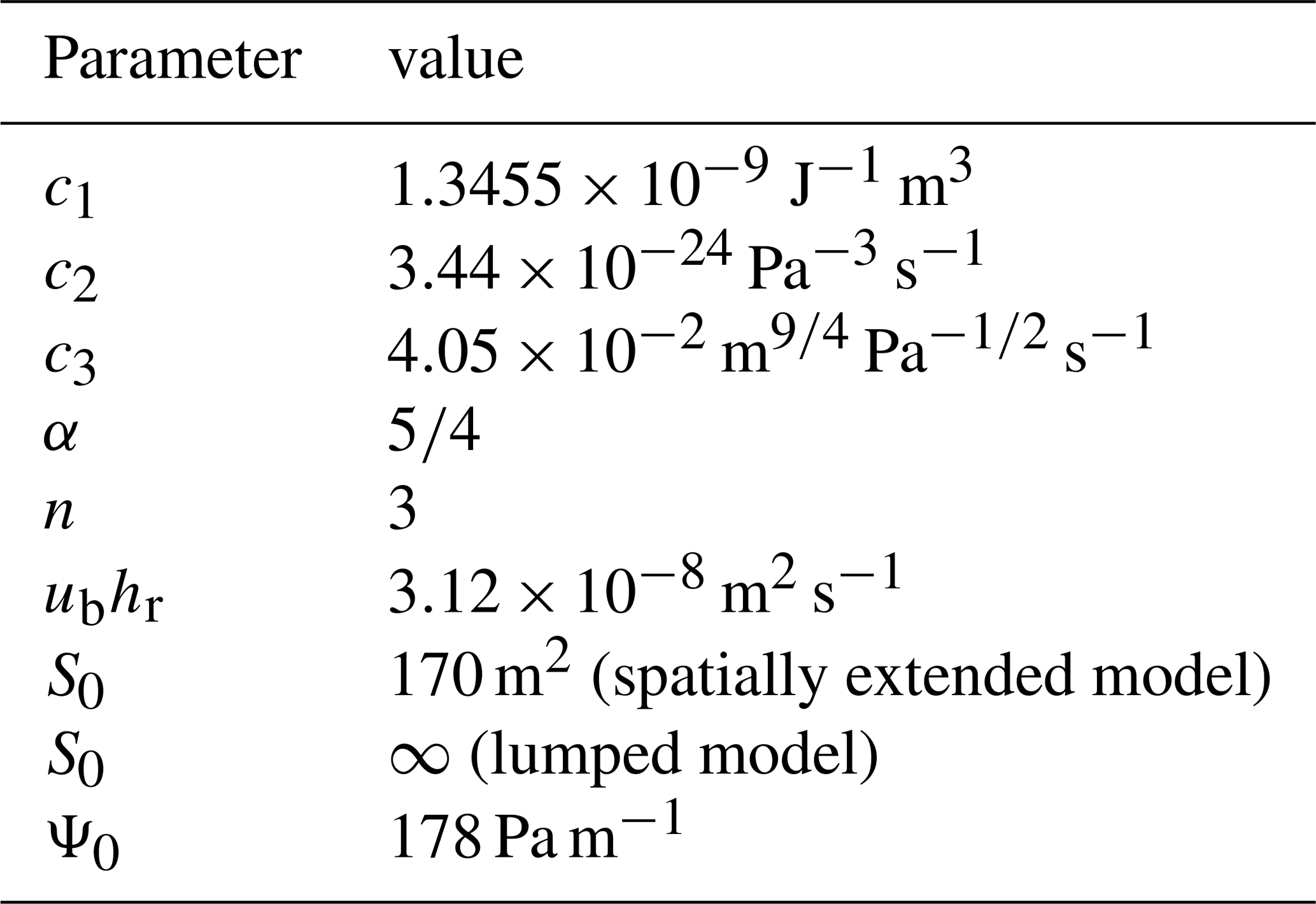
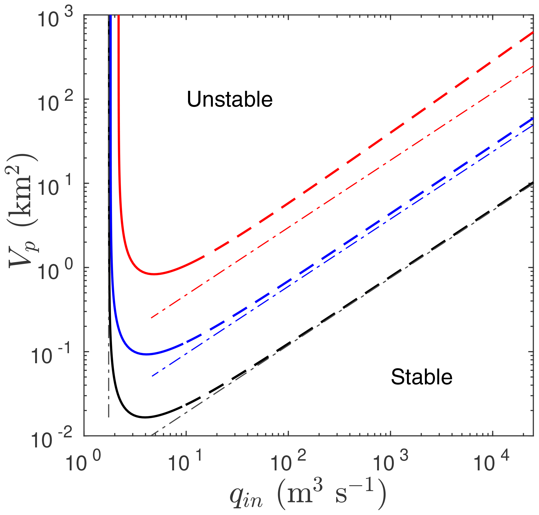
Figure 2 Stability boundaries for reservoir systems with the parameter values in Table 1 shown as solid/dashed curves. Note the logarithmic scales on the axes. The unstable region in parameter space is above the curves as shown. The curves correspond to different values of L: 10 km (red), 50 km (blue) and 250 km (black); the latter is not intended to be physically realistic but to reflect the limit of large L. The Hopf bifurcation at the stability boundary is supercritical where the curve is solid and subcritical where dashed (see Sect. 3.3). The dotted–dashed curves show the asymptotic stability boundaries given by Eqs. (12) and (13).

Figure 2 shows stability boundaries in the $(q_{\mathrm{in}},{\overline{V}}_p)$ plane for different values of L. These are the locations in parameter space where the real part of the growth rate λ in Eq. (9) is zero (see Sect. S3.2 of the Supplement for details); invariably, the eigenvalues λ then form a purely imaginary conjugate pair, and we have a so-called Hopf bifurcation (see Sect. 3.3 below). Note that ${\overline{V}}_p$ is displayed in units of square kilometres (km²), normalizing by ρ_wg; in other words, what is really plotted is ${\overline{V}}_p/\left({\mathit{\rho }}_{\mathrm{w}}g\right)$, the surface area of the lake (see Sect. 2). Similarly, we will plot N in units of metres (m) in subsequent figures, normalizing by ρ_wg: changes in N plotted then correspond directly to changes in water level in the lake.

In each case shown in Fig. 2, there is a region of instability above some critical value of ${\overline{V}}_p$, and for q_in in some intermediate range, where larger ${\overline{V}}_p$ is required and the unstable inflow range is shrunk for shorter flow path lengths L. This is consistent with theoretical results (Sect. S3.1 of the Supplement) showing that the system is always stable for either sufficiently small or sufficiently large q_in but can be unstable at intermediate inflow rates.

For large enough ${\overline{V}}_p$ and L, we can determine approximate analytical expressions for the stability boundaries. The lower critical value of q_in at which the drainage system first becomes unstable corresponds to the switch from a cavity-like to a channel-like conduit, and this occurs for large L at (see Schoof, 2010, and Sect. S3.1 of the Supplement)

$$\begin{array}{}\text{(12)}& q_{\mathrm{in}}={\displaystyle \frac{u_{\mathrm{b}}{h}_{\mathrm{r}}}{c_{\mathrm{1}}(\mathit{\alpha }-\mathrm{1}){\mathrm{\Psi }}_{\mathrm{0}}}}.\end{array}$$

Note that for finite h ${\overline{V}}_p$ and L, there is generally at least a small region of stability in which q_in is already large enough for the conduit to be channel-like (the space between the dotted–dashed vertical line and the solid curves in Fig. 2). This region exists because the first term in Eq. (11) is positive but not large enough to overcome the second, stabilizing term here.

The upper critical value of q_in at which the system stabilizes again can be similarly computed in the limit of large L by omitting the cavity opening term v_o and reducing the conduit evolution Eq. (2a) to a balance between the first (dissipation-driven melting) and third (creep-closure) terms on the right-hand side. This yields

$$\begin{array}{}\text{(13)}& {\overline{V}}_p\sim {\displaystyle \frac{q_{\mathrm{in}}^{\mathrm{1}/\mathit{\alpha }}}{\mathrm{2}(\mathit{\alpha }-\mathrm{1})c_{\mathrm{1}}{c}_{\mathrm{3}}^{\mathrm{1}/\mathit{\alpha }}{\mathrm{\Psi }}_{\mathrm{0}}^{(\mathrm{3}\mathit{\alpha }+\mathrm{2})/\left(\mathrm{2}\mathit{\alpha }\right)}L}}.\end{array}$$

These limiting forms are also shown in Fig. 2, where we see that they are most accurate for large L as expected.

3.3 Hopf bifurcations and limit cycles

The analysis above has been purely linear, identifying parameter regimes in which steady drainage is unstable. That linearization will eventually fail where unstable growth is predicted, and a non-linear model is needed to predict what the instability grows into. A key aspect of many outburst floods is that they are a recurring phenomenon. For the reduced model (2) with two dynamical degrees of freedom and steady forcing, such a recurrence must correspond to a stable periodic oscillation in the absence of time-dependent forcing (see also Kingslake, 2013, for time-dependent forcing that leads to chaotic solutions). As was underlined by Ng (1998) and Fowler (1999), the existence of such a limit cycle does not simply follow from the instability itself: we need to ensure that the evolution away from the steady state leads to bounded growth of the instability once it reaches a finite amplitude.

It is straightforward to demonstrate bounded growth in our model computationally. Figure 3 shows a sample calculation of a periodic solution, with the classical attributes of an outburst flood cycle: effective pressure slowly decreases during the interval between outburst floods, when conduit size is small. This is simply the lake refilling. As N approaches its minimum, the conduit size S starts to grow rapidly, initiating the outburst flood: effective pressure is no longer large enough to keep conduit size small, and enough water can flow to start enlarging the conduit in the runaway growth envisioned by Nye (1976). The lake then drains, rapidly increasing N. Once effective pressure gets large enough, creep closure becomes dominant, causing S to shrink again, and the cycle repeats. By contrast with Ng (1998) and Fowler (1999), key to this periodic behaviour is that the conduit cannot become arbitrarily small between floods, since it is kept open by ice flow over bed roughness.

In fact, S in our model actually starts to increase almost immediately after flood termination, as the refilling of the reservoir leads to decreasing effective pressure allowing the now cavity-like conduit to grow. As explained above, water flow through them will eventually lead to reinitiation of dissipation-driven melting and enlargement of the conduit. By contrast, once the amplitude of the floods has become large enough, conduit size in the pure channel model of Ng (1998) and Fowler (1999) keeps shrinking during the refilling phase until the effective pressure changes sign to negative, and this underpins the ever-increasing flood amplitudes in their model.

An alternative visualization of the physics involved is a phase plane, plotting S against N as the system evolves; a periodic solution then corresponds to a closed orbit. Figure 4 shows the phase plane equivalent of Fig. 3, with the dashed lines corresponding to nullclines (the curves on which either $\dot{S}=\mathrm{0}$ or $\dot{N}=\mathrm{0}$). During the refilling phase, the point (N(t),S(t)) closely follows the S nullcline, with S steadily increasing as explained above.

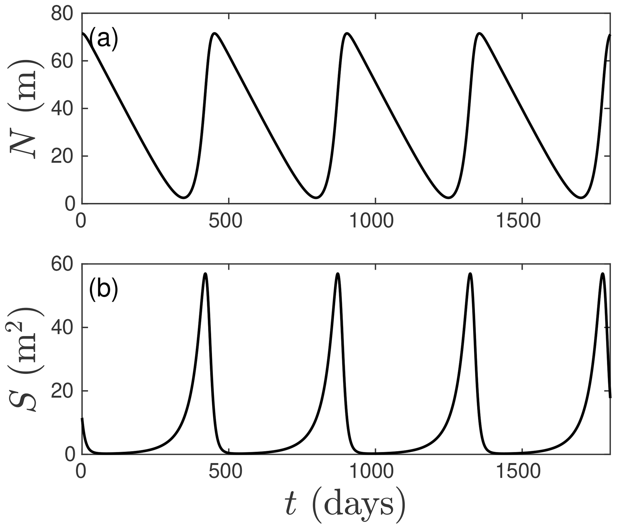
Figure 3 Periodic oscillations in the system (2) with parameter values as in Table 1, with V_p = 4 km², L = 50 km and q_in = 10.9 m³ s⁻¹.

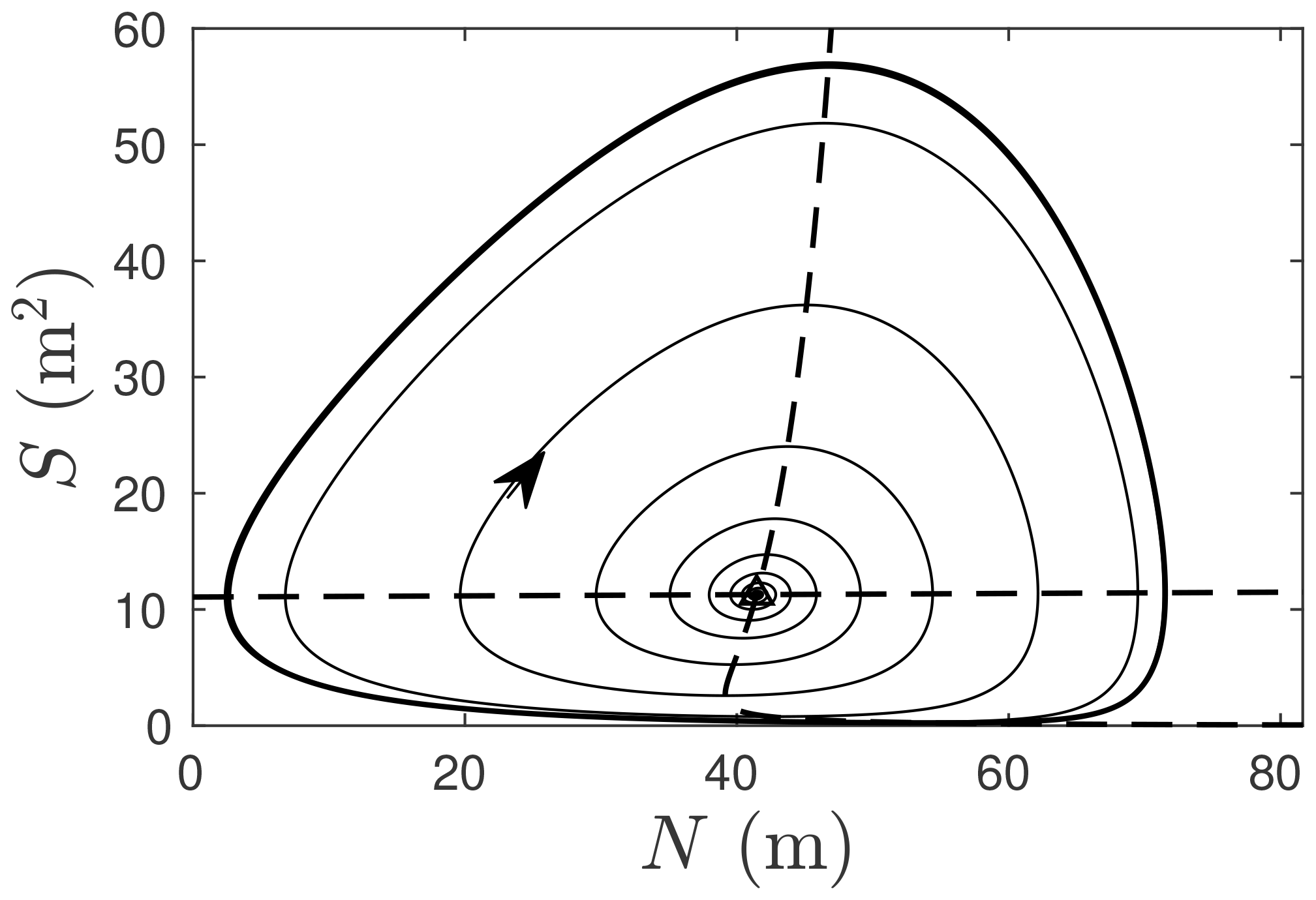
Figure 4 The periodic solution of Fig. 3 plotted in a phase plane. The thin curve represents a solution that approaches the limit cycle shown by the thick curve as indicated by the arrow. The instability of the steady-state solution (where the nullclines cross) is clearly visible, since evolution along the thin line is away from that steady state.

Figures 3 and 4 show only one example. It is possible to solve directly for such periodic solutions and trace how they change under parameter changes using an arc length continuation method (Sect. S3.4 of the Supplement), as well as to determine simultaneously whether the periodic solutions are stable: some periodic solutions are in fact never attained by forward integration of the model (2) because they are themselves unstable. Small perturbations will therefore cause the system to evolve away from them.

As in Sect. 3.2, we focus on how solutions change as the water input to the reservoir q_in is varied. Figure 5 shows how the amplitude of oscillations varies with water input for a fixed L=50 km and different storage capacity V_p (treated as independent of N here). In each panel, the coloured curve (black in Fig. 5e) shows the minimum and maximum value of N attained for a periodic solution at the corresponding value of q_in (i.e. the values of N where the corresponding orbit in the phase plane crosses the N nullcline). Solid portions of these coloured curves in Fig. 5 correspond to stable periodic solutions, while dotted portions are unstable periodic orbits. The black curves in Fig. 5 generally correspond to steady-state solutions, plotting N in the steady state against q_in (we use black for steady states and oscillatory solutions in Fig. 5e, but these are easily distinguished by comparing the plots in Fig. 5e with those in the remaining panels). Again, solid black lines are stable steady states and dashed black lines are unstable steady states. Each panel in Fig. 5 corresponds to a different storage capacity V_p and therefore represents a horizontal slice through Fig. 2; V_p decreases from Fig. 5a to Fig. 5d.

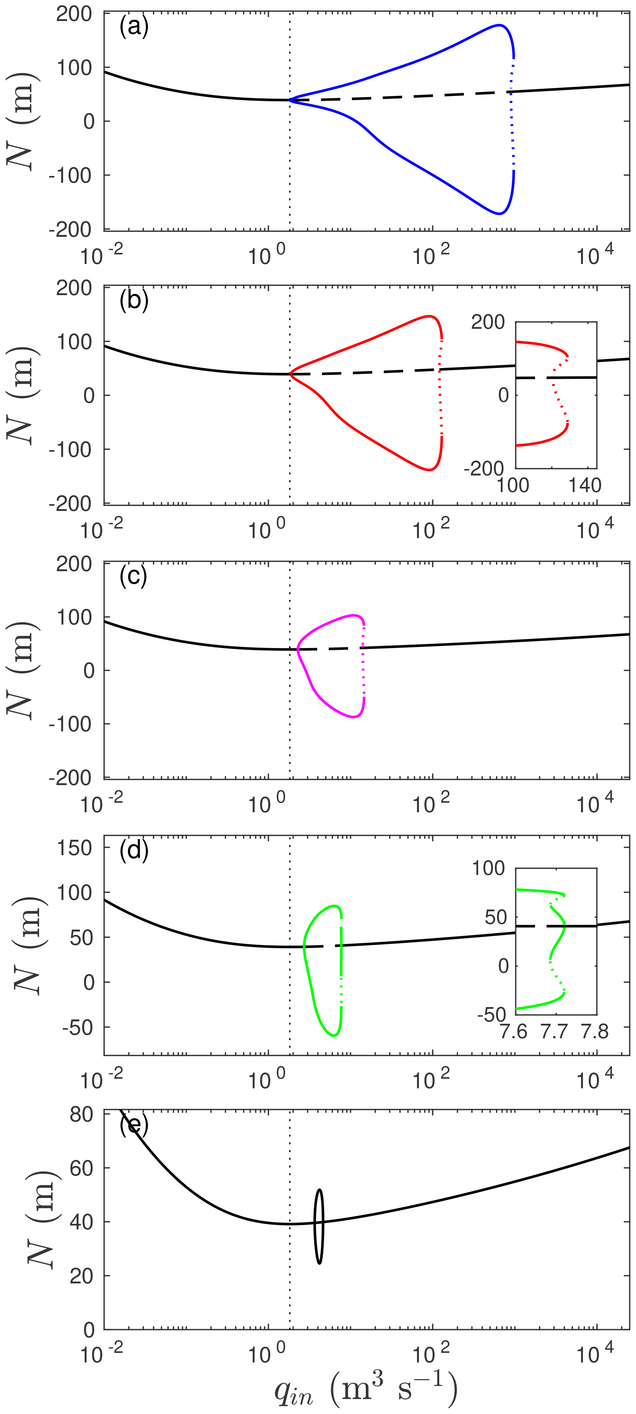
Figure 5 Bifurcation diagrams for L=50 km and V_p=4 (a), 0.8 (b), 0.16 (c), 0.112 (d), and 0.094 (e) km². Plotted are stable (solid black) and unstable (dashed black) steady-state N, as well as minimum and maximum N attained in stable (solid coloured) and unstable (dotted coloured) periodic solutions. The insets in (b) and (d) show details, while the vertical dotted line marks the value of q_in at which the conduit becomes channel-like.

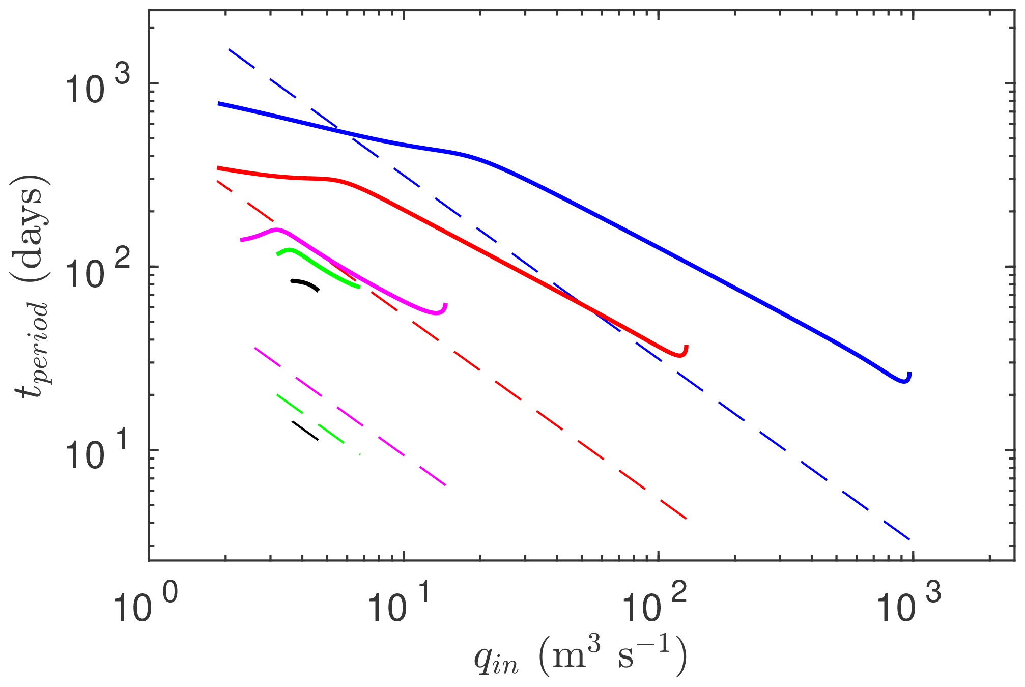
Figure 6 The period of stable periodic solutions where they exist for the same parameter values as in Fig. 5. The colour scheme is the same as for the coloured curves in Fig. 5, where only the stable portion of the periodic solution curves is shown. The dashed line here represent the asymptotic solution for the period of oscillation, Eq. (14).

In all cases, an unstable steady state corresponds to a limit cycle. As q_in crosses the lower critical value at which instability first occurs (associated with the change in the steady-state conduit from cavity- to channel-like behaviour), a limit cycle of small amplitude is formed, with that amplitude growing progressively as q_in increases, and the emerging limit cycle is an oscillation around an unstable steady state. This is consistent with a supercritical Hopf bifurcation (Wiggins, 2003).

As the upper critical value of q_in is approached, the stability analysis of Sect. 3.1 predicts that the steady state returns to stability. As this happens, we see that the amplitude of oscillations only shrinks continuously back to zero for the smallest value of ${\overline{V}}_p$ considered (in which case the upper critical value corresponds to another supercritical Hopf bifurcation). In Fig. 5a–c, the amplitude of stable periodic solutions continues to increase until values of q_in near the upper critical value are reached. The amplitude then decreases slightly with a further increase in q_in, before the periodic solution ceases to exist at a third critical value of q_in that is larger than the threshold at which the steady state has become stable again, as shown in more detail in the inset in Fig. 5b. (In technical terms, this is known as a saddle-node bifurcation of the Poincaré map of the dynamical system 2; see Wiggins, 2003.) Where this abrupt disappearance of the stable periodic solution occurs, it is accompanied by an unstable periodic solution near the upper critical value of q_in, corresponding to a subcritical Hopf bifurcation. Figure 5d (see inset) represents an exotic exception to this, where there are two stable periodic solutions for a small interval of q_in.

The nature of the Hopf bifurcations at the stability boundaries in Fig. 2 can be determined more quickly than by the numerical continuation method used above, using a weakly non-linear stability analysis (see Sect. S3.3 of the Supplement). This allows us to map out in Fig. 2 where that boundary corresponds to a supercritical Hopf bifurcation, in whose vicinity a small-amplitude stable periodic solution emerges (stability boundaries shown as a solid curve), and where the Hopf bifurcation is subcritical and the small-amplitude periodic solution is unstable (dashed stability boundary). As in the few samples shown in Fig. 5, we see that the lower critical value of q_in is always supercritical, while the upper critical value is generally subcritical, except at low V_p.

We can also compute the period of the drainage oscillations, that is, the recurrence interval of floods. Figure 6 shows the period of the stable periodic solutions shown in Fig. 5 as a function of water supply rate q_in, using the same colouring scheme to distinguish different values of V_p. Perhaps unsurprisingly, large inflow rates q_in correspond to more rapid flood cycles, and large reservoir volumes correspond to floods repeating more slowly, albeit with a larger amplitude.

There is a significant caveat here: in many cases, the limit cycle solutions we have computed predict that N becomes negative during the cycle of reservoir filling and draining. This is not something that the models are designed for. Instead of the conduit expanding through creep, as occurs in the models (1) and (2) when N<0, we expect that the glacier should instead detach from the bed, and a sheet flow of water initiates the outburst flood in this case; prototypes of models for this behaviour can be found in Schoof et al. (2012), Hewitt et al. (2012) and Tsai and Rice (2010).

Figure 7 The stability boundary of Fig. 2 for L=50 km plotted in black, with the region of parameter space in which the steady state is unstable shown in grey. The red curve is the set of parameter combinations (q_in,V_p) for which there is a periodic solution that reaches a minimum effective pressure of N=0. The minimum effective pressure becomes negative inside the region delineated by the red curve. Note that this region extends slightly beyond the right margin of the grey-shaded unstable region: this small strip is the region where stable limit cycles coexist with steady-state solution; see for instance the inset of Fig. 5b. The dotted–dashed curve is the asymptotic formula 15 for the threshold value of q_in at which negative N is first attained.

It is important to know where in parameter space the outburst flood mechanism would in reality change away from conduit growth due to cavities becoming channel-like at the end of the refilling phase and instead involve water separating ice from bed at vanishing effective pressure. The boundary between these two regimes should correspond to the location in parameter space where the minimum effective pressure during the flood cycle is zero. Figure 7 shows that parameter regime boundary, computed numerically (Sect. S3.4 of the Supplement) and superimposed on the stability boundary plot of Fig. 2. Clearly, sheet-flow-initiated floods (in which the glacier starts to float at the start of the outburst flood) are favoured at high water input rates and smaller reservoir volumes, where the conduit is less able to adjust to the rapid refilling of the reservoir.

3.4 Asymptotic solutions

We can also address limit cycle solutions through asymptotic methods in some parametric limits in our model. The most relevant limit for real glacier-dammed lakes is likely to be that of a relatively large reservoir that is filled relatively slowly, but where water supply is not so small as to allow the conduit to be cavity-like in steady state (in which case the reservoir would be drained steadily, without a flood cycle): this is the case of large V_p and moderate but not small q_in and is described in Appendix A and, in detail, in Sect. S4 of the Supplement. This region of parameter space lies in the upper left of the unstable region of Fig. 7, between the near-vertical solid black line and the solid red curve.

In brief, the asymptotic solution confirms that there is a periodic flood cycle that the system very quickly settles into and that the flood cycle consists of three distinct stages. During the main flood stage, the evolution of the conduit is rapid and dominated by dissipation-driven melt c₁qΨ and creep closure v_c(S,N) in Eq. (2a), and water input q_in to the lake is much smaller than outflow q. This is followed by a long refilling phase in which the conduit has shrunk dramatically and therefore behaves as a cavity. Its size is dictated by a quasi-equilibrium in which the cavity opening term v_o(S) balances the creep closure term v_c(S,N), leading to a slow opening of the conduit as the reservoir fills and N consequently drops. Outflow q from the reservoir during this phase is insignificant, and the mass balance of the lake is dominated by inflow q_in. The refilling phase is terminated by a flood initiation phase whose length is intermediate between the main refilling phase and the rapid flood phase. During this initiation phase, the reservoir is still filling, but the conduit has enlarged sufficiently that dissipation-driven wall melting c₁qΨ starts to be significant.

Qualitatively, this solution is illustrated by the limit cycle in Figs. 3 and 4 and Fig. 9a. The asymptotic solution only becomes quantitatively accurate when V_p is large enough to be physically unrealistic for real glacier-dammed lakes (Sect. S4.4 of the Supplement); this is because the relatively large exponent n=3 in Glen's law makes the creep closure term quite sensitive to changes in N when N is small, and the initiation phase of the floods is affected significantly by this.

One of the predictions of the asymptotic solution is that the amplitude of effective pressure oscillations should be insensitive to refilling rate q_in, except close to the Hopf bifurcation at which oscillations are initiated. As a result, the flood recurrence period (which is essentially the time taken to refill the reservoir in the limit where reservoir drainage is fast) should simply be inversely proportional to q_in. Specifically, the result states that

$$\begin{array}{}\text{(14)}& \begin{array}{rl}{t}_{\mathrm{period}}& \sim {\stackrel{\mathrm{̃}}{N}}_f{c}_{\mathrm{1}}^{\mathit{\alpha }/(n+\mathrm{1}-\mathit{\alpha })}{c}_{\mathrm{2}}^{-\mathrm{1}/(n+\mathrm{1}-\mathit{\alpha })}{c}_{\mathrm{3}}^{\mathrm{1}/(n+\mathrm{1}-\mathit{\alpha })}\\ & {\mathrm{\Psi }}_{\mathrm{0}}^{(\mathrm{1}+\mathrm{2}\mathit{\alpha })/\left[\mathrm{2}\right(n+\mathrm{1}-\mathit{\alpha }\left)\right]}{V}_p^{n/(n+\mathrm{1}-\mathit{\alpha })}{q}_{\mathrm{in}}^{-\mathrm{1}},\end{array}\end{array}$$

where ${\stackrel{\mathrm{̃}}{N}}_f$ is a dimensionless constant, with a value of 1.44 for the parameters of α and n chosen here, in the limit of a large flow path length L (Sect. S4.1 of the Supplement). This asymptotic formula is overlaid onto the numerically computed periods in Fig. 6; it should be clear that the asymptotic formula performs poorly for the relatively moderate values of V_p used here. This should not be a surprise since Fig. 5 demonstrates that, for the same values of V_p, the amplitude of oscillations is in fact sensitive to the inflow rate q_in.

The same asymptotic solution also provides an estimate for the inflow rate q_in at which zero effective pressure is first reached during the flood cycle, and our model ceases to be physically realistic as described above. The estimate is given by an analysis of the flood initiation phase (Sect. 4.4 of the Supplement) as

$$\begin{array}{}\text{(15)}& \begin{array}{rl}{q}_{\mathrm{in}}& \sim {\mathit{\gamma }}_{\mathrm{c}}{c}_{\mathrm{1}}^{(n+\mathrm{1})/\left(\mathit{\alpha }n\right)}{c}_{\mathrm{2}}^{-\mathrm{1}/n}{c}_{\mathrm{3}}^{(n+\mathrm{1})/\left(\mathit{\alpha }n\right)}{\mathrm{\Psi }}_{\mathrm{0}}^{\mathrm{3}(n+\mathrm{1})/\left(\mathrm{2}\mathit{\alpha }n\right)}\\ & (u_{\mathrm{b}}{h}_{\mathrm{r}}{)}^{-(\mathit{\alpha }-\mathrm{1})(n+\mathrm{1})/\left(\mathit{\alpha }n\right)}{V}_p,\end{array}\end{array}$$

where γ_c≈0.25 for the values of α and n chosen here. This critical inflow rate as a function of V_p is superimposed on Fig. 7. The formula above is in general an underestimate of the value of q_in at which zero effective pressures are reached but clearly gives the correct scaling of how that value relates to V_p.

We are also able to construct a second asymptotic solution for the opposite case of a large water supply rate q_in (Sect. S5 of the Supplement). This solution is valid towards the right-hand edge of the grey region in Fig. 7 and predicts rapid oscillations in the reservoir level (or effective pressure) whose amplitude slowly evolves to a steady value. These rapid oscillations however invariably involve effective pressure changing from negative to positive. As discussed above, such solutions are clearly not physically viable, and the model must be amended to take account of ice–bed separation.

4 The spatially extended model

The analysis above provides a comprehensive picture of the lumped model (2). Here, we consider how well that lumped model represents the behaviour of its more complete, spatially extended counterpart (1). We begin by recreating the stability boundary diagrams of Fig. 2. The method by which the latter were computed explicitly (Sect. S3.1 and S3.2 of the Supplement) cannot be applied directly to the extended model (1), since we have no closed-form solution to a linearized version of the model analogous to Eq. (9). Instead, we grid the $(q_{\mathrm{in}},{\overline{V}}_p)$ parameter space used in Fig. 2 finely. For each $(q_{\mathrm{in}},{\overline{V}}_p)$ pair, we discretize the model (1), compute steady states and perform a linear stability analysis numerically as described in Schoof et al. (2014, Appendix B); this allows us to delineate regions of instability, although in a less sophisticated way. We adapt that method for the transient non-linear calculations in Figs. 9–11 by solving Eqs. (B1)–(B2) of the same Appendix in Schoof et al. (2014) using a backward Euler step.

Figure 8 The stability boundaries of Fig. 2 with L=50 km (a), 250 km (b) and 10 km (c) plotted as black lines; unstable regions in the lumped model (2) are marked in grey. Solid black circles indicate parameter combinations for which the steady-state solution to the full model (1) is stable, and small dots indicate that the full model is unstable. The magenta markers in panel (a) indicate parameter values for which the evolution of the full, spatially extended model has been computed up to finite amplitude (Figs. 9–11). The red curve in panel (a) is the same boundary as in Fig. 7, indicating where negative effective pressures are encountered in the lumped model. The dashed, coloured horizontal lines in (a) show the values of V_p used in Fig. 5, using the same colouring scheme as the periodic orbits in the latter figure.

Results are shown in Fig. 8. It is clear that the lumped model consistently underestimates the range of parameter values over which steady drainage is unstable. The onset of instability at the transition from cavity- to channel-like conduit behaviour remains robust except for small domain lengths L (Fig. 8c), where the system appears to be unstable for combinations of small storage capacities ${\overline{V}}_p$ and inflow rates q_in. The lumped model typically underestimates instability at low storage capacities and at large flow path lengths L. The latter is particularly significant since we have previously attributed stabilization to the effect of incipient reservoir drainage reducing the hydraulic gradient along the flow path and therefore reducing flow through the conduit.

While stabilization at large water input rates q_in does eventually occur, this happens at values that can be several orders of magnitude larger than predicted by the lumped model, especially for large flow path lengths L. Furthermore, for a given storage capacity ${\overline{V}}_p$, the lumped model predicts that there is a single interval of inflow rate values q_in over which instability occurs. The spatially extended model by contrast has two or more such intervals for most values of ${\overline{V}}_p$, with a narrow region of stability between (the diagonal bands of solid black diamonds in Fig. 8a and b).

To understand this discrepancy better. we have solved for the non-linear evolution of the drainage system as described by the spatially extended model (1) for the parameter values indicated by magenta circles in Fig. 8a.

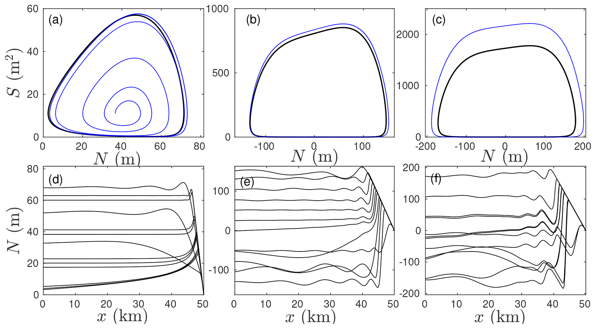
Figure 9 Each column represents one of the magenta markers in Fig. 8a. For each column, V_p=4 km² and L=50 km, while q_in=10.9 m³ s⁻¹ (panels a and d, marker A in Fig. 8.), 218.4 m³ s⁻¹ (panels b and e, marker B) and 655 m³ s⁻¹ (panels c and f, marker C). The top row (a–c) displays phase planes of $\left(N\right(\mathrm{0},t),S(\mathrm{0},t\left)\right)$ for the full model (1) (blue) superimposed on the phase plots for the lumped model (2) (black). The bottom row shows snapshots of N(x,t) against x for periodic solutions of the full model at intervals of 93 d (d), 5.5 d (e) and 4.6 d (f).

The three smallest values of q_in all correspond to unstable steady states in the lumped model (2), and we can compare spatially extended and lumped solutions. Figure 9 shows results. While the spatially extended solution is an infinite-dimensional dynamical system and strictly speaking cannot be visualized using a phase plane, we can overlay plots of conduit size S(0,t) at the upstream end of the conduit against effective pressure N(0,t) at the same location onto the S–N phase plot for the lumped model. This is shown in the top row of panels. In all three cases, the extended model settles into a limit cycle, and for small and intermediate q_in, we find good agreement between extended and lumped models. This only breaks down as we approach the upper critical value of q_in at which the lumped model stabilizes.

The lower row of panels in Fig. 9 shows snapshots of N(x,t) against x for the corresponding limit cycle shown in the top panel of the same column. For the smaller two values of q_in, we see that pressure gradients $\partial N/\partial x$ are moderate away from the glacier terminus and therefore do not contribute significantly to the hydraulic gradient Ψ. This was the basis for the reduction of the spatially extended model (1) to the lumped form (2) and explains the good agreement. For larger q_in, effective pressure N(x,t) along the conduit starts to develop wave-like structures, causing the approximation of negligible pressure gradients to break down, and the discrepancy between lumped and extended model grows.

Figure 10 Finite-amplitude evolution of the instability for the magenta dot marked “D” in Fig. 8a. (a) The maximum of N(x,t) along the flow path plotted against time t. (b) The maximum of S(x,t) with respect to x plotted against t (c) snapshots of S(x,t) at intervals of 0.93 d towards the end of the simulation (d) snapshots of N(x,t) at the same points in time as in (c). Note the logarithmic vertical scale in (c).

The extended model remains unstable beyond the stability boundary of the lumped model, but our numerical solutions no longer support the conclusion that the system necessarily settles into a limit cycle. Figure 10 shows the evolution of the system for V_p=408 m³ Pa⁻¹ s⁻¹ (a lake with a surface area of 4 km²) and $q_{\mathrm{in}}=\mathrm{2.18}\times {\mathrm{10}}^{\mathrm{3}}$ m³ s⁻¹ as in the magenta marker labelled “D” in Fig. 8a (the fact that this is an inflow rate of biblical proportions is not as relevant as it may at first seem, as we discuss in Sect. 5 below). Figure 10a and b show the growth of rapid oscillations in the maxima of N and S along the flow path over time, but without the growth becoming bounded. Figure 10c and d show snapshots over the last two oscillations in the computation. Note that the vertical scale in Fig. 10c is logarithmic. What we see is that conduit size develops an aneurysm-like, massively enlarged feature near the terminus, blocked by a narrow constriction that requires an extremely large pressure gradient to overcome. The simulation eventually terminates when the solver fails to converge, and it is unclear whether this is merely a computational problem or indicates that the true continuum solution becomes pathological or ceases to exist.

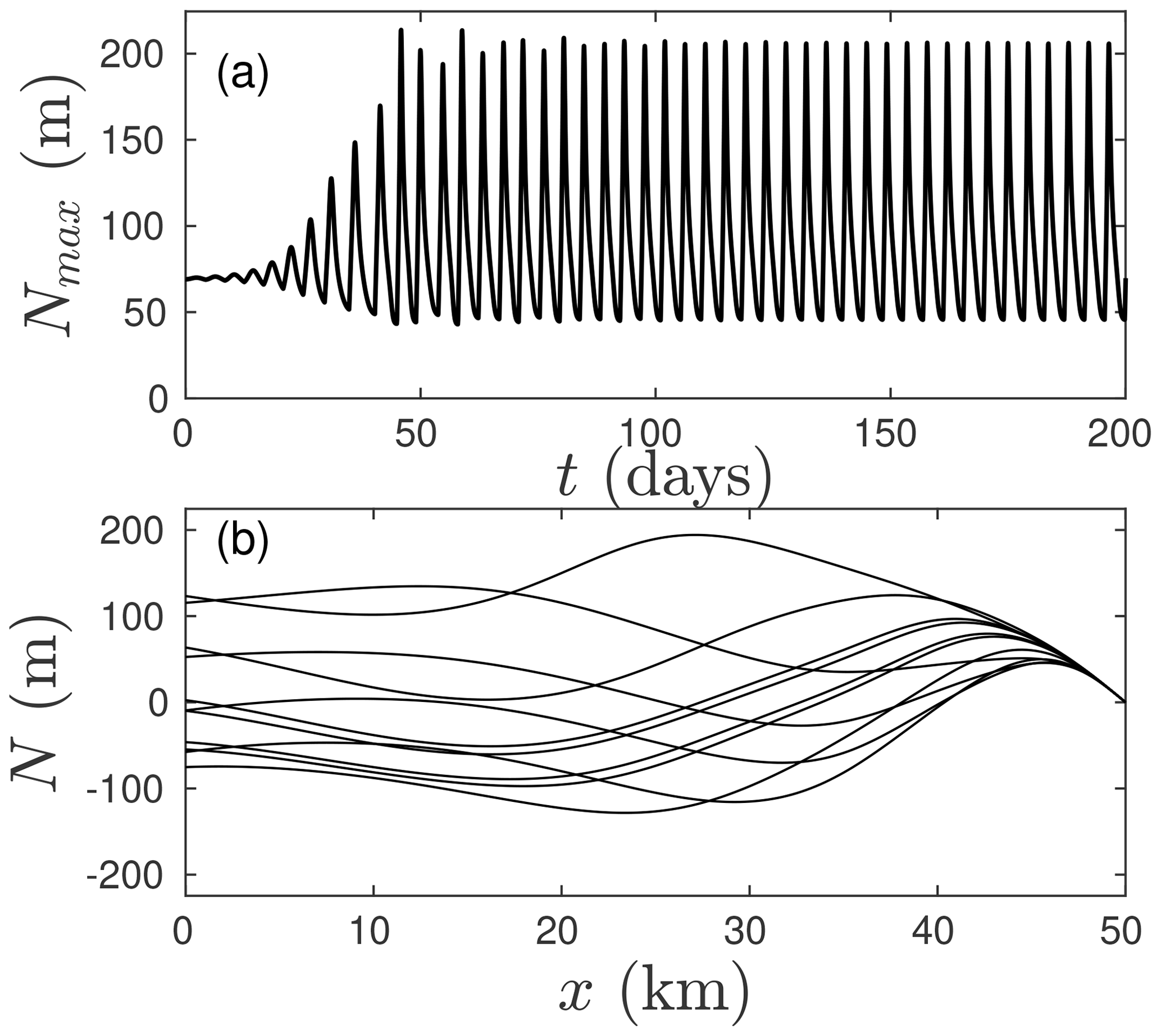
Figure 11 Finite-amplitude evolution of the instability for the magenta dot marked “E” in Fig. 8a. (a) The maximum of N(x,t) along the flow path plotted against time t. (b) Snapshots of N(x,t) at the same points in time as in (c).

For even larger q_in, a narrow band of stable values is passed and a different instability ensues as shown in Fig. 11. This instability appears to lead to bounded growth, again marked by rapid oscillations whose amplitude first grows and then saturates, and significant pressure gradients along the flow path.

Once again, a key observation is that the spatially extended model predicts negative effective pressures long before any kind of limit cycle is reached for all but one of the solutions shown and that the discrepancies between lumped and spatially extended models occur only where this is the case. Moreover, they occur for water supply rates to the reservoir that far exceed values that would be plausible for typical glacier-dammed lake systems: the lumped model appears to be robust for the latter. This includes the prediction by the lumped system of where overpressurization of the drainage system (N<0 in the limit cycle) first occurs.

This does not render some of the more exotic instabilities shown in Figs. 9–11 irrelevant: the parameter values we have chosen here were deliberately chosen to reflect typically large reservoirs dammed by low-angled and large glaciers. Much smaller reservoirs in shorter, more steeply angled glaciers are liable to give rise to some of these exotic instabilities, even though they lie outside the reach of standard glacier-dammed lakes.

5 Discussion

5.1 Glacier-dammed lakes and small reservoirs

We have shown that a drainage system that switches between cavity-like and channel-like behaviour spontaneously is capable of supporting periodic outburst floods from a glacier-dammed reservoir. At issue here is the initiation of the flood: as discussed by Ng (1998) and Fowler (1999), if the conduit behaves purely as a Röthlisberger-type channel, kept open only by melting due to heat dissipated in the turbulent flow of water through the channel, then the initiation of floods can be delayed more and more, without a limit cycle emerging. Both of these authors proposed that englacially routed water supplied to the channel should keep it open at a minimum size, and the migration of the flow divide within the channel as the lake fills then becomes the control on flood initiation. Our theory differs from theirs in the sense that no englacial water supply is necessary and the lake can continuously leak water through a linked-cavity-type drainage system that spontaneously becomes channel-like and undergoes runaway enlargement through dissipation-driven melting as the lake fills.

At the heart of the oscillatory behaviour of glacier-dammed lakes is that runaway growth, or instability, of a channel-like conduit, which prevents steady discharge of the water supplied to the reservoir (Nye, 1976; Ng, 1998; Fowler, 1999). As described in Schoof et al. (2014) and Sect. 3.1 above, this instability does not occur when the conduit draining the reservoir acts as a set of linked cavities: when these are capable of steadily draining the water supplied to the reservoir, no outburst floods occur.

For typical glacier-dammed lakes, moderate inflows q_in exceed the drainage capacity of a linked-cavity system, but the large storage capacity V_p ensures that the lake fills slowly compared with the timescale over which a basal conduit can evolve. The cycle of filling and draining then follows the characteristic sequence of a long filling period in which outflow from the lake is negligible, followed by a brief onset period in which the conduit starts to experience significant melt-driven enlargement but the lake level continues to rise, as well as an even shorter outburst flood in which inflow to the lake is dwarfed by drainage through the subglacial conduit. For a given lake size V_p, larger inflow rates will slowly increase the amplitude of the lake level fluctuation during the flood cycle (Fig. 5), while significantly shortening the length of the flood cycle (Fig. 6).

As in Ng (1998) and Fowler (1999), our flood initiation mechanism can also be too slow to respond to water input and lead to our models (1) and (2) predicting negative effective pressures at the upstream end of the conduit: in that case, the glacier ought to float and flood initiation is likely to take the form a sheet flow that subsequently channelizes, as explored in Flowers et al. (2004), Schoof et al. (2012) and Hewitt et al. (2012). This effect is not included in our models here, but we are at least able to give an approximate expression (valid in the limit of very large reservoir sizes V_p) for the water supply q_in at which the change in flood initiation mechanism occurs (switching between unstable conduit growth and partial glacier flotation and a sheet flow); this is Eq. (15). Adapting our model to account for this alternative flood initiation mechanism is the obvious next step to take. One straightforward adaptation of the lumped model to this effect, inspired by the model in Hewitt et al. (2012), is the following: if we suppose that lake level cannot rise beyond the point at which N=0, then the opening of an ice–bed gap must be such as to permit outflow balancing inflow to the lake at that point, which forces us to alter the constitutive relation for q once N=0. We can similarly build the possibility of flood termination due to the lake running dry at an upper bound on effective pressure at $N=N_{max}={\mathit{\rho }}_{\mathrm{i}}g\left(s\right(\mathrm{0})-b(\mathrm{0}\left)\right)$ into the model. Once the lake is fully empty, discharge q in the conduit will be the lesser of inflow into the conduit q_in (corresponding to a partially filled conduit) and the discharge the conduit would carry if it were completely filled with water. The appropriately adapted lumped model (2) is

$$\begin{array}{}\text{(16a)}& {\displaystyle }\dot{S}& {\displaystyle }=c_{\mathrm{1}}q\mathrm{\Psi }+v_{\mathrm{o}}\left(S\right)-v_{\mathrm{c}}(S,N),\text{(16b)}& {\displaystyle }-V_p\dot{N}& {\displaystyle }=q_{\mathrm{in}}-\stackrel{\mathrm{̃}}{q},\text{(16c)}& {\displaystyle }\stackrel{\mathrm{̃}}{q}& {\displaystyle }=\left\{\begin{array}{ll}max\left(q\right(S,\mathrm{\Psi }),q_{\mathrm{in}})& \text{if }N=\mathrm{0},\\ q(S,\mathrm{\Psi })& \text{if }\mathrm{0}<N<N_{max},\\ min\left(q\right(S,\mathrm{\Psi }),q_{\mathrm{in}})& \text{if }N=N_{max},\end{array}\right.\text{(16d)}& {\displaystyle }\mathrm{\Psi }& {\displaystyle }={\mathrm{\Psi }}_{\mathrm{0}}-N/L.\end{array}$$

The equivalent for the spatially extended model (1) is the channel model in Hewitt et al. (2012), with a reservoir at the upstream end. Importantly, the stability of steady-state solutions as in Sects. 3.1 and 4 is unchanged by these adaptations unless the steady state corresponds to an empty lake basin and a partially filled conduit, in which case the conduit is presumably stable since discharge in the conduit does not increase when its size is increased. The upper and lower bounds on flux introduced in the model (16) only affects the non-linear dynamics of the system, once the amplitude gets large enough. We leave the non-linear analysis of the adapted model to future work.

We have also investigated a mechanism previously identified in Schoof et al. (2014), by which flow out of a reservoir can be stabilized when the storage capacity in the reservoir is relatively small, so that typical drainage rates (comparable to the inflow rate q_in) lead to adjustment of effective pressure in the reservoir much faster than the conduit can evolve due to wall melting. The rapid response of reservoir water levels can have a large enough effect on hydraulic gradients to stabilize the flow. This is true at least for a short enough drainage system. Importantly, this happens at water throughput rates that are completely unrealistic for typical, large glacier lakes (and even these rates are underestimated by a simplified, lumped model as described in Sect. 4).

Figure 12 Stability boundary plotted in the same way as in Fig. 2, but with Ψ₀=1630 Pa m⁻¹ and $u_{\mathrm{b}}{h}_{\mathrm{r}}=\mathrm{1.05}\times {\mathrm{10}}^{-\mathrm{7}}$ m² s⁻¹, and we put L=10 000 m.

The reason why this stabilization mechanism is relevant is that it may explain why much smaller water reservoirs that are typically not recognized as lakes but nonetheless provide storage capacity (such as large moulins) do not invariably generate outburst-flood type behaviour. The stability diagram of Fig. 8 was generated for parameter values chosen to represent single reservoirs dammed by glaciers with a small (1:50) surface slope. For the more limited flow paths of 50 and 10 km length, any small reservoir like a large moulin (say, with a maximum side length of 10 m, or a base area of V_p of no more than 10⁻⁴ km²) is stable for even small discharge rates of 1 m³ s⁻¹; only a very long flow path of 250 km combined with a single such reservoir could be unstable (Fig. 8b) with (for such a large moulin) moderate flow rates of 10 m³ s⁻¹.

The picture changes significantly when we look at shorter, steeper glaciers. We can reduce the size of the parameter space that we need to sample in order to understand different glacier geometries by scaling the problem (Sect. S2.2 of the Supplement). If we change the background hydraulic gradient Ψ₀ (representing steepness) by a factor χ_Ψ and the cavity opening rate v_o (representing sliding velocity and bed roughness) by a factor χ_v, the effect on stability is equivalent to keeping Ψ₀ and v_o fixed but instead changing q_in by a factor of ${\mathit{\chi }}_{\mathrm{v}}^{-\mathrm{1}}{\mathit{\chi }}_{\mathrm{\Psi }}$, while simultaneously changing V_p by a factor of ${\mathit{\chi }}_{\mathrm{v}}^{[\mathit{\alpha }-(n+\mathrm{1}\left)\right]/\left(\mathit{\alpha }n\right)}{\mathit{\chi }}_{\mathrm{\Psi }}^{[\mathrm{2}\mathit{\alpha }n+\mathrm{3}(n+\mathrm{1}\left)\right]/\left(\mathrm{2}\mathit{\alpha }n\right)}={\mathit{\chi }}_{\mathrm{v}}^{-.73}{\mathit{\chi }}_{\mathrm{\Psi }}^{\mathrm{2.6}}$ and L by a factor of ${\mathit{\chi }}_{\mathrm{v}}^{-(\mathit{\alpha }-\mathrm{1})/\left(\mathit{\alpha }n\right)}{\mathit{\chi }}_{\mathrm{\Psi }}^{\mathrm{1}-\mathrm{3}/\left(\mathrm{2}\mathit{\alpha }n\right)}={\mathit{\chi }}_{\mathrm{v}}^{-.066}{\mathit{\chi }}_{\mathrm{\Psi }}^{.6}$.

The most significant impact here is that of steepening Ψ on the volume V_p at which stabilization or destabilization occurs. Consider the concrete example of a 10 km long glacier (Fig. 8c) and steepening its surface slope by a factor 8.5 from 1:50 to 17:100, while also reducing the cavity opening rate v_o by a factor of three due to slower sliding. In terms of stability, this is equivalent to keeping the 1:50 surface slope and original cavity opening rate but instead increasing q_in by a factor of 25.5, increasing storage capacity V_p by a factor 584 and increasing the glacier length L by a factor 3.88 (that is, to 38.8 km). In other words, we would go from Fig. 8c to something that resembles Fig. 8a (in which L=50 km rather than 38.8 km), but with a flux of 25.5 m³ s⁻¹ as indicated by axis labels in the figure representing an actual flux of 1 m³ s⁻¹ and a volume V_p of $\mathrm{5.84}\times {\mathrm{10}}^{-\mathrm{2}}$ km² actually representing a value of 10⁻³ km². At this point, a relatively modest 10 m-by-10 m reservoir may become unstable at reasonable water fluxes q_in, being located in parameter space towards the right-hand end of the stability boundary marked by solid circles in Fig. 8a. As a result, some of the more exotic manifestations of instability explored in Sect. 2.1 are more likely to be within reach of typical water input rates. Figure 12 shows the actual stability diagram for this steeper glacier using the same plotting scheme as Fig. 8.

As our discussion above indicates, relatively small, isolated storage volumes could lead to instabilities either for steeper glaciers or for very long flow paths. The latter in particular are however an unlikely scenario: take the example of 10 m-by-10 m moulin at the head of a 250 km flow path. In reality, there would most likely be many moulins spread out along the flow path instead. With this as motivation, we discuss a second exotic instability next, in which we opt for the opposite endmember of possible storage geometries by spreading out storage capacity evenly along the flow path. Much of the necessary groundwork is already in place from the analysis in Sect. 3.1.

5.2 Distributed storage: a modification of Nye's instability

In Sect. 2, we formulated a model for a single reservoir, for which Nye's instability predicts the onset of oscillations when the conduit becomes channel-like. In Schoof et al. (2014, Sect. 5), the case of spatially spread out storage capacity, for instance in the form of numerous basal crevasses arrayed along the flow path, was considered in addition to a single reservoir. A numerical linear stability analysis was used to demonstrate that instability can also occur for cavity-like conduits (which are generally stable for a single reservoir) for the case of such distributed water storage. The resulting oscillations (see Fig. 8 of Schoof et al., 2014; note that the figure captions for Figs. 8 and 9 are switched in the published paper) are likely to be analogous to those found in Dow et al. (2016) for the case of no localized subglacial lake. As in the case of a single reservoir, Schoof et al. (2014) find that there is a finite range of values q_in for which instability then occurs, only that this extends to lower values of q_in, where the conduit is cavity-like.

Here we sketch how to build on Sect. 3.1 to shed further light on the results in Schoof et al. (2014), which were built on the model

$$\begin{array}{}\text{(17a)}& {\displaystyle \frac{\partial v\left(N\right)}{\partial t}}+{\displaystyle \frac{\partial \stackrel{\mathrm{̃}}{q}}{\partial x}}& {\displaystyle }=\mathrm{0},\text{(17b)}& {\displaystyle \frac{\partial S}{\partial t}}& {\displaystyle }=c_{\mathrm{1}}q\mathrm{\Psi }+v_{\mathrm{o}}\left(S\right)-v_{\mathrm{c}}(S,N),\text{(17c)}& {\displaystyle }\stackrel{\mathrm{̃}}{q}& {\displaystyle }=q(S,\mathrm{\Psi }),\text{(17d)}& {\displaystyle }\mathrm{\Psi }& {\displaystyle }={\mathrm{\Psi }}_{\mathrm{0}}+{\displaystyle \frac{\partial N}{\partial x}}.\end{array}$$

Here v(N) is a decreasing function of N that describes storage of water per unit length of the conduit, and the rest of the notation used replicates that of the single-reservoir model (1). Below, we will denote by

$$\begin{array}{}\text{(18)}& v_p=-{\displaystyle \frac{\mathrm{d}v}{\mathrm{d}N}},\end{array}$$

the equivalent of V_p in Eq. (1). This model also requires boundary conditions; an obvious choice is a prescribed flux q=q_in at the inflow x=0, with no actual reservoir there, and again N=0 at the terminus x=L.

With a finite domain size and the proposed boundary conditions above, a steady-state solution to the model (17) will in general have spatial structure as in Schoof et al. (2014), and a linearization around that steady state, analogous to Sect. 3.1, will lead to a boundary value problem that is not amenable to a closed-form solution. To avoid this, we concentrate here on shorter length scales and assume that we can use the model (17) with periodic boundary conditions at these scales. This yields a spatially uniform steady-state solution defined implicitly by Eq. (7a) combined with $q_{\mathrm{in}}=q(\overline{S},\overline{\mathrm{\Psi }})$ and $\overline{\mathrm{\Psi }}={\mathrm{\Psi }}_{\mathrm{0}}$, where q_in is the prescribed flux through the system. This is closely analogous to Eq. (7) but simpler, as the hydraulic gradient here does not contain the gradient term retained in Eq. (7c).

Linearizing as $N=\overline{N}+N^{\prime }\exp (ikx+\mathit{\lambda }t)$, $S=\overline{S}+S^{\prime }\exp (ikx+\mathit{\lambda }t)$, we find an analogue to the problem (8) as

$$\begin{array}{}\text{(19a)}& {\displaystyle }\begin{array}{rl}& -{\overline{v}}_p\mathit{\lambda }{N}^{\prime }+ik{q}_S{S}^{\prime }-k^{\mathrm{2}}{q}_{\mathrm{\Psi }}{N}^{\prime }=\mathrm{0},\\ & \mathit{\lambda }{S}^{\prime }-(c_{\mathrm{1}}{q}_S\overline{\mathrm{\Psi }}+v_{\mathrm{o},S}{S}^{\prime }-v_{\mathrm{c},S})S^{\prime }\end{array}\text{(19b)}& {\displaystyle }-\left[ik{c}_{\mathrm{1}}(q_{\mathrm{\Psi }}\overline{\mathrm{\Psi }}+\overline{q})-v_{\mathrm{c},N}\right]N^{\prime }=\mathrm{0},\end{array}$$

using the same notation as in Sect. 3.1. The eigenvalue λ is again given by an equation of the form (9), but now with a₁ and a₂ given by

$$\begin{array}{}\text{(20a)}& {\displaystyle }{a}_{\mathrm{1}}& {\displaystyle }=(c_{\mathrm{1}}{q}_S\overline{\mathrm{\Psi }}+v_{\mathrm{o},S}-v_{\mathrm{c},S})-{\overline{v}}_p^{-\mathrm{1}}{k}^{\mathrm{2}}{q}_{\mathrm{\Psi }},\text{(20b)}& {\displaystyle }{a}_{\mathrm{2}}& {\displaystyle }={\overline{v}}_p^{-\mathrm{1}}\left\{k^{\mathrm{2}}\left[c_{\mathrm{1}}{q}_S\overline{q}+q_{\mathrm{\Psi }}(v_{\mathrm{c},S}-v_{\mathrm{o},S})\right]+ik{q}_S{v}_{\mathrm{c},N}\right\}.\end{array}$$

The only term that differs intrinsically from Eq. (10) is a₂, which now has an imaginary part. We see that the real part of a₂ is still invariably positive, so the real part of a₁−4a₂ is smaller than a₁. However, we can no longer conclude that the real part of λ has the same sign as a₁.

We can identify two mechanisms for instability. The first is essentially the same as Nye's melt–drainage feedback: the more storage capacity there is, the smaller all the terms containing k are in Eq. (20) for a given wavenumber k, and the more likely the first term $(c_{\mathrm{1}}{q}_S+v_{\mathrm{o},S}-v_{\mathrm{c},S})$ in the definition of a₁ is to dominate the eigenvalue λ, leading to instability for a channel-like system. To increase the size of the potentially stabilizing terms therefore requires larger wavenumbers k, and a larger range of short wavelengths is likely to be unstable.

A second instability mechanism can occur if the conduit is cavity-like with $(c_{\mathrm{1}}{q}_S+v_{\mathrm{o},S}-v_{\mathrm{c},S})<\mathrm{0}$ and therefore a₁<0. It is still possible to have an eigenvalue with a positive real part and hence instability, because a₂ has a non-zero imaginary part. One particular case in which an instability due to this term may occur is with limited storage capacity (so ${\overline{v}}_p^{-\mathrm{1}}$ is large) and at an intermediate wavelengths range (so k is small but not too small). Then it is possible, purely by controlling the size of the storage capacity ${\overline{v}}_p$, to ensure that $a_{\mathrm{1}}^{\mathrm{2}}-\mathrm{4}{a}_{\mathrm{2}}\sim -i\mathrm{4}{\overline{v}}_p^{-\mathrm{1}}{q}_S{v}_{\mathrm{c},N}k$ and

$$\begin{array}{}\text{(21)}& \mathit{\lambda }\sim \pm (\mathrm{1}-i)\sqrt{{\displaystyle \frac{{\stackrel{\mathrm{̃}}{v}}_p^{-\mathrm{1}}k{q}_S{v}_{\mathrm{c},N}}{\mathrm{2}}}}.\end{array}$$

Full details can be found in Sect. 6 of the Supplement. Choosing the plus (+) sign ensures an eigenvalue with a positive real part. Importantly, this instability corresponds to a growing wave that propagates, in this case downstream as the imaginary part of λ is then negative. It is also of the same size as the real part, so propagation is not slow. This unstable wave is not the result of Nye's instability as the conduit is cavity-like. Instead, it is the result of an interaction between the dependence of the conduit closing rate on effective pressure and the dependence of water drainage (which affects effective pressure through water storage) on conduit size.

To make these considerations more concrete, Fig. 13 shows the stability diagram for the system (17) for the parameter values used in Fig. 8, but with the upstream reservoir V_p replaced by distributed storage v_p as indicated on the vertical axis. Compared with Fig. 8, it should be clear that there are larger regions of parameter space that exhibit instability for cavity-like conduits (to the left of the vertical portion of the red stability boundary). As in the case of a single reservoir, a larger domain length is destabilizing, but a larger total storage volume is in general necessary to cause instability for channelized systems compared to a localized reservoir.

For instance, for longest flow path of L=250 km, one 10 m-by-10 m moulin per kilometre of flow path (equivalent to $v_p={\mathrm{10}}^{-\mathrm{4}}$ km) is marginally unstable at q_in=10 m³ s⁻¹ in Fig. 13b, while a single such moulin at the upstream end of the conduit is unstable at even larger q_in. Put another way, compared with a single reservoir, distributed storage favours instability at smaller q_in. The possibility of oscillatory flow occurring at low q_in outside of the melt season due to this instability was previously explored in Schoof et al. (2014).

Figure 13 Stability of steady-state solutions to the model (17) with parameters given by Table 1 and L=50 km (a), 250 km (b) and 10 km (c). Solid black circles indicate parameter combinations for which the steady-state solution to the full model (1) is stable, and small dots indicate that the full model is unstable. The red curves indicate the stability boundaries of the lumped model (2) with V_p=v_pL.

6 Conclusions

As demonstrated previously using a much more restricted sweep of parameter space in Schoof et al. (2014), we have shown that drainage systems capable of switching spontaneously between channel- and cavity-like behaviour are stable in the presence of a localized water reservoir at low and high water throughput, with an unstable intermediate range of water fluxes. In that range, spontaneous oscillations in reservoir level will occur, driven by Nye's (1976) instability mechanism driving outburst floods. These outburst floods turn out to be regular, periodic oscillations in water level at least at low-to-moderate water input, where a simplified, lumped model of reservoir drainage generally reproduces the results of a more sophisticated, spatially extended drainage model. At high water throughput rates, our results are more equivocal as to the emergence of such limit cycles in the model used; in any case, the model necessarily breaks down physically (as opposed to mathematically) because it predicts that the oscillations will invariably reach negative effective pressures and therefore flotation of the ice dam at such large throughput rates.

It is worth pointing out that part of our focus has been on the emergence of limit cycle solutions in order to identify how the flood initiation mechanism can prevent flood magnitude from increasing progressively from cycle to cycle as observed in Ng (1998) and Fowler (1999), as well as to present an alternative mechanism for suppressing the continued growth in amplitude from that considered by Fowler (1999), whose lake is necessarily sealed between floods. The alternative mechanism here is the ability of a cavity-like drainage system that remains open during the reservoir recharge phase to switch to a channelized drainage mode.

The fact that we illustrate this by showing evolution towards a limit cycle is not at odds with the chaotic behaviour observed by Kingslake (2015) using a variant of Fowler's (1999) model: the chaotic behaviour is intrinsically the result of a time-varying water input to the reservoir, which we have not studied in this paper. It is entirely possible, and in fact likely, that our model will also behave chaotically under such time-varying water input rates q_in(t). The point of demonstrating that limit cycles emerge was rather to underline that the growth of Nye's (1976) instability is bounded in our model without having to appeal to additional physics.

The lower cut-off to the drainage instability that leads to outburst floods corresponds to the drainage system switching to a cavity-like state under steady flow conditions when water input to the reservoir can be drained steadily by those cavities. The mechanism for the cut-off at high water throughput rates is harder to identify. The lumped model predicts that the high sensitivity of water level in the reservoir to the evolution of the draining conduit will induce water pressure gradients that reduce flow as the conduit grows and therefore suppress its enlargement due to heat dissipation. The threshold at which this happens is however significantly underestimated by the lumped model relatively to its spatially extended counterpart, which develops more wave-like instabilities at higher water throughput rates.

In closing, we have also investigated how wave-like instabilities can occur when the water reservoir is not localized but spread out or “distributed” along the flow path (for instance, in the form of many small reservoirs like basal crevasses). This type of instability was first observed in Schoof et al. (2014) and persists even where water throughput is insufficient to lead to channel-like behaviour. Adapting the stability analysis performed on a model with localized storage, we have shown that Nye's instability persists but also that a second instability mechanism emerges, in which a phase shift between water storage and flux that causes water to accumulate in regions where effective pressure is already low arises.

Future work is likely to focus on capturing the role of overpressurization of the drainage system in initiating and mediating the instability driving outburst floods, since flood initiation at water pressures below flotation is confined to a relatively small part of parameter space, and the model predicts that reaching zero effective pressure and initiation by partial flotation of the ice dam is likely to be common.

Appendix A: Asymptotic solutions for large lakes with moderate inflow

This appendix provides only a brief sketch of the derivation of an asymptotic solution for a limit cycle solution in the case where the reservoir volume is large and inflow is sufficient to ensure that the reservoir cannot be drained by a cavity-like conduit but also that the conduit size evolves much faster than the timescale over which the reservoir fills. Full details are given in Sect. S4 of the Supplement.

The solution is developed from a parametric limit of the model (2) with Eq. (1g), where we assume S₀=∞. We scale as $N^{**}=N/[N{]}^{\prime }$, $S^{**}=S/[S{]}^{\prime }$, $t^{**}=t/\left[t\right]$, where the scales are defined through $[S{]}^{\prime }/[t{]}^{\prime }=c_{\mathrm{1}}{c}_{\mathrm{3}}[S{{]}^{\prime }}^{\mathit{\alpha }}{\mathrm{\Psi }}_{\mathrm{0}}^{\mathrm{3}/\mathrm{2}}=c_{\mathrm{2}}[S{]}^{\prime }[N{{]}^{\prime }}^n$ and $V_p[N{]}^{\prime }/[t{]}^{\prime }=c_{\mathrm{1}}[S{{]}^{\prime }}^{\mathit{\alpha }}{\mathrm{\Psi }}_{\mathrm{0}}^{\mathrm{1}/\mathrm{2}}$. Substituting and omitting the asterisks immediately, we obtain

$$\begin{array}{}\text{(A1a)}& {\displaystyle }\dot{S}& {\displaystyle }=S^{\mathit{\alpha }}|\mathrm{1}-\mathit{\nu }N{|}^{\mathrm{3}/\mathrm{2}}+\mathit{\delta }-S|N{|}^{n-\mathrm{1}}N,\text{(A1b)}& {\displaystyle }\dot{N}& {\displaystyle }=-\mathit{ϵ}+S^{\mathit{\alpha }}|\mathrm{1}-\mathit{\nu }N{|}^{-\mathrm{1}/\mathrm{2}}(\mathrm{1}-\mathit{\nu }N),\end{array}$$

where $\mathit{\nu }=[N{]}^{\prime }/({\mathrm{\Psi }}_{\mathrm{0}}L)$, $\mathit{\delta }=u_{\mathrm{b}}{h}_{\mathrm{r}}/\left(c_{\mathrm{2}}\right[S{]}^{\prime }\left[N{{]}^{\prime }}^n\right)$ and $\mathit{ϵ}=q_{\mathrm{in}}/\left(c_{\mathrm{1}}\right[S{{]}^{\prime }}^{\mathit{\alpha }}{\mathrm{\Psi }}_{\mathrm{0}}^{\mathrm{1}/\mathrm{2}})$.

We assume that the exponents n and α satisfy $n+\mathrm{1}>\mathit{\alpha }>\mathrm{1}$, in which case the asymptotic solution we develop is valid when

$$\mathit{\delta }\ll \mathit{ϵ}\mathit{\lesssim }{\mathit{\delta }}^{(\mathit{\alpha }-\mathrm{1})(n+\mathrm{1})/\left(\mathit{\alpha }n\right)}\ll \mathrm{1}$$

and ν≲1.

The main flood phase is described by omitting terms of O(δ) and O(ϵ)

$$\begin{array}{}\text{(A2a)}& {\displaystyle }\dot{S}& {\displaystyle }=S^{\mathit{\alpha }}|\mathrm{1}-\mathit{\nu }N{|}^{\mathrm{3}/\mathrm{2}}-S|N{|}^{n-\mathrm{1}}N,\text{(A2b)}& {\displaystyle }\dot{N}& {\displaystyle }=S^{\mathit{\alpha }}|\mathrm{1}-\mathit{\nu }N{|}^{-\mathrm{1}/\mathrm{2}}(\mathrm{1}-\mathit{\nu }N),\end{array}$$

where matching with the initiation phase described later requires that $(N,S)\to (\mathrm{0},\mathrm{0})$ as $t\to -\mathrm{\infty }$. The transformation $P=N/S$ allows the system (A2) to be recast in such a way as to demonstrate that the orbit into the fixed point (0,0) is unique, so there is only one flood phase solution. The orbit terminates at a finite $N={\stackrel{\mathrm{̃}}{N}}_f$ as t→∞; this then sets the amplitude of the lake level fluctuations that give the asymptotic formula (14) for the flood cycle period.

The refilling phase is described by the rescaling $\stackrel{\mathrm{̃}}{N}=N$, $\stackrel{\mathrm{̃}}{S}={\mathit{\delta }}^{-\mathrm{1}}S$ and $\stackrel{\mathrm{̃}}{t}=\mathit{ϵ}(t-t_f)$, where t_f is the time of the last flood. At leading order,

$$\begin{array}{}\text{(A3a)}& {\displaystyle }\mathrm{0}& {\displaystyle }=\mathrm{1}-\stackrel{\mathrm{̃}}{S}|\stackrel{\mathrm{̃}}{N}{|}^{n-\mathrm{1}}\stackrel{\mathrm{̃}}{N},\text{(A3b)}& {\displaystyle \frac{\mathrm{d}\stackrel{\mathrm{̃}}{N}}{\mathrm{d}\stackrel{\mathrm{̃}}{t}}}& {\displaystyle }=-\mathrm{1};\end{array}$$

conduit size is quasi-steady and cavity-like, while lake level evolves purely because of inflow.

The refilling phase ends as N→0 and cavity size becomes large. The relevant rescaling becomes

$$\begin{array}{ll}{\displaystyle }\widehat{N}& {\displaystyle }={\mathit{\delta }}^{-(\mathit{\alpha }-\mathrm{1})/\left(\mathit{\alpha }n\right)}\stackrel{\mathrm{̃}}{N},\widehat{S}={\mathit{\delta }}^{(\mathit{\alpha }-\mathrm{1})/\mathit{\alpha }}\stackrel{\mathrm{̃}}{S},\\ {\displaystyle }\widehat{t}& {\displaystyle }={\mathit{\delta }}^{-(\mathit{\alpha }-\mathrm{1})/\left(\mathit{\alpha }n\right)}(\stackrel{\mathrm{̃}}{t}-N_f)\end{array}$$

and gives at leading order

$$\begin{array}{}\text{(A4a)}& {\displaystyle }\mathit{ϵ}{\mathit{\delta }}^{-(\mathit{\alpha }-\mathrm{1})(n+\mathrm{1})/\left(\mathit{\alpha }n\right)}{\displaystyle \frac{\mathrm{d}\widehat{S}}{\mathrm{d}\widehat{t}}}& {\displaystyle }={\widehat{S}}^{\mathit{\alpha }}+\mathrm{1}-\widehat{S}|\widehat{N}{|}^{n-\mathrm{1}}\widehat{N},\text{(A4b)}& {\displaystyle \frac{\mathrm{d}\widehat{N}}{\mathrm{d}\widehat{t}}}& {\displaystyle }=-\mathrm{1},\end{array}$$

where we have assumed $\mathit{ϵ}\sim {\mathit{\delta }}^{(\mathit{\alpha }-\mathrm{1})(n+\mathrm{1})/\left(\mathit{\alpha }n\right)}$; the alternative case of ϵ∼δ is described in the Supplement. The key to Eq. (A4) is that it predicts finite-time blow-up in $\widehat{S}$ at some finite $\widehat{N}={\widehat{N}}_{\mathrm{c}}$ that depends purely on the value of $\mathit{ϵ}{\mathit{\delta }}^{-(\mathit{\alpha }-\mathrm{1})(n+\mathrm{1})/\left(\mathit{\alpha }n\right)}$. This is the smallest value of effective pressure (rescaled, of course) that is reached during the drainage cycle. The larger $\mathit{ϵ}\sim {\mathit{\delta }}^{(\mathit{\alpha }-\mathrm{1})(n+\mathrm{1})/\left(\mathit{\alpha }n\right)}$, the smaller and eventually more negative ${\widehat{N}}_{\mathrm{c}}$ becomes; there is therefore a critical value of $\mathit{ϵ}\sim {\mathit{\delta }}^{(\mathit{\alpha }-\mathrm{1})(n+\mathrm{1})/\left(\mathit{\alpha }n\right)}$ at which ${\widehat{N}}_{\mathrm{c}}=\mathrm{0}$. When rendered in dimensional form, this value gives the formula (15).