Seasonal transition dates can reveal biases in Arctic sea ice simulations

Arctic sea ice experiences a dramatic annual cycle, and seasonal ice loss and growth can be characterized by various metrics: melt onset, breakup, opening, freeze onset, freeze-up, and closing. By evaluating a range of seasonal sea ice metrics, CMIP6 sea ice simulations can be evaluated in more detail than by using traditional metrics alone, such as sea ice area. We show that models capture the observed asymmetry in seasonal sea ice transitions, with spring ice loss taking about 1–2 months longer than fall ice growth. The largest impacts of internal variability are seen in the inflow regions for melt and freeze onset dates, but all metrics show pan-Arctic model spreads exceeding the internal variability range, indicating the contribution of model differences. Through climate model evaluation in the context of both observations and internal variability, we show that biases in seasonal transition dates can compensate for other unrealistic aspects of simulated sea ice. In some models, this leads to September sea ice areas in agreement with observations for the wrong reasons.

1 Introduction

Metrics of seasonality have been underutilized in evaluating sea ice in climate models due to a lack of long-term observational products, the required daily model output, and the complexities in defining seasonal Arctic sea ice transitions. However, new process-based metrics for model evaluation are much needed; the spread between climate model projections of sea ice area has been on the order of millions of square kilometers in Coupled Model Intercomparison Project (CMIP) Phases 3, 5, and 6 (Stroeve et al., 2012; SIMIP-Community, 2020), while the causes of the model spread remain largely unknown. Furthermore, the sources of model biases can be obscured by models that show realistic sea ice areas for the wrong reasons. Seasonal sea ice transitions can provide additional process-based metrics to assess climate models. Newly available observational data (Steele et al., 2019) and model output from CMIP6 models (Notz et al., 2016) allow such model assessment for the first time. In this study, we assess how different metrics of seasonal sea ice transitions are represented in models and observations and evaluate how these metrics can inform our understanding of simulated Arctic sea ice throughout the year. To do this, we utilize observations and 16 global climate models, including three sets of ensembles with at least 30 members. Using this rich dataset, we evaluate model biases in the context of both the observed sea ice state and multiple simulated representations of internal variability.

2 Background: seasonal transitions in the Arctic sea ice cover

Arctic sea ice exhibits a large annual cycle, with a difference of approximately 8×10⁶ km² between the maximum area reached in March and the minimum area in September. From spring to fall, the sea ice experiences various stages of transition forced by both the atmosphere and the ocean (Steele et al., 2010; Persson, 2012; Ballinger et al., 2019). In the spring, clouds formed by northward warm air advection trap downwelling longwave radiation, initiating melt on the surface of the sea ice or in the snowpack on top of it (Persson, 2012; Ballinger et al., 2019). As liquid water collects on the snow and sea ice, it forms melt ponds. Melt ponds decrease the albedo of the surface: snow-covered ice has an albedo of 0.85, while the albedo of melt ponds ranges between 0.1 and 0.5 (Perovich et al., 2002). Shortwave absorption causes thermodynamic ice loss, and regional studies show that top melt dominates during the early summer (Steele et al., 2010). As the ice breaks up, larger areas of open ocean facilitate greater solar absorption (the albedo of open water is 0.07; Pegau and Paulson, 2001) and ice divergence. Energy is absorbed by the surface ocean (Timmermans, 2015), and as solar heating declines in the late summer, ice melt becomes dominated by bottom melt (Steele et al., 2010). After the annual sea ice minimum in September, ice growth begins. Congelation ice growth along existing ice generally begins before frazil ice growth in the open ocean, meaning that areas where ice is retained throughout the summer experience earlier ice growth than areas of open water (Smith and Jahn, 2019). As fall progresses, the Arctic loses shortwave input. Temperatures decline, and ice growth continues through the winter, reaching the maximum area in March.

One metric alone cannot capture the range of seasonal transitions seen in the Arctic, so individual transitions have been characterized by many different definitions in both satellite data and models. Seasonal transition metrics are often referred to interchangeably when they are in fact defined in very different ways. Pan-Arctic satellite retrievals of seasonal sea ice transitions are largely based on passive microwave brightness temperatures. Retrieval algorithms have been created to derive pan-Arctic seasonal sea ice metrics, such as melt onset and freeze onset, directly from brightness temperatures for the entire satellite era (Markus et al., 2009; Drobot and Anderson, 2001; Belchanksy et al., 2004; Bliss and Anderson, 2014; Bliss et al., 2017). Despite great spatial and temporal coverage, melt and freeze onset dates are difficult to utilize for model evaluation. This is in part due to the variations between retrieval algorithms, which can introduce large differences in both magnitude and trends of observed melt onset dates (Bliss et al., 2017). Furthermore, brightness temperatures are not simulated in climate models, so model definitions of melt and freeze onset must be based on other simulated variables. There are multiple possible variables for diagnosing melt and freeze onset, such as surface temperature, thermodynamic ice growth, and snowmelt, and the choice of variable has been shown to impact which processes are captured by the dates as well as their comparability to satellite data (Smith and Jahn, 2019).

Another strategy for defining seasonal sea ice transitions is to create metrics based on ice concentration, a variable that has equally good spatial and temporal satellite data coverage since satellite-observed ice concentration is derived from passive microwave brightness temperatures (Comiso et al., 1997). While this introduces some error through sea ice concentration retrieval algorithms (Ivanova et al., 2015), seasonal sea ice metrics based on ice concentration provide more direct comparisons between models and observations than the current comparisons made between melt and freeze onset. Ice breakup, retreat, freeze-up, and advance have been defined using ice concentration data in satellite data (Stammerjohn et al., 2008, 2012; Serreze et al., 2016; Stroeve et al., 2016; Bliss et al., 2019) and in model studies (Barnhart et al., 2016; Wang et al., 2018). However, these studies are often difficult to compare directly since the definitions themselves vary substantially in terms of the region and date range studied, the selected threshold of ice concentration, and the criteria that the threshold must meet (e.g., last day greater than 15 % vs. less than 15 % 2 d in a row). In some cases, definitions are also created to fill specific user needs, such as seasonal navigation (Johnson and Eicken, 2016). A selection of previously used metrics defined using ice concentration is described in Table S1 in the Supplement to provide an overview.

3 Data and methods

In this study we use satellite data to evaluate the performance of 15 CMIP6 models and the Community Earth System Model Large Ensemble (CESM LE) in terms of their seasonal sea ice transitions in the Arctic from 1979 to 2014. By utilizing model ensembles, we are able to account for the role of internal variability in modeling the seasonality of Arctic sea ice. As there is no single metric that fully describes seasonal sea ice changes, we utilize a variety of metrics that have been developed for both models and observations. All seasonal transition date means and means of other sea ice variables are calculated between 66 and 84.5^∘ N in both models and satellite data in order to exclude the largest polar hole in satellite data. We define “inflow regions” as the Chukchi Sea, Barents Sea, and Greenland Sea, with the Barents and Greenland seas referred to as “Atlantic inflow regions”.

3.1 Global coupled climate models

CMIP establishes a set of common experiments for global climate model simulations to quantify how the Earth system responds to forcing as well as to identify the sources and consequences of model biases (Eyring et al., 2016). This study uses models from the most recent phase, CMIP6, in order to evaluate the current state of sea ice simulation. Models are selected for analysis based on the availability of two daily sea ice variables: sea ice concentration (CMIP6 variable name: siconc) and the surface temperature of the sea ice or snow on sea ice (CMIP6 variable name: sitemptop). Our study utilizes all CMIP6 models that met these criteria by 4 March 2020, which includes 15 models from nine different institutions (ACCESS-CM2, BCC-CSM2-MR, BCC-ESM1, CanESM5, CESM2, CESM2-FV2, CESM2-WACCM, CESM2-WACCM-FV2, CNRM-ESM2-1, CNRM-CM6-1, EC-Earth3, IPSL-CM6A-LR, MRI-ESM2-0, NorESM2-LM, NorESM2-MM). As the scope of the study is limited to the satellite era, we use the historical forcing experiment from each model for the period that overlaps with satellite data (1979–2014). All models are kept on their native grids to minimize errors related to interpolation and regridding. Ocean and ice model component details for all models are provided in Table S2 (based upon Hurrel et al., 2013; Kay et al., 2015; Boucher et al., 2018; NCC, 2018a, b; Seferian, 2018; Voldoire, 2018; Wu et al., 2018; Zhang et al., 2018; Danabasoglu, 2019a, b, c, d; Dix et al., 2019; EC-Earth-Consortium, 2019; Swart et al., 2019a, b; Voldoire et al., 2019; Wu et al., 2019; Yukimoto et al., 2019a, b; Boucher et al., 2020; DeRepentigny et al., 2020; Seland et al., 2020).

The number of available ensemble members varies by model, with some models providing as few as 3 members and others as many as 35 with the required daily variables. Here we use the first ensemble member (r1i1p1f1 or r1i1p1f2) from each model for intermodel comparisons and evaluation against satellite data. To assess the internal variability of the seasonal sea ice metrics, the two CMIP6 models with at least 30 members (CanESM5 and IPSL-CM6A-LR, hereafter referred to as IPSL) are utilized in addition to the CESM LE. All of the coupled global models have a nominal ocean resolution of 1^∘. Relevant variables are available at a daily temporal resolution for 40 members in the CESM LE, 35 members in the CanESM5, and 30 members in the IPSL. When evaluating internal variability, we utilize the first 30 members from the CESM LE and CanESM5 for comparison to each other and IPSL in order to standardize the sample size. The results are insensitive to the subsetting of ensemble members (a version of Fig. 8 using all available ensemble members is provided as Fig. S2 in the Supplement).

In previous work, the CESM LE was employed to compare multiple model definitions of melt and freeze onset (Smith and Jahn, 2019). Hence, the CESM LE is utilized here to leverage what is already known about modeled seasonal sea ice transitions in evaluating CMIP6 models even though the CESM1.1 used for the CESM LE is not a CMIP6 model and does not use CMIP6 forcing. Nonetheless, the CESM LE can be compared with the CMIP6 models over the period 1979–2014 as the CMIP5 RCP8.5 forcing is not substantially different from the CMIP6 historical forcing over the period 2006–2014 (O'Neill et al., 2016). Furthermore, the CESM LE is also a useful addition to the CMIP6 models because it adds diversity to the sea ice models used for evaluating internal variability: the CESM LE uses the CICE Version 4.0 sea ice model, while CanESM5 and IPSL both use the Louvain-la-Neuve Sea Ice Model Version (LIM Version 2.0 and LIM Version 3.0, respectively).

3.2 Satellite data

In order to evaluate the climate models against observations, we use the Arctic Sea Ice Seasonal Change and Melt/Freeze Climate Indicators from Satellite Data, Version 1 (Steele et al., 2019). This dataset includes seasonal sea ice indicators from 1 March 1979 through 27 February 2017, derived from sea ice concentration data from the NOAA/NSIDC Climate Data Record of Passive Microwave Sea Ice Concentration and brightness temperature observations from the DMSP SSM/I-SSMIS Daily Polar Gridded Brightness Temperatures. Indicators (referred to here as seasonal sea ice transition metrics) are described in Sect. 3.3. Data are gridded to a 25 km resolution grid. We calculate the sea ice area from the NOAA/NSIDC Climate Data Record of Passive Microwave Sea Ice Concentration, accessed through the Walsh et al. (2019) dataset.

3.3 Defining seasonal sea ice transitions

Establishing a set of metrics for studying the seasonality of Arctic sea ice is important for comparing models and observations as well as interpreting the relationships between transition times and other sea ice characteristics. Here we utilize a range of seasonal sea ice transition dates and periods to study multiple thermodynamic phases of the ice that may be relevant to our physical understanding of the sea ice. These metrics are summarized in Tables 1 and 2.

Table 1 Definitions of the seasonal transition dates, including the date range, timing criteria, variable, and threshold used. SIC is sea ice concentration. Definitions based on ice concentration are designed to be comparable to Steele et al. (2019) (note that day has been abbreviated to d when associated with a value).

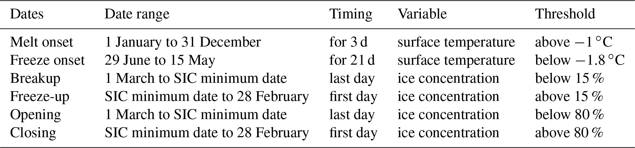
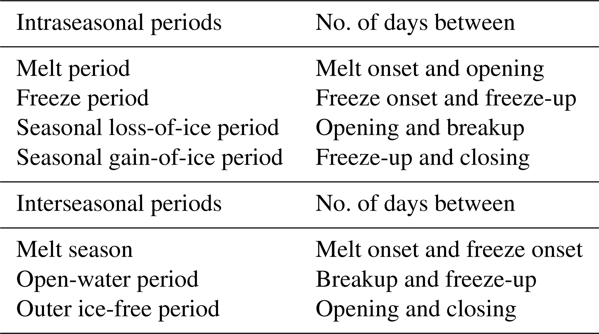
Table 2 Definitions of the periods of time between the seasonal transition dates, including shorter, intraseasonal periods of transition as well as longer, interseasonal periods. The outer ice-free period and the seasonal loss-of-ice and gain-of-ice periods were defined in Steele et al. (2019).

Figure 1 Conceptual diagram of seasonal sea ice transitions, beginning with spring melt onset and ending with fall ice closing. Transition dates (Table 1) as well as interseasonal and intraseasonal transition periods (Table 2) are labeled.

3.3.1 Melt onset, freeze onset, and the melt season

The melt season length is defined as the number of days between melt onset and freeze onset. The melt season length has been utilized as a parameter to investigate energy absorption of the Arctic surface ocean, and relationships have been found between the melt season length and sea ice extent (Stroeve et al., 2014). The metrics of melt onset and freeze onset are used to describe the first date of continuous sea ice melt and freeze at each grid cell for each year. Melt and freeze onset are meant to capture a change in phase between water and ice. For melt onset, this means water on the surface of the ice or snowpack. For freeze onset, the change in phase refers to either congelation or frazil ice growth.

In satellite retrievals, continuous melt and freeze onset are defined using the brightness temperature of the surface because brightness temperature is sensitive to the phase of water (Markus et al., 2009; Steele et al., 2019). Brightness temperatures are collected at the 19V and 37V polarizations from SMMR, SSM/I, and SSMIS sensors. Melt and freeze onset dates are derived from weighted brightness temperature parameters to determine early melt and freeze onset and continuous melt and freeze onset, and the retrieval algorithm (known as PMW) is described fully in Markus et al. (2009). In this study we use continuous melt and freeze onset because these dates are more representative of a seasonal transition in the sea ice compared to early melt onset. The advanced horizontal range algorithm (AHRA) dataset provides an alternative set of melt onset dates that are derived from passive microwave brightness temperatures using the AHRA retrieval algorithm instead of the PMW retrieval algorithm. However, the AHRA melt onset dates are more representative of early melt (Drobot and Anderson, 2001), so they are not utilized in this study.

Because climate models do not simulate brightness temperatures, another definition must be used to identify continuous melt and freeze onset dates within models. Although there is no single model definition that fully captures the processes represented by the brightness-temperature-based satellite data, recent work demonstrates that melt and freeze onset dates derived from surface temperature are comparable, particularly when considering the range of internal variability (Smith and Jahn, 2019). We therefore utilize model definitions of melt and freeze onset developed in Smith and Jahn (2019), based on the surface temperature passing below or above a given threshold. For melt onset, a threshold of −1 ^∘C is used to minimize the impacts of daily variability and maintain comparability with previous studies (Jahn et al., 2012; Mortin and Graversen, 2014). For freeze onset, a threshold equal to the freezing point of ocean water (−1.8 ^∘C) is used.

3.3.2 Breakup, freeze-up, and the open-water period

The open-water period, also known as the inner ice-free period (Bliss et al., 2019), is defined as the number of days between ice breakup and freeze-up (also commonly referred to as ice retreat and advance). The open-water period has been utilized as a metric to study variability and trends in the sea ice (Serreze et al., 2016; Barnhart et al., 2016) and seasonal predictability of the ice (Stroeve et al., 2016).

Of the seasonal sea ice transition dates investigated here, the definitions of breakup, freeze-up, and the open-water period vary the most across the literature (Table S1). In the models, we use the definitions for breakup, freeze-up, and the open-water period used in Steele et al. (2019) to allow for comparison with observations. Of the definitions identified and described in Table S1, the Steele et al. (2019) definitions are most similar to those established by Stroeve et al. (2016). Breakup is defined as the last day that sea ice concentration passes below the threshold of 15 % between 1 March and the annual sea ice concentration minimum date (Bliss et al., 2019). Freeze-up is defined as the first day that sea ice concentration passes above the 15 % threshold between the sea ice concentration minimum date and 28 February of the following year. The open-water period is defined as the number of days between breakup and freeze-up.

3.3.3 Date of opening, date of closing, and the outer ice-free period

The outer ice-free period has been used the least frequently as a metric of Arctic sea ice seasonality, and it is based on the dates of opening and closing defined by Steele et al. (2015). The Steele et al. (2015) definitions are applied in the Steele et al. (2019) dataset, as described in Bliss et al. (2019). The date of opening is defined as the first day that sea ice concentration passes below the threshold of 80 % between 1 March and the annual sea ice concentration minimum date. Likewise, the date of closing is defined as the first day that sea ice concentration passes above the 80 % threshold between the sea ice concentration minimum date and 28 February of the following year. By definition, opening must occur before breakup, and freeze-up must occur before closing. However, dates of opening and closing are not limited solely by the existence of breakup and freeze-up dates: if ice concentration falls below or above 80 % but not below or above 15 %, there will still be an opening or closing date. This means that the areal coverage of opening and closing dates is generally larger than those of breakup and freeze-up dates.

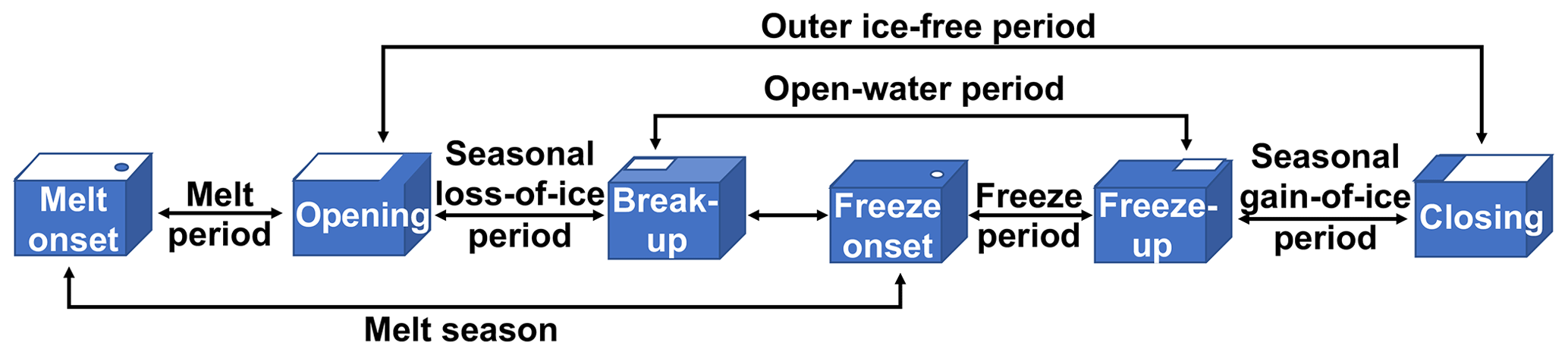
3.3.4 Melt period and freeze period

In addition to the interseasonal periods (melt season, open-water period and outer ice-free period), we describe four intraseasonal periods between the established dates (melt period, seasonal loss-of-ice period, freeze period, and seasonal gain-of-ice period; Fig. 1). The melt period is designed to capture the rate of transition between snow and sea ice to the initial appearance of open water, and it is defined as the number of days between sea ice melt onset and the date of opening. Similarly, the freeze period is defined as the number of days between freeze onset and freeze-up and is designed to describe the length of the transition between initial ice growth and the time at which an area stops being “ice-free” by exceeding the 15 % concentration threshold.

3.3.5 Seasonal loss-of-ice period and seasonal gain-of-ice period

The seasonal loss-of-ice period and the seasonal gain-of-ice period were established in Steele et al. (2019) and Bliss et al. (2019). The seasonal loss-of-ice period is defined as the number of days between sea ice opening and breakup, and the seasonal gain-of-ice period is defined as the number of days between freeze-up and closing (Bliss et al., 2019). The seasonal loss-of-ice period and the seasonal gain-of-ice period can only be calculated at grid cells where both of their respective dates exist for that year (e.g., both a date of opening and breakup are needed for a valid seasonal loss-of-ice period). The seasonal loss-of-ice period describes how quickly the ice concentration transitions from 80 % to 15 %, while the seasonal gain-of-ice period describes the rate of transition between 15 % and 80 % ice concentration.

3.3.6 Accounting for differences in spatial coverage

Variability between models depends on the selected metric for evaluating seasonal sea ice changes. Over the satellite era, opening, breakup, freeze-up, and closing each have an ice concentration boundary where there are no existing dates beyond that boundary because the ice concentration does not pass the chosen threshold. The models have different sea ice areas (Fig. S1), and the position of the ice concentration boundary varies substantially between them. It is therefore important to compare the models between each other and the satellite data in a way that captures these differences in spatial coverage. Using one ensemble member from each CMIP6 model and one ensemble member from the CESM LE, we find the mean of each characteristic at each grid cell over the period 1979–2014. We then take the spatial mean by weighing each grid cell value by its respective area between 66 and 84.5^∘ N. This value is referred to as the “satellite-era mean” and represents the pan-Arctic nature of each characteristic. Figure S3 shows the value of each transition date versus the percent area it spans, demonstrating that the spatial distribution of the modeled dates and their skews are realistic compared to satellite data. While some model differences are less pronounced when using satellite-era medians instead of satellite-era means, the results are generally insensitive to the chosen measure of center. As with the transition dates, the interseasonal and intraseasonal periods are calculated at each grid cell before taking the area-weighted spatial means.

For each seasonal transition metric, model spreads in satellite-era means are defined as the number of days between the earliest and latest simulated date. Spreads are calculated between the first ensemble member of all models as well as between the first 30 ensemble members of CESM LE, CanESM5, and IPSL. Figures 2–7 show each of the seasonal sea ice metrics derived from satellite data, one ensemble member from each available CMIP6 model, and one ensemble member of the CESM LE averaged over the period 1979–2014. Each figure includes stippling to show where the characteristic exists for less than 20 % of years in the time period.

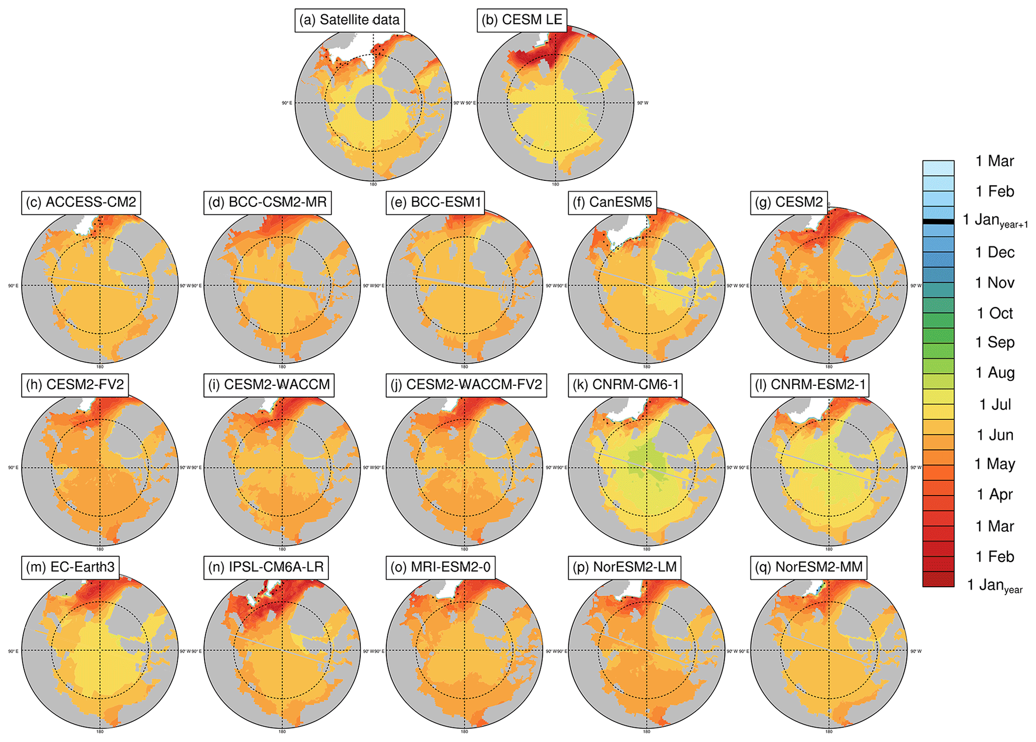
Figure 2 Melt onset dates (defined using surface temperature in the models and brightness temperatures in the satellite data) averaged over the period 1979–2014 at each grid cell using satellite data (a), the first ensemble member of the CESM LE (b), and the first ensemble member of each CMIP6 model (c–q). Stippling indicates where melt onset dates exist in less than 20 % of years in the time range. Models on tripolar grids produce plot gaps filled by gray lines.

4 Results

Results are presented in five sections. In Sect. 4.1–4.3 we describe the pan-Arctic observed and simulated seasonal sea ice transition metrics from 1979 to 2014. In Sect. 4.4 and 4.5 we compare observed and simulated relationships between the various seasonal sea ice transition metrics and sea ice area and thickness.

4.1 Spring transitions

We find that the transition from sea ice melt onset to breakup takes 2 to 3 months in both satellite data and models. Satellite data show that melt onset generally occurs between April and June over most regions of the Arctic (Fig. 2a), with the mean date of melt onset occurring on 6 June. The mean date of opening (16 July) occurs about 40 d after melt onset, and the mean breakup date (4 August) occurs 19 d after opening (Table 3). This indicates that the most time-consuming aspect of the observed spring ice loss is the transition between the start of melt on the ice or snow surface and a decline in ice area (the melt period). Once open water is present in the grid cell, the transition between 80 % ice concentration and 15 % ice concentration is faster due to energy absorption from the change in the surface albedo (Perovich et al., 2002).

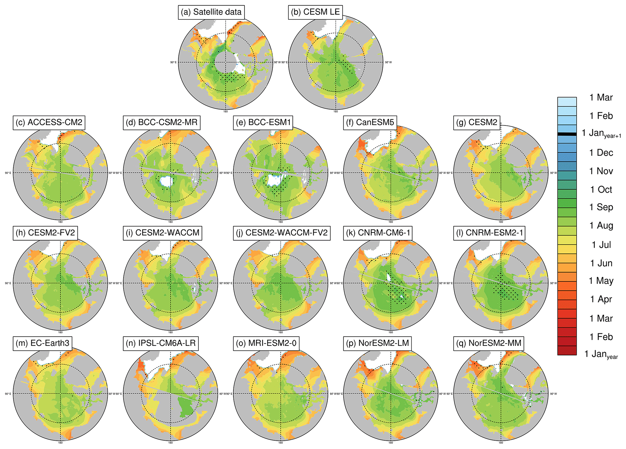
Figure 3 Opening dates (80 % ice concentration threshold) averaged over the period 1979–2014 at each grid cell using satellite data (a), the first ensemble member of the CESM LE (b), and the first ensemble member of each CMIP6 model (c–q). Stippling indicates where opening dates exist in less than 20 % of years in the time range. Models on tripolar grids produce plot gaps filled by gray lines.

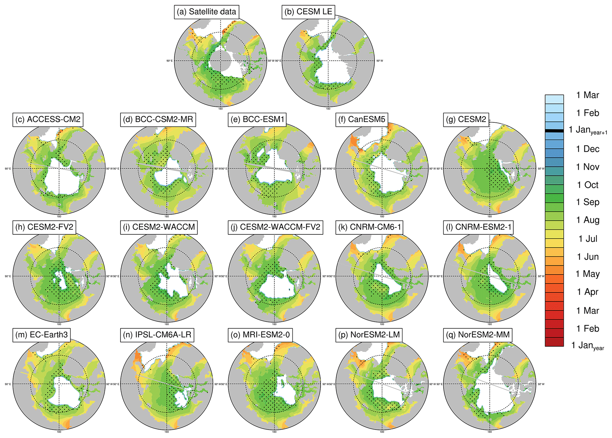
Figure 4 Breakup dates (15 % ice concentration threshold) averaged over the period 1979–2014 at each grid cell using satellite data (a), the first ensemble member of the CESM LE (b), and the first ensemble member of each CMIP6 model (c–q). Stippling indicates where breakup dates exist in less than 20 % of years in the time range. Models on tripolar grids produce plot gaps filled by gray lines.

Table 3 Pan-Arctic, satellite-era (1979–2014) means of seasonal sea ice transition dates. The satellite-era means and the all-model spreads (latest minus earliest) are calculated using the first ensemble member from each model. Models labeled with ^* show the spread in means between the first 30 ensemble members of that model. Model spreads are given in days, and all metrics are calculated between 66 and 84.5^∘ N.

Models generally agree with satellite data on the timing of spring transitions (Figs. 2–4), with mean melt onset dates over the satellite era occurring between 15 May and 18 June (observed mean date of 6 June; Table 3). Excluding the CNRM models (which show particularly late mean melt onset dates and are explored further in Sect. 4.5), the model spread (15 May–3 June) shifts earlier, and the mean melt onset dates from the remaining models all occur earlier than the satellite data. The models generally capture the spatial variation in the opening and breakup dates across the Arctic, showing a spatial standard deviation between 23 and 34 d compared to 32 d in satellite data and between 18 and 28 d compared to 27 d in satellite data, respectively (Table S3). However for the melt onset, the spatial standard deviation between models shows a difference by a factor of 4 between the models (12–47 d) compared to 20 d in the satellite data due to the very early melt onsets detected in the Atlantic inflow regions in some models (Fig. 2). Melt onset dates in the Atlantic inflow regions that fall between January and March demonstrate that melt onset at the surface of the snow pack can occur while the ice area is still expanding in those regions. This highlights that surface-temperature-based definitions, such as melt onset, capture different physical processes than sea-ice-concentration-based definitions, as was previously shown (Smith and Jahn, 2019).

In agreement with observations, all models project the mean length of the melt period to be longer than the seasonal loss-of-ice period (Table 4). The mean time between melt onset and opening (the melt period) is 32–54 d in models and 39 d in the satellite data, while the mean time between opening and breakup (the seasonal loss-of-ice period) is 14–34 d in models and 28 d in observations (Table 4, Figs. S4 and S5).

We find that for all spring transition metrics, the model spread exceeds estimations of internal variability, which show a maximum of 8 d between ensemble members (Table 3). Of the spring sea ice transition dates (melt onset, opening, and breakup), the sea ice melt onset dates show the largest spread in satellite-era means between the models (34 d; Table 3). This range is skewed late by the CNRM-ESM2-1 and CNRM-CM6-1. If the two CNRM models are excluded, the spread in mean melt onset dates is 19 d instead of 34 d, still larger than the other two spring metrics (16 d for opening and 15 d for breakup). As the CNRM melt onset dates are more than 8 d later than the other models, this also means that differences between the CNRM models and the other models are unlikely explained by internal variability alone. The CNRM models are further discussed in Sect. 4.5. Of the spring transition dates, the internal variability is highest for the melt onset dates, particularly in the marginal ice zones (Fig. 8). High variability between ensemble members in the marginal ice zones is likely related to the interannual variations in the position of the ice edge. Additionally, modeled melt onset is defined using daily surface temperature, which exhibits greater variability than daily ice concentration (Smith and Jahn, 2019).

4.2 Fall transitions

Like the spring transition metrics, we find that pan-Arctic model differences in fall transition metrics are unlikely due to internal variability alone. In the satellite data, the mean freeze onset date is 4 October, and the mean freeze-up date is 15 October. In the models, the satellite-era means of freeze onset fall between 2 October and 3 November, and mean freeze-up dates fall between 8 and 30 October. Multiple models therefore tend to show later freeze onset than observed (Figs. 5–7). The maximum range in mean freeze onset dates due to internal variability is 11 d (Table 3), and the majority of the model means (10 out of 16) are more than 11 d later than the satellite data, indicating that this delay of the mean freeze onset in the models is not only due to internal variability. Freeze-up is also generally delayed in models compared to satellite data, with 5 of the 16 models falling outside the maximum range of internal variability (9 d) of the observations. In the fall transition dates, the average standard deviation between ensemble members is highest for marginal ice zone freeze onset dates (Fig. 8). As described for melt onset, this large internal variability is due to the changing interannual position of the ice edge and the variability of surface temperature.

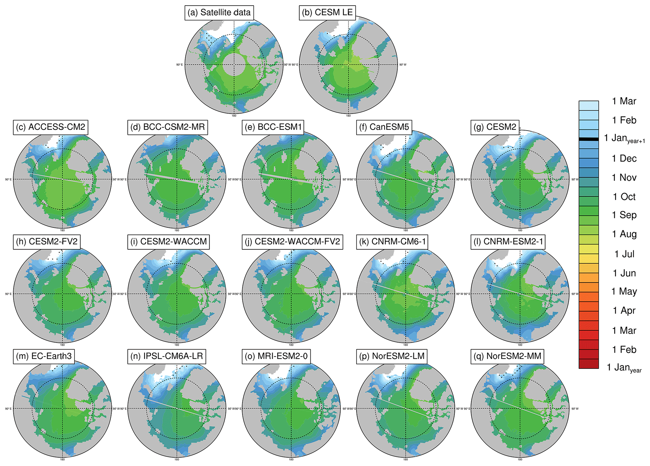
Figure 5 Freeze onset dates (defined using surface temperature in the models and brightness temperatures in the satellite data) averaged over the period 1979–2014 at each grid cell using satellite data (a), the first ensemble member of the CESM LE (b), and the first ensemble member of each CMIP6 model (c–q). Stippling indicates where freeze onset dates exist in less than 20 % of years in the time range. Models on tripolar grids produce plot gaps filled by gray lines.

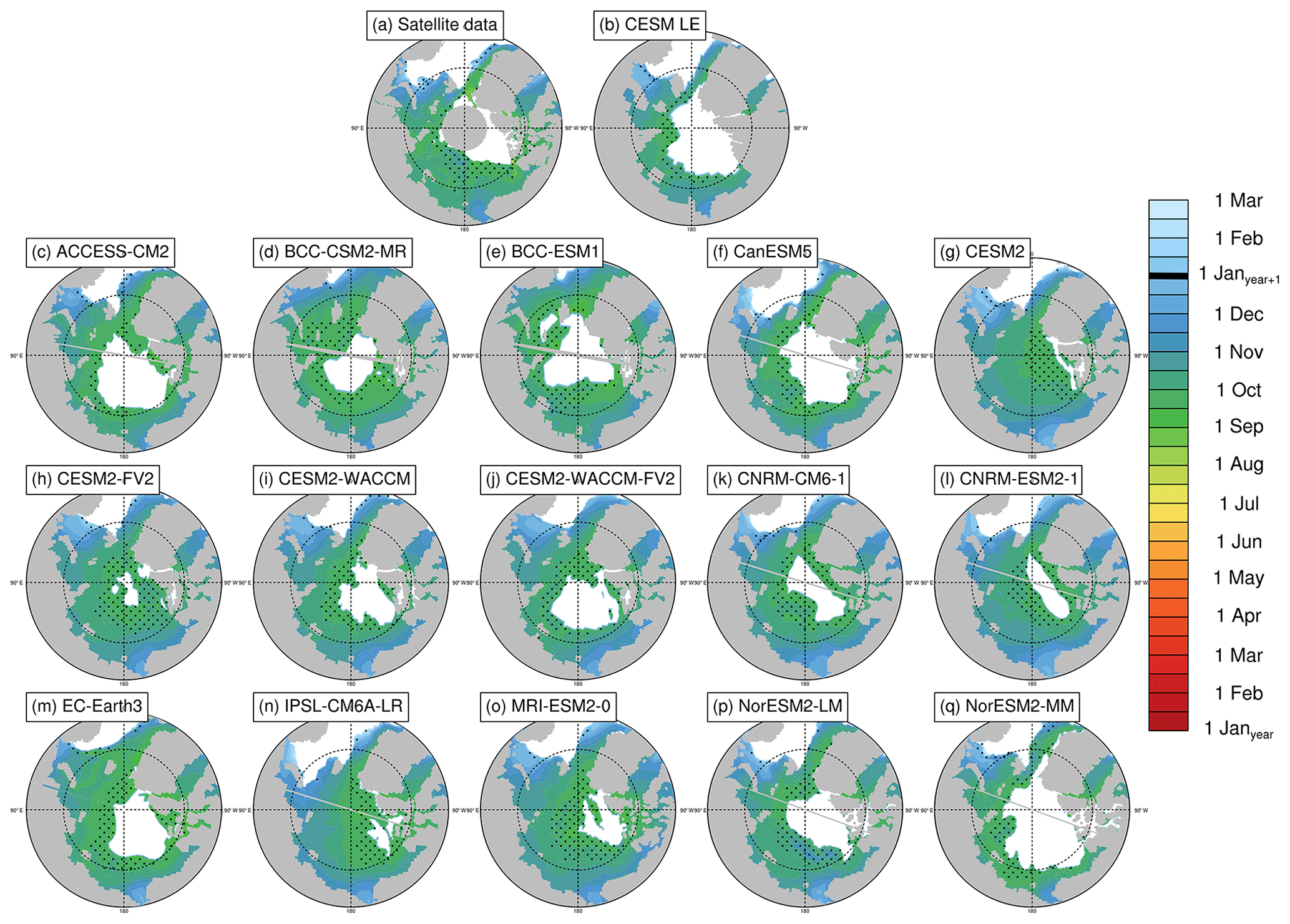
Figure 6 Freeze-up dates (15 % ice concentration threshold) averaged over the period 1979–2014 at each grid cell using satellite data (a), the first ensemble member of the CESM LE (b), and the first ensemble member of each CMIP6 model (c–q). Stippling indicates where freeze-up dates exist in less than 20 % of years in the time range. Models on tripolar grids produce plot gaps filled by gray lines.

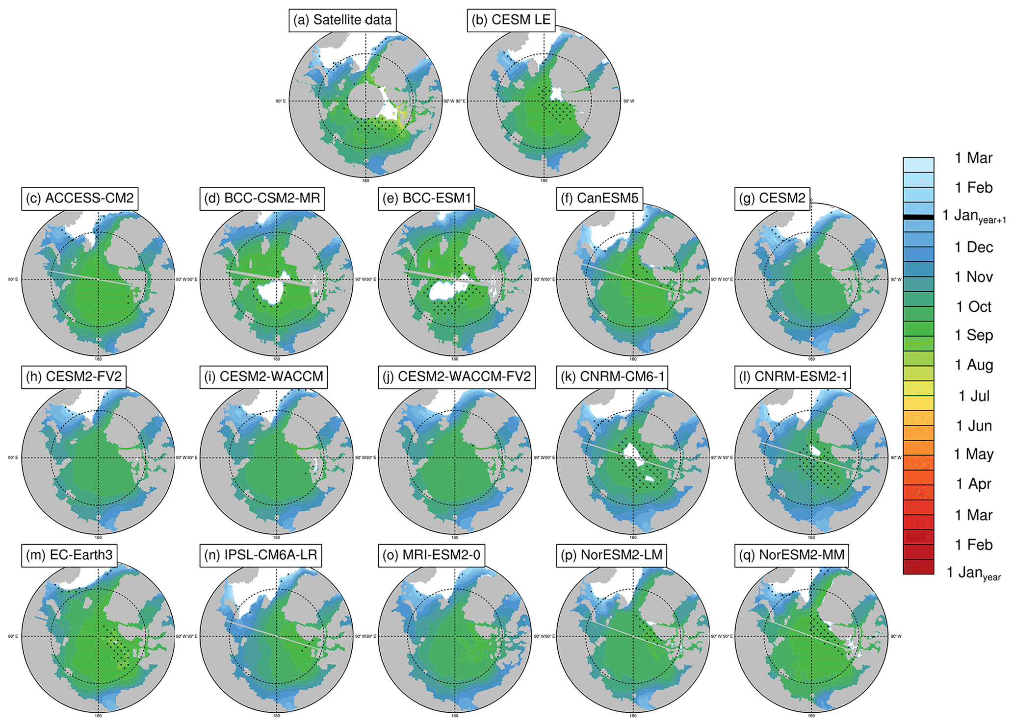
Figure 7 Closing dates (ice passes the 80 % ice concentration threshold) averaged over the period 1979–2014 at each grid cell using satellite data (a), the first ensemble member of the CESM LE (b), and the first ensemble member of each CMIP6 model (c–q). Stippling indicates where closing dates exist in less than 20 % of years in the time range. Models on tripolar grids produce plot gaps filled by gray lines.

The mean closing date occurs on 13 October in satellite data and between 4 October and 5 November in the models (Table 3). Ice freeze-up occurs before the date of closing by definition as both are defined using ice concentration, but areas closer to the central Arctic (that fall below 80 % but not 15 %) skew the mean of the closing dates earlier (in some cases earlier than the mean freeze-up date). As with the spring transition dates, models generally capture the spatial variability of the fall transition dates. Closing date standard deviations across the Arctic (which only vary by 4 d between models) do not overlap with satellite data, but freeze onset and freeze-up, which show more variation between models in terms of their standard deviations, do span the satellite data (Table S3). The mean length of the seasonal gain-of-ice period, the time between freeze-up and closing, is 15 d in satellite data and 7–14 d in models. Thus the seasonal loss-of-ice period is almost twice as long as the seasonal gain-of-ice period in both satellite data and models (Table 4, Figs. S5 and S7).

The observed time between mean freeze onset and freeze-up (the freeze period) is 9 d, with the mean freeze-up occurring before the mean freeze onset in the satellite data, leading to a negative freeze period in the mean and across most of the Arctic (Table 4, Fig. S6). This means that the transition dates do not always occur in the expected order at each grid cell, and out-of-order dates occur much more frequently for the freeze period than the melt period (Figs. S4 and S6). In satellite data, simultaneous freeze onset and freeze-up dates may in part be explained by the satellite retrieval algorithms: the PMW retrieval algorithm for freeze onset uses an 80 % ice concentration metric to derive freeze onset at locations where the date cannot be reliably derived using the weighted brightness temperature scheme (Markus et al., 2009). This would skew the freeze onset dates later and make them more similar to the closing dates. Hence, the use of ice concentration by both the freeze onset and freeze-up retrieval algorithms may contribute to cases where the dates are not sequential. A detailed assessment of this is not possible, however, as the data do not contain information on how often this backup method is employed.

In models, the definitions of seasonal sea ice metrics aim to capture thermodynamic changes in the sea ice, but the similar and sometimes out-of-order dates for freeze onset and freeze-up highlight that dynamic sea ice changes influence the ice-concentration-based transition metrics as well. While a particular grid cell may not register a persistent change in surface temperature below the threshold for freeze onset (−1.8 ^∘C), it is possible that the ice concentration of the grid cell surpasses 15 % due to dynamic transport into the grid cell, triggering the detection of freeze-up. This occurs in several models such that freeze onset occurs later than freeze-up in some parts of the Arctic, leading to negative freeze periods, as found for the satellite data (Fig. S6).

Table 4 Lengths of pan-Arctic, satellite-era (1979–2014) means of intraseasonal transition periods in days. The satellite-era means and the all-model spreads (latest minus earliest) are calculated using the first ensemble member from each model. Negative values indicate where the freeze-up date falls earlier than the freeze onset on average. Models labeled with ^* show the spread in means between the first 30 ensemble members of that model. Model spreads are given in days, and all metrics are calculated between 66 and 84.5^∘ N.

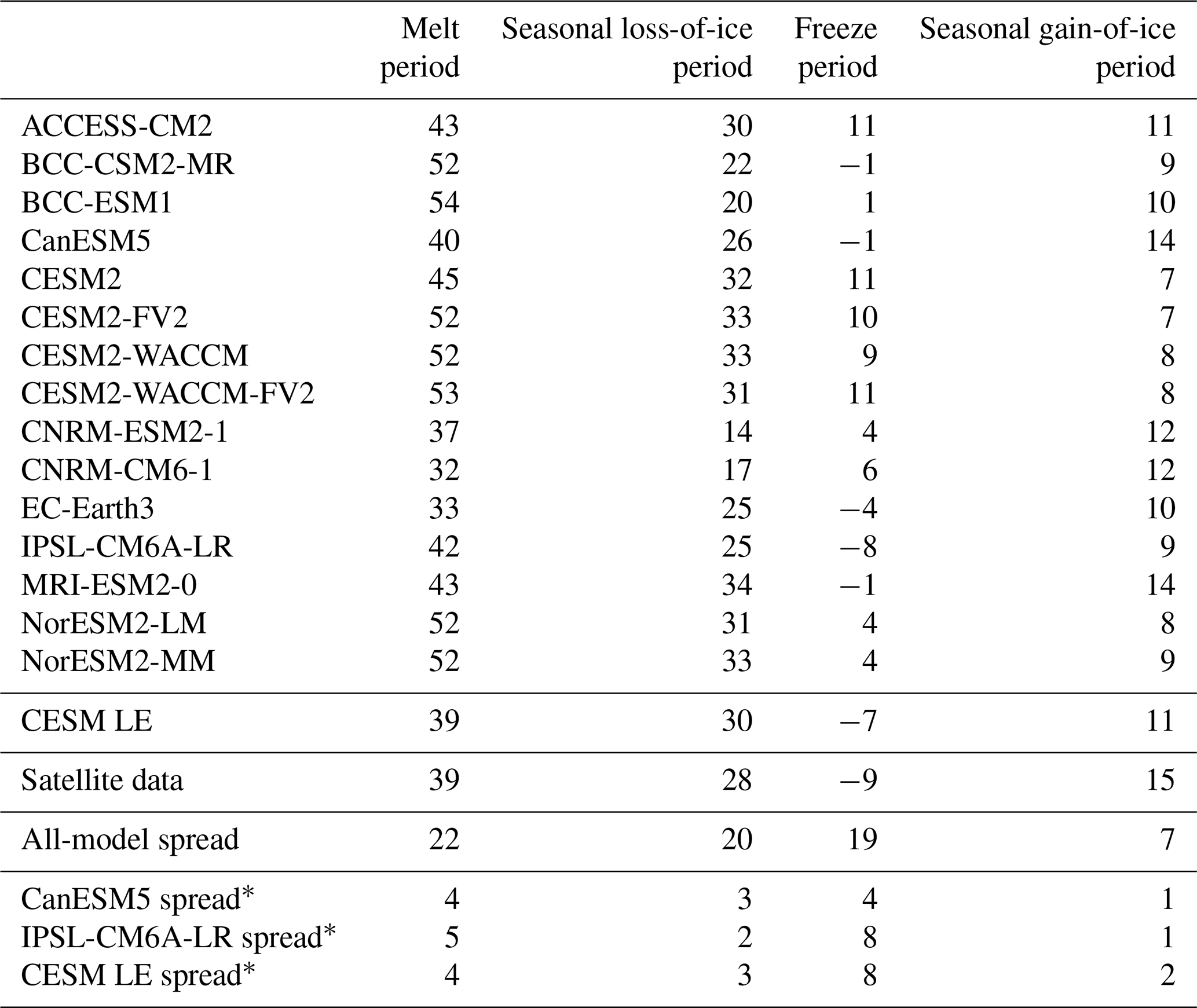
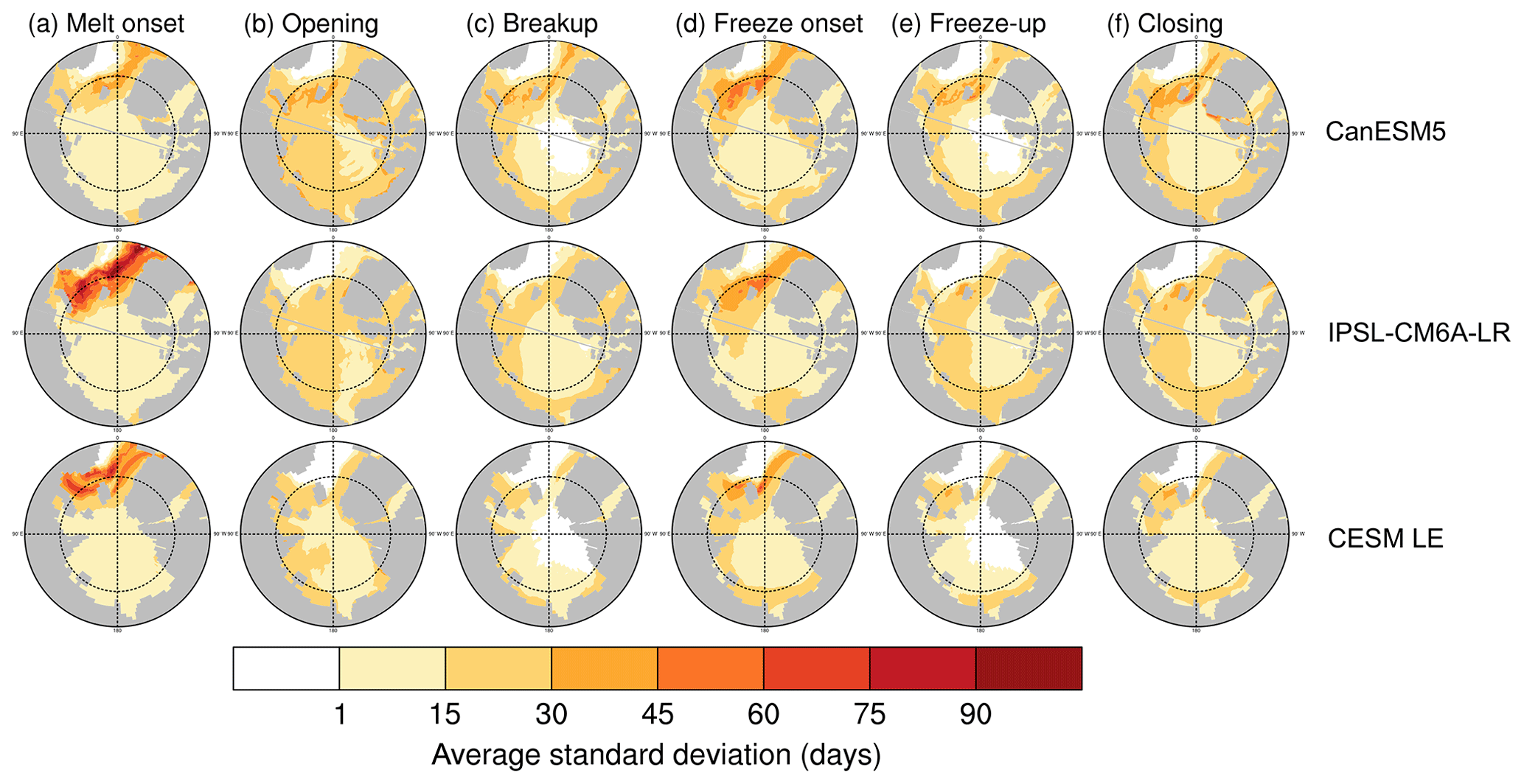
Figure 8 The average standard deviation between the first 30 ensemble members over the period 1979–2014 for (a) melt onset, (b) opening, (c) breakup, (d) freeze onset, (e) freeze-up, and (f) closing. CanESM5 is displayed in the first row, IPSL is displayed in the second row, and CESM LE is displayed in the third row. The standard deviation is calculated at each grid cell for each year, and then the average of all years is plotted for each grid cell. The same figure using all available ensemble members of each model is displayed in Fig. S2.

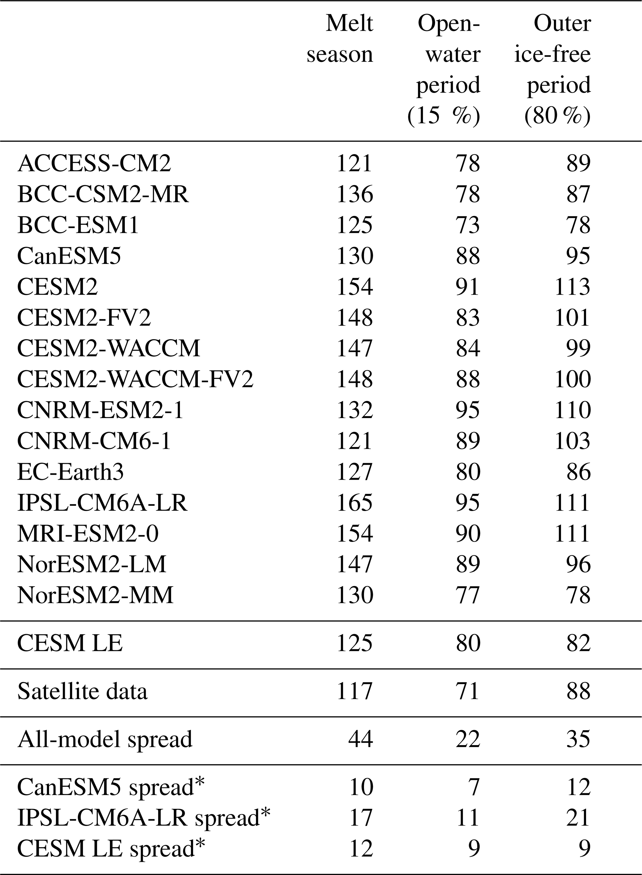
Table 5 Lengths of pan-Arctic, satellite-era (1979–2014) means of interseasonal transition periods in days. The satellite-era means and the all-model spreads (latest minus earliest) are calculated using the first ensemble member from each model. Models labeled with ^* show the spread in means between the first 30 ensemble members of that model. Model spreads are given in days, and all metrics are calculated between 66 and 84.5^∘ N.

4.3 Interseasonal transition periods

Out of the three interseasonal periods of transition (the melt season, the open-water period, and the outer ice-free period), the outer ice-free period is the only one that is consistent with satellite data. The outer ice-free period (80 % ice concentration thresholds) has an observed mean length of 88 d and model means falling between 78 and 113 d (Table 5 and Fig. S8). In contrast, the melt season length and the open-water period are too long in models compared to observations. Generally, the greatest contribution to the differences between the observed and modeled open-water period is from later-than-observed freeze-up dates. The open-water period has a mean of 71 d in the satellite data and means ranging between 73 and 95 d in the models (a spread of 22 d; Table 5 and Fig. S9). Modeled melt seasons that are too long compared to observations are also largely driven by their fall transition metric (freeze onset dates) occurring late. The observed mean melt season length is 117 d, and the model means range between 121 and 165 d (Table 5 and Fig. S10). Therefore the melt season length exhibits the largest model spread of all the interseasonal periods (44 d). This is due to larger model ranges in both melt onset and freeze onset than the other transition dates, and the contribution of each date to the model spread in melt season length is approximately equal (Table 5). The melt season length model range is also skewed high by the IPSL model, which has a mean melt season length of 165 d in its first ensemble member. This is 11 d longer than the next longest model mean, and the choice of ensemble member likely plays a role; the IPSL model has a particularly large range of internal variability in the mean melt season length (17 d compared to 10 and 12 d in the other two model sets; Table 5). While the mean melt season and open-water periods are long compared to satellite data, all modeled spatial standard deviations in interseasonal period lengths agree with satellite data (Table S4).

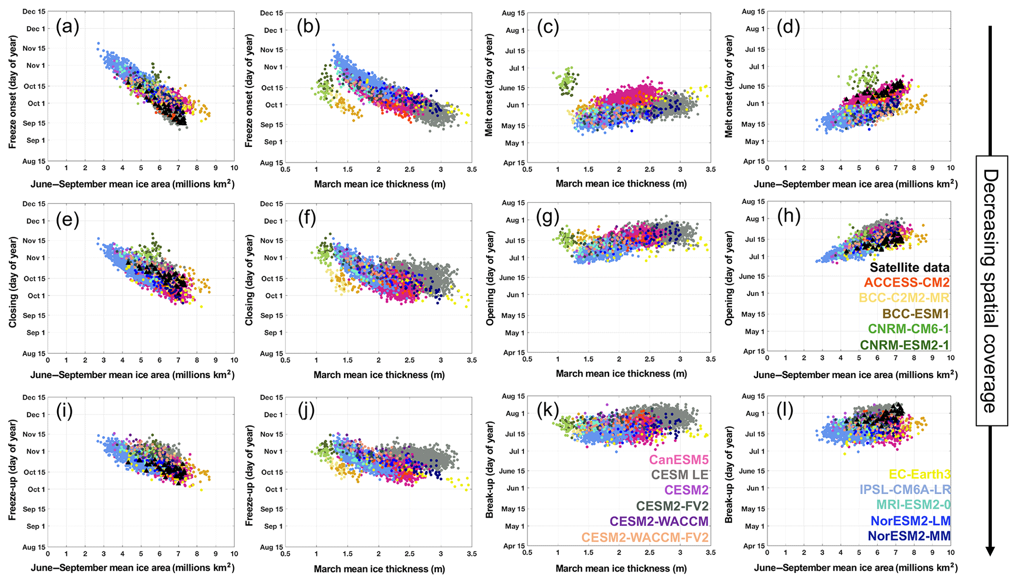
Figure 9 Scatterplots of mean seasonal sea ice transition metrics versus other ice characteristics for CMIP6 models (colors), CESM LE (gray), and satellite data (black). Each scatter point represents 1 year in one ensemble member from 1979 to 2014. Panels (a)–(d) show relationships with mean melt and freeze onset dates, panels (e)–(h) show relationships with mean opening and closing dates, and panels (i)–(l) show relationships with mean breakup and freeze-up dates. Metrics are scattered against mean summer (June–September) ice area in the first and fourth columns and March mean ice thickness in the second and third columns. All metrics are scattered against ice characteristics from the same year, except those in the second column, in which fall transition metrics are scattered against the next year's mean March ice thickness. All available ensemble members are used for CESM LE, CanESM5, and IPSL. All metrics are calculated between 66 and 84.5^∘ N. All models are represented in each panel (a)–(l), but the labels are distributed across panels (h, k, l).

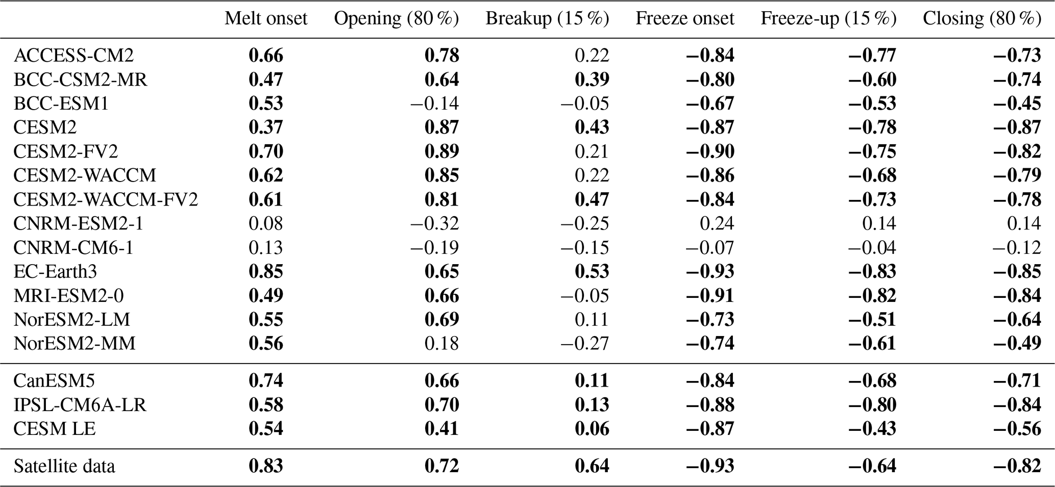
Table 6 Correlation coefficients (R values) between seasonal sea ice transition dates and mean summer (June–September) sea ice area of the same year from 1979 to 2014. Values in bold are statistically significant at the 95 % confidence level. Correlation coefficients and p values for models in the first 13 rows are determined using 1 ensemble member, for CanESM5 using all 35 ensemble members, for IPSL using all 30 ensemble members, and for CESM LE using all 40 ensemble members. All values are calculated between 66 and 84.5^∘ N.

4.4 Seasonal transitions affect sea ice area and thickness year-round

Model representations of seasonal sea ice transitions are expected to impact sea ice area and thickness because seasonal transitions are strongly linked to the ice albedo feedback (Perovich et al., 2008; Timmermans, 2015; Kashiwase et al., 2017; Perovich, 2018; Lebrun et al., 2019). Ice loss earlier in the spring has been related to later ice gain in the fall (Stroeve et al., 2014, 2016; Lebrun et al., 2019), and a weaker relationship has been described between later ice gain and earlier spring loss during the following year (Lebrun et al., 2019). Both processes favor greater areas of open ocean for longer periods each year, but little has been done to evaluate which transition metrics are most appropriate for describing pan-Arctic sea ice relationships. Here we demonstrate year-round relationships using seasonal transition dates, March mean ice thickness, and summer (June–September) mean ice area. We show that pan-Arctic relationships between seasonal transitions and other ice characteristics are most discernible using seasonal transition metrics with extensive spatial coverage (Fig. 9). Summer mean ice area is evaluated instead of the ice area of a single month in order to better represent the integrated surface energy absorption as ice area declines. Ice area and seasonal ice transition dates are practical for assessing sea ice in a pan-Arctic sense as they are reliably available for both models and observations. Discussion of the sea ice thickness here is limited to model projections since observations of Arctic sea ice thickness are temporally limited and contain large uncertainties (Bunzel et al., 2018).

We find that in satellite data, mean summer ice area (June–September) and the mean timing of freeze onset are strongly anticorrelated ($R=-\mathrm{0.93}$; Table 6 and Fig. 9). Lower summer ice area corresponds to a lower surface albedo, allowing for greater shortwave absorption by the surface ocean and increasing ocean heat content (Timmermans, 2015), delaying the freeze onset (Stroeve et al., 2014). Slightly weaker relationships exist between mean observed summer sea ice area and freeze-up ($R=-\mathrm{0.64}$) and closing ($R=-\mathrm{0.82}$). In models, the greatest agreement on the correlation between mean summer ice area and fall transition metrics is seen using the freeze onset dates, where all of the correlation coefficients that are statistically significant at the 95 % level (14 out of 16 models) are equal to or more negative than −0.67 (Table 6). Models tend to show later freeze onset than observed, as discussed in Sect. 4.2, and despite this offset the observed relationship between summer ice area and freeze onset is captured well by the models (Fig. 9). Summer ice area is generally larger in satellite data than in the models but falls within the model spread. Relationships between fall transition dates and mean summer ice thickness are similar but slightly weaker than found with ice area (Table S5).

In the models, the timing of fall transition dates is strongly correlated with the March mean ice thickness (Table 7 and Fig. 9) but does not affect the March ice area of the following year (Table S6). The differences in correlation coefficients indicate that increased heat absorption and delayed freeze onset reduce the March thickness of the ice but have a much smaller impact on the ice area. This supports past work on the Canada Basin, showing that anomalous solar heat input (Perovich et al., 2008) reduced ice thickness over the winter of 2007–2008 by 25 % (Timmermans, 2015). The strongest correlations between March ice thickness and the previous year's fall transition metrics are found between freeze onset and March ice thickness, with statistically significant correlation coefficients ranging between −0.54 and −0.92 in the models (Table 7). Because of sea ice thickness uncertainties discussed earlier (Bunzel et al., 2018), we are unable to confidently evaluate whether model biases in freeze onset impact the simulated relationship between freeze onset and March mean ice thickness compared to observations. With respect to the other fall transition metrics, we find that statistically significant correlations between March ice thickness and freeze-up or closing (which are both based on ice concentration) are less consistent between models and generally stronger for the closing dates rather than freeze-up dates (Table 7). Additionally, other relationships involving freeze-up and spring sea ice of the following year (such as the relationship between the timing of freeze-up and the next year's breakup) have been shown to be dampened by the tendency of thin ice to grow faster than thicker ice (Bitz and Roe, 2004; Lebrun et al., 2019). The growth rate of thin ice, in addition to the spatial coverage of the freeze-up dates, may limit the impact that a late freeze-up date has in reducing the following year's March mean ice thickness.

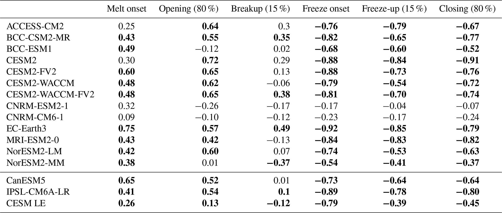
Table 7 Correlation coefficients (R values) between seasonal sea ice transition dates and March sea ice thickness from 1979 to 2014. Spring transition dates (melt onset, opening, and breakup) are correlated with March mean ice thickness from the same year, while fall transition dates (freeze onset, freeze-up, and closing) are correlated with March mean ice thickness from the following year. Values in bold are statistically significant at the 95 % confidence level. Correlation coefficients and p values for models in the first 13 rows are determined using 1 ensemble member, for CanESM5 using all 35 ensemble members, for IPSL using all 30 ensemble members, and for CESM LE using all 40 ensemble members. All values are calculated between 66 and 84.5^∘ N.

Modeled melt onset and opening dates both demonstrate weak to moderate relationships with the mean March ice thickness of the same year (Table 7 and Fig. 9). Thinner March sea ice generally corresponds with earlier mean melt onset and opening dates. For March ice thickness and melt onset, statistically significant correlations range from 0.26 to 0.75, with the CESM LE representing the weakest relationship in that range (Table 7). For March ice thickness and opening dates, statistically significant correlations range from 0.13 to 0.65 (Table 7). One might expect that thinner ice would correspond to earlier breakup dates because thinner ice is easier to melt out or split apart. However, models do not agree on the sign or statistical significance of any relationship between breakup (which are defined using ice concentration, like opening dates) and March mean ice thickness. This lack of relationship is a strong indication that the spatial coverage of breakup dates is not sufficient for describing pan-Arctic sea ice feedbacks. Increases in ice thickness after March may dampen the relationship between thin March ice and an earlier breakup date since some models show faster ice growth from March to April in areas of thin March ice rather than thick March ice (supporting past work on ice growth rates by Bitz and Roe, 2004). However, this pattern is not seen in all models and thus cannot fully account for the weakness of the relationships between March ice thickness and breakup. In addition, relationships between spring transition dates and March ice area are weaker than those between spring transition dates and March ice thickness (Table S6).

Melt onset and opening are related to mean summer ice area in both satellite data and models (Table 6 and Fig. 9; excluding the CNRM models, which are discussed in Sect. 4.5). Earlier melt is correlated with lower mean summer ice area, with a correlation coefficient of 0.83 in satellite data and a range of 0.37–0.85 in statistically significant model correlations (Table 6). Earlier opening is slightly less correlated with lower mean summer ice area with a correlation coefficient of 0.72 in satellite data, and the models range between 0.41 and 0.89 in statistically significant correlations (Table 7). Both earlier melt onset and opening dates decrease the surface albedo – the former through the formation of melt ponds and the latter through the presence of more open ocean. This once again facilitates greater surface absorption, which has been shown to increase the ocean heat content and decrease the summer sea ice cover (Stroeve et al., 2014). Relationships also exist between melt onset or opening and summer sea ice thickness (Table S5), but since the summer sea ice is already quite thin, greater ocean heat content is more likely to affect the ice area than it is in March, when ice is much thicker overall. Models do not agree on the sign or magnitude of the correlation between breakup and summer ice area, again indicating that the spatial coverage of breakup dates is insufficient for describing pan-Arctic sea ice processes.

4.5 Seasonal transitions can compensate for unrealistic sea ice characteristics

CNRM-CM6-1 and CNRM-ESM2-1 demonstrate that biases in seasonal sea ice transitions can unrealistically compensate for other sea ice biases. As mentioned in Sect. 4.1 and 4.4, the CNRM models show mean melt onset dates occurring 11–15 d later than the next latest model and 8–12 d later than those found in satellite data (Table 3). The largest differences in melt onset between the CNRM models and both satellite data and the other models are found in the central Arctic (Fig. 2k, l). While melt onset dates fall late in the CNRM models, their September ice areas are overall realistic (Voldoire et al., 2019) and fall within the spread of available models (Fig. S1). The CNRM models are the only two models (out of 16) that lack statistically significant correlations between later melt onset and larger summer ice area seen in most models and observations (Sect. 4.4). Furthermore, mean ice thickness in the CNRM models from 1979 to 2014 is much lower than in any of the other models (Fig. S1). Thus, the models' ability to produce realistic September sea ice areas likely relies on the biased seasonal transition: late melt onset acts to retain thin ice that would otherwise be lost over the summer by shortening the length of the melt season. Following melt onset, the CNRM models have mean opening and breakup dates that fall fully within the model spread, indicating that the impact of seasonal transition biases can be large, even if the biases exist only in one metric.

The cause of delayed melt onset in CNRM models is not currently clear. Melt onset is the only transition metric that captures changes at the surface of the snowpack rather than a change in ice concentration. Recent work suggests that the winter snow on the sea ice is too thick in the CNRM models, overinsulating the sea ice and preventing it from reaching realistic ice thicknesses (Voldoire et al., 2019). We find that the overinsulation in CNRM models may be more related to September–November snow thickness since the CNRM models show the largest area of 15–30 cm deep snow of all the models across this time frame (Fig. S11) but show similar snow thicknesses compared to other models during December–February (Fig. S12). Delayed melt onset could also be related to the use of the GELATO sea ice model as the CNRM models are the only models used in this study that use the GELATO model (Table S2). Since GELATO has a single snow-on-sea-ice layer and fixed albedos for dry snow and melting snow (0.88 and 0.77, respectively; Voldoire et al., 2019), simplified processes in GELATO may contribute to snow biases.

5 Conclusions

Seasonal sea ice transitions can be characterized by various metrics (melt onset, opening, breakup, freeze onset, freeze-up, and closing), and each metric represents a distinct stage of sea ice loss or gain. As such, seasonal transitions provide unique insights into Arctic sea ice processes, but they have so far been underutilized in evaluating climate models due to a lack of long-term observational products and daily model output as well as the complexities of defining seasonal transitions. Taking advantage of newly available daily model output (Notz et al., 2016) and observational data of seasonal transitions (Steele et al., 2019), we show that models capture the observed asymmetry in seasonal sea ice transitions, with spring ice loss taking about 1–2 months longer than fall ice growth (Figs. 2–7). Models also generally agree with satellite data on the timing of spring transitions. For fall transition dates, 10 out of 16 models show mean freeze onset dates later than observed such that the differences between each model's mean freeze onset date and the observed date exceed the largest estimations of internal variability (Table 3). Likewise, in 5 out of 16 models, the difference between the mean freeze-up date and the observed date exceeds the largest estimations of internal variability. Delayed freeze onset and freeze-up extend simulated melt seasons and open-water periods, respectively, making the outer ice-free period (the time between ice opening and closing) the only interseasonal period in which models consistently agree with satellite observations.

We find that differences in seasonal transitions between models are unlikely due to internal variability alone and are hence likely a reflection of model differences. Sea ice metrics are each impacted differently by internal variability: models do not agree on a metric most affected, and no single model exhibits the greatest internal variability across all metrics. Despite the uncertainty associated with internal variability, all metrics show pan-Arctic model spreads exceeding even the largest estimations of internal variability in seasonal sea ice transition metrics (Tables 3–5). The largest standard deviations between ensemble members are seen in the inflow regions for melt and freeze onset dates (Fig. 8), and this is due to the changing interannual position of the ice edge and the variability of surface temperature.

Because differences in seasonal sea ice transition metrics between models are unlikely due only to internal variability, these metrics can be used for evaluating differences between models in terms of other sea ice characteristics. We show that pan-Arctic relationships between transition metrics and sea ice area and thickness depend on the spatial coverage of the metric (Fig. 9). Out of the six transition dates, melt and freeze onset dates consistently cover the largest area of the Arctic, and they are most closely related to pan-Arctic ice area and mean thickness. Low mean summer ice area delays freeze onset (Table 6), which in turn leads to lower March ice thickness (Table 7). Thinner March ice leads to earlier melt onset and, again, low mean summer ice area (Table 6). Other relationships between sea ice area and thickness are somewhat discernible using opening and closing dates but almost indistinguishable using breakup and freeze-up dates (Fig. 9). Since the differences in relationship strengths are seen across definitions that use both surface temperature and ice-concentration-based definitions, these differences are more likely related to the spatial coverage of the seasonal sea ice transition dates rather than their defining variables (Tables 6 and 7, Fig. 9). While models tend to show later freeze onset than observed, this offset does not impact the ability of the models to produce the observed relationship between lower summer ice area and later freeze onset.

Finally, we demonstrate how seasonal sea ice transition metrics can provide context to sea ice changes that otherwise lack quantified explanations. We find that CNRM-ESM2-1 and CNRM-CM6-1 exhibit biases in both melt onset (late) and ice thickness (thin) but realistic September sea ice area, exemplifying how seasonal ice transitions can compensate for other unrealistic aspects of the sea ice. Late melt onset helps retain thin ice throughout the summer such that both CNRM models exhibit realistic September sea ice areas for the wrong reasons. Seasonal sea ice transition metrics therefore provide a process-based constraint on model simulations in addition to the commonly used September and March sea ice areas (Stroeve et al., 2012; Rosenblum and Eisenman, 2017).

To conclude, routinely saved daily sea ice variable output (in particular sea ice concentration and surface temperature) will be critical for using seasonal transitions as a new metric to assess and quantify model uncertainties associated with Arctic sea ice simulations. Since a new observational data product for these seasonal sea ice transitions now exists (Steele et al., 2019), seasonal sea ice transition dates should be used routinely in the future to better identify model biases in sea ice evolution as well as the sources of these biases.