Strain response and energy dissipation of floating saline ice under cyclic compressive stress

Understanding the mechanical behavior of sea ice is the basis of applications of ice mechanics. Laboratory-scale work on saline ice has often involved dry, isothermal ice specimens due to the relative ease of testing. This approach does not address the fact that the natural sea ice is practically always floating in seawater and typically has a significant temperature gradient. To address this important issue, we have developed equipment and methods for conducting compressive loading experiments on floating laboratory-prepared saline ice specimens. The present effort describes these developments and presents the results of stress-controlled sinusoidal cyclic compression experiments. We conducted the experiments on dry, isothermal (−10 ^∘C) ice specimens and on floating-ice specimens with a naturally occurring temperature gradient. The experiments involved ice salinities of 5 and 7 ppt, cyclic stress levels ranging from 0.04–0.12 to 0.08–0.25 MPa and cyclic loading frequencies of 0.001 to 1 Hz. The constitutive response and energy dissipation under cyclic loading were successfully analyzed using an existing physically based constitutive model for sea ice. The results highlight the importance of testing warm and floating-ice specimens and demonstrate that the experimental method proposed in this study provides a convenient and practical approach to perform laboratory experiments on floating ice.

1 Introduction

Climate change has led to an increased interest in polar sea areas and in ice behavior since accurate predictions of the evolution of the ice conditions are crucial for modeling the future climate. Warming climate has also resulted in a search for more efficient marine transit routes, production of offshore wind power, industrial operations related to extraction of hydrocarbons, and even tourism in the north (Gagne et al., 2015; Serreze and Stroeve, 2015; Kern et al., 2019). Structural loads due to sea ice make these activities challenging. In-depth understanding of the physical and mechanical properties of sea ice is required to develop tools for modeling future ice conditions and the related ice–ice and ice–wave interaction problems as well as to design safe and sustainable offshore structures (Dempsey, 2000; Feltham, 2008; Herman et al., 2019a, b; Lu and Løset, 2018; Lu et al., 2018; Ranta et al., 2017, 2018a, b; Tuhkuri and Polojärvi, 2018; Polojärvi et al., 2015; Voermans et al., 2019; Cheng et al., 2019; Li et al., 2015).

This paper studies the mechanical behavior of laboratory-prepared saline ice specimens under cyclic loading. This type of loading occurs in wave–ice and some ice–ice and ice–structure interaction problems – all important in the changing polar environment. For example, warming climate causes an increase in the amount of open water and broken ice fields, which strengthens the impact of waves on sea ice. From the perspective of pure-ice mechanics and modeling of ice, the cyclic loading experiments yield information on the elastic and viscoelastic components of strain and their dependence on the physical or microstructural characteristics of the ice. The cyclic loading tests also give insight into the fatigue of ice (Haskell et al., 1996; Bond and Langhorne, 1997; Langhorne et al., 1998; Mellor and Cole, 1981; Murdza et al., 2019; Schulson and Paul, 2009; Iliescu et al., 2017; Iliescu and Schulson, 2002).

Cyclic loading experiments on freshwater ice have been performed since the '40s (Kartashkin, 1947; Mellor and Cole, 1981) and on saline ice since the '80s (Tabata and Nohguchi, 1980; Cole, 1995; Cole and Durell, 1995; Cole et al., 1998). Cole and Durell (1995) studied the effects of temperature (from −5 to −50 ^∘C), cyclic stress amplitude (from 0.1 to 0.8 MPa) and loading frequency (from 10⁻³ to 1 Hz) on the response of laboratory-grown saline ice; the ice response was revealed to be sensitive to variations in these factors. Cole et al. (1998) investigated the response of columnar first-year sea ice to cyclic loading and found that the elastic, anelastic and viscous strains varied according to the relation between the loading and preferred c axis directions of the specimens. More recently, Heijkoop et al. (2018) conducted strain-controlled cyclic compression tests on sea ice to ascertain the variation in storage and loss compliances versus frequency. All of this earlier work has been performed using isothermal, dry specimens.

An often-overlooked issue in laboratory-scale experimentation is that most sea ice problems involve ice that is floating on water. Floating ice commonly has a through-thickness temperature gradient, resulting in a through-thickness gradient in its mechanical properties. The latter point is important to address in experimentation and modeling. The temperature gradient is implicitly taken into account when performing in situ experiments on floating ice (Langhorne et al., 2015; Smith et al., 2015; Wongpan et al., 2018). The cost of in situ experimental campaigns, however, is high, and the experiments often require specially designed loading devices (Vincent and Dempsey, 1999; Dempsey et al., 1999, 2018; Cole and Dempsey, 2004). Consequently, the relatively low costs and convenience of laboratory-scale work motivate the development of viable methods for laboratory-scale experiments on floating ice. Such experiments can be used, for example, for thorough validation of material models aiming to account for the temperature gradient in ice.

In the study presented here, stress-controlled sinusoidal cyclic compression experiments were performed on laboratory-grown, nonoriented columnar saline ice specimens floating on salt water and repeated on dry, isothermal (−10 ^∘C) specimens. The dry experiments were conducted to validate the performance of our newly developed testing apparatus and experimental methods under commonly used test conditions. Moreover, the results provide a reference of the different mechanical behavior of floating ice from that of the ice under such conditions. The varied parameters were the ice salinity, cyclic stress amplitude and mean stress level, and the frequency of cyclic loading. The results are comprehensively analyzed and discussed and are shown to compare favorably with the predictions of an existing physically based constitutive model (Cole, 1995). Techniques and observations yielding increased insight of the behavior of sea ice in its natural conditions are introduced; insight on rather warm floating ice is important as future sea ice is expected to be on average warmer than now (Boe et al., 2009; Blockley and Peterson, 2018; Ridley and Blockley, 2018).

The paper is organized as follows. Section 2 describes the specimen preparation, the experimental setup and the matrix of experimental variables. Section 3 presents the results from the experiments. Section 4 addresses constitutive modeling, Sect. 5 discusses our findings with references to earlier work, and Sect. 6 gives our conclusions.

2 Laboratory experiments of saline ice under cyclic loading

2.1 Saline ice specimen preparation and characterization

The ice was grown in the cold room of the Department of Mechanical Engineering, Aalto University, using a tank with dimensions of $\mathrm{1.15}\mathrm{m}\times \mathrm{1.15}\mathrm{m}\times \mathrm{0.98}\mathrm{m}$ (width × length × depth) and meltwater salinities of 24 and 34 ppt. Rigid foam insulation was placed on the sides and bottom of the tank, and heating cables were placed around the bottom perimeter to inhibit freezing from the structural members of the tank. Additionally, a hose for draining excess water was installed near the base of the tank to prevent the accumulation of water pressure under the ice sheet during its growth. Such pressure could cause microcracking of ice or generate additional loads on the tank.

Figure 1 The tank made of plywood for growing ice specimens.

Specimens with the nominal dimensions of $\mathrm{0.60}\mathrm{m}\times \mathrm{0.30}\mathrm{m}\times \mathrm{0.10}\mathrm{m}$ were prepared by placing high-density polyethylene molds into the tank before seeding (Fig. 1). The tolerance of the specimen dimensions was ±2 mm (in all stress calculations below, the measured dimensions of the specimens were used). The molds floated with 2–3 mm of freeboard. Next, the saline water was chilled to about −1.5 ^∘C, the cold room temperature was dropped to $\approx -\mathrm{20}$ ^∘C, and the tank was seeded by spraying a very fine mist of fresh water over the tank as is typically done to seed ice sheets in larger-scale test basins (Gow, 1984; Li and Riska, 1996).

After the seeding, the room temperature was increased to −14 ^∘C for 3 d and then −10 ^∘C for 2 d to produce the desired specimen thickness of 10 cm. The ice sheets made using 24 and 34 ppt saline water reached average salinities of 5 and 7 ppt, respectively, and their densities were 886±19 and 879±16 kg m⁻³, respectively.

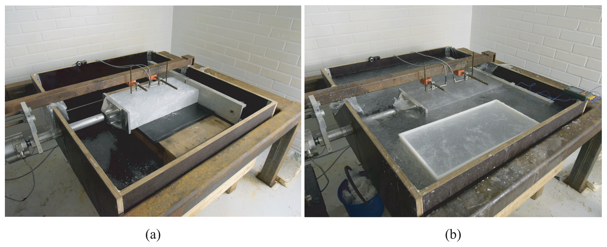
Figure 2 Equipment used in the (a) dry and (b) floating-ice experiments. One of the plastic molds used when growing ice is shown in (b). The thin ice cover of the basin, seen in (b), was broken before performing the experiments.

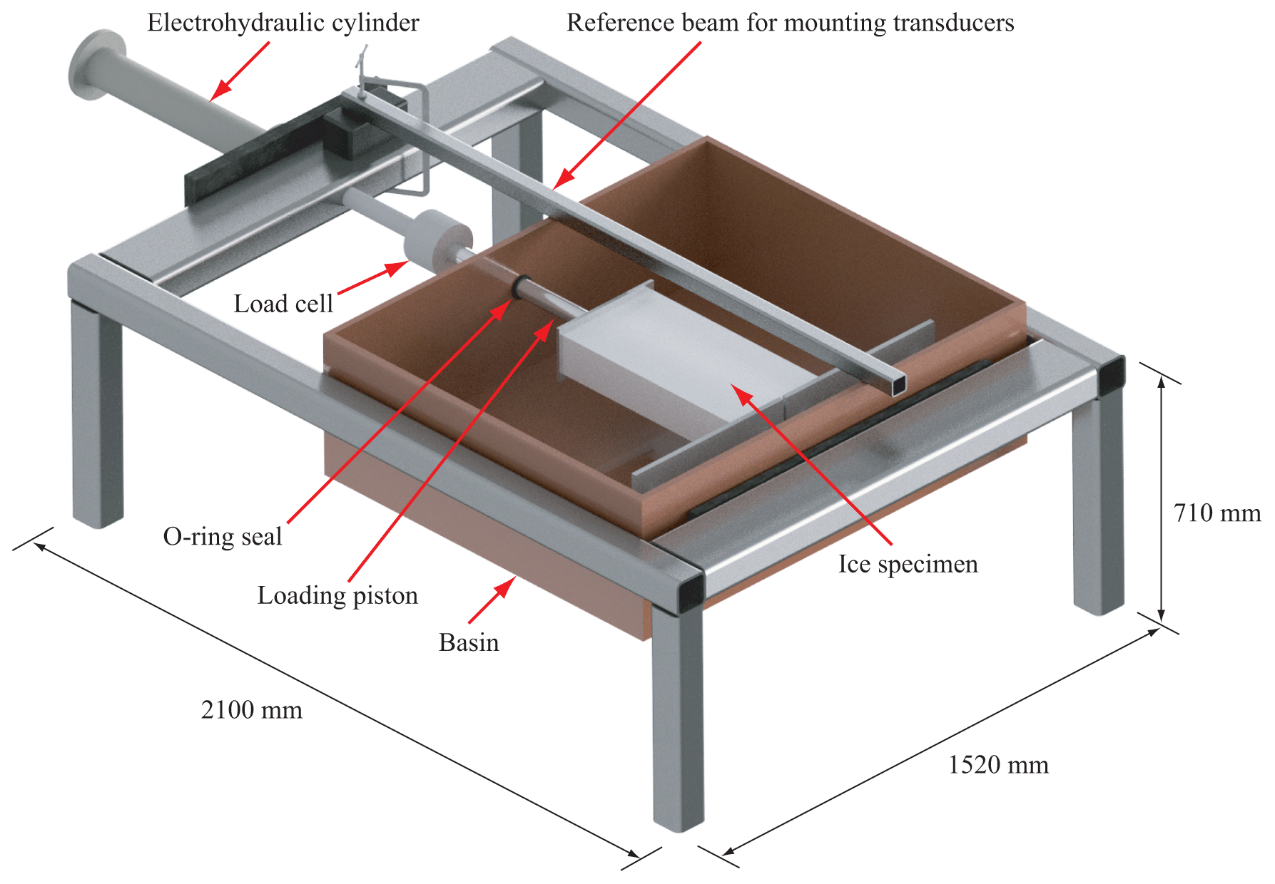
Figure 3 A sketch of the test rig used in the experiments. The inner dimensions of the basin are $\mathrm{1320}\mathrm{mm}\times \mathrm{1280}\mathrm{mm}\times \mathrm{400}\mathrm{mm}$.

The specimens used in the dry experiments (Figs. 2a and 3) were sealed in plastic bags and stored in a freezer at −10 ^∘C for 1–2 d before testing. However, for the floating-ice experiments (see Fig. 2b), the specimens were ejected from the molds, placed in plastic bags with water from the growth tank and quickly transferred to the test basin to minimize brine drainage during the transfer.

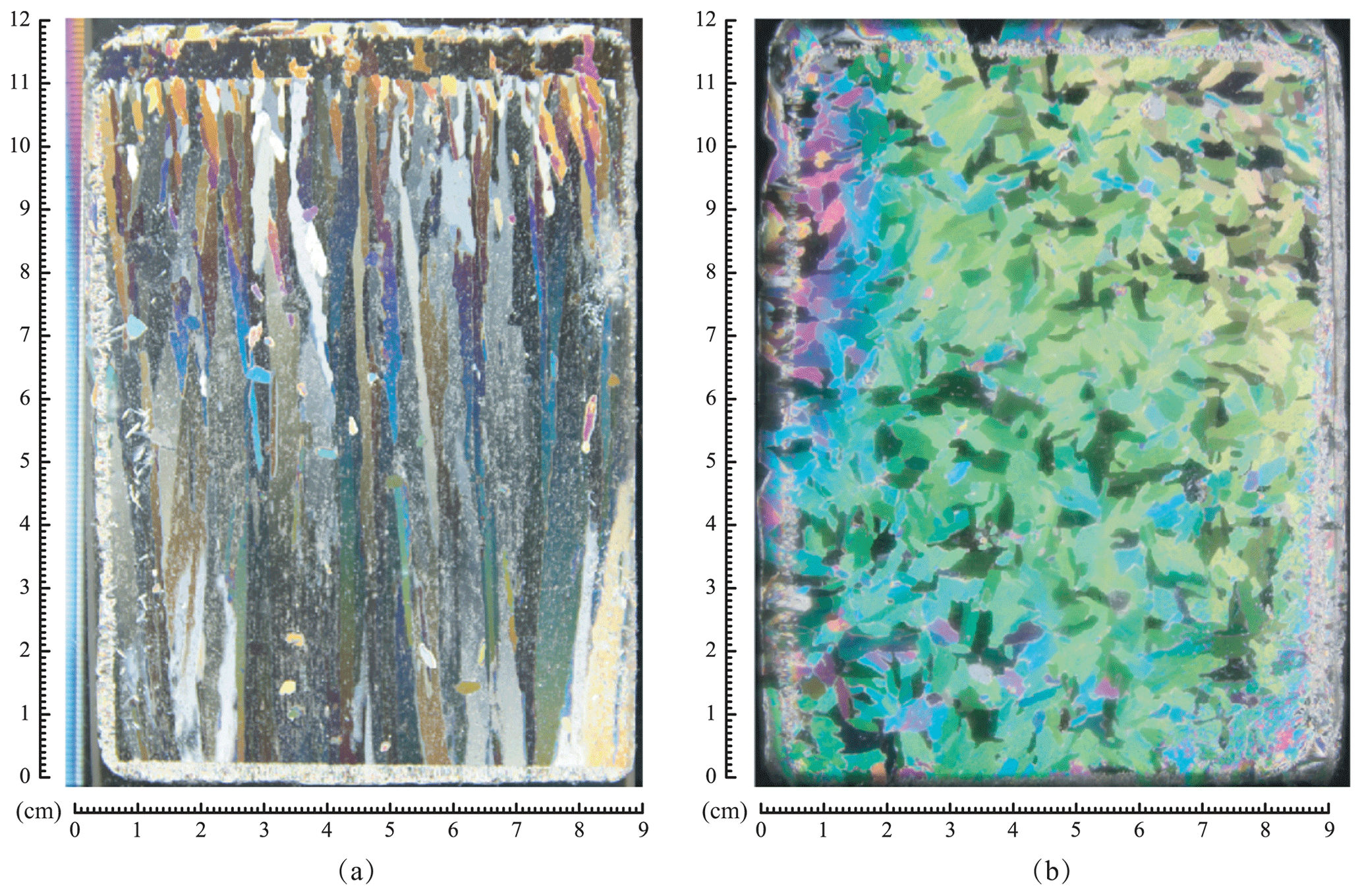
Figure 4 One set of thin sections of the ice (salinity: 5 ppt) grown in this experimental campaign: (a) vertical, (b) horizontal.

Before the experiments, the columnar microstructure of the ice was verified by producing and inspecting thin sections as detailed by Langway (1958). Of special interest was the microstructure close to the specimen boundaries since such molds are somewhat uncommon in ice specimen preparation. Figure 4 shows two typical thin sections from near the boundary of a specimen produced using 24 ppt saline water; one is for the vertical and the other for the horizontal direction as indicated. Figure 4a shows the columnar structure of the ice. The horizontal view in Fig. 4b provides a way to estimate the average grain size by dividing the section area by the number of grains; the average grain size was ≈3.5 mm. The Schmidt equal area net pole projection for one of the thin sections shown in Fig. 5 confirms that the c axes were unaligned in the horizontal plane, as intended.

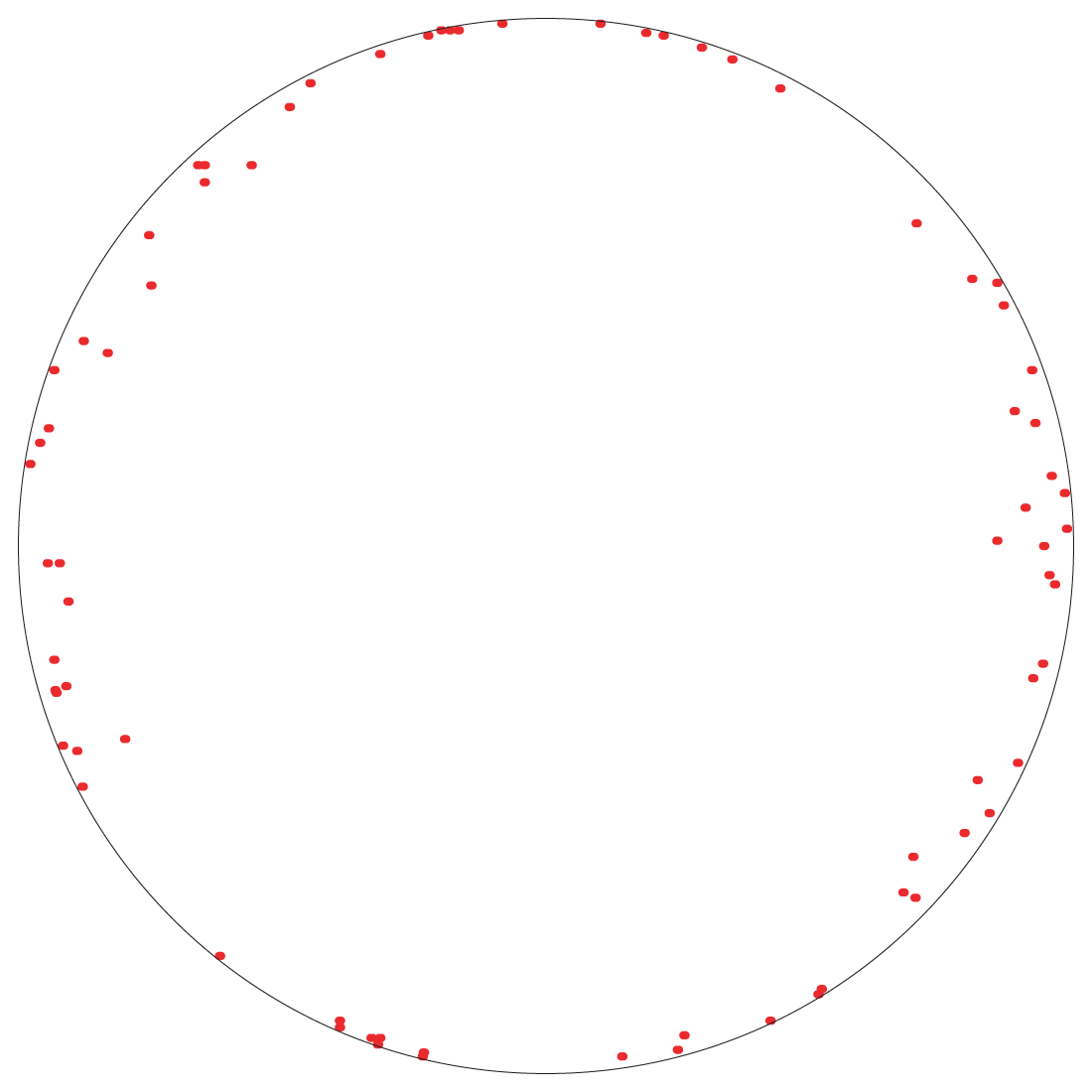
Figure 5 A typical Schmidt equal area net pole projection drawn on the basis of grain orientations.

2.2 Equipment, test matrix and experimental procedure

The experiments were conducted in the same cold chamber used for the saline-ice production. As Figs. 2 and 3 illustrate, an externally mounted electrohydraulic cylinder applied loads to the specimens. The piston passed through a sealed port in the side of the test tank. The piston had a maximum stroke of 800 mm and a loading capacity of 100 kN for compression and 60 kN for tension. The load cell had an accuracy of ±5 N, which is sufficient for all stress levels and cycles of the experiments here. The test basin was constructed of waterproof plywood. The system employed a camera for remote monitoring of the experiments, a three-channel temperature data logger to record the temperature profile of floating ice during testing, a data acquisition processor (DAP) board (model: Data Translation DT9834) and fixtures for arranging displacement sensors to the ice specimens. The temperature data logger had a maximum sampling rate of one datum per 5 s; its measurement range was from −100 to 1300 ^∘C, and it had an accuracy of ±0.5 ^∘C. The DAP board could achieve a maximum scan rate of 500 000 samples per second.

The loading system has a self-equilibrating geometry in that the compressive force applied by the electrohydraulic piston and transmitted through the specimen is balanced by a tensile force in the external load frame (Fig. 3). Care was taken to center the loading piston and the reaction plates on the vertical dimension of the load frame.

The ice deformation was measured as follows. Before the test, two holes were drilled into the specimen. Two iron rods with a cross section of 5 mm×5 mm were then inserted into the holes and frozen in place using a small quantity of cold fresh water. The relative displacement of the rods was monitored by two linear variable differential transformer transducers (LVDTs; model: HBM WA2, with a measurement range and accuracy of 2 and ±0.001 mm, respectively). This relative displacement was used to determine the strain response of the specimen. As shown in Figs. 2 and 3, the LVDTs were mounted on a rectangular piece of steel placed across the basin.

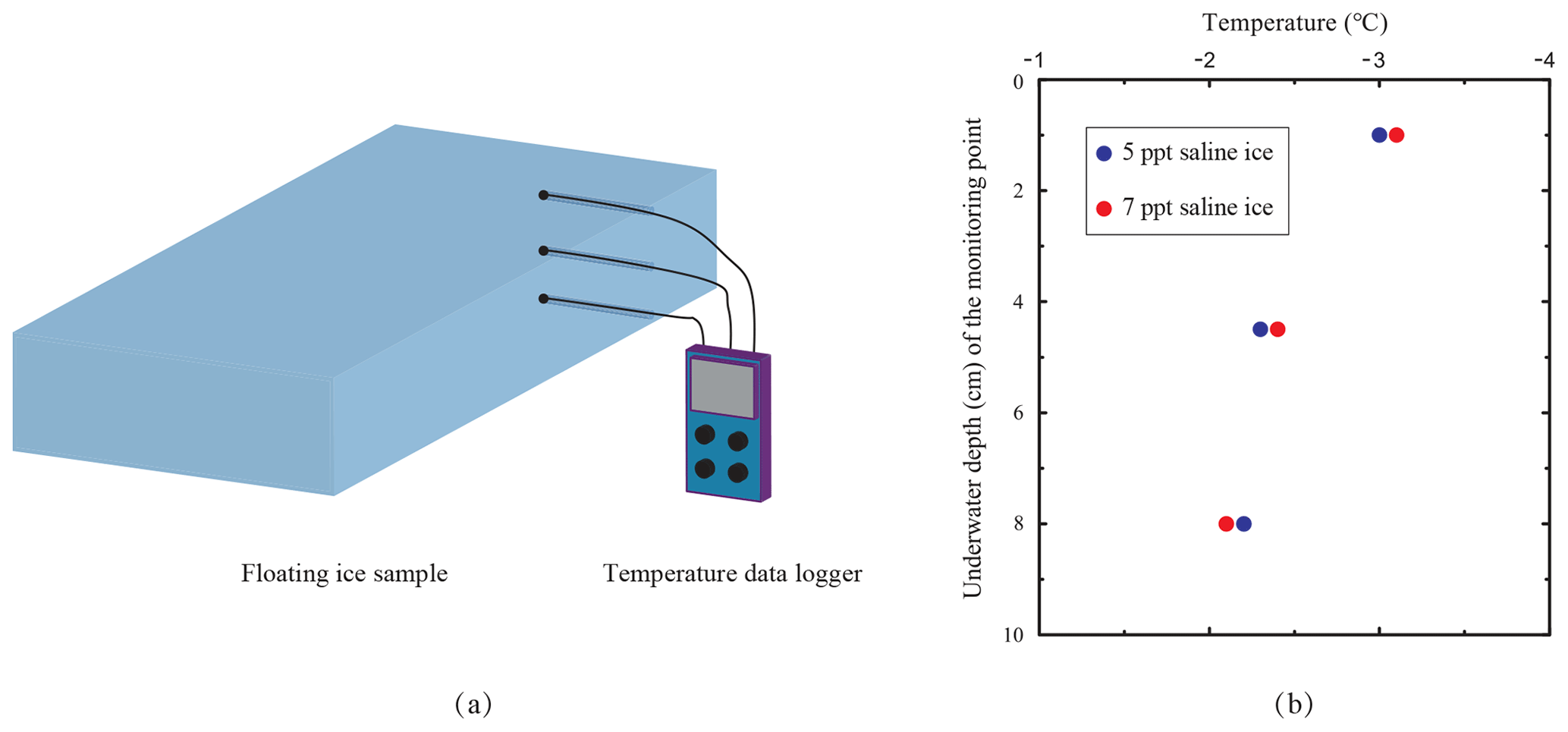
Figure 6 Monitoring of the through-thickness thermal gradient of floating ice: (a) a schematic diagram of the arrangement of the temperature probes and (b) the measured through-thickness thermal gradient inside two floating-ice specimens.

The air temperature was kept at −10 ^∘C during all testing. To measure the through-thickness temperature gradient in all of the floating-ice experiments, temperature probes were frozen into three 2.5 mm diameter, 50 mm deep holes that were drilled on one side face of the specimen. As shown in a sketch in Fig. 6a, one measurement point was in the middle of the specimen from the vertical direction, and the other two were 1.5 mm away from the upper and lower surfaces of the specimen, respectively. During each floating-ice experiment, temperature readings from all three channels remained constant for the duration of the experiment, indicating that the thermal gradient was unaffected by the cyclic loading.

Figure 6b presents typical temperature profiles measured in two floating-ice specimens. For the 5 ppt saline floating ice, the temperature near the top surface, in the middle and near the bottom surface of the specimen was measured to be −3.0, −2.3 and −2.2 ^∘C, respectively, while the values were −3.1, −2.4 and −2.1 ^∘C, respectively, for the 7 ppt saline ice floe. These temperature readings suggest that the average temperature of the floating ice was −2.5 ^∘C, much higher than the air temperature of the cold chamber (−10 ^∘C). The water temperature at 5 cm below the water surface was measured to be $\approx -\mathrm{1.8}$ ^∘C in the floating-ice tests.

Table 1 The test matrix of this experimental campaign. The campaign included two test types, two ice salinities, six periods and two test-type-dependent load levels. For each case, two specimens harvested from two ice sheets were tested.

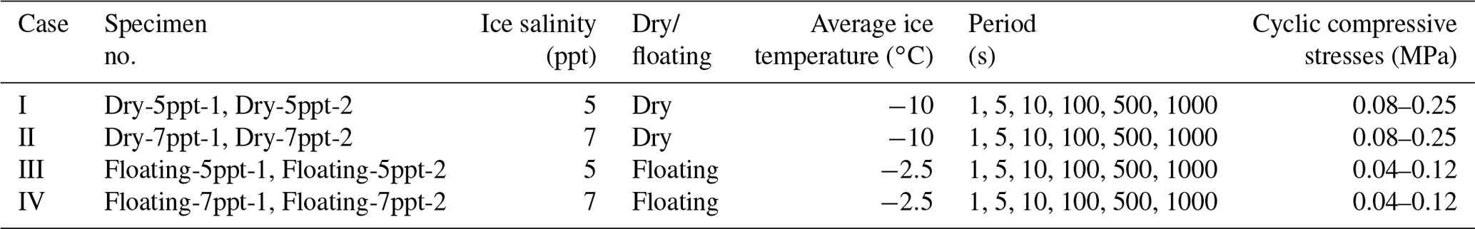
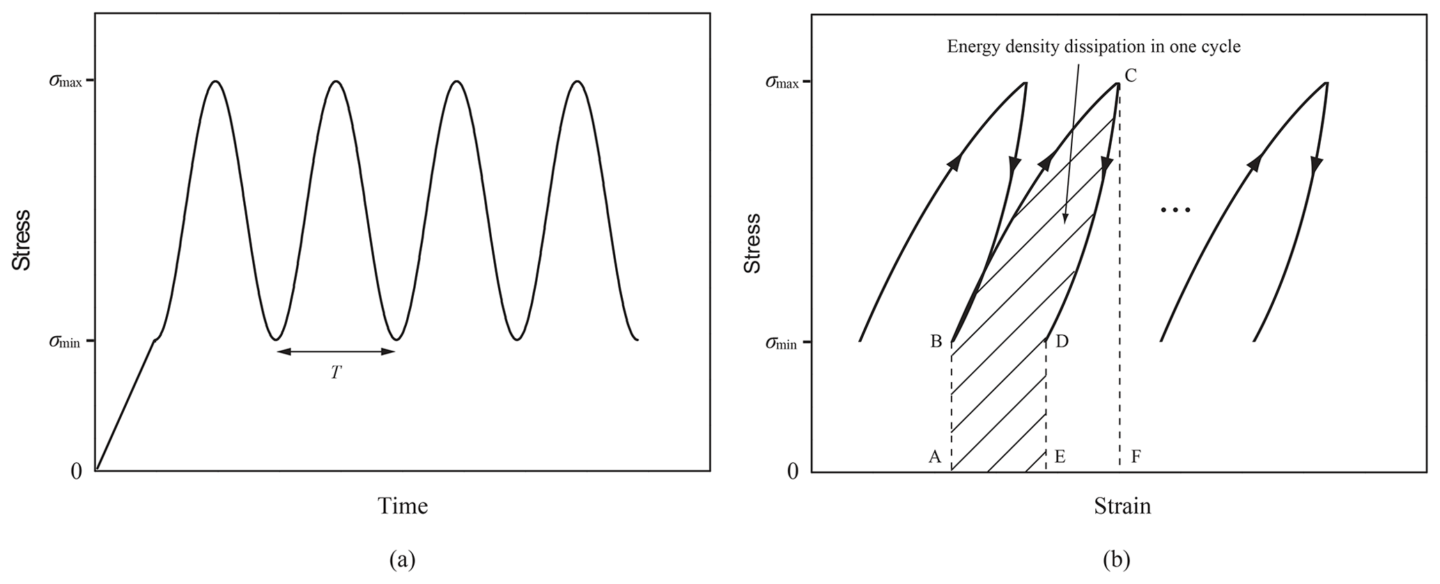
Figure 7 Schematic diagrams of the cyclic loads: (a) the inputted stress waveform and (b) the method for calculating the energy density dissipated in one loading cycle (in other words, region ABCDE).

The test matrix called for applying relatively low cyclic compressive stress levels with the system in load control. Figure 7 presents the loading waveforms used in the experiments, and the test matrix is given in Table 1. In the experiments, the ice was first loaded with a linear ramp to reach an initial compressive stress level, at which point a compressive haversine waveform was immediately applied. In Fig. 7a, σ_max and σ_min represent the upper and the lower bounds of the cyclic compressive stress, respectively, and T denotes the period for one loading cycle. As indicated by Table 1, six periods ranging from 1 to 10³ s were employed; these periods cover the main range of ocean wave periods, which usually vary from several seconds to tens of seconds (Reistad et al., 2011; Zijlema et al., 2012). In each dry test, only a fixed frequency was applied. Once the test was completed, the specimen recovered for 15 min before subsequent load cycles were applied. For all dry tests, the duration of the initial loading ramp was fixed to be 1 s. In each of the tests corresponding to T=1, 5, 10 and 100 s, 18 cycles were applied (N=18), while for those with T=500 and 1000 s, N equaled 9 and 4, respectively. The sequence of loading cycles was in ascending order of T in all cases. As a time-saving measure and to avoid freezing of the open water in the basin, cyclic stresses with increasing periods were applied continuously in the floating-ice tests. The number of cycles for each period was as follows: for T=1, 5 or 10 s, N equals 10; for T=100 s, N equals 2; and for T=500 or 1000 s, N equals 1.

The cyclic compressive stress applied to the dry specimens varied from 0.08 to 0.25 MPa, which could be justifiably expected to not lead to severe damage of the specimen while being high enough to generate measurable strain (Cole and Dempsey, 2001). The stress in the floating experiments was lower, varying from 0.04 to 0.12 MPa, to avoid damage. For each case listed in Table 1, two specimens harvested from two ice sheets were subjected to each set of conditions. The specimens were named according to their salinity, test conditions (dry/floating), and the ice sheet from which they originated. For example, specimen name Dry-5ppt-1 indicates that it came from the first 5 ppt saline ice sheet and was tested under dry, isothermal conditions.

Figure 7b illustrates how the energy dissipation in the cyclic loading experiments was calculated. For common engineering materials subjected to uniaxial cyclic compression, the strain along the compressive direction versus the stress is usually characterized by hysteresis loops. The strain energy density dissipated in a loading cycle can be determined by integrating the stress–strain curve. As shown in Fig. 7b, the area under the loading curve (region ABCF) represents the maximum strain energy input via the testing machine during a load cycle, and the area under region CDEF denotes the strain energy released during the unloading portion of the cycle. The energy density dissipation (EDD) in one full loading–unloading cycle is given by the difference between the areas of regions ABCF and CDEF (Liu et al., 2017, 2018). The energy density consumed in the hysteresis loop can, in general, be attributed to the internal friction and, in some cases, damage to the material. For each cycle, the energy dissipation rate (EDR) can be defined as the ratio of the dissipated energy to the input energy, namely the area of the region ABCDE divided by that of the region ABCF.

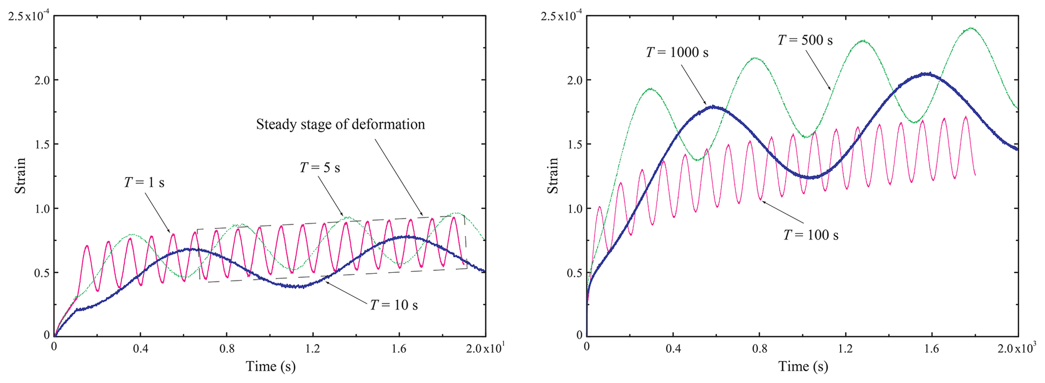
Figure 8 Strain-time curves of specimen Dry-5ppt-1 tested with stresses varying from 0.08 to 0.25 MPa and with a temperature of −10 ^∘C.

3 Experimental results

Figure 8 presents strain-time plots obtained from the dry experiments using specimen Dry-5ppt-1 under the indicated conditions. The strain-time curves manifest the following feature: if a line were drawn through the maximum value for each cycle, the slope of the line would first decrease from its initial value for some number of cycles and then settle down to an almost-constant value. This observation means that the strain response of the ice specimen under sinusoidal compressive stress reaches a relatively steady stage after the initial transient of the anelastic strain is exhausted and that in this steady stage the accumulated viscous or permanent strain increases linearly with time. In addition, Fig. 8 shows that the longer the period T of cyclic loading, the larger the strain amplitude in one steady-stage cycle. The total amount of strain does not strictly increase with the loading period. This may be because the loading platen and the specimen did not always achieve perfect contact immediately, causing some error in the strain measured in this initial stage of loading. Once intimate contact was achieved, the measured strain became reliable.

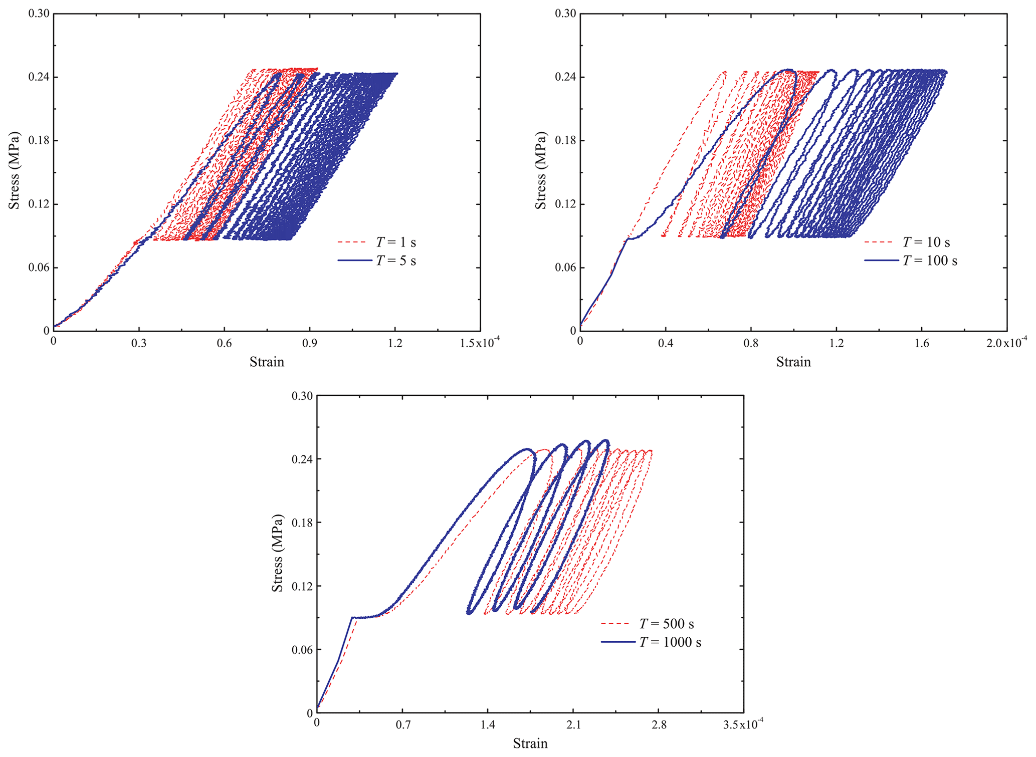
Figure 9 Stress–strain curves of specimen Dry-5ppt-1 tested with stresses varying from 0.08 to 0.25 MPa and with a temperature of −10 ^∘C.

Figure 9 shows the stress–strain curves for the same experiments. In each case, the area of the hysteresis loop for the first few cycles was comparatively large and then gradually decreased to a constant value as the specimen reached the steady deformation stage described in the previous paragraph. For example, the hysteresis loops after the first stress cycle in the dry experiment with T=1000 s are similar; N=4 is enough for the dry specimen at T=1000 s to show steady-state response. Thus, the EDD (Fig. 7b) decreases from its initial value to an approximately constant value. It is clear that the steady-state hysteresis loop area increases with the period of the cyclic loading, consistent with earlier studies (Cole, 1990; Murdza et al., 2018; Weber and Nixon, 1996).

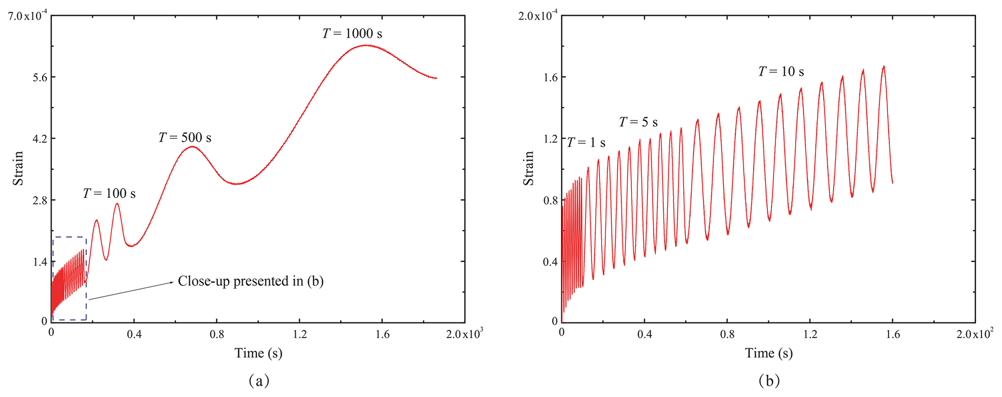
Figure 10 Strain response of specimen Floating-5ppt-1 tested with stresses varying from 0.04 to 0.12 MPa and with an average temperature of −2.5 ^∘C: (a) shows the response for all periods, T, of cyclic loading, while (b) presents a close-up showing the cycles for T=1, 5 and 10 s.

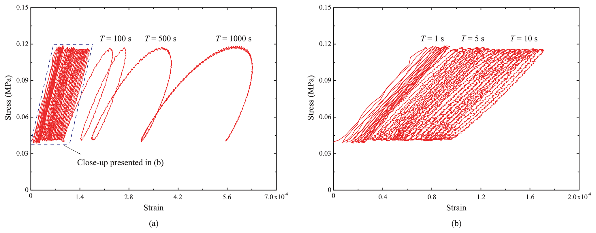
Figure 11 Stress–strain plots of specimen Floating-5ppt-1 tested with stresses varying from 0.04 to 0.12 MPa and with an average temperature of −2.5 ^∘C: (a) shows the response for all periods, T, of cyclic loading, while (b) presents a close-up showing the cycles for T=1, 5 and 10 s.

Table 2 The energy density (J m⁻³) dissipated in a typical loading–unloading cycle of each experiment.

Figures 10 and 11 display a set of strain-time plots and the corresponding stress–strain curves for the floating-ice experiments on the 5 ppt saline ice specimens, respectively. The curves in these two figures show similar features to those in Figs. 8 and 9 for dry experiments. The floating ice also reached a steady state of deformation after some loading cycles, and the amplitude of the steady-state strain response still increased with T. Similar to the results of the dry experiments, Fig. 11 indicates that the longer the loading period, the larger the strain increment of the floating specimen under one steady-state loading–unloading cycle. Comparison of Figs. 9 and 11 in the steady state shows that, for constant T, both the strain increment per cycle and the area of one hysteresis loop, are larger in the floating-ice experiments than in the dry experiments even though the stress levels are lower than in the dry experiments. It is thus evident that the decreased stress levels in the floating-ice experiments did not fully compensate for the temperature effects on the viscous and viscoelastic components of strain as, for example, the viscous strain rate of a floating 5 ppt saline ice specimen is 14 times that of the corresponding dry specimen.

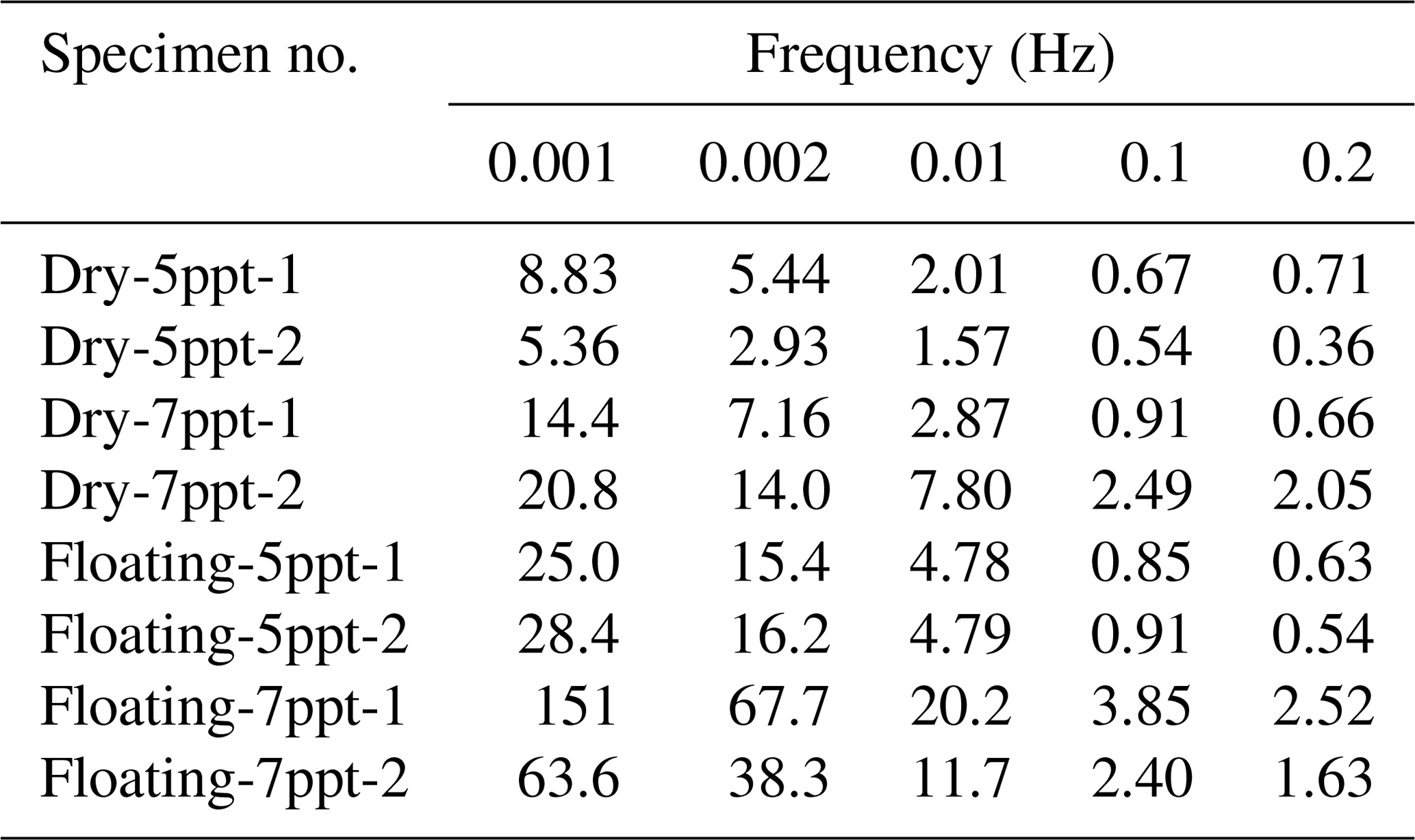
Table 3 The energy dissipation rate (%) in a typical loading–unloading cycle of each experiment.

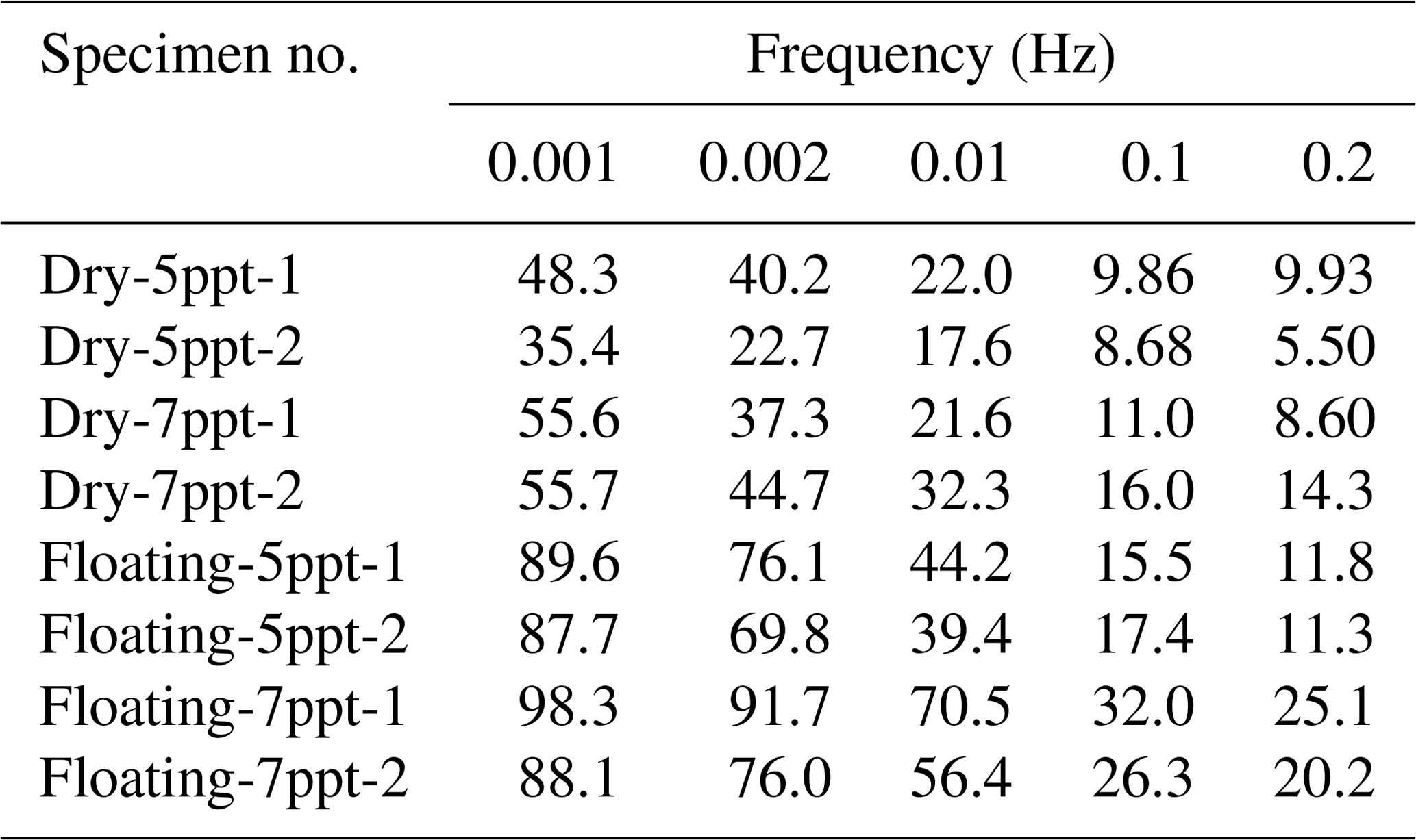
The energy density dissipation (EDD) and the energy dissipation rate (EDR) per cycle during steady-stage deformation (Sect. 2.2 and Fig. 7b) allow quantitative comparisons of the inelastic behavior of specimens as a function of test conditions. These are presented in Tables 2 and 3 for all experiments except the 1 s period experiment, for which the hysteresis loop areas are too small for accurate measurements. Tables 2 and 3 indicate that both the EDD and the EDR decrease with the increase in loading frequency. Moreover, under the same frequency, the 7 ppt saline ice has larger EDD and EDR values than the 5 ppt saline ice irrespective of the experiment type. In addition, the floating-ice experiments always exhibit higher EDD and EDR values than the dry experiments regardless of the ice salinities. The differences in the values of EDD are especially significant for low frequencies. For example, in the experiments with T=1000 s, the average value of EDD for the 5 ppt saline dry specimens is only 24 % of that of the 5 ppt saline floating specimens and 44 % of that of the 7 ppt saline dry specimens. However, for the experiments with T=5 s, the average value of EDD in the former case is 47 % and 77 % of that in the latter two cases, respectively. Thus, the ice salinity and the test conditions have a more significant influence on the energy dissipation of the ice when the cyclic loading period is long.

4 Material modeling

The hysteresis loops of the stress–strain curves manifest viscous and anelastic properties of the ice. According to previous studies (Cole, 1995; Leclair et al., 1999), in low-stress cyclic loading experiments, the microstructure of the ice remains unaffected by loading, or in other words, no damage occurs within the material. In the present case of polycrystalline ice, the anelastic deformation is mainly attributed to two relaxation mechanisms: lattice dislocation relaxation and grain boundary sliding. Viscous straining is attributable to basal dislocation. In this section, a dislocation-based model (Cole, 1995; Cole and Durell, 2001), which accounts for these mechanisms, is used to predict the strain response of the ice specimens based on their physical properties and experimental conditions. Here the model is only briefly described, but a detailed description can be found from Cole et al. (1998), where the model is also demonstrated to reproduce the viscous and anelastic behavior of dry specimens. Here the applicability of the model in predicting the behavior of floating laboratory-prepared ice specimens subjected to cyclic loading is tested for the first time.

4.1 Brief description of the model

In the physically based model by Cole (1995) and Cole and Durell (2001), the axial strain, ε, of ice under uniaxial cyclic compression is considered to be composed of elastic, anelastic (delayed elastic) and viscous components, denoted here as ε_e, ε_a and ε_v, respectively. The axial strain is expressed as

$$\begin{array}{}\text{(1)}& \mathit{\epsilon }={\mathit{\epsilon }}_{\mathrm{e}}+{\mathit{\epsilon }}_{\mathrm{a}}+{\mathit{\epsilon }}_{\mathrm{v}}.\end{array}$$

In the case of sinusoidal stress waveform, ε_e can be written as

$$\begin{array}{}\text{(2)}& {\mathit{\epsilon }}_{\mathrm{e}}={\displaystyle \frac{\mathit{\sigma }\left(\mathit{\omega },t\right)}{E_{\mathrm{0}}}},\end{array}$$

where ω is the angular frequency of the stress waveform, and E₀ is the unrelaxed modulus. Although detailed expressions have been developed for the effective elastic modulus as a function of crystallography, brine and gas porosity, and temperature, a simplified approach is adopted in the present effort. The anelastic component ε_a incorporates both above-mentioned relaxation mechanisms to represent the time-dependent recoverable deformation. For the steady-stage deformation, ε_a of ice subjected to sinusoidal compressive stress can be decomposed as (Cole and Dempsey, 2001)

$$\begin{array}{}\text{(3)}& {\mathit{\epsilon }}_{\mathrm{a}}=\mathit{\sigma }\left(\mathit{\omega },t\right)\left[D_{\mathrm{1}}^{\mathrm{d}}\left(\mathit{\omega }\right)+D_{\mathrm{2}}^{\mathrm{d}}\left(\mathit{\omega }\right)+D_{\mathrm{1}}^{\mathrm{gb}}\left(\mathit{\omega }\right)+D_{\mathrm{2}}^{\mathrm{gb}}\left(\mathit{\omega }\right)\right],\end{array}$$

where the compliance terms, D, with the superscripts “d” and “gb” denote the compliances induced by dislocation and grain boundary sliding, respectively. The compliance terms are defined as (Cole et al., 1998)

$$\begin{array}{}\text{(4)}& {\displaystyle }{D}_{\mathrm{1}}^{\mathrm{d}}\left(\mathit{\omega }\right)=\mathit{\delta }{D}^{\mathrm{d}}\left\{\mathrm{1}-{\displaystyle \frac{\mathrm{2}}{\mathit{\pi }}}{\tan }^{-\mathrm{1}}\left[e^{\left({\mathit{\alpha }}^{\mathrm{d}}{s}^{\mathrm{d}}\right)}\right]\right\}\text{(5)}& {\displaystyle }{D}_{\mathrm{1}}^{\mathrm{gb}}\left(\mathit{\omega }\right)=\mathit{\delta }{D}^{\mathrm{gb}}\left\{\mathrm{1}-{\displaystyle \frac{\mathrm{2}}{\mathit{\pi }}}{\tan }^{-\mathrm{1}}\left[e^{\left({\mathit{\alpha }}^{\mathrm{gb}}{s}^{\mathrm{gb}}\right)}\right]\right\}\text{(6)}& {\displaystyle }{D}_{\mathrm{2}}^{\mathrm{d}}\left(\mathit{\omega }\right)={\mathit{\alpha }}^{\mathrm{d}}\cdot \mathit{\delta }{D}^{\mathrm{d}}{\displaystyle \frac{\mathrm{1}}{e^{\left({\mathit{\alpha }}^{\mathrm{d}}{s}^{\mathrm{d}}\right)}+e^{\left(-{\mathit{\alpha }}^{\mathrm{d}}{s}^{\mathrm{d}}\right)}}}\text{(7)}& {\displaystyle }{D}_{\mathrm{2}}^{\mathrm{gb}}\left(\mathit{\omega }\right)={\mathit{\alpha }}^{\mathrm{gb}}\cdot \mathit{\delta }{D}^{\mathrm{gb}}{\displaystyle \frac{\mathrm{1}}{e^{\left({\mathit{\alpha }}^{\mathrm{gb}}{s}^{\mathrm{gb}}\right)}+e^{\left(-{\mathit{\alpha }}^{\mathrm{gb}}{s}^{\mathrm{gb}}\right)}}},\end{array}$$

where S^d=ln (τ^dω); τ^d is the central relaxation time (Cole and Durell, 1995). The term α is a so-called peak-broadening term, which accounts for the effect of a distribution in relaxation times of the basal-plane dislocations. The grain boundary relaxation is calculated using similar mathematic expressions as the dislocation relaxation but has a different strength, activation energy and peak-broadening term. The activation energy is 1.32 eV for the grain boundary relaxation and 0.55 eV for the dislocation relaxation (Cole and Dempsey, 2001). The peak-broadening terms for lattice dislocation relaxation and grain boundary sliding relaxation are typically ≈0.5 and 0.6, respectively, determined experimentally by Cole (1995) and Cole and Dempsey (2001) and also validated by Heijkoop et al. (2018). The strength of the dislocation relaxation is calculated from

$$\begin{array}{}\text{(8)}& \mathit{\delta }{D}^{\mathrm{d}}={\displaystyle \frac{\mathit{\rho }\mathrm{\Omega }{b}^{\mathrm{2}}}{K}},\end{array}$$

where b represents the magnitude of Burgers vector ($b=\mathrm{4.52}\times {\mathrm{10}}^{-\mathrm{10}}$ m); ρ denotes the mobile dislocation density, often found to be on the order of 10⁹ m⁻²; Ω is an orientation factor, determining the average basal-plane shear stress induced by the background normal stress ($\mathrm{\Omega }=\mathrm{1}/\mathit{\pi }\approx \mathrm{0.32}$ for a horizontal specimen made of unaligned columnar ice; Cole, 1995); K is a restoring stress constant, determined as 0.07 kPa for polycrystalline ice in experiments (Cole and Durell, 2001).

In Eq. (1), the viscous strain ε_v is often estimated with the following formulae (Cole and Durell, 2001):

$$\begin{array}{}\text{(9)}& {\displaystyle }{\mathit{\epsilon }}_{\mathrm{v}}=\underset{\mathrm{0}}{\overset{t}{\int }}{\dot{\mathit{\epsilon }}}_{\mathrm{v}}d\stackrel{\mathrm{‾}}{t}\text{(10)}& {\displaystyle }{\dot{\mathit{\epsilon }}}_{\mathrm{v}}={\displaystyle \frac{\mathit{\beta }\mathit{\rho }{\mathrm{\Omega }}^{\mathrm{1.5}}{b}^{\mathrm{2}}{\mathit{\sigma }}_{\mathrm{creep}}}{B_{\mathrm{0}}}}{e}^{\left(-\frac{Q_{\mathrm{glide}}}{k{T}^{\ast }}\right)},\end{array}$$

where β equals 0.3, Q_glide equals 0.55 eV, and B₀ equals $\mathrm{1.205}\times {\mathrm{10}}^{-\mathrm{9}}$ Pa s. The term k is Boltzmann's constant; T^∗ is the temperature in kelvin. By using the above definitions and equations, the strain of the ice specimen can be finally determined via Eq. (1).

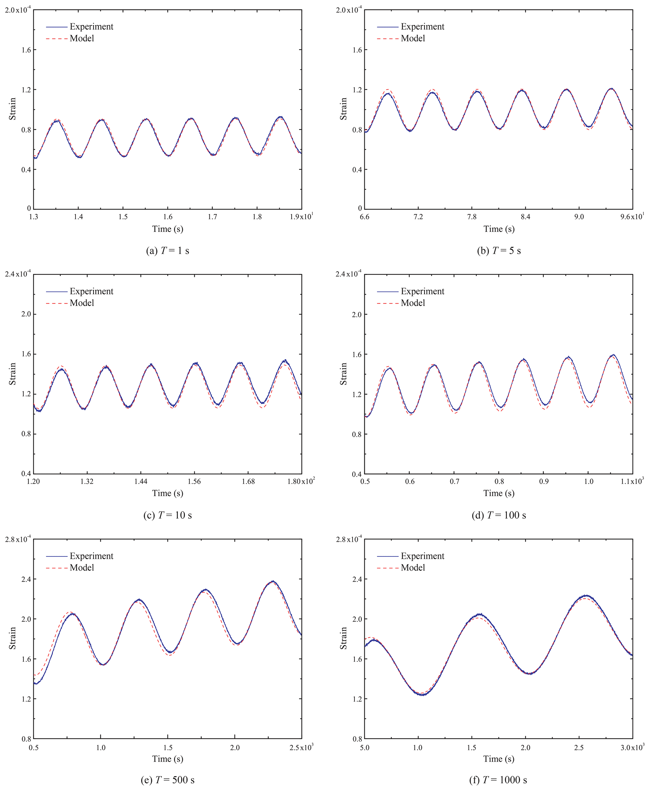
Figure 12 Comparison between the experimentally measured strain-time curves (in the steady stage) and the results yielded by the physically based model for specimen Dry-5ppt-1, tested with stresses varying from 0.08 to 0.25 MPa and with a temperature of −10 ^∘C.

4.2 Modeling

In this study, the key quantity to be determined from the experiments is the dislocation density (ρ). With knowledge of the microstructure and orientation factor (Ω) and given the experimental conditions, the anelastic term δD^d and the viscous strain rate can be calculated directly. We opt here to determine E₀ empirically. This was done by trial and error until the stress–strain curves generated by the model matched with those measured in the experiments with T=10, 100 and 500 s. By making the slopes of the modeled and experimental hysteresis loops for T=10 s comparable, E₀ could be determined. This is because the behavior of the specimens is mainly dominated by the unrelaxed modulus E₀ when the loading frequency is high (here 0.1 to 1 Hz), as indicated in Figs. 9 and 11. From Eqs. (9) and (10), one can find that the strain increment under one loading cycle is dependent on the dislocation density ρ; based on this, the dislocation density ρ was estimated by using the experimental results of T=100 and 500 s, and δD^d was then determined from Eq. (8). δD^gb was determined by referring to previous work (Cole, 1995) because the grain boundary relaxation strength could be reasonably assumed constant for the ice material of interest here, and its effect on inelastic behavior of ice was significantly less than the dislocation mechanism. The values determined for the parameters are tabulated in Table 4. Subsequently, the model based on these parameter values was applied to predict the test results for other loading periods. An example of the comparison of experimental and modeling results is presented in Fig. 12, in which the steady-state strain curves from all dry experiments on the 5 ppt saline ice specimen are accompanied by the simulated ones.

Table 4 Values of the model parameters calibrated for simulating the strain response of the ice specimens (in Sect. 5, these values are discussed and compared to those reported in the references).

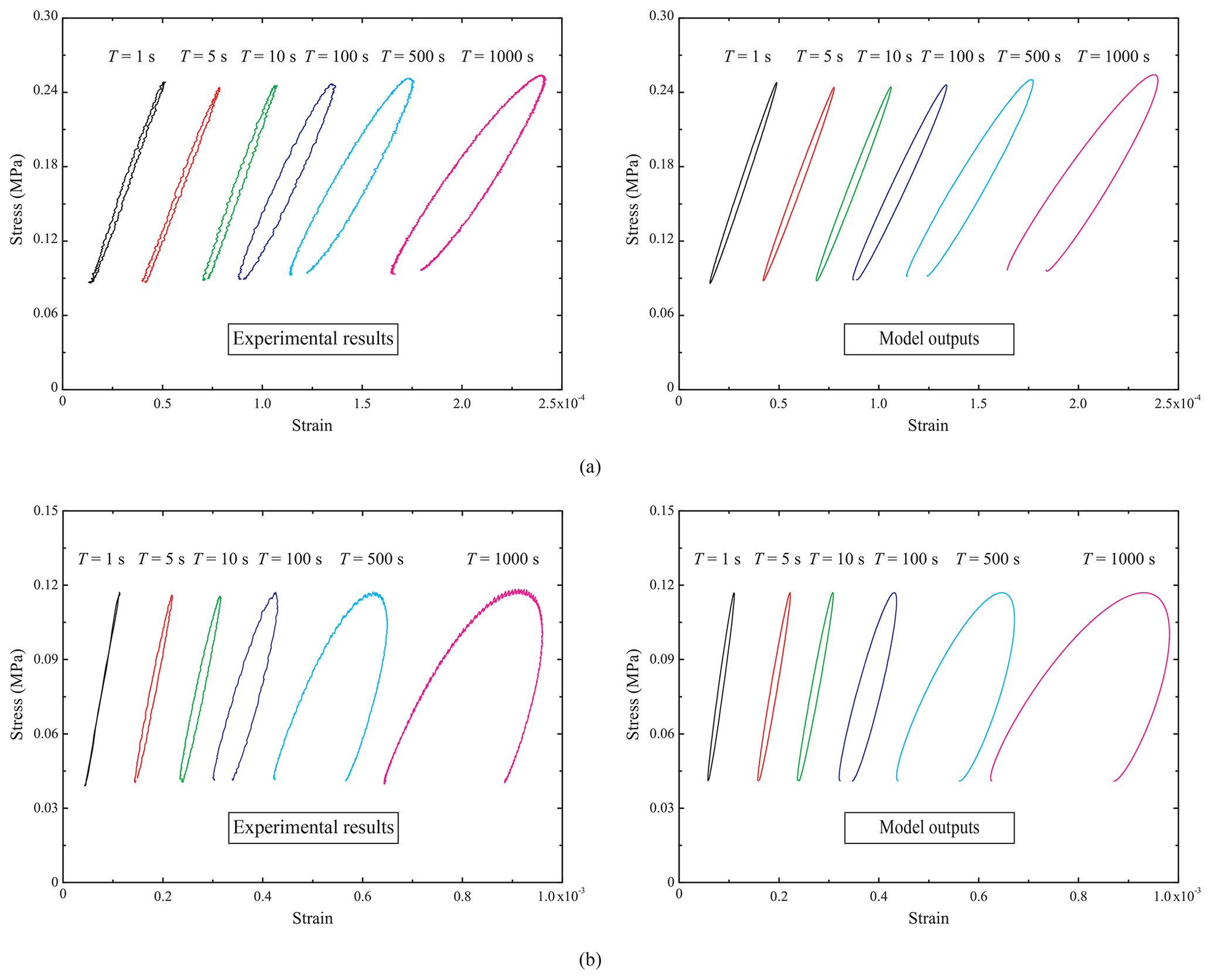
Figure 13 Comparison between the steady-state stress–strain hysteresis loop measured in the experiments and that outputted from the model for (a) specimen Dry-5ppt-1 with a temperature of −10 ^∘C and (b) specimen Floating-5ppt-1 with an average temperature of −2.5 ^∘C (note that, to compare the representative hysteresis loops in all the different-frequency experiments with those outputted by the model in a more concise and intuitive way, the prestrains before the hysteresis loops drawn here are not equal to the experimental values).

Figure 12 shows that the modeled strain records compare well with those from the experiments with period T=1, 5 and 1000 s. The model reproduced the steady-state strain response of the specimens very well for all tested frequencies. Figure 13 presents the stress–strain hysteresis loops from the same experiments together with those produced by the model. The hysteresis loops generated by using the model are very similar to those from the experiments. The loop area increases with T in both the experiments and simulations.

Table 5 Modeling results of the strain energy density (J m⁻³) dissipated per loading–unloading cycle (the values given in parentheses are error percentages of model predictions relative to experimental results).

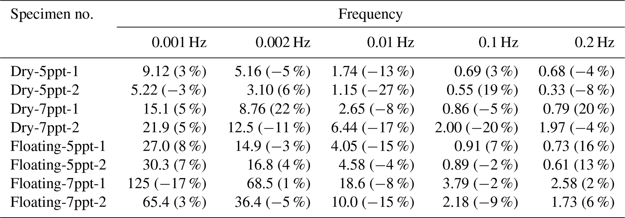
Table 6 Modeling results of the strain energy dissipation rate (%) per loading–unloading cycle (the values given in parentheses are error percentages of model predictions relative to experimental results).

For assessing the model in more detail, the values of EDD and EDR derived using it are given in Tables 5 and 6, respectively, and moreover compared with the data from all the experiments (the test matrix is given in Table 1). Tables 5 and 6 indicate that the model predicts the values of EDD and EDR well for all cyclic loading periods studied here. In general, the error in the predicted EDD and EDR values is within 20 %, with the exception of only few cases. No obvious trend between the magnitude of error and loading period or experiment type was observed. Note that for a given ice specimen, one dislocation density value adequately models the steady-state strain responses and energy dissipation values in tests conducted with different frequencies. The value of dislocation density thus remained constant through the cyclic loading.

4.3 Further validation

The above results show that the model can yield satisfactory predictions of the viscous and anelastic behavior of both dry and floating specimens. One may argue that the good agreement between the model predictions and the experimental results only indicates the capability of the model to predict the results for the experiments with the same stress levels as those used to calibrate the model parameters. To check whether the model can predict the results of the experiments with different stress levels than those above, additional experiments were performed on specimen Dry-5ppt-1 with higher stress (0.1–0.3 MPa) and on specimen Floating-7ppt-1 with lower stress (0.005–0.085 MPa; nominal cyclic stress of 0.005–0.085 MPa is low, but the setup could achieve it: with the accuracy of the system, the actual stress applied to the specimen was 0.005 (±0.001)–0.085 (±0.003) MPa). The model was then used to determine the strain response and energy dissipation in these tests using the parameterization based on the experiments of Sect. 3 (Table 4).

Figure 14 Comparison between the steady-state stress–strain hysteresis loops measured in the experiments and those predicted by the dislocation-based model for (a) specimen Dry-5ppt-1, tested with stresses varying from 0.1 to 0.3 MPa and with a temperature of −10 ^∘C, and (b) specimen Floating-5ppt-1, tested with stresses varying from 0.005 to 0.085 MPa and with an average temperature of −2.5 ^∘C (note that, to compare the representative hysteresis loops in all the different-frequency experiments with those outputted by the model in a more concise and intuitive way, the prestrains before the hysteresis loops drawn here are not equal to the experimental values).

Figure 14 compares the stress–strain hysteresis loops obtained in the supplementary experiments with the predictions yielded from the model. Good agreement is observed between the predicted and measured hysteresis loops. Again, the relative errors in the EDD and EDR values are found to be less than 20 % for most data sets. The model is, indeed, capable of predicting the deformation of saline ice in a dry environment or when floating in water irrespective of the stress level (given that the stress levels are moderate and do not cause an increase in dislocation density during deformation). The applicability of the model is highlighted by the fact that once the model parameters are calibrated through benchmark experiments (the elastic modulus and dislocation density in the present case), it yields sound predictions for the experiments conducted with other stress levels.

5 Discussion

Although past laboratory-scale work has provided insight into the mechanical behavior of sea ice, the work has been mostly performed using relatively cold, dry and isothermal specimens. The results above indicate that more attention should be paid to the mechanical behavior of relatively warm floating ice with a naturally occurring temperature gradient. Here efforts were made to develop a relatively low-cost, convenient and useful approach for laboratory-scale floating-ice experiments and for preparing small-scale, saline columnar ice specimens. The thin sections (Figs. 4 and 5) indicated that the measures taken on the ice production guaranteed the generation of nonoriented columnar ice. Moreover, the thin sections showed that the molds used for specimen preparation do not influence the columnar ice microstructure. This is encouraging as molds are not often incorporated into growing sheets of nonoriented columnar ice. The use of molds in this way significantly simplified specimen preparation and resulted in accurate dimensions. The molds are especially effective in the experiments on floating-ice specimens: the specimens produced thus have proper dimensions, require no cutting, have a realistic temperature gradient and can be quickly transferred to the test basin, so brine loss is minimized.

The results above are in qualitative agreement with what would be expected for floating ice as, for example, floating specimens with a through-thickness thermal gradient and a mean temperature of −2.5 ^∘C exhibit lower modulus and more pronounced inelastic deformation in comparison with dry specimens at −10 ^∘C, as would be expected based on full-scale observations of the effect of temperature on this property (Timco and Weeks, 2010; Cole, 2020). This gives confidence on the methods employed in the production and mechanical testing of the specimens. Further, the good agreement between the results for floating ice and the corresponding model predictions shows quantitative validity of the approach taken here. All in all, the results suggest that the chosen experimental techniques (including the loading system, the strain measurement scheme, the data acquisition system and settings) worked well and provided useful results for the analysis. An exception is some of the 1 s period experiments, which yielded strain responses with unexpected features; this is because the hysteresis loop areas are very small in size, making accurate measurements with the used setup challenging. This could be circumvented in future experiments by using techniques and devices with even higher precision and setting a higher sampling rate of data acquisition. The methods proposed in this study to conduct laboratory experiments on floating-ice experiments are practical and can provide a convenient approach for relatively low-cost experimentation on floating ice.

The laboratory work here not only demonstrates the availability of the proposed experimental methods but also contributes to the understanding of the constitutive behavior of ice. A common trend in developing material models is to ensure they have a solid physical basis, that is, that they are based on an understanding of the physical processes that underlie the mechanical phenomena of interest. Above we used one such physically based model introduced by Cole (1995). Earlier work, which has been based on the experiments resembling the dry experiments here, has shown that the model is capable of predicting the inelastic deformation of sea ice via dislocation-based mechanisms and is able to estimate the effective dislocation density in ice from experimental results. Here the model was successfully validated against the results from the floating-ice experiments. Moreover, the results indicated that once the constant dislocation density value of the specimens was determined, the model adequately predicted the steady-stage deformation for the cyclic loading experiments conducted with different frequencies and stress levels. Even if the use of floating specimens could be considered to only address the temperature profiles of in situ floating ice (with some other environmental conditions of natural ice floes ignored), the above results bring confidence to the model and demonstrate its potential in modeling practical applications involving ice in such conditions, especially considering that some research has been launched to devote to a numerical implementation of the model (O'Connor et al., 2020).

The good agreement between the experimental and modeling results also motivates discussion on the parameter values in Table 4. Expectedly, the floating-ice specimens have lower unrelaxed moduli than the dry specimen. For the 5 and 7 ppt saline ice, the average elastic modulus of the floating specimens is 66 % and 55 % lower than that of the dry specimens, respectively. In the dry experiments, the isothermal 7 ppt saline ice has a 31 % lower average elastic modulus than the 5 ppt saline ice. In the floating-ice experiments, the 7 ppt saline specimen still has a lower average elastic modulus than the 5 ppt saline specimen, but the difference, 8 %, is not as prominent as in the dry experiments. Thus, the fact that the floating ice had a realistic temperature profile had a larger influence on the elastic modulus of ice than the variation in the ice salinities studied here.

Table 4 also indicates that the dislocation densities determined for the ice specimens were on the order of ∼10⁸–10¹⁰ m⁻² and thus were in good agreement with values on the order of 10⁹ m⁻² given by Cole (1995). Moreover, the dislocation density of the floating ice was approximately 1 order of magnitude greater than that of the dry specimen. Note that there is precedent showing the dislocation density of ice increasing with temperature (Cole and Durell, 2001; Cole, 2020). The same trend is seen here when the experiments change from dry specimens (−10 ^∘C) to relatively warm floating ones. In addition, the earlier work cited has shown that the dislocation density increases with the salinity. Therefore, the calculated dislocation densities make sense physically and are generally in line with expectations.

Specimens originating from two different ice sheets were tested. Table 4 shows that for a given set of conditions, the elastic modulus of the specimens showed only small variations from one sheet to another. Compared with the elastic modulus, the relative change in dislocation density was fairly large, which may be due to heterogeneity of ice. A similar degree of change in dislocation density was also reported by Cole and Durell (2001) and was related to dry isothermal ice specimens. As for the strength of the grain boundary relaxation, its value was taken as 2 (±1) × 10⁻¹⁰ Pa⁻¹ for all specimens since variations in grain size among the ice specimens were small. Thus, here the main quantity to be determined from the experimental results for studying anelastic strain response of the specimens was the dislocation density. It was also found that for relatively high loading frequency (for example, 1 Hz used here), the modeled strain behavior was dominated by the unrelaxed modulus E₀, not sensitive to the dislocation density or the strength of grain boundary relaxation. However, for low-frequency (0.001 Hz) cyclic loading, the modeled specimen deformation was very sensitive to the dislocation density.

The difference in the mechanical behavior between the floating and dry specimens has been mainly attributed to temperature (Golden et al., 2007). Moreover, the specimens harvested from floating ice sheets lose brine once removed from the sheet; warm ice in particular can lose a significant amount of brine, which could significantly alter the mechanical properties in subsequent experiments. In addition, some remaining brine (for example, in capillary brine channels) must freeze during the storage process of dry specimens; this may as well lead to some difference in the macroscopic mechanical behavior (for example, in elastic modulus) of dry and floating specimens (Marchenko and Lishman, 2017; Eicken, 1992; Jones et al., 2012; Gough et al., 2012). The methodology developed in the present effort avoids such problems and is expected to produce more realistic mechanical behavior, particularly when interest centers on behavior at relatively warm temperatures where brine drainage is extensive.

The analysis and modeling indicated that the physical mechanisms of deformation in both the warmer floating specimens and the colder dry specimens were essentially the same. Warmer saline ice had a smaller modulus due to its higher liquid brine volume, which necessarily decreases the volume of the solid ice matrix (thereby reducing the bulk elastic modulus), and there is a pronounced increase in effective dislocation density with increasing temperature (Cole and Durell, 2001; Timco and Weeks, 2010; Cole, 2020). Thus, according to Eq. (10), although the differences in ice temperature between the floating and dry experiments appear to result in an approximately twofold difference in the viscous component of strain, ε_v, this does not mean that the temperature will make the viscous strain component of the floating ice only twice that of the dry ice. For example, the overall increase in strain for specimen Floating-5ppt-1 is much higher (15 times more) than that for specimen Dry-5ppt-1. This is mainly due to the aforementioned increase in effective dislocation density with increasing temperature (Cole and Durell, 2001; Cole, 2020).

6 Conclusions

Equipment and methods were developed to conduct laboratory experiments to examine the mechanical properties of floating saline ice specimens with a naturally occurring temperature gradient. In this initial effort, we examined the strain response of floating saline ice under cyclic compressive stresses and conducted reference experiments under dry, isothermal conditions. The experiments examined specimens having one of two nominal salinities (5 and 7 ppt); cyclic loading frequencies from 10⁻³ to 1 Hz were applied, and two levels of cyclic stress were applied. The experimental results compared favorably with the theoretical predictions obtained using a physically based constitutive model for saline ice. The following conclusions can be drawn.

Equipment and methods:

• 1.

  Groups of unaligned, columnar, grained saline ice specimens can be produced simultaneously in the laboratory using floating molds, and the presence of the molds has no observable effect on their microstructure.

• 2.

  The use of molds produced specimens that could be placed directly in the mechanical testing fixture, which for the case of floating-ice experiments provided a way to maintain a realistic temperature gradient during subsequent experimentation.

• 3.

  The experimental apparatus, which employed an electrohydraulic actuator and a saline water tank placed in a cold room, provided a way to apply in-plane loads to floating-ice specimens and successfully produced monotonic and cyclic loading waveforms employed in more conventional systems.

Constitutive modeling:

• 4.

  The dislocation mechanics of the model employed in the analysis can reproduce the strain response and energy dissipation of saline ice subjected to cyclic loading for floating-ice or dry specimens and for the observed ice salinities well. The results show that the prediction errors of the energy density dissipation and the energy release rate are within ≈20 %.

• 5.

  For either dry or floating specimens, the higher the salinity of ice, the lower the modulus (E₀) and the larger the dislocation density (ρ). In addition, E₀ is much higher, and ρ is far smaller for the dry specimens than for the floating specimens, provided other experimental variables are consistent.

This work makes it clear that the mechanical behavior of floating specimens of saline ice can be examined in the laboratory under a reasonable approximation of in situ conditions and with good efficiency. This capability opens the door to more sophisticated experimental work on saline ice under more realistic environmental conditions than previously possible.