the Creative Commons Attribution 4.0 License.
the Creative Commons Attribution 4.0 License.
 | 27 Aug 2020
Drivers for Atlantic-origin waters abutting Greenland
Xianmin Hu
Paul G. Myers
Mads Hvid Ribergaard
Craig M. Lee
The oceanic heat available in Greenland’s troughs is dependent on the geographic location of the trough, the water origin, and how the water is impacted by local processes along the pathway to the trough. This study investigates the spatial pattern and quantity of the warm water (with a temperature greater −1.5 ∘C) brought to the shelf and into the troughs abutting the Greenland Ice Sheet (GrIS). An increase in ocean heat in these troughs may drive a retreat of the GrIS. Warm water that is exchanged from the trough into the fjord may influence the melt on the marine-terminating glaciers. Several regional ocean model experiments were used to study regional differences in heat transport through troughs. Results showed that warm water extends north into Baffin Bay, reaching as far north as the Melville Bay troughs. Melville Bay troughs experienced warming following 2009. From 2004 to 2006, model experiments captured an increase in onshore heat flux in the Disko Bay trough, coinciding with the timing of the disintegration of Jakobshavn Isbrae's floating tongue and observed ocean heat increase in Disko Bay. The seasonality of the maximum onshore heat flux differs due to distance away from the Irminger Sea. Ocean temperatures near the northwestern coast and southeastern coast respond differently to changes in meltwater from Greenland and high-frequency atmospheric phenomena. With a doubling of the GrIS meltwater, Baffin Bay troughs transported ∼20 % more heat towards the coast. Fewer storms resulted in a doubling of onshore heat through Helheim Glacier's trough. These results demonstrate the regional variability of onshore heat transport through troughs and its potential implications to the GrIS.
- Article
(20470 KB) - Full-text XML
- BibTeX
- EndNote


The Greenland Ice Sheet (GrIS), with the second-largest storage of fresh ice on Earth, has a glaciated cover of 1.81 million square kilometres (Rastner et al., 2012). With the volume of ice reaching 2.96 million cubic kilometres, if the entire ice sheet were to melt, the sea level equivalent (SLE) would be ∼7 m (Bamber et al., 2013). The GrIS recorded a maximum mass loss in 2012 with values reaching Gt yr−1, a SLE of mm yr−1, and varied around ∼1 mm yr−1 for SLE since then (van den Broeke et al., 2016). Analysis of the GrIS's mass loss and equivalent sea level rise (SLR) has shown that the GrIS has recently become a major source of global mean SLR (van den Broeke et al., 2016).
Meltwater originating off the southwestern coast of the GrIS has been shown to circulate into the interior of the Labrador Sea (Gillard et al., 2016; Böning et al., 2016; Luo et al., 2016; Dukhovskoy et al., 2016). The Labrador Sea convection region is sensitive to changes in buoyancy, a balance between heat loss and freshwater input (Aagaard and Carmack, 1989; Straneo, 2006; Weijer et al., 2012). Thus, an increase in the accumulation of meltwaters in the Labrador Sea may affect and slow down deep convection (Weijer et al., 2012; Böning et al., 2016). A weakening of the deep water formation may impact the Atlantic Meridional Overturning Circulation (AMOC), influencing how the Earth distributes heat, impacting sea ice production and concentration of dissolved gases such as oxygen and carbon dioxide, and altering ecosystems (Weijer et al., 2012; Swingedouw et al., 2014; Böning et al., 2016; Arrigo et al., 2017).
Numerous studies have focused on the causation of the increase in mass loss from the GrIS, such as atmospheric warming (Box et al., 2009) and synoptic wind patterns (Christoffersen et al., 2011). The annual mass balance of the GrIS has been persistently negative since the rapid retreat of marine-terminating glaciers began in 1995 (van den Broeke et al., 2016). There are approximately 900 marine-terminating glaciers on the GrIS (Rastner et al., 2012), which drain ∼88 % of the ice sheet (Rignot and Mouginot, 2012). Therefore, it is this type of glacier that has the greatest control over the fate of the ice sheet. Past studies have concluded that the influences affecting the dynamics of marine-terminating glaciers include glacier surface thinning (Csatho et al., 2014), glacier fjord geometry (Porter et al., 2014; Fenty et al., 2016; Rignot et al., 2016a; Williams et al., 2017; Felikson et al., 2017), state of the ice melange (Moon et al., 2015), subglacial discharge (Jenkins, 2011; Bartholomaus et al., 2016), and ocean temperature changes (Holland et al., 2008; Myers and Ribergaard, 2013; Straneo and Heimbach, 2013; Rignot et al., 2016b; Cai et al., 2017; Wood et al., 2018). Wood et al. (2018) showed that ocean warming at intermediate depths, below 200 m, has the potential to increase ocean-induced undercutting.
The fluctuation of heat content in the North Atlantic Subpolar Gyre (NASPG) may have been the cause of ocean warming in fjords of marine-terminating glaciers (Holland et al., 2008; Myers and Ribergaard, 2013; Straneo and Heimbach, 2013). The NASPG contains a branch that travels northward across the North Atlantic Ocean to the West European Basin (Fig. 1). Here, a branch travels westward, forming the Irminger Current circulating along Reykjanes Ridge. The Atlantic water that remains in the Irminger Current carries relatively warm and saline waters along the southeastern coast of Greenland, while polar water from the Arctic Ocean and Greenland meltwaters from the East Greenland Current (EGC) and East Greenland Coastal Current merge to create a (mixed and modified) relative cold and low-saline current (Bacon et al., 2014). This current forms the West Greenland Current (WGC) near Cape Farewell. The WGC separates into two branches: one travels northward along the western coast of Greenland into Baffin Bay, bringing with it both less saline, cold polar water and relatively warm, saline, modified Atlantic water, and the second, warmer and more saline branch joins the southward-flowing Baffin Island Current at Davis Strait (Fratantoni and Pickart, 2007; Myers et al., 2009). A portion of the NASPG branches off northward through the Iceland–Scotland Ridge, which separates the Norwegian Sea from the North Atlantic Ocean, as the Norwegian Atlantic Current (NwAC) (Beszczynska-Möller et al., 2012). Instead of recirculating in Fram Strait, a part of the NwAC can enter the Barents Sea south of Spitzbergen or north through Fram Strait (Beszczynska-Möller et al., 2012). A large volume of water that travels through Fram Strait may recirculate directly in the strait and return south to the Nordic Seas (Karcher et al., 2011; Beszczynska-Möller et al., 2012). Another water source in Fram Strait may have originated from the Pacific Ocean (Aksenov et al., 2010; Hu and Myers, 2013). Pacific water in Fram Strait is mainly the water mass entering the Arctic Ocean via the Bering Strait and delivered through the transpolar route (Hu and Myers, 2013).
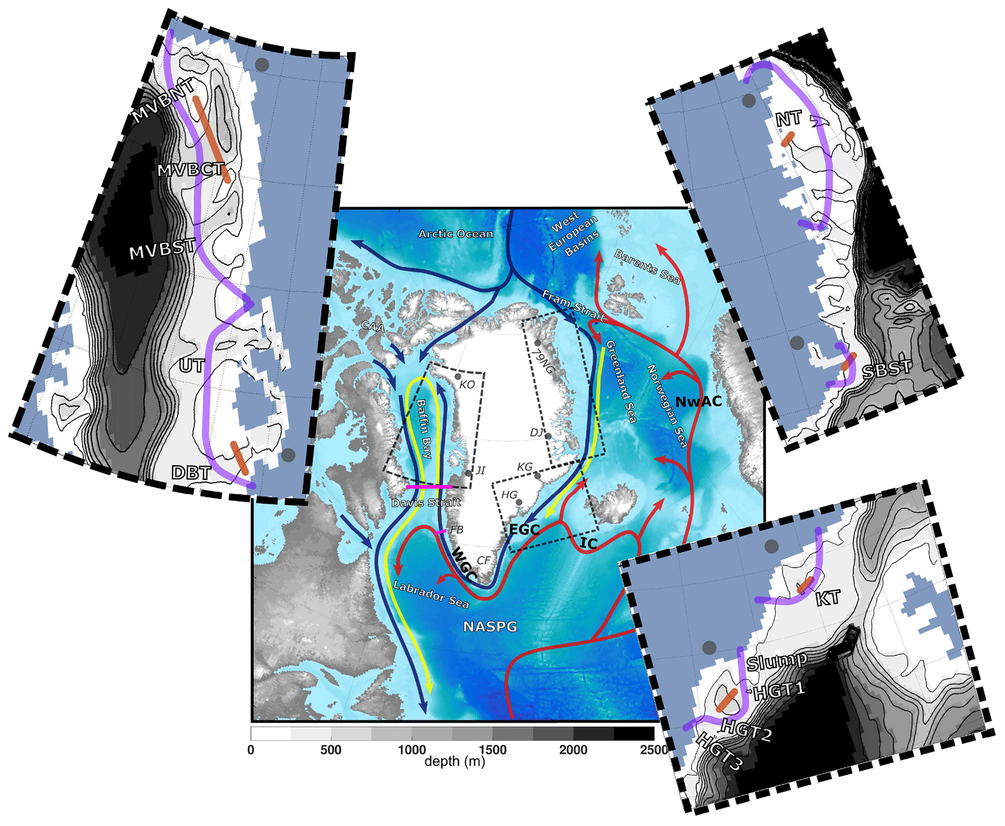
Figure 1Ocean circulation around Greenland with relatively warm Atlantic waters is shown in red, modified Atlantic waters are shown in yellow, and the Arctic and freshwater pathways are shown as blue lines. The large map's bathymetry and topography was generated using the ETOPO2 v2 dataset (National Geophysical Data Centre, 2006). This map shows areas that will be discussed throughout this study such as the North Atlantic Subpolar Gyre (NASPG), Labrador Sea, Davis Strait (section drawn in magenta), Baffin Bay, Canadian Arctic Archipelago (CAA), Arctic Ocean, West European Basins, Norwegian Sea, Greenland Sea, Fram Strait, Cape Farwell (CF), and Fylla Bank (FB) (section drawn in magenta). Ocean currents (adapted from Straneo et al., 2012; Hu and Myers, 2013) that will be discussed are shown here, Irminger Current (IC), Norwegian Atlantic Current (NwAC), East Greenland Current (EGC), and West Greenland Current (WGC). The light grey circles show the locations of six marine-terminating glaciers: Kong Oscar (KO) that terminates into Melville Bay (MVB), Jakobshavn Isbrae (JI) that terminates into Disko Bay (DB), Helheim Glacier (HG), Kangerlussuaq Glacier (KG), Daugaard-Jensen Glacier that terminates into Scoresby Sund (SBS), and Nioghalvfjerdsbrae (79NG). The insets show a closer view of specific regions around Greenland. Starting from the top left are the western, southeastern, and northeastern coasts. The insets show the model coastline, model bathymetry in metres (in grey shading and black contours), six sections of our analysis along the shelf in light purple, and sections of troughs (tan lines).
Along the shelf break of Greenland, transverse troughs extend from the coast supplying warm water through to the mouths of fjords. Then depending on the structure of the water mass at the mouth of the fjord and the height of the fjord's sills, warm waters can access marine-terminating glaciers and accelerate their mass loss (Straneo et al., 2012; Gladish et al., 2015b; Cai et al., 2017). If the warm waters from the NASPG can reach these transverse troughs, changes in the heat content of the NASPG may influence the state of marine-terminating glaciers on the GrIS.
This study investigates the following questions: how is the heat flux through the troughs affected by ocean model resolution? What is the mean and variability of the heat flux through the troughs around Greenland? What are the processes that drive the variability of the flux?
2.1 Model description
A general circulation coupled ocean–sea ice model is utilized in this study. The fundamental modelling framework used is the Nucleus for European Modelling of the Ocean (NEMO) version 3.4 (Madec, 2008). The ocean component is based on Océan Parallélisé (OPA) and is used for ocean dynamics and thermodynamics. For sea ice dynamics and thermodynamics, the Louvain la Neuve Ice Model (LIM2) is used (Fichefet and Morales Maqueda, 1997). The regional domain for the coupled ocean–sea ice model covers the Arctic Ocean and Northern Hemisphere Atlantic Ocean (ANHA), with two open boundaries: one at the Bering Strait and the other at the latitude of 20∘ S. All simulations start from January 2002 and are integrated to December 2016.
Initial and monthly open boundary conditions (temperature, salinity, horizontal velocities, and sea surface height) are derived from the 0.25∘ Global Ocean Reanalyses and Simulations (GLORYS2V3) product (Ferry et al., 2008). The surface atmospheric forcing fields (10 m surface wind, 2 m air temperature and humidity, downward shortwave and longwave radiation, and total precipitation) with a temporal resolution of 1 h and spatial resolution of 33 km are from the Canadian Meteorological Centres Global Deterministic Prediction System Reforecasts (CGRF), provided by Environment and Climate Change Canada (Smith et al., 2014). The first 2 years of the model output are regarded as the adjustment from the initial GLORYS2V3 fields, which have already had over 10 years to evolve. Figure 2 shows the monthly summation of total kinetic energy (KE) in all layers of Baffin Bay for the two experiments that will be discussed in detail in the next section, LowResControl and HighRes (Fig. 2a and b). The KE is low at the model start (January 2002) and increases abruptly after 2004 for the LowResControl experiment. For HighRes, the KE is fairly comparable for all years. HighRes also has more than an order of magnitude higher KE values compared to LowResControl. Figure 2 suggests that the spin-up of the large-scale Baffin Bay circulation from the initial conditions takes 1 to 2 years, although it would take much longer for the deep layer, and the interannual variation is not considered. Thus, only 5 d averaged model outputs from 2004 to 2016 are analyzed in this study.
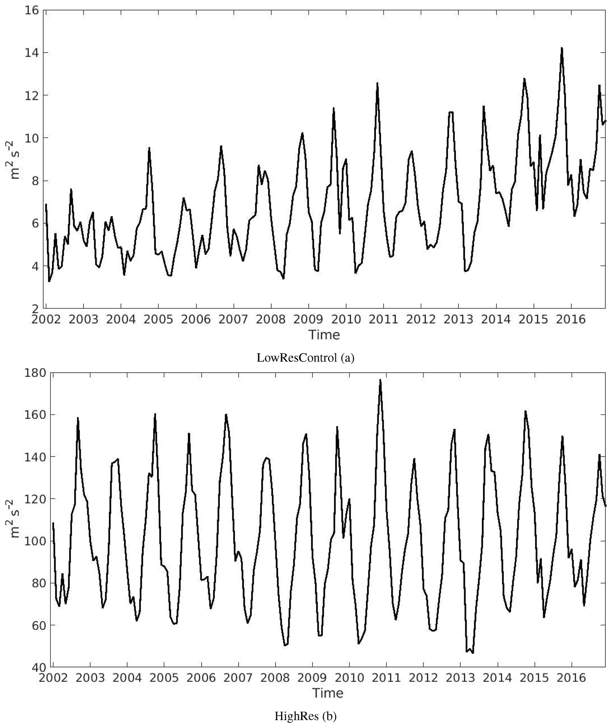
Figure 2Monthly summation of total kinetic energy in Baffin Bay for two experiments, LowResControl and HighRes.
2.2 Sensitivity experiment setup
2.2.1 Control experiment
The ANHA horizontal mesh grid is extracted from a global tripolar grid, ORCA (Barnier et al., 2007), at a 0.25∘ resolution (hereafter referred to as LowResControl for low resolution) with a resolution ranging from ∼11 to ∼15 km around Greenland. In the vertical, the LowResControl configuration uses the geopotential or z-level coordinate with a total of 50 levels. The layer thickness increases from 1.05 m at the surface level to 453.1 m in the last level (at a depth of 5727.92 m). Vertical high resolution is applied to the upper ocean, i.e., 22 levels for the top 100 m. Partial step (Bernard et al., 2006) is also enabled to better represent the sea floor. Bathymetry in LowResControl is taken from the existing global ORCA025 bathymetry (MEOM, 2013), which is based on a global relief model (ETOPO1) (Amante and Eakins, 2009) and a gridded bathymetric dataset (GEBCO1) (BODC, 2008) with modifications (Barnier et al., 2007).
This study will focus on the relatively large-scale processes outside of the fjords (as fjords are not resolved in this configuration) with an assumption that meltwater will reach the ocean surface once out of the fjord (Fig. 3). This assumption defines how Greenland discharge is added in the model, injected at the surface level then mixed into a 10 m thick layer. This approach is common in the present generation of ocean models at this horizontal scale, such as in Castro de la Guardia et al. (2015) and Dukhovskoy et al. (2016). Observations (Beaird et al., 2017, 2018) have shown that freshwater may not only be at the surface but be mixed and entrained with ambient waters and find a neutral buoyancy at depth. Therefore, this stratification assumption in this model may be misrepresenting plume dynamics that occur in fjords and may need to be rethought in future studies.

Figure 3The schematic shows how the model injects meltwater. The left side of the figure shows what the model cannot resolve. This includes a glacier, small-scale melting from the glacier, and the plume dynamics that occur along the face of the glacier. Instead, the model resolves larger-scale processes that occur along the coastline, and therefore injects the meltwater from the GrIS at the first ocean model layer at the surface, which then is mixed over a thickness of 10 m.
The LowResControl simulation uses two interannual monthly runoff sources. Greenland's freshwater flux (tundra and ice sheet runoff) is provided by Bamber et al. (2012) for 2002 to 2010, and the 2010 runoff is repeated for the last 6 years of this study. The ice sheet runoff includes surface melt and melt at the front edge of a glacier. Runoff in the rest of the model domain (not including Greenland) is provided by Dai et al. (2009). The model used in this study does not have an iceberg module, and thus only the ice sheet and tundra runoff are included from Greenland's freshwater flux (∼46 % of the total Bamber et al., 2012).
2.2.2 Changes in resolution
How is heat flux through the troughs affected by ocean model resolution? A 0.083∘ horizontal mesh grid is extracted from a global tripolar grid, ORCA (Barnier et al., 2007) (hereafter referred to as HighRes for high resolution), with a resolution ranging from ∼3.5 to ∼5 km around Greenland. The vertical resolution remains identical to the LowRes; however, the HighRes bathymetry is built based on partly different sources. The bathymetry is generated by using ETOPO1 (Amante and Eakins, 2009) for the polar region, and the Global Predicted Bathymetry (Smith and Sandwell, 1997) from satellite altimetry and ship depth soundings for the rest of the domain. Therefore, given the difference in the sources of bathymetry data, downscaling HighRes will not reduce to LowRes. The HighRes configuration provides model fields at a finer scale that is not always visible in LowRes. This provides the potential for a better simulation of warm ocean currents travelling towards the GrIS via better representation of deep troughs. In addition, the model resolution also plays a role in simulating ocean mixing and mesoscale features such as eddies, which bring warm water towards the GrIS shelf through the troughs. Note that, even at the 0.083∘ resolution referred to as HighRes in this study, the majority of the fjords are still not resolved. HighRes has the same runoff and Greenland's freshwater flux setup as LowResControl. Given the numerical cost of HighRes, LowResControl is utilized for the sensitivity experiments.
2.2.3 Enhanced Greenland discharge experiment
How can changing Greenland's freshwater flux impact the heat flux through the troughs around Greenland? As Castro de la Guardia et al. (2015) showed, enhanced Greenland melt can change nearby ocean circulation, e.g., spinning up the circulation in Baffin Bay. Here we compare a pair of experiments (LowResControl and LowResDoubleMelt) with the more realistic spatial distribution and temporally varying Greenland freshwater flux to quantify the impact on warm waters flowing towards the marine-terminating glaciers through troughs.
LowResControl under-represents the total of Greenland's freshwater flux. Therefore, LowResDoubleMelt takes into account the solid mass discharge. LowResDoubleMelt has the identical setup as LowResControl, except for Greenland's freshwater flux. It is important to note that the entire solid discharge in LowResDoubleMelt is transformed into the liquid component (i.e., treated the same as the runoff). In addition, the ocean does not affect GrIS melting as the melting is prescribed and non-interactive. This results in roughly twice as much freshwater flux (hereafter called meltwater) (100 % Greenland's freshwater flux, broken down by ∼46 % runoff and total iceberg discharge ∼54 %) in LowResDoubleMelt compared to LowResControl (roughly 46 % of Greenland's freshwater flux, only including runoff). Therefore, the total meltwater added to LowResDoubleMelt had been roughly doubled and actually has a more realistic amount of meltwater than LowResControl. For this study, a comparison of the GrIS meltwater is made to demonstrate the ocean model's sensitivity to increased GrIS melt. How will ocean temperatures in troughs that terminate into Baffin Bay be impacted by an increase in GrIS melt?
2.2.4 High-frequency atmospheric event experiment
Previous studies (Holdsworth and Myers, 2015; Garcia-Quintana et al., 2019), have shown that high-frequency atmospheric phenomena, such as storms, barrier winds, fronts, and topographic jets, play an important role in ocean processes (e.g., deep convection in the Labrador Sea) in the study area. Jackson et al. (2014) reported that synoptic events can impact water properties and heat content within two large outlet fjords. Therefore, they could impact shelf exchange and the renewal of warm waters to the GrIS. This study aims to go beyond the two fjords of Jackson et al. (2014) by considering the entire coast of Greenland.
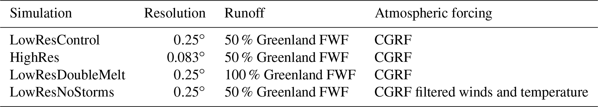
We use the Kolmogorov–Zurbenko (KZ) filter method (Zurbenko et al., 1996), as Eskridge et al. (1997) has shown that this filter has the same level of accuracy as the wavelet transformation method but is much easier to use. The KZ filter is based on an iterative moving average that removes high-frequency variations. We apply the moving average over a length of 10 d with one iteration, as Garcia-Quintana et al. (2019) has done previously. Therefore, the removal of atmospheric variability that persisted for 10 d or less from the atmospheric forcing was done to drive a sensitivity simulation, called LowResNoStorms. LowResNoStorms has an identical setup to LowResControl, except for the KZ filter applied in the wind and air temperature fields. For more information regarding the methodology of the KZ filtering, please see Zurbenko et al. (1996) and Eskridge et al. (1997). A complete list of simulations used in this study is given in Table 1.
Table 1ANHA-NEMO simulations used in this study. All experiments include interannual river discharge from Dai et al. (2009), except for the Greenland region, which is obtained by the Greenland Freshwater Flux (FWF) provided by Bamber et al. (2012). All simulations use the same atmospheric forcing, CGRF (Smith et al., 2014), but with the winds and air temperature filtered in LowResNoStorms.
2.3 Mean flow and its fluctuation
To evaluate the ocean's heat that reaches onto the shelf and into the troughs, heat fluxes are calculated at six sections along the coast of Greenland (across one trough per section, as shown in purple and tan, respectively, in Fig. 1). Section names and their associated trough names are seen in Fig. 1. To calculate the fluctuation of the heat flux, the 5 d average model outputs of both temperature (T) and velocity (U) normal to the section are treated as the full current. A moving average (Eq. 2) was applied by averaging five model outputs (25 d) centred on a particular output (n) by taking outputs from two previous outputs ((n−2) and (n−1)), the centred output (n), and two future ((n+1) and (n+2)). A test has been previously done (not shown) for a different averaging timescale of 85 d (roughly 3 months) and 185 d (roughly 6 months) and found that the different timescale averaging did not significantly change the results. Therefore, the mean of the temperature and velocity (, ) were taken over 25 d. The mean values were then subtracted from the full current to get the fluctuation component of the heat flux in Eq. (3). Given Eq. (3), ρ0 is the reference density, Cp is the specific heat capacity of seawater, L is the length along the section direction x, H(z,x) is the water depth along the section, and is the velocity normal to the section.
To determine heat content and heat transport, a reference temperature has to be used. We considered using 0 ∘C, given glacial ice is fresh and 0 ∘C is the melting point for freshwater ice. However, there is a strong dependency on the freezing point on salinity and pressure. The boundary layer salinity is, in general, not zero (Holland and Jenkins, 1999). Further, the pressure dependence of the freezing point is significant; even for freshwater at ∼700 m, the freezing point drops by half a degree. Thus, following a suggestion from a reviewer and assuming moderate boundary layer salinities, we choose a reference temperature of ∘C (271.65 K). Where there is little below-zero water, the choice of reference temperature will not make much difference. Where there are significant amounts of below-zero water, such as off northeastern Greenland, our estimates then become a potential upper bound on the amount of heat available for glacial melting, assuming salinity and pressure have depressed the glacial freezing point from 0 ∘C. Therefore, T is the temperature in Celsius with Tref taken into account, and T0 is the original model temperature field (Eq. 1).
To see the importance of the fluctuation component of the flow around Greenland, the transient kinetic energy (TKE) was calculated using Eq. (4); u and v are the 5 d averaged model outputs of the zonal and the meridional velocity and and denote the monthly mean averages.
2.4 Model evaluation
To continue with this study, a comparison was done to make sure that the model behaves similar to observations for West Greenland waters. The water mass structure at Fylla Bank is compared to observations from Ribergaard (2014). This section is chosen, as the WGC branches shortly after passing Fylla Bank, with a portion moving westward and joining the Labrador Current, while the other portion continues north through Davis Strait. The Fylla Bank section is shown with a magenta line in Fig. 1 (red in Fig. 1 in Ribergaard, 2014). The observed temperature and salinity for 14 June 2013 (Fig. 31 in Ribergaard, 2014) are compared to the modelled averages for June 2013 (Fig. 4). LowResControl (Fig. 4a) had a similar water mass structure to the observations. In both observations and LowResControl, there was cooler water at the surface with a thickness of 50 m offshore and about 100 m thick, just off the west side of the bank (kilometre marker 45 in Fig. 4a), with warmer water (greater than 3 ∘C) below 100 m depth. The cold water layer in LowResControl was slightly saltier with the depth of the modelled 34.2 isohaline, similar to that of the observed 34 isohaline (Fig. 31 in Ribergaard, 2014). For HighRes, the cold surface layer was thicker (Fig. 4b) than in observations, where the 2 ∘C layer (contour in magenta) extended to about 100 m depth off the west side of Fylla Bank at kilometre marker 45. Similar to observations the 4 ∘C and warmer water mass starts below 200 m and slopes upwards towards the west. At a depth of ∼400 m, HighRes is warmer than observations by ∼1 ∘C. Overall, the modelled water mass structure compared well with the observations but had minor offsets in temperature and salinity. The model had a shallow fresh and colder surface layer in the west portion of the section that deepened towards Fylla Bank. Finally, the HighRes configuration had a much sharper and better-represented thermocline in comparison to the LowResControl configuration.
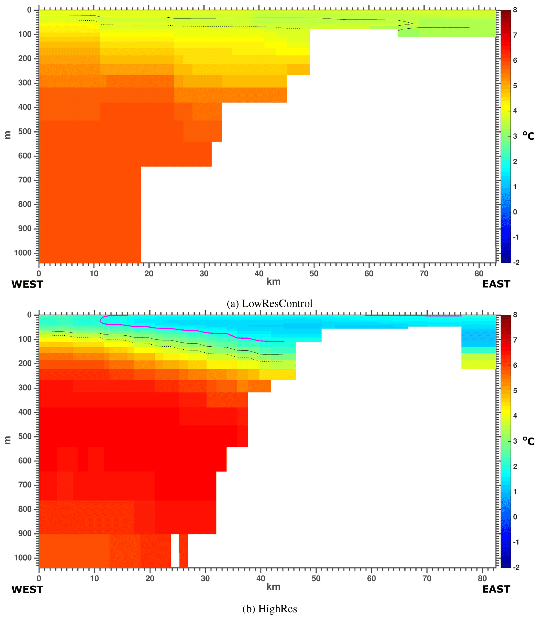
Figure 4Average Fylla Bank temperature for June 2013 for (a) LowResControl and (b) HighRes. The magenta line shows the 2 ∘C isotherm, the black line is the 34.0 salinity isohaline, and the dashed black line is the 34.2 salinity isohaline.
Moving northward to the Davis Strait, the primary gateway for meltwater and heat exchange between Baffin Bay and the North Atlantic Ocean, we look at the model and the observations. A comparison was done with LowResControl and HighRes to the Curry et al. (2014) moored array data (see Fig. 2 in Curry et al., 2014). The monthly modelled temperature averaged over 2004–2010 at Davis Strait (Figs. 5 and Fig. 6) was compared to the mooring observations (Curry et al., 2014, their Fig. 3c). From July to September LowResControl (Fig. 5) captured the same structure of the West Greenland Slope Water (WGSW) and West Greenland Irminger Water (WGIW), as in the Curry et al. (2014) study. See Table 2 for water mass characteristics in Davis Strait. From March to June LowResControl showed WGIW and WGSW were cooler (∼3 ∘C) by about a degree than in the observations (∼4 ∘C). LowResControl also had a tongue of relatively warm water from the WGIW protruding into the interior of Davis Strait at ∼200 km and ∼200 m depth. For HighRes (Fig. 6), the structure was similar to that of LowResControl, with the protruding tongue at ∼200 km and ∼200 m depth. HighRes also had a similar structure to the observations for the WGSW from July to October. Note that compared to observation, the WGSW and WGIW seem to be about 1 ∘C warmer.
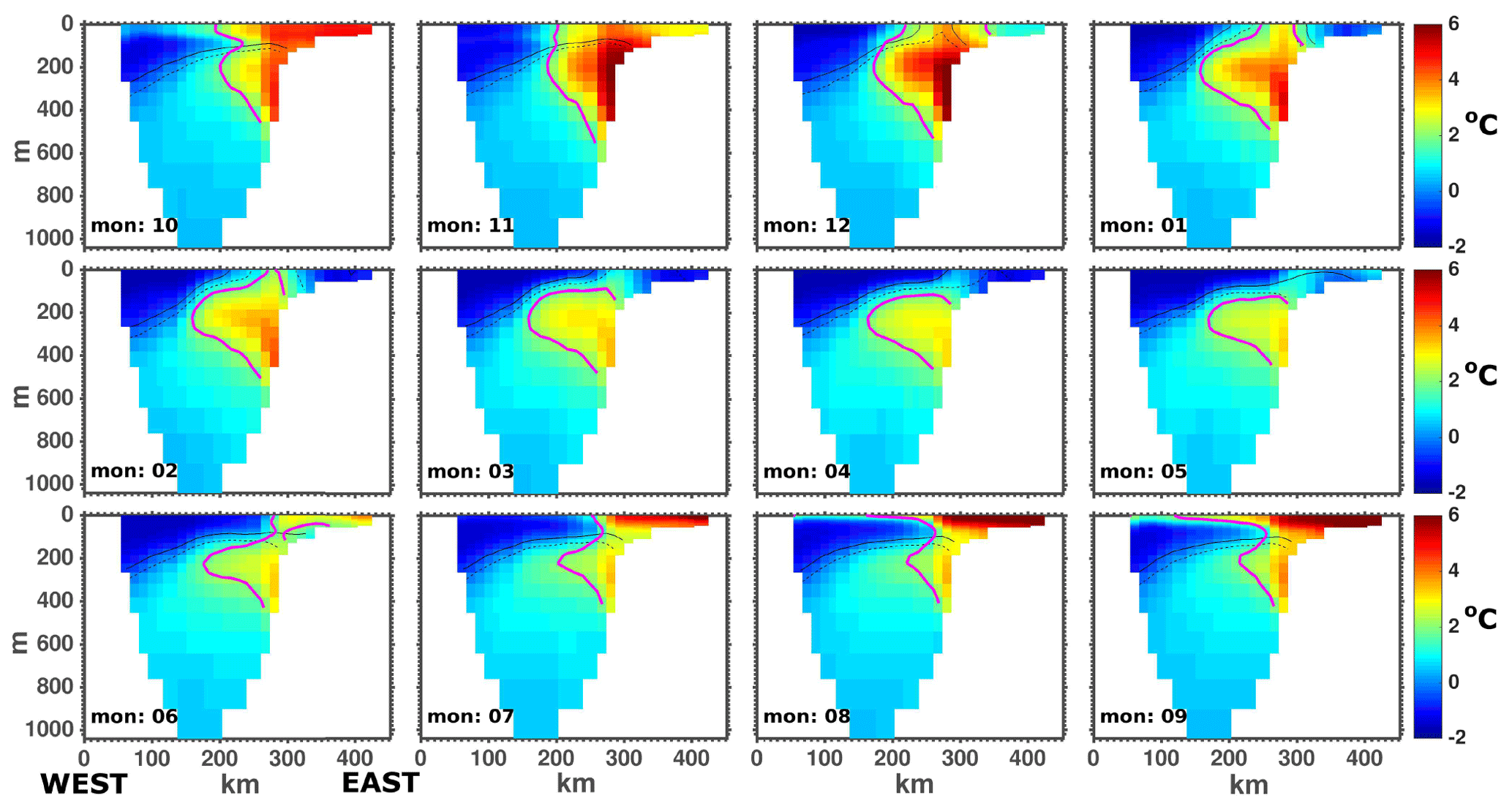
Figure 5The monthly average temperature through the period of 2004 to 2010 at Davis Strait from LowResControl. The magenta line represents the 2 ∘C isotherm, the black line is the 34.0 salinity isohaline, and the dashed black line is the 34.2 salinity isohaline.
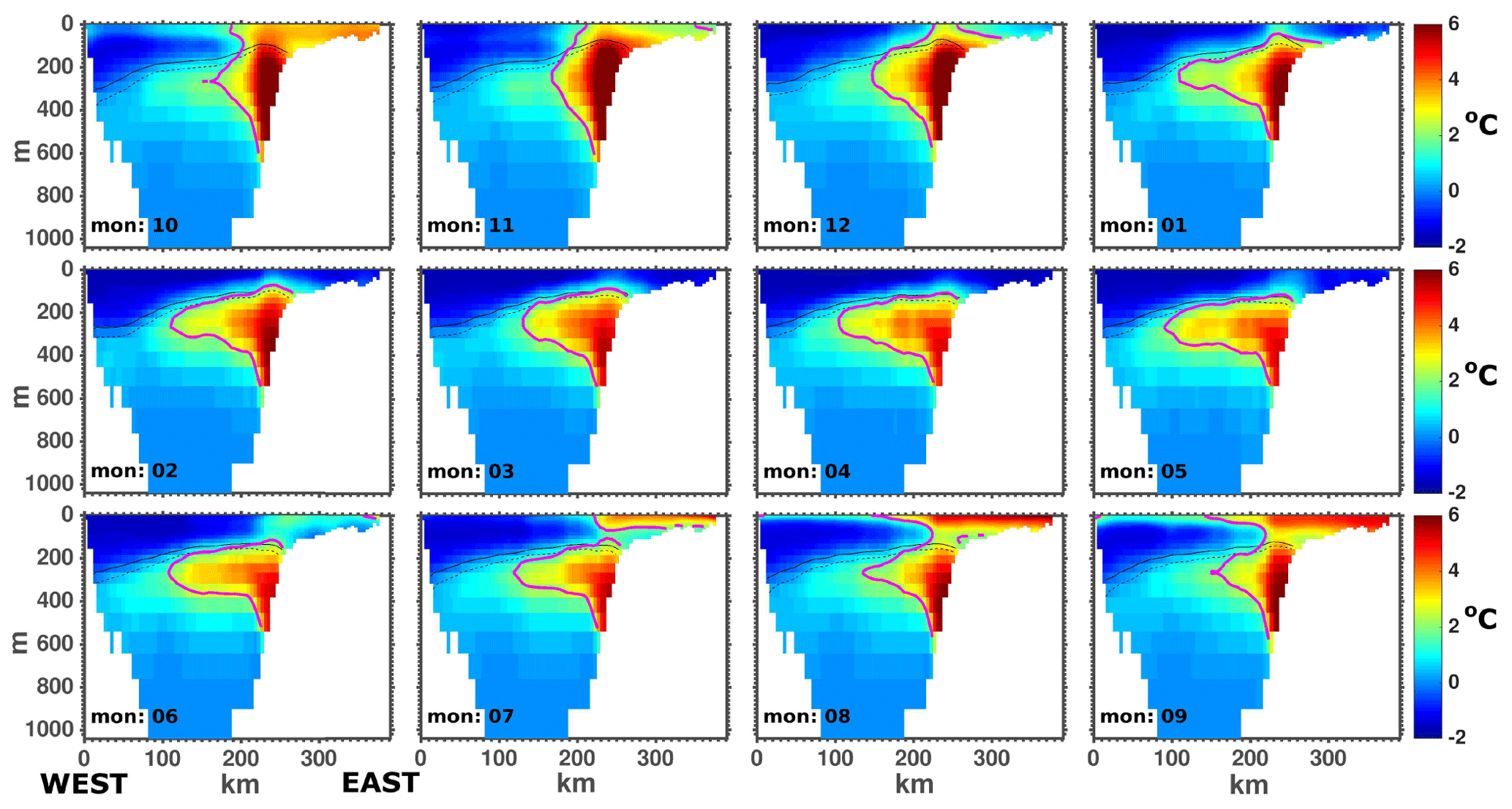
Figure 6The monthly average temperature through the period of 2004 to 2010 at Davis Strait from HighRes. The magenta line represents the 2 ∘C isotherm, the black line is the 34.0 salinity isohaline, and the dashed black line is the 34.2 salinity isohaline.
Table 2Overview of Davis Strait's water masses. Potential temperature (θ) and salinity (S) characteristics are as defined by Curry et al. (2011).

Curry et al. (2011) plotted a temperature and salinity (TS) diagram (their Fig. 3) showing the main water masses (Table 2) at Davis Strait, based on September 2004 and 2005 data along the mooring line. This plot was repeated using all September and October observational data collected within ∼30 km of the Davis Strait sill as part of the Davis Strait programme from 2004 to 2010 (Fig. 7). Although the result is denser, the same general structure as in Curry et al. (2011) can be seen. HighRes and LowResControl are plotted similarly (September and October fields, for the same region as the observations, from 2004 to 2010). HighRes shows a similar structure for the WGIW and WGSW, while LowResControl's WGSW is warmer and its WGIW does not show the same tail-off to lower salinities with its transitional water between 2 and 0 ∘C. Both runs show polar water with a salinity between 32.5 and 33.5, which is about a degree warmer than the observations and then warming to 1 to 2 ∘C as the salinity drops to 31.
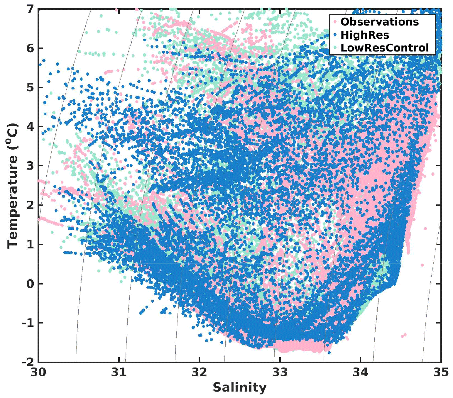
Figure 7Temperature and salinity plot for the region around the Davis Strait sill (∼30 km). Observations contain data collected by the Davis Strait program's fall mooring cruises. Observations are taken in the fall months, late August to October, for the years 2004 to 2010. Model fields are plotted the same for HighRes and LowRes Control (mid-September and mid-October fields, within ∼30 km of the Davis Strait sill, from 2004 to 2010). Model fields are subsampled to a 0.5∘ grid to reduce the number of points plotted. Points with a salinity of less than 30 or more than 35 or that are warmer than 7 ∘C are excluded. Thin curved black lines are density in given in values of kilograms per cubic metre.
The LowResControl and HighRes volume transport from September 2004 to September 2013 (Fig. 8) can satisfactorily represent the observations from the mooring array at Davis Strait (e.g., Curry et al., 2011, 2014). Positive values indicate southward volume fluxes through Davis Strait, and negative values indicate northward transport. All model and observation outputs are plotted as the same 5 d average. The simulations underestimated the high-frequency peaks of transport from the observations (values approaching 6 Sv in some cases). The mean volume flux based on the Davis Strait moorings (Curry et al., 2011, 2014), calculated over the period of 21 September 2004 to 30 September 2013 is 1.6 Sv. Over the same period, the model transports are 1.2 Sv for LowResControl, with a correlation of 0.54, significant at the 99 % level, and 1.2 Sv for HighRes, with a correlation of 0.49. Yet many features, such as the reduction in transport at the end of 2010, are well simulated.
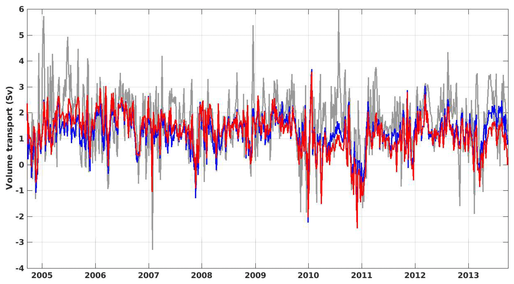
Figure 8Volume flux through Davis Strait with HighRes (in red), LowResControl (in blue), and Davis Strait observations replotted from the mooring record discussed in Curry et al. (2014) (in grey). Positive values indicate southward volume fluxes through Davis Strait, and negative values indicate that the waters move northward. All fields, models, and observations are plotted as 5 d averages.
2.5 Study area
This study focuses on six sections around Greenland (Fig. 1) with marine-terminating glaciers and deep bathymetric features. In Fig. 9 the six sections are shown (seen in light purple on the map inset in Fig. 1). HighRes model bathymetry is in grey and each section runs north to south on the x axis starting on the left-hand side of the figure indicated by the 0 km marker. The rest of this section will compare the six sections and discuss how observed bathymetry from other studies compares to the HighRes model bathymetry (Fig. 9).
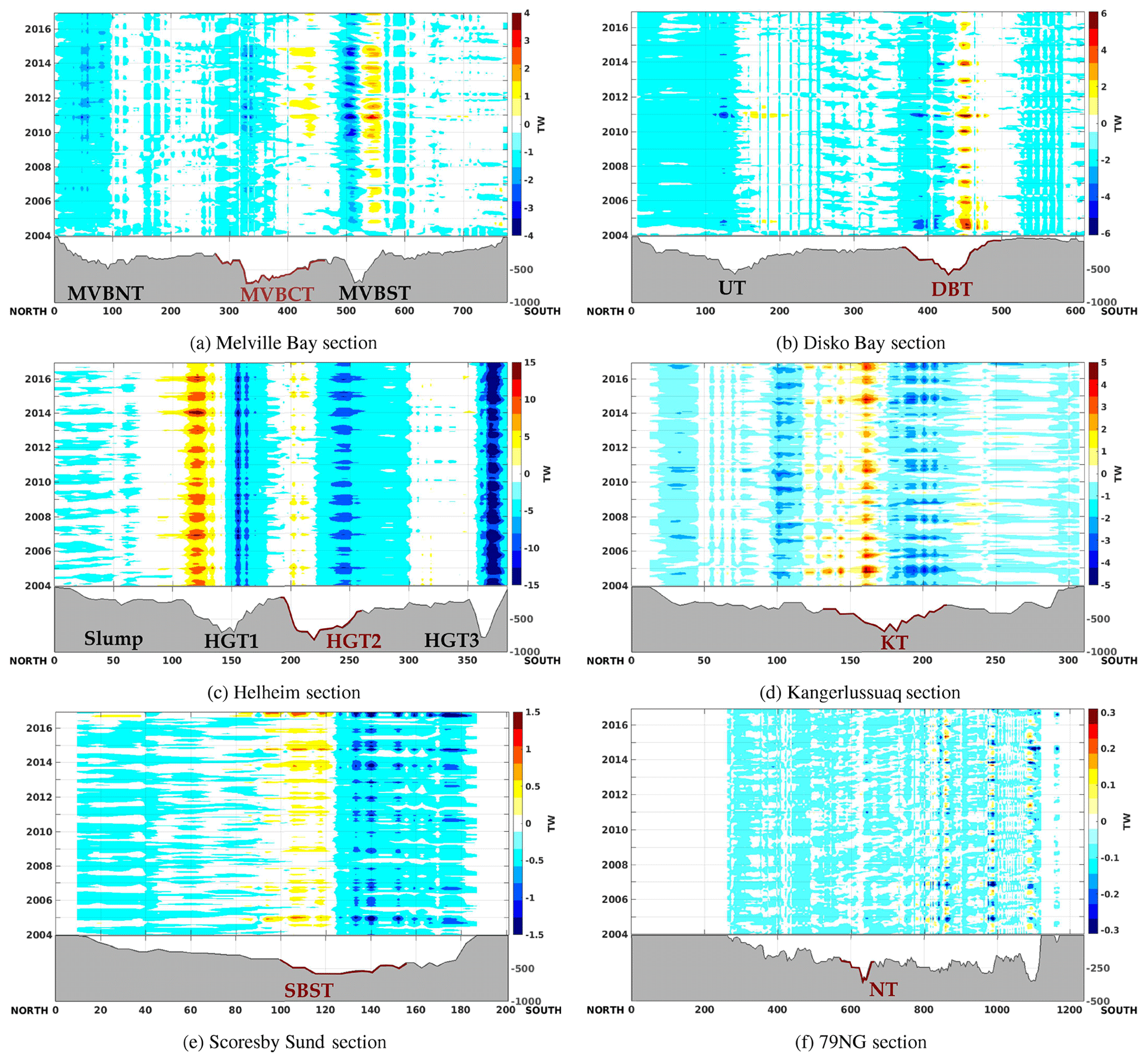
Figure 9This figure shows the entire ocean heat exchange (total flux) with respect to topography (in grey) within the time series from 2004 to the end of 2016 with the HighRes model output. These Hovmöller plots show the monthly average heat flux coming on or off the shelf in TW, through a section (sections drawn in light purple on the map inset Fig. 1). Model bathymetry is in grey and the section runs north to south on the x axis, starting at the left-hand side of the figure indicated by the 0 km marker. Along the y axis is the depth for the bathymetry and then time for the 2004 to 2016 period. Colours indicate the direction and magnitude of the onshore or offshore heat flux. Positive numbers indicate the direction of onshore heat flux, and negative numbers indicate the direction of the heat flux offshore. Colour bar limits change per location. Each section shows a highlighted trough in dark red, which is selected for Figs. 10 and . Figure 1 indicates the exact location of the trough as tan lines.
In northwestern Greenland, Kong Oscar Glacier is the fastest marine-terminating glacier, terminating into Melville Bay (Rignot and Kanagaratnam, 2006; Rignot and Mouginot, 2012). A total of 20 % of the GrIS drainage volume is directed along glaciers that feed into Melville Bay, amounting to a discharge of ∼80 km3 yr−1 (Rignot and Kanagaratnam, 2006). Located in northeastern Baffin Bay (Fig. 1), Melville Bay holds the widest and deepest Greenland cross-shelf troughs. This system consists of three troughs: the northern, central, and southern Melville Bay troughs (MVBTs: MVBNT, MVBCT, and MVBST). The MVBTs are 170 to 320 km long, 45 to 120 km wide, and reach depths between 740 and 1100 m with shallow banks (around 100 m below sea level) called inter-trough banks (Slabon et al., 2016; Morlighem et al., 2017). The HighRes bathymetry (seen in Fig. 9a) is relatively shallow compared to the observations discussed. MVBNT is located at the indicated markers for 10 to 120 km, MVBCT is located at 320 to 450 km, and MVBST is located at 480 to 580 km. The depths in the HighRes model are about 400 m for MVBNT, reaching almost 700 m depth for MVBCT and MVBST.
Further south, on the western coast of Greenland, Jakobshavn Isbrae (JI) terminates into Disko Bay. The rapid retreat and disintegration of JI's floating ice tongue have been attributed to an increase in heat content, deep bathymetry, and NASPG warming (Holland et al., 2008; Myers and Ribergaard, 2013; Gladish et al., 2015a; An et al., 2017). Recent slowing down of JI's acceleration has been attributed to the glacier reaching a higher bed, high amounts of freshwater from the Canadian Arctic, a weak WGC, or a cold Baffin Bay current flooding the West Greenland Shelf and cooling in the Labrador and Irminger Seas (Joughin et al., 2012; Gladish et al., 2015a; An et al., 2017; Khazendar et al., 2019). In HighRes, the section drawn for Disko Bay (Fig. 9b) shows two deep bathymetric features: the first trough, located at 100 to 200 km, and the second trough at 380 to 500 km, now called UT (Uummannaq trough) and DBT (Disko Bay trough), respectively. UT connects to Uummannaq Fjord and DBT connects into Disko Bay. Both UT and DBT reach depths of around 500 m, similar to observations found in Hogan et al. (2016). In a more recent dataset provided by BedMachineV3, UT similarly reaches approximately 500 m, but DBT is much deeper, reaching depths of 900 m (Morlighem et al., 2017).
In the southeastern region, there are two major glaciers of interest: Helheim Glacier (HG) and Kangerlussuaq Glacier (KG). HG terminates at a depth of 700 m in Sermilik Fjord, which is approximately 900 m deep at the U shape mouth with the adjacent continental shelf, reaching depths of 350 m (Straneo et al., 2010; Morlighem et al., 2017). Temperature variability in Sermilik Fjord cannot be explained by local heating or surface fluxes. The temperature variability in the fjord is instead a result of the advection of warmer waters into the fjord, as warm waters are present on the shelf year-round, peaking from July to September (Straneo et al., 2010). In HighRes, the section for HG (Fig. 9c) shows four unique features. The first one from the 25 km to about 100 km markers shows a slumping of bathymetry reaching about 250 m in depth. Moving further south, there are three deep troughs. The first trough is located at 120 to 180 km, reaching depths surpassing 500 m, and the second and third troughs are located at 190 to 260 and 350 to 375 km, respectively, reaching depths closer to 700 m. These features will be referred to as Slump, HGT1, HGT2, and HGT3.
In the BedMachineV3 dataset, Kangerlussuaq trough (KT) reaches depths closer to 800 m (Morlighem et al., 2017). Atlantic water occupies the deep waters of the KT and Kangerlussuaq Fjord (KF) (Azetsu-Scott and Tan, 1997). KF, similar to Sermilik Fjord, has a deep open mouth, which could influence the Atlantic water transport that is observed there (Azetsu-Scott and Tan, 1997; Christoffersen et al., 2011; Inall et al., 2014). In HighRes, the section drawn for KT (Fig. 9d) is drawn over an area with the maximum depth in the middle of the section, deeper than 600 m, at the 175 km marker. The KT extends from 125 to about 200 km.
In the northeast, Daugaard-Jensen Glacier terminates into Scoresby Sund and Nioghalvfjerdsbrae (79NG) terminates into the sound of Jøkelbugten. The BedMachineV3 shows depths of around 600 m (Morlighem et al., 2017). The HighRes section drawn for Scoresby Sund (Fig. 9e) is outside of the opening of the coastline, from north to south, connecting fjord waters to the open ocean. The bathymetry here is smoother with fewer carved features. Instead, it shows a skewed U shape in this section. The maximum depth is reached at the 120 km marker with a depth slightly greater than 500 m.
Nioghalvfjerdsbrae has a floating ice tongue that abuts Hovgaard Ø, which divides the tongue into two sections (Wilson and Straneo, 2015). The most rapid melting occurs at the grounded (pinned) front, south of Hovgaard Ø, where the ice tongue is thickest and is exposed to deeper and warmer waters (Mayer et al., 2000; Seroussi et al., 2011; Wilson and Straneo, 2015). Schaffer et al. (2017) showed that Atlantic Intermediate Water flows via bathymetric channels to the south of Hovgaard Ø at a pinned ice front, where there is a shorter pathway between the shelf and cavity, exposing the cavity to more shelf driven processes such as intermediary flows. The warm water is supplied from the warm water that resides in Norske trough (NT) east of Hovgaard Ø (Fig. 1) (Wilson and Straneo, 2015). Some of the relatively fresh glacially modified water is exported to the continental shelf via Dijmphna Sund, north of the glacier (Wilson and Straneo, 2015). In BedMachineV3, NT reaches depths close to 600 m (Morlighem et al., 2017). The HighRes section drawn for 79NG (Fig. 9f) is drawn from north to south. The HighRes bathymetry shows the deepest region exceeding depths of 300 m, though the majority of this section lies around 200 m.
3.1 Onshore heat flux through coastal troughs
What is the significance of the deep troughs along Greenland's shelf to the supply of warm water to the fjords with marine-terminating glaciers? A look at the onshore heat flux through these troughs will be shown using HighRes, as the benefits of a higher horizontal resolution have been shown. However, given the numerical costs of the HighRes model, LowResControl is utilized for the sensitivity experiments that will be discussed later in this paper.
3.1.1 Western coast: mean state
A section was drawn for Melville Bay (Fig. 9a), located on the northwestern coast of Greenland, which shows three deep bathymetric troughs: the MVBNT, MVBCT, and MVBST (all troughs described in Sect. 2.5). At the northern edge of all three troughs (the 50, 330, and 500 km markers for MVBNT, MVBCT, and MVBST, respectively) there is an offshore heat flux. At the southern edge of all three troughs (the 110, 450, and 560 km markers for MVBNT, MVBCT, and MVBST, respectively) there is an onshore heat flux. This identified that the northward warm waters travelling along the western coast of Greenland are influenced by bathymetry and are steered eastward along the trough towards the coast.
MVBNT, the shallowest of the troughs, had the weakest onshore heat flux, barely exceeding 0 TW. MVBCT and MVBST transport increased between 2009 and 2010 and persisted in an anomalously high state for 5 years. For MVBNT there was an increase in onshore heat transfer for a brief period in 2010 (0.5 TW). At MVBCT an increase in heat flux started at the end of 2009 and reached a relatively stable value of 1 TW through to the end of 2015. For MVBST there was a more persistent interannual heat flux throughout the entire time period, increasing from 1 to 3 TW starting at the end of 2009. An increase in heat flux through troughs in northern regions of the Greenland Shelf starting in 2009 for MVBCT and 2010 for MVBNT and MVBST was thus identified. A change of 1 TW is significant, as that increase in heat can potentially melt 3000 t of ice per second. Thus, an increase in ocean heat presence in these troughs may have driven more melt from the glaciers that terminate in Melville Bay.
A section drawn for Disko Bay (Fig. 9b), located on the western coast of Greenland, shows two deep troughs: UT and DBT. Both troughs showed an onshore heat flux at the southern edge (around the 180 and 480 km markers for UT and DBT, respectively) and an offshore heat flux at the northern edge (100 to 120 and 400 to 420 km markers for UT and DBT, respectively). This section, as well as the Melville Bay section, showed that the ocean currents are influenced by the bathymetry and are steered eastward into the trough towards the coast.
There was an onshore heat flux into DBT in the early 2000s that was consistently strong from 2004 to the end of 2007. Another increase in the heat flux (values showing 6 TW) were seen later on, reaching a maximum in 2010 and then decreasing back towards 4 TW afterward. The increased heat flux from 2004 to 2006 coincided with the disintegration of the JI floating tongue and was within the period of observed oceanic heat increase in Disko Bay (from 1997 to 2007) (Holland et al., 2008). For UT there are pulses of onshore heat flux of about 1 TW throughout the period. Through 2010 to 2012 there are variable pulses (1 TW), with a maximum in the winter of 2010–2011 with a value of 2 TW.
3.1.2 Western coast: seasonal and interannual variation
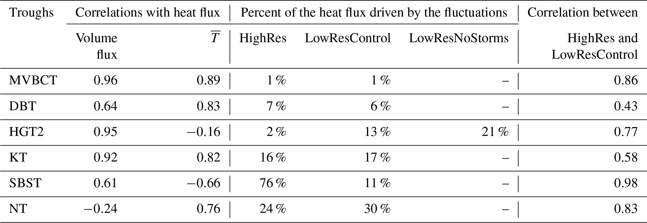
The seasonality of the onshore heat flux is shown in MVBCT (Fig. 10a). Late fall and early winter showed the maximum onshore heat flux with a peak in November. Through late winter to spring the onshore heat flux is weakest with the minimum being in April. The years 2004–2007, as indicated in a variety of blues in Fig. 10, overall had less onshore heat flux. As time progressed, the onshore heat flux increased. The years 2010, 2011, and 2014 (as indicated in colours of pale green and orange) showed the highest values of onshore heat flux, reaching maxima of about 15 to 19 TW. This increase in heat flux indicates that more heat has been brought into MVBCT in more recent years. The lack of a summer peak at MVBCT, suggests seasonality is dominated by the subsurface warm layer. MVBCT heat flux seasonality seems to be dependent on both the seasonality of the volume flux and temperature (Fig. 10b and c), respectively, with a correlation of 0.96 and 0.89 (shown in Table 3).
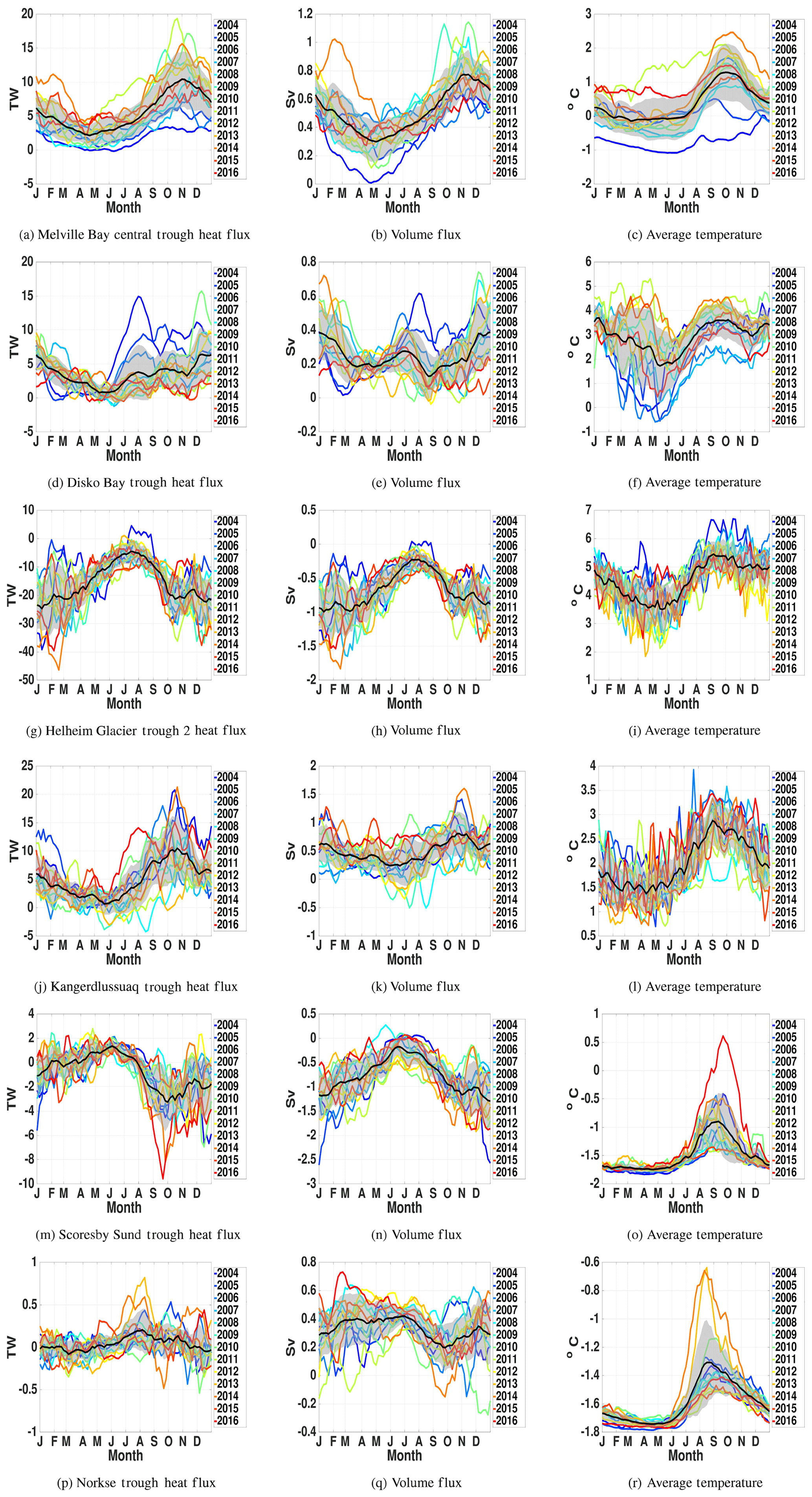
Figure 10Seasonality of the heat flux (unit: TW; 1 TW =1012 W), volume flux (unit: Sv; 1 Sv=106 m3 s−1) and section-averaged temperature (unit: ∘C) in MVBCT, DBT, KT, SBST, and NT (locations shown in Fig. 1) for each year from 2004 to 2016 (colour codes are shown in the legend). Note that the black line shows the mean of the 25 d moving-window averages (Eq. 3) over 2004 to 2016, with the standard deviation shown by the grey shading.
Table 3This table shows a comparison for the entire time series (2004 to 2016) of the different troughs along the shelf of the GrIS: Melville Bay central trough (MVBCT), Disko Bay trough (DBT), Helheim Glacier trough 2 (HGT2), Kangerlussuaq trough (KT), Scoresby Sund trough (SBST), and Norske trough (NT). These troughs can be identified in Fig. 1. The second and third columns show the correlation between the heat flux with the volume flux and the average temperature () across the section (shown as a black line in Fig. 10). The fourth, fifth, and sixth columns show the average percent of the heat flux moderated by fluctuations from three configurations, HighRes, LowResControl, and LowResNoStorms, respectively. Column seven shows the correlation between the total heat flux (mean and fluctuation) from two configurations: HighRes and LowResControl.
Further south in DBT (Fig. 10d), the fall and winter seasons have stronger onshore heat flux. However, earlier years (2004 to 2005) show above-average onshore heat flux in the summer. Maximum onshore heat flux was identified in July and August of 2004 and 2005 (reaching values around 10 to 15 TW). However, in other years, June and July have lower values of heat flux (hovering close to 4 TW). This warming event from 2004 to 2006 is also seen in DBT in Fig. 9b. In 2010 there was a spike in onshore heat flux in December, reaching over 15 TW, which then decreased in January (Fig. 10d). Enhanced heat flux in 2011 was seen in UT and MVBST (Fig. 9a and b), indicating that the warming event was a large-scale rather than a localized process. The timing of the onshore heat flux peak also undergoes large interannual variation (Fig. 10d), which is likely driven by the volume flux of the inflow (Fig. 10e)
Observations at Davis Strait show a temperature maximum starting around August–September that continues through to November–December (Curry et al., 2011; Grist et al., 2014). However, heat flux peaks in DBT occurred as early as June–July between 2004 and 2006 (Fig. 10d), suggesting a larger influence from the warm surface waters in these months. As the years progressed in the model, the timing of the maximum heat flux was delayed until later in the year to between September to January, albeit with significant inter-annual variability. This timing coincided with the peak of warmest Irminger Water observed in Davis Strait. The timing was due to the advection time needed by the Irminger Sea water. Given they are farther north, the warm water reached Melville Bay later in the year than Disko Bay. This lag in the seasonal cycle of warm water is consistent with the Lagrangian trajectory-based study by Grist et al. (2014).
The results (Fig. 10d) showed that an early arrival of warm waters (June in 2004) occurred at the time when JI started to melted rapidly (Holland et al., 2008). This may, therefore, have been due to not only an increase in ocean heat flux but perhaps also an arrival of warm waters earlier in the melt season impacting JI for a longer duration. DBT heat flux seasonality is more dependent on the seasonality of the temperature of the water mass and less dependent on the seasonality of the volume flux (Fig. 10f and e), with a correlation of 0.64 with the volume flux and 0.83 for the temperature (shown in Table 3).
3.1.3 Southeastern coast: mean state
The section drawn for Helheim (Fig. 9c), located off the southeastern coast of Greenland, shows four unique features, Slump, HGT1, HGT2, and HGT3. At the northern edge of the troughs in this section, HGT1 through to HGT3, (the 100, 200, and 350 km markers) there is an onshore heat flux and an offshore heat flux at the southern edge (the 175, 225, and 355 km markers). This identifies that there must be southward-flowing warm water travelling along the southeastern coast of Greenland, potentially drawn in from the Irminger Current, and that the warm waters are again being bathymetrically steered westward along the trough towards the coast. Slump showed weak offshore heat flux, oscillating from 0 TW to TW, potentially associated with transient mixing and eddies.
The section that is drawn for KT (Fig. 9d) highlights the extent of this trough. In the northern portion of the section, from about 25 to 100 km, there is evidence of mixing of signals of onshore and offshore heat fluxes. At the 160 km mark, throughout the years, there is a onshore heat flux of greater than 2 TW and there is an offshore heat flux on the southern edge of the trough of a similar magnitude. In the southern portion of the section (from 225 to 325 km) there is variability in the offshore heat flux in space and time.
3.1.4 Southeastern coast: seasonal and interannual variation
For HGT2 (Fig. 10g) the sign of the heat flux is mostly negative (offshore), with the highest magnitude occurring between the period of August through to May. Offshore heat flux occurred year-round (except for short bursts in 2005) making this location unique compared to all other regions examined. Observations from a fjord in southeastern Greenland (Sermilik Fjord) showed that water properties and heat content vary significantly on synoptic timescales throughout non-summer months (Jackson et al., 2014). Looking at HGT2 (Fig. 10g), from October to March there was large variability in the magnitude of the heat flux and also a decrease in average temperature (Fig. 10i).
The seasonality of HGT2 heat flux is dominated by that of the volume flux (correlation of 0.95) (Fig. 10h), while the seasonality of the averaged temperature is out of phase (correlation of −0.16) (Fig. 10i). At KT (Fig. 10j), the seasonality of heat flux seems to be dependent on both the seasonality of the volume flux and temperature (Fig. 10k and l), with a correlation of 0.92 and 0.82, respectively (Table 3). At KT, the peak of onshore heat flux occurred after August for most years with significant interannual variation. The stronger warming events were found in 2004, 2005, 2014, and 2016.
3.1.5 Northeastern coast: mean state
The section drawn for Scoresby Sund (Fig. 9e) shows Scoresby Sund trough (SBST). On the trough's northern edge near the maximum depth, at the 110 km marker, there is a consistent signal for the onshore heat flux of more than 0.5 TW. The strongest offshore flux, at the 120–180 km marker, reaches −1.5 TW. The section for 79NG (Fig. 9f), located in northeastern Greenland, is drawn from north to south. For this area we see little onshore heat flux, other than the odd short pulse of heat reaching 0.15 TW.
3.1.6 Northeastern coast: seasonal and interannual variation
At SBST (Fig. 10m), the heat flux is around zero in the first half of the year. With inter-annual variability, most months can have either weak onshore or weak offshore heat transport. This changes in late summer and fall (August through November), when the heat transport is consistently offshore, reaching almost −10 TW in 2016. This is despite the water being warmest from July to November, with temperatures reaching −0.5 ∘C (and 0.5 ∘C in 2016). Thus, the transports are offshore during this period. At NT (Fig. 10p), the mean heat fluxes are around zero year-round, with inter-annual variability causing onshore or offshore fluxes in any given month and year, rarely exceeding an absolute of 0.5 TW in either direction. This is despite strong seasonal signatures in temperature, reaching −1.4 to −0.7 ∘C in late summer (August to October) depending on the year.
3.1.7 Summary of onshore heat flux through coastal troughs
Of these six regions, the region closest to the Irminger Sea, HGT2, received the highest heat flux earliest in the year, from June to September. The results presented here showed heat flux calculated with a temperature reference of −1.5 ∘C. There appears to be a pattern that the two regions farther away from the NASPG on the western coast of Greenland (MVBCT and DBT), have a warm water peak later, potentially due to the later arrival of modified warm water from the Irminger Sea. DBT had the largest onshore ocean heat flux from July to December. Further north, a later arrival occurs at MVBCT (September through December). On the northeastern coast of Greenland, warm water is received from the NwAC. The onshore heat flux through the three troughs peaked thusly: KT from August to November, followed by SBST from November to April, and finally NT peaked from September to January. Therefore, warm water from the Irminger Sea could reach HGT2 earlier in the season. Afterwards, warm water from the WGC reaches DBT and MVBCT and warm water from the NwAC reaches KT, followed by SBST and NT.
Grist et al. (2014) examined the propagation of the seasonal signal for Irminger water. This study found that the peak seasonal temperatures occur on the eastern coast of Greenland and western coast south of Davis Strait between August and December, similar to the southeastern locations in the current study (HGT2 and KT). Grist et al. (2014) are in agreement with our study that a lagged timing of the seasonal cycle for warm waters exists north of Davis Strait. In Davis Strait the temperature maxima occur during October to December (Curry et al., 2014); this would align with the timing of the arrival of subsurface warm waters in the troughs along the western coast of Greenland, as flow from Davis Strait can take about a month to reach DBT and 5 to 6 months to reach MVBCT, according to HighRes. The seasonality of heat flux through these troughs seems to correspond with the volume flux (HGT2, SBST) or average temperature (DBT and NT) or even both components in some cases (MVBCT, KT).
3.2 Contribution of the mean flow and its fluctuation
Examining the mean and fluctuation components of the flow will help to identify what processes drive heat through the troughs (shown as tan lines in Fig. 1). Table 3 shows the overall percentage of the heat flux transported by the fluctuating component of the flow. In general, these percentages are less than 10 %, suggesting the fluctuating component is a minor player in the heat transport through Greenland's coastal troughs.
In Baffin Bay, consistent with the overall big-picture view, the heat flux transported by the mean component peaks later in the year at 5–19 TW, based on HighRes. The general behaviour is similar in LowResControl, albeit with smaller peak fluxes. This may be related to HighRes being better able to represent the bathymetry and coastal flows, although the northward-flowing Atlantic water at Davis Strait is also around 1 ∘C warmer in HighRes. DBT (Fig. c and Fig. d) sees peak fluxes over 10 TW in 2004, 2005, 2009, and 2010. The peak heat fluxes for MVBCT (Fig. a and b) were concentrated in the early 2010s, between the end of 2009 and 2014. For both of these locations, the fluctuation component rarely exceeds 0.1–0.2 TW.
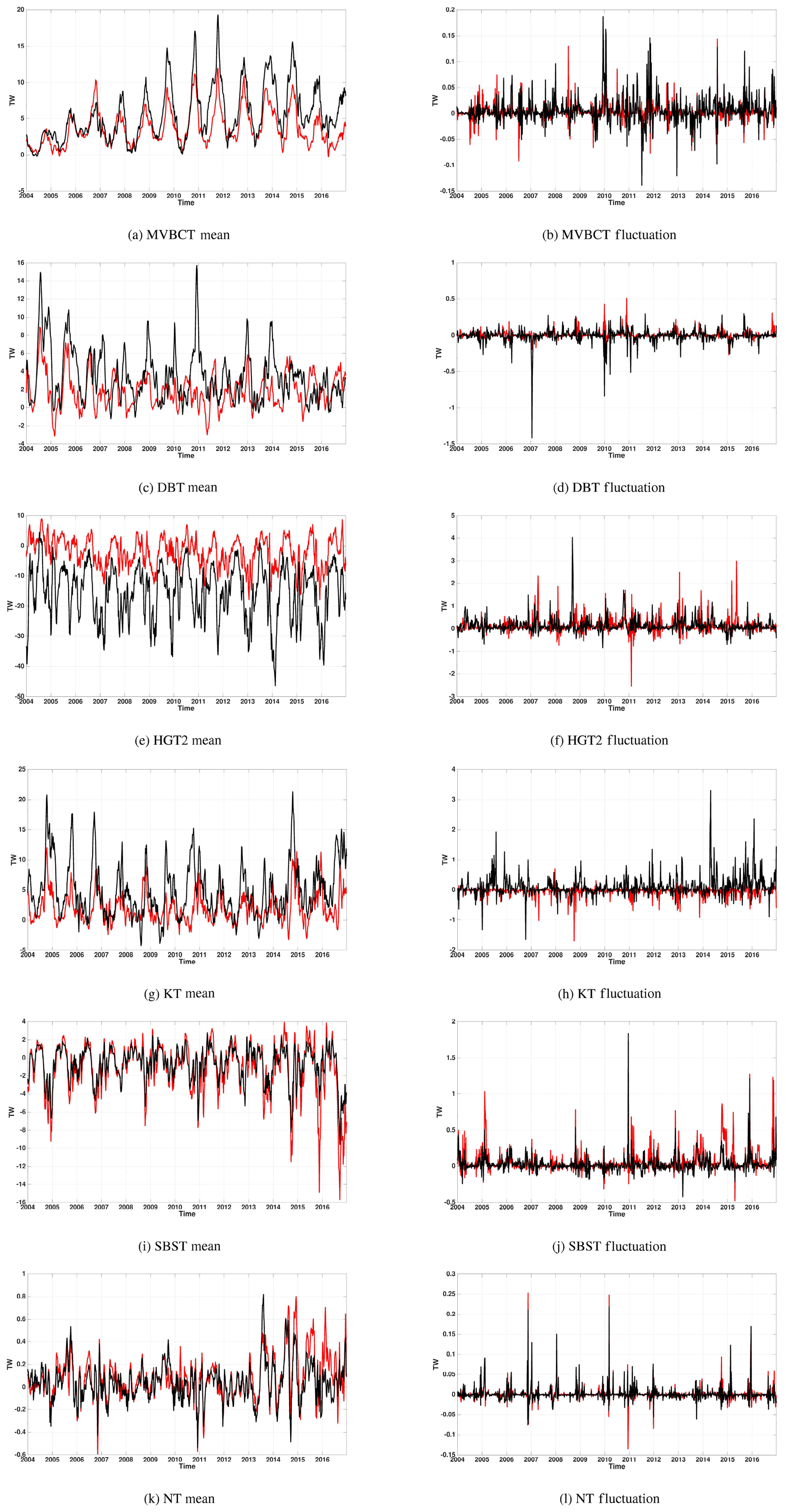
Figure 11Mean (left column) and fluctuating (right column) components of the heat flux (TW) from LowResControl (in red) and HighRes (in black). Plotted for the whole time series 2004 to 2016. Each row is for a different trough.
Warm water exchange into the troughs is very different in southeastern Greenland as compared to Baffin Bay. At HGT2, the mean heat transport in HighRes is offshore, with peak transport of −30 to −35 TW (Fig. e). The behaviour of the mean component in LowResControl is very different, with onshore heat transport reaching 10 TW in summer and autumn and balanced by offshore transport during the rest of the year. Significant differences in cross-shelf transport between 0.25 and 0.083∘ simulations were also seen by Pennelly et al. (2019). At HGT2, the fluctuation component of the heat fluxes was smaller than the mean, reaching only 2–3 TW at peaks, but is generally directed onshore (Fig. f). Thus, here at HGT2, even though the fluctuation component is relatively small compared to the mean (Table 3), the difference in directions means it plays a key role in transporting heat towards this glacier fjord. This is consistent with Christoffersen et al. (2011), who showed strong wind events were important in bringing warm waters to the coast.
For KT, the mean flow still transports the most heat, mainly in summer/autumn with peak transports reaching 16–20 TW in HighRes (substantially smaller in LowResControl) (Fig. g). However, the mean transport becomes smaller or even reverses in winter, transporting heat offshore, with maximum peaks approaching −5 TW. Meanwhile, although intermittent, the transient component of the heat flux is generally onshore in HighRes, regularly exceeding 0.5 TW and approaching 1 TW (Fig. h). This would be consistent with low-pressure systems propagating along the coast past KT, potentially linked to the Lofoten Low as suggested by Moore et al. (2014).
Moving to northeastern Greenland, SBST stood out, with the fluctuating component of the flow transporting about 76 % of the heat flux at this location (Table 3). SBST has onshore heat flux, peaking at 2–3 TW in HighRes (and only slightly different in LowResControl), associated with the mean flow (Fig. i). However, offshore heat flux peaks around −6 to −8 TW in HighRes; therefore, the heat flux direction switches from onshore to offshore. Additionally, there are occasionally strong peaks in the fluctuating component, exceeding 0.5 TW (Fig. j). There are more peaks in the fluctuating component in recent years (2011 onwards), and this might be related to the reductions in sea ice in this region or due to the presence of Pacific water on the shelf (e.g., Dmitrenko et al., 2019). The mean component dominates at NT, despite also switching between offshore and onshore directions (−0.4 to −0.8 TW in HighRes; Fig. k and l).
The correlation of the heat flux between the HighRes and LowResControl for most of the troughs was high (SBST greater than 0.9, NT and MVBCT greater than 0.8, and HGT2 greater than 0.7; see Table 3). The LowResControl and HighRes compared well with observations (see Sect. 2.4). However, since running several high-resolution experiments is computationally expensive compared to lower-resolution configurations, the LowResControl has been used for the sensitivity experiments, which will be discussed later in this paper (Sect. 3.3 and 3.4).
3.3 Impact of enhanced Greenland meltwater
Previous studies from a variety of scales of modelling have shown that enhanced freshwater discharge from the GrIS could increase the presence of heat near the ice sheet. For example, if GrIS melt increases it may add more energetic plume dynamics along a glacier face and increase the strength of the thermohaline circulation in fjords. Cai et al. (2017) showed in a 2-D model ran for 1 year, with ice shelf melt derived from observed melt rates for Petermann Glacier, that an increase in thermohaline circulation in the fjord could bring more heat and salt towards the ice sheet. Note that such fjord-scale processes are not resolved by the model simulations presented in this paper. Outside of the fjord, Castro de la Guardia et al. (2015) and Grivault et al. (2017) have found that enhanced meltwater from the GrIS could increase the heat content within Baffin Bay. Enhanced runoff decreased surface salinity in Baffin Bay, particularly along the coast. Due to the halosteric effect, it led to a lift in the sea surface height on the shelf and then an enhanced boundary current. This strengthened Baffin Bay’s cyclonic gyre in the upper layer, which resulted in a stronger Ekman pumping that lifted the isopycnals and caused the shallowing of the warm water layer in Baffin Bay. Strengthening the WGC also brought more warm waters northward into Baffin Bay. The warming and lifting of the intermediate warm layer are clearly evident in the temperature field along the western Greenland coast (Fig. ) in LowResDoubleMelt. This study provides more realistic experiments and analysis of specific locations concerning troughs that connect to fjords with large marine-terminating glaciers. With an increase in GrIS melt, Baffin Bay's ocean heat content may increase, and thus increasing the potential for glaciers to continue to melt, impacting climate, SLR, and ecosystems.

Figure 12Temperature along two sections in the northwest of Greenland, the Melville Bay section and Disko Bay section. For the location of these sections, see Fig. 1. Shown is the average temperature over the period of 2004 to 2016, with the model bathymetry in white (m) and the colours indicating the temperature of the water in ∘C. The left column (a, c) shows the results for LowResControl, and the right column (b, c) shows the results for LowResDoubleMelt. The first row (a, b) shows the Melville Bay section, and the second row (c, d) shows the Disko Bay section.
For Melville Bay in LowResControl (Fig. a), a warm core of water existed at depths 100 to 400 m, with a maximum (at the 500 km marker) in MVBST reaching almost 2 ∘C. In LowResDoubleMelt (Fig. b), the warm water core temperature increased and MVBST reached temperatures closer to 3 ∘C. The cold water layer in LowResDoubleMelt thinned more than in the LowResControl. For Disko Bay, both deep troughs (UT and DBT) held warmer water in LowResDoubleMelt (3 ∘C; Fig. d) than in LowResControl (∼2 ∘C; Fig. c). The maximum increase occurred in a warm core in both troughs, UT and DBT (at the 150 and 400 km markers), of a depth of 150 to 350 m. The cooler water layer at the surface thinned in LowResDoubleMelt (Fig. c). However, when examining average velocities normal to the section, for the entire period there was no clear trend that increasing the meltwater strengthens the velocities.
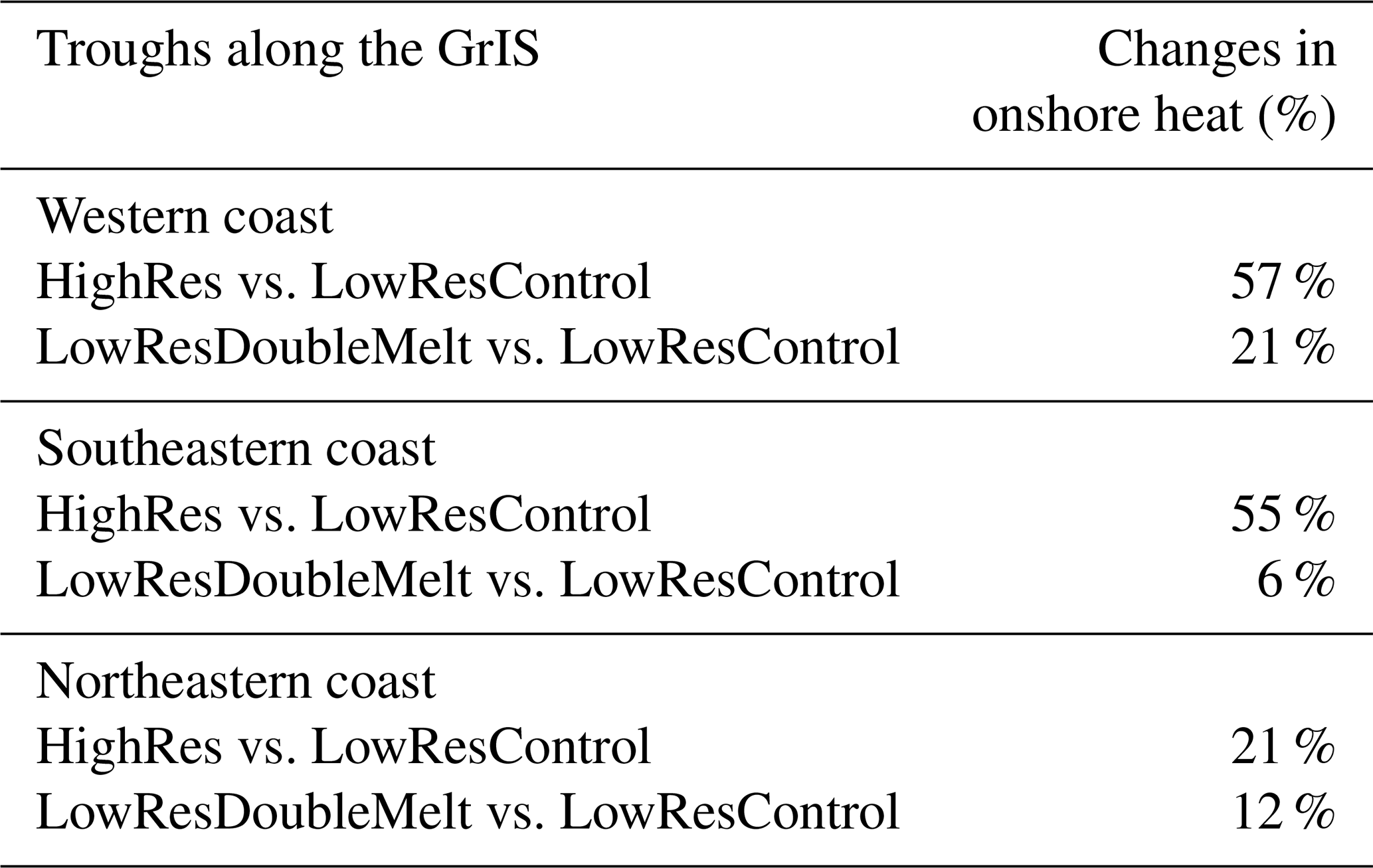
This study found that Baffin Bay was a very unique system. Other regions around Greenland did not respond to an increase in the GrIS melt in the same way. With a doubling of the meltwater, the western sector had a 21 % increase in onshore heat flux (Table 4), but we saw a 6 % decrease in the northeastern region and a 12 % decrease in the southeastern region.
Table 4This table shows the percentage of the difference between the onshore sum of yearly heat fluxes from three experiments, HighRes, LowResControl, and LowResDoubleMelt, from 2004 to 2016. The western coast includes the Melville Bay central trough (MVBCT) and Disko Bay trough (DBT), the southeastern coast sector includes Helheim Glacier trough 2 (HGT2) and Kangerlussuaq trough (KT), and the northeastern coast includes Scoresby Sund trough (SBST) and Norske trough (NT). These troughs can be identified in Fig. 1.
3.4 Impact of high-frequency atmospheric events
The question of how the atmospheric variability may impact the region of HG for renewing heat from the shelf has been discussed in previous observational studies (Straneo et al., 2010; Christoffersen et al., 2011). How does filtering out storms, where winds and the associated temperatures are impacted, affect the high frequency variability in southeastern Greenland? A comparison of LowResControl and LowResNoStorms will be shown to examine this question.
Figure 11 shows the average TKE integrated over the entire depth for the southeastern region with LowResControl and LowResNoStorms. A comparison was done for the northwestern and northeastern regions as well. However, the southeastern region had the highest TKE and the strongest sensitivity to changes in atmospheric conditions. Therefore, only the southeastern region will be shown for further analysis. LowResControl (Fig. 11a) had TKE values reaching m2 s−2. However, LowResNoStorms TKE peaked at m2 s−2, i.e., TKE is reduced by about half. Significant TKE decrease close to HGT2 is seen on the shelf at depths of less than 500 m (Fig. 11a). By filtering out storms, the TKE strength decreased in the southeastern region (Fig. 11b).
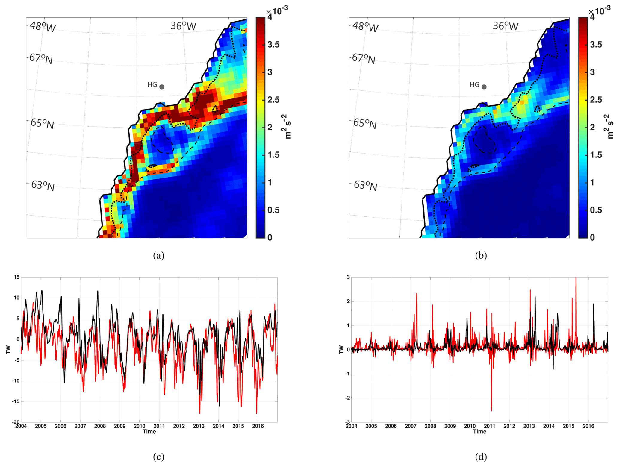
Figure 13Comparison of the filtering of the atmospheric forcing in LowResNoStorms. Panels (a) and (b) show the transient kinetic energy (TKE) integrated over the entire depth in the southeastern region of Greenland for LowResControl (a) and LowResNoStorms (b). The TKE here is the average TKE for the period of 2004 to 2016. The thick dashed lines mark the bathymetry at 250 m, and the thin dashed line marks the 500 m depth. Panel (c) shows the mean heat flux and panel (d) shows the fluctuation component of heat flux through Helheim Glacier trough 2 (HGT2) (location identified in Fig. 1). The LowResNoStorms configuration in solid black lines, and the LowResControl configuration is shown in red solid lines.
Figure 11c and d show the time series of the mean and fluctuation components of the heat flux for HGT2 with LowResControl and LowResNoStorms. The mean component has less onshore heat flux in the LowResControl than LowResNoStorms. The LowResNoStorms mean component of the onshore heat flux reached values closer to 10 TW in 2004 to the end of 2007. LowResControl had onshore heat flux values greater than 5 TW in 2004, 2007, 2010, 2015, and 2016. After 2011, both experiments have mean components that rarely surpass 5 TW and the time series show more negative (offshore direction) heat flux values. The LowResControl mean component shows more prominent offshore heat flux from 2013 to 2016, reaching maxima close to −18 TW, where LowResNoStorms has a weaker offshore mean heat flux, despite similar values with LowResControl in 2014 ( TW). The fluctuation component of the heat flux is smaller with the LowResNoStorms. The fluctuation component moderated the heat flux more with storms (21 % for the LowResControl vs. 13 % with LowResNoStorms; Table 3). Therefore, filtering storms decreased the fluctuation component of the heat flux and its control over the total heat flux.
The integration of the mean component of the heat flux from 2004 to 2016 has been calculated and compared between LowResControl and LowResNoStorms. LowResNoStorms has a total energy accumulation of 1.24 GJ (1 GJ J), where LowResControl had a total of −4.23 GJ. The total energy increase of ∼5 GJ could have the potential to melt 15 t of ice. LowResNoStorms has a 97 % increase in the onshore component of the heat for this period of 4.3 GJ compared to LowResControl (2.3 GJ). LowResNoStorms has a 52 % decrease in the offshore component of the heat for this period of −3.1 GJ compared to LowResControl (−6.4 GJ). HGT2 has more energy in the onshore direction in LowResNoStorms due to filtering out offshore winds and thus decreasing offshore heat transport. A decrease in storms decreased the offshore winds (southward), and thus there was less Ekman transport (upwelling) along the shelf. Less upwelling and offshore wind may decrease the offshore exchange of heat flux. As a result, fewer storms in this region may increase the overall onshore heat flux into HGT2.
The oceanic heat available in Greenland's troughs is dependent on the location of the trough, source of the warm water origin, how the water is transformed as it travels to the troughs, and local processes such as heat loss to the atmosphere. It is important to understand the processes that bring this warm water to the shelf and into the troughs, as this water can then be exchanged into the fjords. Warm water present in fjords provides oceanic heat forcing on marine-terminating glaciers (Rignot et al., 2016b; Cai et al., 2017; Wood et al., 2018). To our knowledge, this is the first study looking at seasonal changes in heat flux in troughs that are connected to fjords with marine-terminating glaciers.
This study showed that the presence of warm water at depth can extend far north into Baffin Bay, reaching as north as Melville Bay and its subsequent troughs. Increased heat flux through the Melville Bay section is found from 2009 to the end of 2014. Therefore an associated increase in ocean heat presence in these troughs may have driven more heat to glaciers that terminate there. From 2004 to 2006, model experiments captured an increase in onshore heat flux in DBT, coinciding with the timing of the disintegration of JI floating tongue and within the period of observed oceanic heat increase in Disko Bay (from 1997 to 2007) (Holland et al., 2008).
The seasonality of the maximum onshore heat flux through all six regions has been presented in this paper.
This study looked at heat fluxes using a reference temperature of −1.5 ∘C to consider the effects of boundary layer salinity and pressure on the freezing point (see Sect. 2.3 for further detail). Therefore, the heat present in the troughs that we consider is not simply modified Irminger Water (although that will be the most important component off western Greenland). The seasonality of the maximum onshore heat flux through troughs around the GrIS differs as the distance between the Irminger Sea increases. Therefore, the influence of the Irminger Current may still present itself in these troughs and other warm waters. The seasonal peak of warm waters began in June for HGT2, in July for DBT, and in September for MVBCT. Then for the areas receiving warm water from the NwAC this began in August for KT, in November for SBS, and from September to January for NT.
The southeastern region had the highest TKE and the strongest sensitivity to changes in atmospheric conditions. The southeastern coast of Greenland is impacted the most by the atmospheric filter (i.e., no storms). No storms resulted in a reduction of TKE (∼50 %), less offshore heat transport, and more onshore heat flux (97 %) through the Helheim Glacier trough 2 (HGT2).
It is imperative to try to understand how sensitive the ocean is to additional meltwater from Greenland. Baffin Bay is a unique system, as it responded to an increase in the GrIS melt in a different way to any other region around Greenland in this study. Troughs off the western coast of Greenland in Baffin Bay brought more heat (∼20 %) towards the GrIS when the GrIS freshwater flux doubled. This study showed that a doubling of the GrIS melt may cause warming in Baffin Bay and an increase in heat flux through troughs, potentially escalating the melt of the GrIS, consistent with Castro de la Guardia et al. (2015), but now in a more realistic setup with Greenland meltwater temporally and spatially distributed.
Since the model used in this study cannot resolve small-scale processes such as fjord circulation, the exchange between fjords and troughs cannot be looked into. Instead, there is an assumption in place that the water characteristics that exist in the troughs will match those in the fjords due to the dynamics of cross-shelf exchanges (Jackson et al., 2014; Sutherland et al., 2014). Warming of ocean water in troughs may lead to a warming of ocean waters in fjords. Due to the model bathymetry under-representing the depth of these troughs, this study may be underestimating the amount of ocean heat available to enter these troughs. The study only looked at the impact of the freshwater flux from the GrIS. The inclusion of an iceberg model coupled with an ocean model (Marson et al., 2018) may give further insight into the heat and freshwater budget in regions of high GrIS discharge.
The model code based on the NEMO model is available at https://www.nemo-ocean.eu/ (last access: 28 May 2017, Madec, 2008). Details on the ANHA configuration used are available at http://knossos.eas.ualberta.ca/anha/index.php (last access: 8 September 2017), with files for the reference experiment at https://doi.org/10.7939/DVN/GIXGXB (Hu, 2020).
Observations from the mooring array at Davis Strait (e.g., Curry et al., 2011, 2014) are available online for download at http://iop.apl.washington.edu/data.php (last access: 31 August 2016).
LCG and PGM designed the study, and LCG carried it out. XH developed the model configuration and performed the simulations. LCG prepared the manuscript with contributions from all co-authors. MHR and CL provided comments on the manuscript, with CL also providing Davis Strait data.
The authors declare that they have no conflict of interest.
We would like to thank Yarisbel Garcia-Quintana for carrying out the LowResNoStorm experiment. We are grateful to the NEMO development team and the Drakkar project for providing the model and continuous guidance and to Westgrid and Compute Canada for computational resources, where all model experiments were performed and archived (http://www.computecanada.ca; last access: 16 August 2017). The authors would like to thank the anonymous reviewers for their insightful comments and suggestions that have contributed to improving this paper.
This research has been supported by the Natural Sciences and Engineering Research Council of Canada (grant nos. rgpin227438, rgpcc433898, and 432295).
This paper was edited by Dirk Notz and reviewed by two anonymous referees.
Aagaard, K. and Carmack, E. C.: The role of sea ice and other fresh water in the Arctic circulation, J. Geophys. Res.-Oceans, 94, 14 485–14 498, https://doi.org/10.1029/JC094iC10p14485, 1989. a
Aksenov, Y., Bacon, S., Coward, A. C., and Holliday, N. P.: Polar outflow from the Arctic Ocean: A high resolution model study, J. Marine Sys., 83, 14–37, https://doi.org/10.1016/j.jmarsys.2010.06.007, 2010. a
Amante, C. and Eakins, B.: ETOPO1 1 Arc-Minute Global Relief Model: Procedures, Data Sources and Analysis, NOAA Technical Memorandum NESDIS NGDC-24, https://doi.org/10.7289/V5C8276M, 2009. a, b
An, L., Rignot, E., Elieff, S., Morlighem, M., Millan, R., Mouginot, J., Holland, D. M., Holland, D., and Paden, J.: Bed elevation of Jakobshavn Isbrae, West Greenland, from high-resolution airborne gravity and other data, Geophys. Res. Lett., 44, 3728–3736, https://doi.org/10.1002/2017GL073245, 2017. a, b
Arrigo, K. R., van Dijken, G. L., Castelao, R. M., Luo, H., Rennermalm, s. K., Tedesco, M., Mote, T. L., Oliver, H., and Yager, P. L.: Melting glaciers stimulate large summer phytoplankton blooms in southwest Greenland waters, Geophys. Res. Lett., 44, 6278–6285, https://doi.org/10.1002/2017GL073583, 2017. a
Azetsu-Scott, K. and Tan, F. C.: Oxygen isotope studies from Iceland to an East Greenland Fjord: behaviour of glacial meltwater plume, Mar. Chem., 56, 239–251, https://doi.org/10.1016/S0304-4203(96)00078-3, 1997. a, b
Bacon, S., Marshall, A., Holliday, N. P., Aksenov, Y., and Dye, S. R.: Seasonal variability of the East Greenland Coastal Current, J. Geophys. Res.-Oceans, 119, 3967–3987, https://doi.org/10.1002/2013JC009279, 2014. a
Bamber, J., Van Den Broeke, M., Ettema, J., Lenaerts, J., and Rignot, E.: Recent large increases in freshwater fluxes from Greenland into the North Atlantic, Geophys. Res. Lett., 39, L19501, https://doi.org/10.1029/2012GL052552, 2012. a, b, c
Bamber, J. L., Griggs, J. A., Hurkmans, R. T. W. L., Dowdeswell, J. A., Gogineni, S. P., Howat, I., Mouginot, J., Paden, J., Palmer, S., Rignot, E., and Steinhage, D.: A new bed elevation dataset for Greenland, The Cryosphere, 7, 499–510, https://doi.org/10.5194/tc-7-499-2013, 2013. a
Barnier, B., Brodeau, L., Le Sommer, J., Molines, J., Penduff, T., Theetten, S., Treguier, A. M., Madec, G., Biastoch, A., Böning, C., Dengg, J., Gulev, S., Bourdallé, B. R., Chanut, J., Garric, G., Alderson, S., Coward, A., de Cuevas, B., New, A., Haines, K., Smith, G., Drijfhout, S., Hazeleger, W., Severijns, C., and Myers, P.: Eddy-permitting ocean circulation hindcasts of past decades, CLIVAR Exchanges, 12, 8–10, 2007. a, b, c
Bartholomaus, T. C., Stearns, L. A., Sutherland, D. A., Shroyer, E. L., Nash, J. D., Walker, R. T., Catania, G., Felikson, D., Carroll, D., Fried, M. J., Noël, B. P. Y., and Van Den Broeke, M. R.: Contrasts in the response of adjacent fjords and glaciers to ice-sheet surface melt in West Greenland, Ann. Glaciol., 57, 25–38, https://doi.org/10.1017/aog.2016.19, 2016. a
Beaird, N., Straneo, F., and Jenkins, W.: Characteristics of meltwater export from Jakobshavn Isbræ and Ilulissat Icefjord, Ann. Glaciol., 58, 107–117, https://doi.org/10.1017/aog.2017.19, 2017. a
Beaird, N. L., Straneo, F., and Jenkins, W.: Export of Strongly Diluted Greenland Meltwater From a Major Glacial Fjord, Geophys. Res. Lett., 45, 4163–4170, https://doi.org/10.1029/2018GL077000, 2018. a
Bernard, B., Madec, G., Penduff, T., Molines, J.-M., Treguier, A.-M., Le Sommer, J., Beckmann, A., Biastoch, A., Böning, C., Dengg, J., Derval, C., Durand, E., Gulev, S., Remy, E., Talandier, C., Theetten, S., Maltrud, M., McClean, J., and De Cuevas, B.: Impact of partial steps and momentum advection schemes in a global ocean circulation model at eddy-permitting resolution, Ocean Dynam., 56, 543–567, https://doi.org/10.1007/s10236-006-0082-1, 2006. a
Beszczynska-Möller, A., Fahrbach, E., Schauer, U., and Hansen, E.: Variability in Atlantic water temperature and transport at the entrance to the Arctic Ocean, 1997–2010, ICES J. Mar. Sci., 69, 852–863, https://doi.org/10.1093/icesjms/fss056, 2012. a, b, c
BODC: British Oceanographic Data Center's General Bathymetric Chart of the Oceans, available at: http://blog.bodc.ac.uk/2008/ (last access: 9 March 2017), 2008. a
Böning, C. W., Behrens, E., Biastoch, A., Getzlaff, K., and Bamber, J. L.: Emerging impact of Greenland meltwater on deepwater formation in the North Atlantic Ocean, Nature Geosci., 9, 523–527, https://doi.org/10.1038/ngeo2740, 2016. a, b, c
Box, J. E.and Yang, L., Bromwich, D. H., and Bai, L.: Greenland Ice Sheet Surface Air Temperature Variability: 1840–2007, J. Climate, 22, 4029–4049, https://doi.org/10.1175/2009JCLI2816.1, 2009. a
Cai, C., Rignot, E., Menemenlis, D., and Nakayama, Y.: Observations and modeling of ocean-induced melt beneath Petermann Glacier Ice Shelf in northwestern Greenland, Geophys. Res. Lett., 44, 8396–8403, https://doi.org/10.1002/2017GL073711, 2017. a, b, c, d
Castro de la Guardia, L., Hu, X., and Myers, P. G.: Potential positive feedback between Greenland Ice Sheet melt and Baffin Bay heat content on the west Greenland shelf, Geophys. Res. Lett., 42, 4922–4930, https://doi.org/10.1002/2015GL064626, 2015. a, b, c, d
Christoffersen, P., Mugford, R. I., Heywood, K. J., Joughin, I., Dowdeswell, J. A., Syvitski, J. P. M., Luckman, A., and Benham, T. J.: Warming of waters in an East Greenland fjord prior to glacier retreat: mechanisms and connection to large-scale atmospheric conditions, The Cryosphere, 5, 701–714, https://doi.org/10.5194/tc-5-701-2011, 2011. a, b, c, d
Csatho, B. M., Schenk, A. F., van der Veen, C. J., Babonis, G., Duncan, K., Rezvanbehbahani, S., van den Broeke, M. R., Simonsen, S. B., Nagarajan, S., and van Angelen, J. H.: Laser altimetry reveals complex pattern of Greenland Ice Sheet dynamics, P. Natl. Acad. Sci. USA., 111, 18 478–18 483, https://doi.org/10.1073/pnas.1411680112, 2014. a
Curry, B., Lee, C. M., and Petrie, B.: Volume, Freshwater, and Heat Fluxes through Davis Strait, 2004–05, J. Phys. Oceanogr., 41, 429–436, https://doi.org/10.1175/2010JPO4536.1, 2011. a, b, c, d, e, f, g
Curry, B., Lee, C., Petrie, B., Moritz, R., and Kwok, R.: Multiyear volume, liquid freshwater, and sea ice transports through Davis Strait, 2004–10, J. Phys. Oceanogr., 44, 1244–1266, https://doi.org/10.1175/JPO-D-13-0177.1, 2014. a, b, c, d, e, f, g, h, i
Dai, A., Qian, T., Trenberth, K. E., and Milliman, J. D.: Changes in continental freshwater discharge from 1948 to 2004, J. Climate, 22, 2773–2792, 2009. a, b
Dmitrenko, I. A., Kirillov, S. A., Rudels, B., Babb, D. G., Myers, P. G., Stedmon, C. A., Bendtsen, J., Ehn, J. K., Pedersen, L. T., Rysgaard, S., and Barber, D. G.: Variability of the Pacific-Derived Arctic Water Over the Southeastern Wandel Sea Shelf (Northeast Greenland) in 2015–2016, J. Geophys. Res.-Oceans, 124, 349–373, https://doi.org/10.1029/2018JC014567, 2019. a
Dukhovskoy, D. S., Myers, P. G., Platov, G., Timmermans, M.-L., Curry, B., Proshutinsky, A., Bamber, J. L., Chassignet, E., Hu, X., Lee, C. M., and Somavilla, R.: Greenland freshwater pathways in the sub-Arctic Seas from model experiments with passive tracers, J. Geophys. Res.-Oceans, 121, 877–907, https://doi.org/10.1002/2015JC011290, 2016. a, b
Eskridge, R. E., Ku, J. Y., Rao, S. T., Porter, P. S., and Zurbenko, I. G.: Separating Different Scales of Motion in Time Series of Meteorological Variables, B. Am. Meteorol. Soc., 78, 1473–1484, https://doi.org/10.1175/1520-0477(1997)078<1473:SDSOMI>2.0.CO;2, 1997. a, b
Felikson, D., Bartholomaus, T. C., Catania, G. A., Korsgaard, N. J., Kjær, K. H., Morlighem, M., Noël, B., van den Broeke, M., Stearns, L. A., Shroyer, E. L., Sutherland, D. A., and Nash, J. D.: Inland thinning on the Greenland Ice Sheet controlled by outlet glacier geometry, Nat. Geosci., 10, 36–369, https://doi.org/10.1038/ngeo2934, 2017. a
Fenty, I., Willis, J. K., Khazendar, A., Dinardo, S., Forsberg, R., Fukumori, I., Holland, D., Jakobsson, M., Moller, D., Münchow, J. M. A., Rignot, E., Schodlok, M., Thompson, A. F., Tinto, K., Rutherford, M., and Trenholm, N.: Oceans Melting Greenland: Early Results from NASA’s Ocean-Ice Mission in Greenland , Oceanography, 29, 72–83, https://doi.org/10.5670/oceanog.2016.100, 2016. a
Ferry, N., Greiner, E., Garric, G., Penduff, T., Treiguier, A.-M., and Reverdin, G.: GLORYS-1 Reference Manual for Stream 1 (2002–2007), GLORYS project report, available at: https://marine.copernicus.eu/ (last accessed: 10 February 2014), 2008. a
Fichefet, T. and Morales Maqueda, M.: Sensitivity of a global sea ice model to the treatment of ice thermodynamics and dynamics, J. Geophys. Res., 102, 12 609–12 646, 1997. a
Fratantoni, P. S. and Pickart, R. S.: The western North Atlantic shelfbreak current system in summer, J. Phys. Oceanogr., 37, 2509–2533, 2007. a
Garcia-Quintana, Y., Courtois, P., Hu, X., Pennelly, C., Kieke, D., and Myers, P. G.: Sensitivity of Labrador Sea Water Formation to Changes in Model Resolution, Atmospheric Forcing, and Freshwater Input, J. Geophys. Res.-Oceans, 124, 2126–2152, https://doi.org/10.1029/2018JC014459, 2019. a, b
Gillard, L. C., Hu, X., Myers, P. G., and Bamber, J. L.: Meltwater pathways from marine terminating glaciers of the Greenland Ice Sheet, Geophys. Res. Lett., 43, 10,873–10,882, https://doi.org/10.1002/2016GL070969, 2016. a
Gladish, C., Holland, D., and Lee, C.: Oceanic boundary conditions for Jakobshavn Glacier. Part II: Provenance and sources of variability of disko bay and Ilulissat Icefjord waters, 1990–2011, J. Phys. Oceanogr., 45, 33–63, https://doi.org/10.1175/JPO-D-14-0045.1, 2015a. a, b
Gladish, C., Holland, D., Rosing-Asvid, A., Behrens, J., and Boje, J.: Oceanic boundary conditions for Jakobshavn Glacier. Part I: Variability and renewal of Ilulissat Icefjord waters, 2001-14, J. Phys. Oceanogr., 45, 3–32, https://doi.org/10.1175/JPO-D-14-0044.1, 2015b. a
Grist, J. P., Josey, S. A., Boehme, L., Meredith, M. P., Laidre, K. L., Heide-Jørgensen, M. P., Kovacs, K. M., Lydersen, C., Davidson, F. J. M., Stenson, G. B., Hammill, M. O., Marsh, R., and Coward, A. C.: Seasonal variability of the warm Atlantic water layer in the vicinity of the Greenland shelf break, Geophys. Res. Lett., 41, 8530–8537, https://doi.org/10.1002/2014GL062051, 2014. a, b, c, d
Grivault, N., Hu, X., and Myers, P. G.: Evolution of Baffin Bay Water Masses and Transports in a Numerical Sensitivity Experiment under Enhanced Greenland Melt, Atmos. Ocean, 55, 169–194, https://doi.org/10.1080/07055900.2017.1333950, 2017. a
Hogan, K. A., Cofaigh, C., Jennings, A. E., Dowdeswell, J. A., and Hiemstra, J. F.: Deglaciation of a major palaeo-ice stream in Disko Trough, West Greenland, Quaternary Sci. Rev., 147, 5–26, https://doi.org/10.1016/j.quascirev.2016.01.018, 2016. a
Holdsworth, A. M. and Myers, P. G.: The Influence of High-Frequency Atmospheric Forcing on the Circulation and Deep Convection of the Labrador Sea, J. Climate, 28, 4980–4996, https://doi.org/10.1175/JCLI-D-14-00564.1, 2015. a
Holland, D. M. and Jenkins, A.: Modeling Thermodynamic Ice–Ocean Interactions at the Base of an Ice Shelf, J. Phys. Oceanogr., 29, 1787–1800, https://doi.org/10.1175/1520-0485(1999)029<1787:MTIOIA>2.0.CO;2, 1999. a
Holland, D. M., Thomas, R. H., De Young, B., Ribergaard, M. H., and Lyberth, B.: Acceleration of Jakobshavn Isbrae triggered by warm subsurface ocean waters, Nat. Geosci., 1, 659–664, 2008. a, b, c, d, e, f
Hu, X.: ANHA4-EXH005, V1, UAL Dataverse, https://doi.org/10.7939/DVN/GIXGXB, 2020. a
Hu, X. and Myers, P. G.: A Lagrangian view of Pacific water inflow pathways in the Arctic Ocean during model spin-up, Ocean Model., 71, 66–80, https://doi.org/10.1016/j.ocemod.2013.06.007, 2013. a, b, c
Inall, M. E., Murray, T., Cottier, F. R., Scharrer, K., Boyd, T. J., Heywood, K. J., and Bevan, S. L.: Oceanic heat delivery via Kangerdlugssuaq Fjord to the south-east Greenland Ice Sheet, J. Geophys. Res.-Oceans, 119, 631–645, https://doi.org/10.1002/2013JC009295, 2014. a
Jackson, R. H., Straneo, F., and Sutherland, D. A.: Externally forced fluctuations in ocean temperature at Greenland glaciers in non-summer months, Nat. Geosci., 7, 503–508, 2014. a, b, c, d
Jenkins, A.: Convection-driven melting near the grounding lines of ice shelves and tidewater glaciers, J. Phys. Oceanogr., 41, 2279–2294, 2011. a
Joughin, I., Alley, R. B., and Holland, D. M.: Ice-Sheet Response to Oceanic Forcing, Science, 338, 1172–1176, https://doi.org/10.1126/science.1226481, 2012. a
Karcher, M., Beszczynska-Möller, A., Kauker, F., Gerdes, R., Heyen, S., Rudels, B., and Schauer, U.: Arctic Ocean warming and its consequences for the Denmark Strait overflow, J. Geophys. Res.-Oceans, 116, C02037, https://doi.org/10.1029/2010JC006265, 2011. a
Khazendar, A., Fenty, I. G., Carroll, D., Gardner, A. an Lee, C. M., Fukumori, I., Wang, O., Zhang, H., Seroussi, H., Moller, D., Noël, B. P. Y., van den Broeke, M. R., Dinardo, S., and Willis, J.: Interruption of two decades of Jakobshavn Isbrae acceleration and thinning as regional ocean cools, Nat. Geosci., 12, 277–283, https://doi.org/10.1038/s41561-019-0329-3, 2019. a
Luo, H., Castelao, R. M., Rennermalm, A. K., Tedesco, M., Bracco, A., Yager, P. L., and Mote, T. L.: Oceanic transport of surface meltwater from the southern Greenland Ice Sheet, Nat. Geosci., 9, 528–532, https://doi.org/10.1038/ngeo2708, 2016. a
Madec, G.: NEMO ocean engine, Note du Pole de modélisation, https://www.nemo-ocean.eu/doc/ (last access: 28 May 2017), 2008. a, b
Marson, J. M., Myers, P. G., Hu, X., and Le Sommer, J.: Using Vertically Integrated Ocean Fields to Characterize Greenland Icebergs' Distribution and Lifetime, Geophys. Res. Lett., 45, 4208–4217, https://doi.org/10.1029/2018GL077676, 2018. a
Mayer, C., Reeh, N., Jung-Rothenhäusler, F., Huybrechts, P., and Oerter, H.: The subglacial cavity and implied dynamics under Nioghalvfjerdsfjorden Glacier, NE-Greenland, Geophys. Res. Lett., 27, 2289–2292, https://doi.org/10.1029/2000GL011514, 2000. a
MEOM: Bathymetry ORCA0.25, available at: http://servdap.legi.grenoble-inp.fr/meom/ORCA025-I/ (last accessed: 5 March 2015), 2013. a
Moon, T., Joughin, I., and Smith, B.: Seasonal to multiyear variability of glacier surface velocity, terminus position, and sea ice/ice mélange in northwest Greenland, J. Geophys. Res.-Earth, 120, 818–833, https://doi.org/10.1002/2015JF003494, 2015. a
Moore, G. W. K., Straneo, F., and Oltmanns, M.: Trend and interannual variability in southeast Greenland Sea Ice: Impacts on coastal Greenland climate variability, Geophys. Res. Lett., 41, 8619–8626, https://doi.org/10.1002/2014GL062107, 2014. a
Morlighem, M., Williams, C. N., Rignot, E., An, L., Arndt, J. E., Bamber, J. L., Catania, G., Chauché, N., Dowdeswell, J. A., Dorschel, B., Fenty, I., Hogan, K., Howat, I., Hubbard, A., Jakobsson, M., Jordan, T. M., Kjeldsen, K. K., Millan, R., Mayer, L., Mouginot, J., Noël, B. P. Y., O'Cofaigh, C., Palmer, S., Rysgaard, S., Seroussi, H., Siegert, M. J., Slabon, P., Straneo, F., van den Broeke, M. R., Weinrebe, W., Wood, M., and Zinglersen, K. B.: BedMachine v3: Complete Bed Topography and Ocean Bathymetry Mapping of Greenland From Multibeam Echo Sounding Combined With Mass Conservation, Geophys. Res. Lett., 44, 11,051–11,061, https://doi.org/10.1002/2017GL074954, 2017. a, b, c, d, e, f
Myers, P. G. and Ribergaard, M. H.: Warming of the polar water layer in Disko Bay and potential impact on Jakobshavn Isbrae, J. Phys. Oceanogr., 43, 2629–2640, 2013. a, b, c
Myers, P. G., Donnelly, C., and Ribergaard, M. H.: Structure and variability of the West Greenland Current in Summer derived from 6 repeat standard sections, Prog. Oceanogr., 80, 93–112, 2009. a
National Geophysical Data Centre: 2-minute Gridded Global Relief Data (ETOPO2) v2., National Geophysical Data Center, NOAA, https://doi.org/10.7289/V5J1012Q (last accessed: 09 May 2017), 2006. a
Pennelly, C., Hu, X., and Myers, P. G.: Cross-Isobath Freshwater Exchange Within the North Atlantic Subpolar Gyre, J. Geophys. Res.-Oceans, 124, 6831–6853, https://doi.org/10.1029/2019JC015144, 2019. a
Porter, D. F., Tinto, K. J., Boghosian, A., Cochran, J. R., Bell, R. E., Manizade, S. S., and Sonntag, J. G.: Bathymetric control of tidewater glacier mass loss in northwest Greenland, Earth Planet. Sc. Lett., 401, 40–46, https://doi.org/10.1016/j.epsl.2014.05.058, 2014. a
Rastner, P., Bolch, T., Mölg, N., Machguth, H., Le Bris, R., and Paul, F.: The first complete inventory of the local glaciers and ice caps on Greenland, The Cryosphere, 6, 1483–1495, https://doi.org/10.5194/tc-6-1483-2012, 2012. a, b
Ribergaard, M.: Oceanographic Investigations off West Greenland 2013, NAFO Scientific Council Documents, available online at: http://ocean.dmi.dk/staff/mhri/Docs/scr14-001.pdf (last access: 21 August 2020), 2014. a, b, c, d
Rignot, E. and Kanagaratnam, P.: Changes in the velocity structure of the Greenland Ice Sheet, Science, 311, 986–990, 2006. a, b
Rignot, E. and Mouginot, J.: Ice flow in Greenland for the International Polar Year 2008-2009, Geophys. Res. Lett., 39, L11501, https://doi.org/10.1029/2012GL051634, 2012. a, b
Rignot, E., Fenty, I., Xu, Y., Cai, C., Velicogna, I., Cofaigh, C. ., Dowdeswell, J. A., Weinrebe, W., Catania, G., and Duncan, D.: Bathymetry data reveal glaciers vulnerable to ice-ocean interaction in Uummannaq and Vaigat glacial fjords, west Greenland, Geophys. Res. Lett., 43, 2667–2674, https://doi.org/10.1002/2016GL067832, 2016a. a
Rignot, E., Xu, Y., Menemenlis, D., Mouginot, J., Scheuchl, B., Li, X., Morlighem, M., Seroussi, H., den Broeke, M. v., Fenty, I., Cai, C., An, L., and Fleurian, B. d.: Modeling of ocean-induced ice melt rates of five west Greenland glaciers over the past two decades, Geophys. Res. Lett., 43, 6374–6382, https://doi.org/10.1002/2016GL068784, 2016b. a, b
Schaffer, J., von Appen, W.-J., Dodd, P. A., Hofstede, C., Mayer, C., de Steur, L., and Kanzow, T.: Warm water pathways toward Nioghalvfjerdsfjorden Glacier, Northeast Greenland, J. Geophys. Res.-Oceans, 122, 4004–4020, https://doi.org/10.1002/2016JC012462, 2017. a
Seroussi, H., Morlighem, M., Rignot, E., Larour, E., Aubry, D., Ben Dhia, H., and Kristensen, S. S.: Ice flux divergence anomalies on 79north Glacier, Greenland, Geophys. Res. Lett., 38, L09501, https://doi.org/10.1029/2011GL047338, 2011. a
Slabon, P., Dorschel, B., Jokat, W., Myklebust, R., Hebbeln, D., and Gebhardt, C.: Greenland ice sheet retreat history in the northeast Baffin Bay based on high-resolution bathymetry, Quaternary Sci. Rev., 154, 182–198, https://doi.org/10.1016/j.quascirev.2016.10.022, 2016. a
Smith, G. C., Roy, F., Mann, P., Dupont, F., Brasnett, B., Lemieux, J.-F., Laroche, S., and Bélair, S.: A new atmospheric dataset for forcing ice-ocean models: Evaluation of reforecasts using the Canadian global deterministic prediction system, Q. J. Roy. Meteor. Soc., 140, 881–894, 2014. a, b
Smith, W. H. F. and Sandwell, D. T.: Global seafloor topography from satellite altimetry and ship depth soundings, Science, 277, 1957–1962, 1997. a
Straneo, F.: Heat and freshwater transport through the central Labrador Sea, J. Phys. Oceanogr., 36, 606–628, 2006. a
Straneo, F. and Heimbach, P.: North Atlantic warming and the retreat of Greenland's outlet glaciers, Nature, 504, 36–43, 2013. a, b
Straneo, F., Hamilton, G., Sutherland, D., Stearns, L. A., Davidson, F., Hammill, M., Stenson, G. B., and A., R.: Rapid circulation of warm subtropical waters in a major glacial fjord in East Greenland, Nat. Geosci., 3, 182–186, 2010. a, b, c
Straneo, F., Sutherland, D. A., Holland, D., Gladish, C., Hamilton, G. S., Johnson, H. L., Rignot, E., Xu, Y., and Koppes, M.: Characteristics of ocean waters reaching Greenland's glaciers, Ann. Glaciol., 53, 202–210, 2012. a, b
Sutherland, D. A., Straneo, F., and Pickart, R. S.: Characteristics and dynamics of two major Greenland glacial fjords, J. Geophys. Res.-Oceans, 119, 3767–3791, 2014. a
Swingedouw, D., Rodehacke, C. B., Olsen, S. M., Menary, M., Gao, Y., Mikolajewicz, U., and Mignot, J.: On the reduced sensitivity of the Atlantic overturning to Greenland Ice Sheet melting in projections: a multi-model assessment, Clim. Dynam., 2014. a
van den Broeke, M. R., Enderlin, E. M., Howat, I. M., Kuipers Munneke, P., Noël, B. P. Y., van de Berg, W. J., van Meijgaard, E., and Wouters, B.: On the recent contribution of the Greenland ice sheet to sea level change, The Cryosphere, 10, 1933–1946, https://doi.org/10.5194/tc-10-1933-2016, 2016. a, b, c
Weijer, W., Maltrud, M. E., Hecht, M. W., Dijkstra, H. A., and Kliphuis, M. A.: Response of the Atlantic Ocean circulation to Greenland Ice Sheet melting in a strongly-eddying ocean model, Geophys. Res. Lett., 39, L09606, https://doi.org/10.1029/2012GL051611, 2012. a, b, c
Williams, C. N., Cornford, S. L., Jordan, T. M., Dowdeswell, J. A., Siegert, M. J., Clark, C. D., Swift, D. A., Sole, A., Fenty, I., and Bamber, J. L.: Generating synthetic fjord bathymetry for coastal Greenland, The Cryosphere, 11, 363–380, https://doi.org/10.5194/tc-11-363-2017, 2017. a
Wilson, N. J. and Straneo, F.: Water exchange between the continental shelf and the cavity beneath Nioghalvfjerdsbrae (79 North Glacier), Geophys. Res. Lett., 42, 7648–7654, https://doi.org/10.1002/2015GL064944, 2015. a, b, c, d
Wood, M., Rignot, E., Fenty, I., Menemenlis, D., Millan, R., Morlighem, M., Mouginot, J., and Seroussi, H.: Ocean-Induced Melt Triggers Glacier Retreat in Northwest Greenland, Geophys. Res. Lett., 45, 8334–8342, https://doi.org/10.1029/2018GL078024, 2018. a, b, c
Zurbenko, I., Porter, P. S., Gui, R., Rao, S. T., Ku, J. Y., and Eskridge, R. E.: Detecting Discontinuities in Time Series of Upper-Air Data: Development and Demonstration of an Adaptive Filter Technique, J. Climate, 9, 3548–3560, https://doi.org/10.1175/1520-0442(1996)009<3548:DDITSO>2.0.CO;2, 1996. a, b