Clouds damp the radiative impacts of polar sea ice loss

Clouds play an important role in the climate system: (1) cooling Earth by reflecting incoming sunlight to space and (2) warming Earth by reducing thermal energy loss to space. Cloud radiative effects are especially important in polar regions and have the potential to significantly alter the impact of sea ice decline on the surface radiation budget. Using CERES (Clouds and the Earth's Radiant Energy System) data and 32 CMIP5 (Coupled Model Intercomparison Project) climate models, we quantify the influence of polar clouds on the radiative impact of polar sea ice variability. Our results show that the cloud short-wave cooling effect strongly influences the impact of sea ice variability on the surface radiation budget and does so in a counter-intuitive manner over the polar seas: years with less sea ice and a larger net surface radiative flux show a more negative cloud radiative effect. Our results indicate that 66±2% of this change in the net cloud radiative effect is due to the reduction in surface albedo and that the remaining 34±1 % is due to an increase in cloud cover and optical thickness. The overall cloud radiative damping effect is 56±2 % over the Antarctic and 47±3 % over the Arctic. Thus, present-day cloud properties significantly reduce the net radiative impact of sea ice loss on the Arctic and Antarctic surface radiation budgets. As a result, climate models must accurately represent present-day polar cloud properties in order to capture the surface radiation budget impact of polar sea ice loss and thus the surface albedo feedback.

1 Introduction

Solar radiation is the primary energy source for the Earth system and provides the energy driving motions in the atmosphere and ocean, the energy behind water phase changes, and the energy stored in fossil fuels. Only a fraction (Loeb et al., 2018) of the solar energy arriving to the top of the Earth atmosphere (short-wave radiation; SW) is absorbed at the surface. Some of it is reflected back to space by clouds and by the surface, while some is absorbed by the atmosphere. In parallel, Earth's surface and atmosphere emit thermal energy back to space, called outgoing long-wave (LW) radiation, resulting in a loss of energy (Fig. 1). The balance between these energy exchanges determines Earth's present and future climate. The change in this balance is particularly important over the Arctic, where summer sea ice is retreating at an accelerated rate (Comiso et al., 2008), surface albedo is rapidly declining and surface temperatures are rising at a rate double that of the global average (Cohen et al., 2014; Graversen et al., 2008), impacting sub-polar ecosystems (Cheung et al., 2009; Post et al., 2013) and possibly mid-latitude climate (Cohen et al., 2014, 2019).

Clouds play an important role in modifying the radiative energy flows that determine Earth's climate. This is done both by increasing the amount of SW reflected back to space and by reducing the LW energy loss to space relative to clear skies (Fig. 1). These cloud effects on Earth's radiation budget can be gauged using the cloud radiative effect (CRE), defined as the difference between the actual atmosphere and the same atmosphere without clouds (Charlock and Ramanathan, 1985). The different spectral components of this effect can be estimated from satellite observations: the global average SW cloud radiative effect (SW_cre) is negative, since clouds reflect incoming solar radiation back to space, resulting in a cooling effect. On the other hand, the LW cloud radiative effect (LW_cre) is positive, since clouds reduce the outgoing LW radiation to space generating a warming effect (Harrison et al., 1990; Loeb et al., 2018; Ramanathan et al., 1989). Cloud properties and their radiative effects exhibit significant uncertainty in the polar regions (e.g. Curry et al., 1996; Kay and Gettelman, 2009; Boeke and Taylor, 2016; Kato et al., 2018). For instance, climate models struggle to accurately simulate cloud cover, optical depth and cloud phase (Cesana et al., 2012; Komurcu et al., 2014; Kay et al., 2016). An accurate representation of polar clouds is necessary because they strongly modulate radiative energy fluxes at the surface, in the atmosphere and at the TOA (top of the atmosphere), influencing the evolution of the polar climate systems. In addition, polar cloud properties interact with other properties of the polar climate systems (e.g. sea ice) and influence how variability in these properties affects the surface energy budget (Qu and Hall, 2006; Kay and L'Ecuyer, 2013; Sledd and L'Ecuyer, 2019). Moreover, Loeb et al. (2019) documented severe limitations in the representation of surface albedo variations and their impact on the observed radiation budget variability in reanalysis products, motivating the evaluation of radiation budget variability over the polar seas in climate models. In this study, we use the Clouds and the Earth's Radiant Energy System (CERES) top-of-atmosphere (TOA) and surface (SFC) radiative flux datasets and 32 Coupled Model Intercomparison Project (CMIP5) climate models to estimate the relationship between the CRE and the surface radiation budget in polar regions to improve our understanding of how clouds modulate the surface radiation budget.

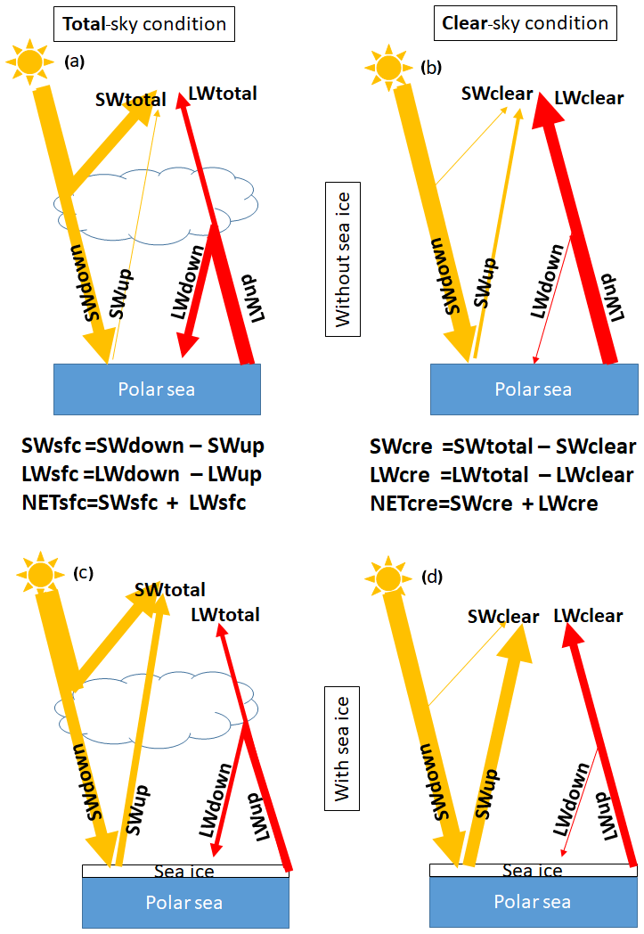
Figure 1 Schematic representation of radiative energy flows in the polar seas under total-sky conditions (a, c) and clear-sky conditions (b, d) for two contrasting surface conditions: without sea ice (a, b) and with sea ice (c, d). All fluxes are taken positive downwards.

2 Methods and data

2.1 CERES EBAF Ed4.0 products

Surface and TOA radiative flux quantities are taken from the NASA CERES Energy Balanced and Filled (EBAF) monthly dataset (CERES EBAF-TOA_Ed4.0 and CERES EBAF-SFC_Ed4.0), providing monthly, global fluxes on a ${\mathrm{1}}^{\circ }\times {\mathrm{1}}^{\circ }$ latitude–longitude grid (Loeb et al., 2018; Kato et al., 2018). CERES surface LW and SW radiative fluxes are used to investigate the effect of clouds on the surface radiation budget response to sea ice variability over the polar seas. CERES SFC EBAF radiative fluxes have been evaluated through comparisons with 46 buoys and 36 land sites across the globe, including the available high-quality sites in the Arctic. Uncertainty estimates for individual surface radiative flux terms in the polar regions range from 12 to 16 W m⁻² (1σ) at the monthly mean ${\mathrm{1}}^{\circ }\times {\mathrm{1}}^{\circ }$ gridded scale (Kato et al., 2018). CERES EBAF-TOA and SFC radiative fluxes show a much higher reliability than other sources (e.g. meteorological reanalysis) and represent a key benchmark for evaluating the Arctic surface radiation budget (Christensen et al., 2016; Loeb et al., 2019; Duncan et al., 2020).

In addition to radiative fluxes, cloud cover fraction (CCF) and cloud optical depth (COD) data available from CERES EBAF data are used. Monthly mean CCF and COD data are derived from instantaneous cloud retrievals using the Moderate Resolution Imaging Spectroradiometer (MODIS) radiances (Trepte et al., 2019). Instantaneous retrievals are then spatially and temporally averaged onto the ${\mathrm{1}}^{\circ }\times {\mathrm{1}}^{\circ }$ monthly-mean grid consistent with CERES EBAF.

2.2 Cloud radiative effect

CRE is used as a metric to assess the radiative impact of clouds on the climate system, defined as the difference in net irradiance at the TOA between total-sky and clear-sky conditions. Using the CERES Energy Balanced and Filled (EBAF) Ed4.0 (Loeb et al., 2018) flux measurements and CMIP5 simulated fluxes, CRE is calculated by taking the difference between clear-sky and total-sky net irradiance flux at the TOA. All fluxes are taken as positive downwards.

$$\begin{array}{}\text{(1)}& {\displaystyle }& {\displaystyle }{\text{SW}}_{\text{cre}}={\text{SW}}_{\text{total}}-{\text{SW}}_{\text{clear }}\text{(2)}& {\displaystyle }& {\displaystyle }{\text{LW}}_{\text{cre}}={\text{LW}}_{\text{total}}-{\text{LW}}_{\text{clear }}\text{(3)}& {\displaystyle }& {\displaystyle }{\text{NET}}_{\text{cre}}={\text{SW}}_{\text{cre}}+{\text{LW}}_{\text{cre }}\end{array}$$

2.3 Earth's surface radiative budget

Surface radiative fluxes are taken from the CERES SFC EBAF Ed4.0 dataset (Kato et al., 2018). The net SW and LW fluxes at the surface (SW_sfc and LW_sfc, respectively) are calculated as the difference between the downwelling SW_down (LW_down) and upwelling SW_up (LW_up) as shown in Eq. (4) (Eq. 5).

$$\begin{array}{}\text{(4)}& {\displaystyle }& {\displaystyle }{\text{SW}}_{\text{sfc}}={\text{SW}}_{\text{down}}-{\text{SW}}_{\text{up }}\text{(5)}& {\displaystyle }& {\displaystyle }{\text{LW}}_{\text{sfc}}={\text{LW}}_{\text{down}}-{\text{LW}}_{\text{up }}\text{(6)}& {\displaystyle }& {\displaystyle }{\text{NET}}_{\text{sfc}}={\text{SW}}_{\text{sfc}}+{\text{LW}}_{\text{sfc }}\end{array}$$

2.4 Sea ice concentration

Sea ice concentration (SIC) data are from the National Snow and Ice Data Center (NSIDC; http://nsidc.org/data/G02202, last access: May 2018). This dataset is a climate data record (CDR) of SIC from passive microwave data and provides a consistent, daily and monthly time series of SIC from 9 July 1987 through the most recent processing for both the northern and southern polar regions (Peng et al., 2013; Meier et al., 2017). The data are provided on a 25 km × 25 km grid. We used the latest version (version 3) of the SIC CDR created with a new version of the input product from Nimbus-7 SMMR (Scanning Multichannel Microwave Radiometer) and DMSP SSM/I-SSMIS Passive Microwave Data (Defense Meteorological Satellite Program Special Sensor Microwave Imager Special Sensor Microwave Imager/Sounder).

2.5 Polar seas

We define the polar seas as ocean regions where the monthly SIC is larger than 10 % for least 1 month during the 2001–2016 period. The extent of the polar seas is shown in Fig. S1.

2.6 CMIP5 models

To reconstruct the historical CRE and surface energy budget and project their future changes, we used an ensemble of simulations conducted with 32 climate models (models used are shown in Figs. 3 and S3) contributing to the Coupled Model Intercomparison Project Phase 5 (CMIP5) (Taylor et al., 2012). These model experiments provided historical runs (1850–2005) in which all external forcings are consistent with observations and future runs (2006–2100) using the RCP8.5 (Representative Concentration Pathway) emission scenarios (Taylor et al., 2012). The comparison with the satellite data is made over 2001–2016 by merging historical runs 2001–2005 with RCP8.5 2006–2016.

2.7 Estimation of the local variations in radiative flux, cloud cover and cloud optical depth concurrent with changes in sea ice concentration

This study employs a novel method for quantifying the variations in radiative fluxes and cloud properties with SIC. This methodology leverages inter-annual variability of sea ice cover to assess these relationships. Figure 2 schematically shows the methodology based on the following steps. We use SW as an example and apply the approach in the same way to other variables.

1. ΔSW_j values are summarised in a schematised plot (Fig. 2a) where each cell j in such plot shows the average ΔSW_m observed for all possible combinations of SIC at a grid box between 2 consecutive observation years (year y_i and y_i+1 from the time period 2001–2016) displayed on the x and y axes, respectively. For the sake of clarity in Fig. 2 the x and y axes report SIC in intervals of 10 %, while in Figs. 5, 6, 7, S5 and S6 the axes are discretised with 2 % bins.

2. Because of the regular latitude–longitude grid used in the analysis, the area of the grid cells (a_m) varies with the latitude. The energy signal (ΔSW_j) is therefore computed as an area-weighted average (Eq. 7), where M is the number of grid cells that are used to compute cell j in the schematised plot of Fig. 2a. Figure 2b shows the total area of all these grid cells as described by Eq. (8).

   $$\begin{array}{}\text{(7)}& {\displaystyle }& {\displaystyle }\mathrm{\Delta }{\text{SW}}_j={\displaystyle \frac{{\sum }_{m=\mathrm{1}}^M{a}_m\mathrm{\Delta }{\text{SW}}_m}{{\sum }_{m=\mathrm{1}}^M{a}_m}}\text{(8)}& {\displaystyle }& {\displaystyle }{A}_j={\sum }_{m=\mathrm{1}}^M{a}_m\end{array}$$

3. Calculation of the area-weighted average (ΔSW_p) of the energy signal of all N cells with the same fraction X of a change in SIC (shown with the same colour in Fig. 2a; Eq. 9).

   $$\begin{array}{}\text{(9)}& \mathrm{\Delta }{\text{SW}}_p={\displaystyle \frac{{\sum }_{j=\mathrm{1}}^N{A}_j\mathrm{\Delta }{\text{SW}}_j}{{\sum }_{j=\mathrm{1}}^N{A}_j}}\end{array}$$

   ${\sum }_{j=\mathrm{1}}^N{A}_j$ is the total area of all grid cells with a particular SIC change. ΔSW_p is the energy-weighted average of all grid cells with a particular SIC change.

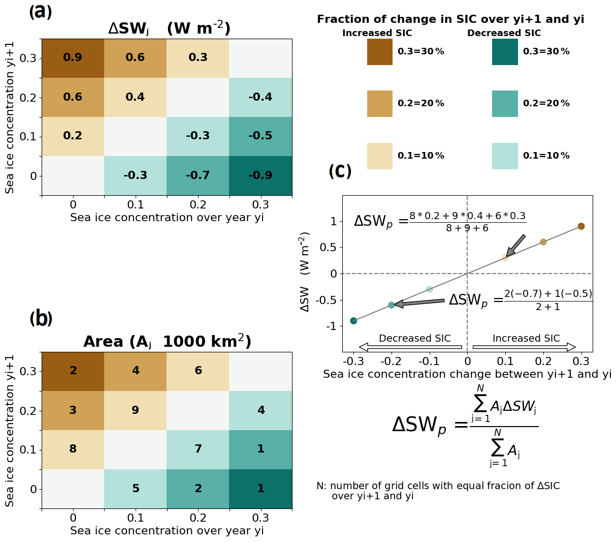
Figure 2 Schematic representation of the methodology used to quantify the energy flux sensitivity to changes in sea ice concentration as a linear regression between the percentage of sea ice concentration and the variation in energy flux (c) using SW energy flux data and sea ice concentration defined in (a, b).

The average energy signals (ΔSW_p) per class of sea ice concentration change are reported in a scatterplot (Fig. 2c) and used to estimate a regression line with zero intercept.

The slope S of this linear regression represents the local SW energy signal generated by the complete sea ice melting of a 1^∘ grid cell. The weighted root mean square error (WRMSE) of the slope is estimated by Eq. (10), where p represents one of the NP points in the scatterplot (NP = 6 in Fig. 2c; number of points) and X_p is the relative change in sea ice concentration in the range ±1 (equivalent to ±100 % of sea ice cover change).

$$\begin{array}{}\text{(10)}& \text{WRMSE}=\sqrt{{\displaystyle \frac{{\sum }_{p=\mathrm{1}}^{\text{NP}}{A}_p{\left(\mathrm{\Delta }{\text{SW}}_p-S{X}_p\right)}^{\mathrm{2}}}{{\sum }_{p=\mathrm{1}}^{\text{NP}}{A}_p}}},\end{array}$$

where $A_p={\sum }_{j=\mathrm{1}}^N{A}_j$.

2.8 Diagnosis of contributions to SW_cre

SW_cre at the surface for the year y_i (Eq. 11) and year y_i+1 (Eq. 12) is function of surface albedo α, SW_down under clear-sky conditions (SW↓_clr) and SW_down under total-sky conditions (SW↓_tot).

$$\begin{array}{}\text{(11)}& {\displaystyle }& {\displaystyle }{\text{SWcre}}_{y_i}=\left(\mathrm{1}-{\mathit{\alpha }}_{y_i}\right)(\text{SW}{\downarrow }_{\text{tot},y_i}-\text{SW}{\downarrow }_{\text{clr},y_i})\text{(12)}& {\displaystyle }& {\displaystyle }{\text{SWcre}}_{y_{i+\mathrm{1}}}=\left(\mathrm{1}-{\mathit{\alpha }}_{y_{i+\mathrm{1}}}\right)(\text{SW}{\downarrow }_{\text{tot},y_{i+\mathrm{1}}}-\text{SW}{\downarrow }_{\text{clr},y_{i+\mathrm{1}}})\end{array}$$

Using the first-order Taylor series expansion to Eq. (11) yields

$$\begin{array}{}\text{(13)}& \begin{array}{rl}\mathrm{\Delta }{\text{SWcre}}_{y_{i+\mathrm{1}}-y_i}& \cong \left(-\mathrm{\Delta }{\mathit{\alpha }}_{y_{i+\mathrm{1}}-y_i}\right)\left(\text{SW}{\downarrow }_{\text{tot},y_i}-\text{SW}{\downarrow }_{\text{clr},y_i}\right)\\ & +\left(\mathrm{1}-{\mathit{\alpha }}_{y_i}\right){\mathrm{\Delta }}_{y_{i+\mathrm{1}}-y_i}(\text{SW}{\downarrow }_{\text{tot}}-\text{SW}{\downarrow }_{\text{clr}}),\end{array}\end{array}$$

where

$$\begin{array}{}\text{(14)}& \begin{array}{rl}{\mathrm{\Delta }}_{y_{i+\mathrm{1}}-y_i}\left(\text{SW}{\downarrow }_{\text{tot}}-\text{SW}{\downarrow }_{\text{clr}}\right)& \cong \left(\text{SW}{\downarrow }_{\text{tot},y_{i+\mathrm{1}}}-\text{SW}{\downarrow }_{\text{clr},y_{i+\mathrm{1}}}\right)\\ & -(\text{SW}{\downarrow }_{\text{tot},y_i}-\text{SW}{\downarrow }_{\text{clr},y_i}).\end{array}\end{array}$$

Separating the terms yields

$$\begin{array}{}\text{(15)}& \mathrm{\Delta }{\text{SW}}_{\text{cre}}\text{Alb}\cong \left(-\mathrm{\Delta }{\mathit{\alpha }}_{y_{i+\mathrm{1}}-y_i}\right)(\text{SW}{\downarrow }_{\text{tot},y_i}-\text{SW}{\downarrow }_{\text{clr},y_i}),\end{array}$$

where ΔSW_creAlb is the part of SW_cre change that is induced by the change in surface albedo, and

$$\begin{array}{}\text{(16)}& \mathrm{\Delta }{\text{SW}}_{\text{cre}}\text{Cloud}\cong \left(\mathrm{1}-{\mathit{\alpha }}_{y_i}\right){\mathrm{\Delta }}_{y_{i+\mathrm{1}}-y_i}(\text{SW}{\downarrow }_{\text{tot}}-\text{SW}{\downarrow }_{\text{clr}}),\end{array}$$

where ΔSW_creCloud is the part of SW_cre change that is induced by the change in cloud cover and cloud optical depth.

$$\begin{array}{}\text{(17)}& \mathrm{\Delta }{\text{SWcre}}_{y_{i+\mathrm{1}}-y_i}\cong \mathrm{\Delta }{\text{SW}}_{\text{cre}}\text{Alb}+\mathrm{\Delta }{\text{SW}}_{\text{cre}}\text{Cloud}\end{array}$$

The above equations are used in Figs. 7 and S5.

3 Results and discussions

3.1 Negative correlation patterns between cloud radiative effect and surface radiation on polar seas

Given the known cloud influence on the surface radiative budget, a positive correlation between TOA CRE and surface radiative budget is expected (the amount of absorbed radiation at the surface decreases with a more negative SW_cre and a less positive LW_cre). Figure 3 illustrates a positive correlation between the annual-mean NET_cre and NET_sfc over much of the global ocean using the CERES TOA flux data from 2001 to 2016. However, our analysis reveals the opposite pattern over the polar seas (defined in Sect. 2.5) where the correlation is negative over the Antarctic and partly negative over the Arctic (Bering Strait, Hudson Bay, Barents Sea and the Canadian Archipelago; Fig. 3a, b). Considering the SW_cre and LW_cre components, we find that the SW_cre (Fig. 3c, d) shows a similar pattern of correlation as the NET_cre (Fig. 3a, b) but with a stronger magnitude, while LW_cre generally shows the opposite correlations (Fig. 3e, f). This suggests that the factors influencing SW_cre are responsible for the sharp contrast in the correlation found in the polar regions. Indeed, SW_sfc and SW_cre (Fig. 3g, h) show the sharpest and most significant contrast between the polar regions and the rest of the world (Fig. S2 is similar to Fig. 3, but only significant correlations at the 95 % confidence level are reported in blue and red colours). Overall, climate models are able to reproduce the spatial pattern of the observed SW correlation but also show a large inter-model spread in the spatial extent of the phenomena (Figs. 4 and S3). On the other hand, several models completely fail to reproduce the correlation. The ACCESS1-3, MIROC5, CanESM2 and CSIRO-Mk3-6-0 models show a negative correlation over the Antarctic continent in contrast to an observed positive correlation. Some models, like IPSL-CM5B-LR, GISS-E2-R and bcc-csm1-1, fail to reproduce the observed negative correlation over the Antarctic Ocean. This suggests that these models contain misrepresentations of the relationships of SW_cre and NET_sfc, likely resulting from errors in the relationships between sea ice, surface albedo, cloud cover and thickness, and their influence on surface radiative fluxes that could severely impact their projections. Moreover, Fig. 4 demonstrates that simple correlations between NET_sfc and the individual radiation budget terms represent a powerful metric for climate model evaluation that allows for a quick check for realistic surface radiation budget variability in polar regions.

Figure 3 Correlation between TOA CRE and surface radiation budget terms over 2001–2016 from CERES measurements for the Northern Hemisphere (a, c, e, g) and Southern Hemisphere (b, d, f, h) polar sea. Positive correlations shown by the red colours indicate that years with less NET_sfc coincide with years where NET_cre has a stronger cooling effect and vice versa.

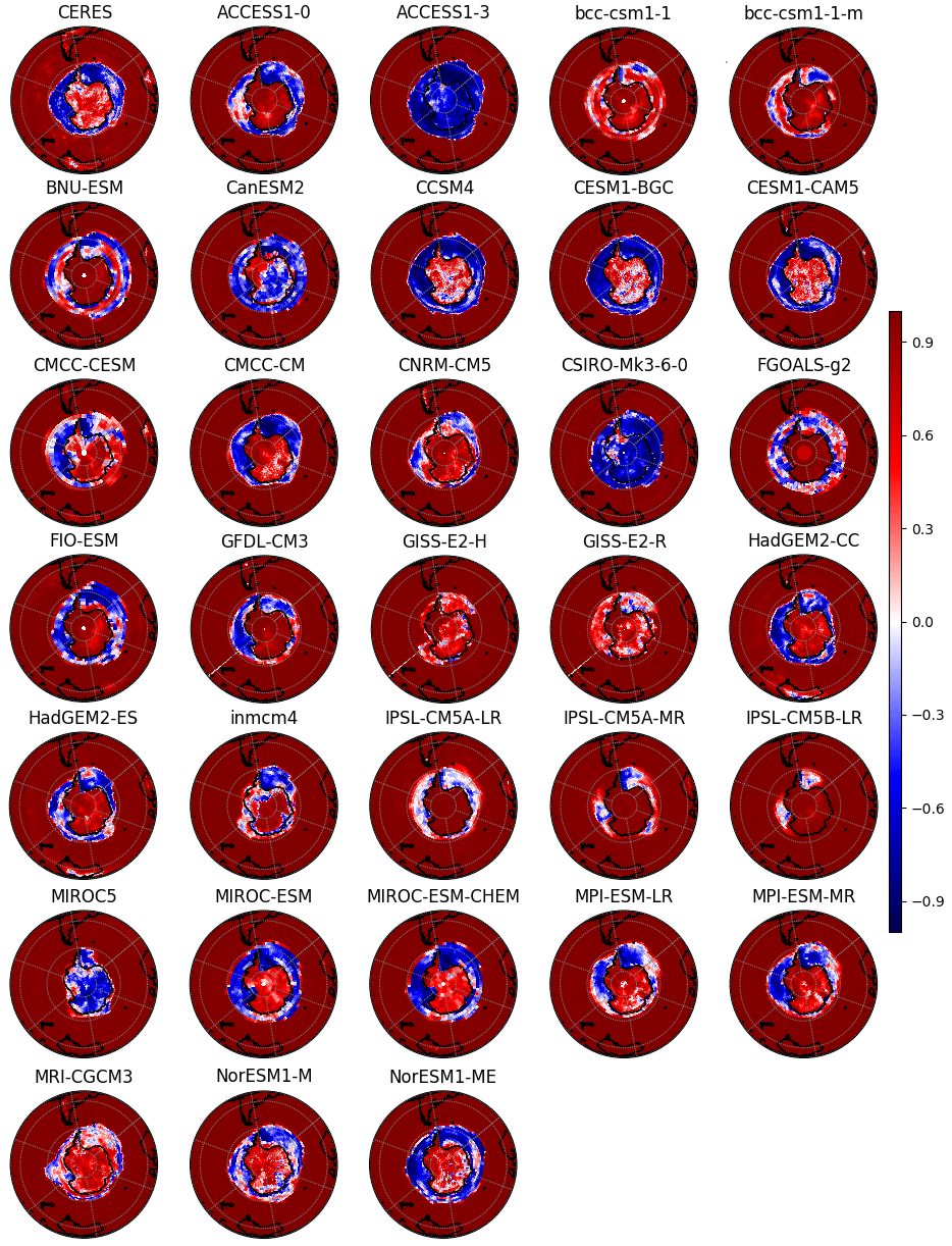
Figure 4 Correlation between SW_cre and SW_sfc shown by 32 CMIP5 Earth system models and CERES between 2001 and 2016 over the Southern Hemisphere.

3.2 Effects of sea ice concentration change

We illustrate that the apparent contradiction over the polar seas between NET_cre and NET_sfc found in Fig. 3a, b is caused by the factors contributing to the SW fluxes. This can be explained by the following. (i) SW_cre can change even if cloud properties are held constant due to the changes in clear-sky radiation induced by changes in sea ice and surface albedo. When surface albedo is reduced, the surface absorbs more sunlight at the surface, resulting in a greater SW_total. At the same time, SW_clear increases, since the lower albedo allows a larger fraction of the extra downwelling SW at the surface to be absorbed (see Fig. 1). Therefore, SW_cre becomes more negative even in the absence of cloud changes (a purely surface-related effect). (ii) On the other hand, the relationship between cloud cover and thickness and sea ice could lead to cloudier polar seas under melting sea ice (Abe et al., 2016; Liu et al., 2012) such that the SW_cre decreases (increasing the amount of SW reflected back to space by clouds; see Fig. 1); thus the cloud cooling effect is enhanced concurrently with melting sea ice (a purely cloud-related effect). Both of these factors occur simultaneously.

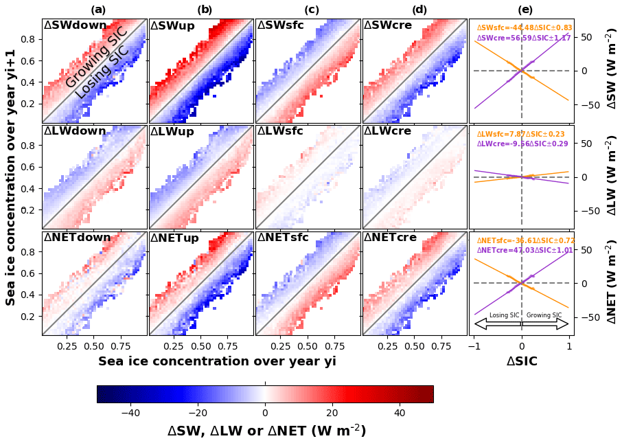
Figure 5 Annual changes in SW, LW and NET as a function of SIC. Annual changes in SW (top), LW (middle) and NET (bottom) of radiative down (a), up (b), sfc = down-up (c) and cre (d) over the Antarctic Ocean as a function of SIC change between 2 consecutive years, y_i+1 and y_i, from the 2001 to 2016 time period. The top triangles in (c top) refer to the increase (growing) in SIC, while the blue colours mean a reduction (cooling) in SW_sfc. The top triangles in (d) refer to the increase in SIC, while the red colours mean an increase (decreasing the cooling role of clouds) in SW_cre. Each dot in column (e) represents the average of one parallel to the diagonal in (c) or (d) as described in Sect. 2.7.

Over the Antarctic Ocean, analysis of the year-to-year changes in SW_down stratified in 2 % SIC bins retrieved from satellite microwave radiometer measurements (see Sect. 2.7) shows an increase in SW_down with increased SIC and vice versa (Fig. 5a). This suggests that years with higher SIC also have fewer and/or thinner clouds (Liu et al., 2012) (Fig. 6), larger SW_down and also larger upward SW radiation (SW_up) (Fig. 5b), due to higher surface albedo (Fig. S4). Consequently, these years show a more negative SW_sfc (Fig. 5c) and thus are characterised by stronger surface cooling. Furthermore, the presence of fewer clouds implies a reduction of the cloud cooling effect (less negative SW_cre) as described above in process (ii); this accounts for $(\mathrm{19.42}\times \mathrm{100})/\mathrm{56.59}=\mathrm{34}\pm \mathrm{1}$ % (Fig. 7d bottom) of the total change in SW_cre, and as described in process (i) the increase in the surface albedo also makes SW_cre less negative and explains $(\mathrm{37.17}\times \mathrm{100})/\mathrm{56.59}=\mathrm{66}\pm \mathrm{2}$ % of the observed change (Fig. 7d bottom). Thus, the observed negative correlation between SW_cre and SW_sfc over the polar seas results from the larger effects of process (i) than (ii). Similar results are found over the Arctic Ocean with a slightly different sensitivity (Figs. S5, S6). This difference is tied to differences in sun angle and available sunlight, as Antarctic sea ice is concentrated at lower latitudes than Arctic sea ice.

Using the regression relationships derived from our composite analysis, we estimate the magnitude of the cloud effect. For the Antarctic system, we use the numbers found in Fig. 5e where we find the annual-mean relationship between NET_sfc (in W m⁻²) and SIC (fraction between 0 and 1) and NET_cre (in W m⁻²) and SIC (fraction between 0 and 1).

$$\begin{array}{}\text{(18)}& {\displaystyle }& {\displaystyle }\mathrm{\Delta }{\text{NET}}_{\text{sfc}}=(-\mathrm{36.61}\pm \mathrm{0.72})\mathrm{\Delta }\text{SIC}\text{(19)}& {\displaystyle }& {\displaystyle }\mathrm{\Delta }{\text{NET}}_{\text{cre}}=(\mathrm{47.03}\pm \mathrm{1.01})\mathrm{\Delta }\text{SIC}\end{array}$$

When excluding the CRE, the ΔNET_sfc would be equal to (−36.61–47.03) $\mathrm{\Delta }\text{SIC}=-\mathrm{83.64}\mathrm{\Delta }\text{SIC}$.

We estimate that the existence of clouds and their property variations are damping the potential increase in the NET_sfc within the Antarctic system due to the surface albedo decrease from sea ice melt by 56 % (47.03/83.64). The uncertainty is calculated by summing the uncertainties shown in Eqs. (18) and (19) as follows: $({\mathrm{0.72}}^{\mathrm{2}}+{\mathrm{1.01}}^{\mathrm{2}}{)}^{\mathrm{1}/\mathrm{2}}/\mathrm{83.64}=\mathrm{2}$ %.

Similarly, over the Arctic (Fig. S5), we compute the cloud influence on the surface net radiative budget that covaries with sea ice loss is 47±3 %, in agreement with the study of Sledd and L'Ecuyer (2019).

Figure 6 Seasonal and annual changes in cloud cover fraction (CCF) and cloud optical depth (COD) over the Antarctic polar sea region as a function of SIC change between 2 consecutive years, y_i+1 and y_i, from the 2001 to 2016 time period. In order to use the same scale, COD has been multiplied by a factor of 10. The top triangles in the two first columns refer to the increase (growing) in SIC, while the blue colours mean a reduction in CCF or COD.

Figure 7 Seasonal and annual changes in SW_creAlb, SW_creCloud and SW_cre over the Antarctic polar sea region as a function of SIC change between 2 consecutive years, y_i+1 and y_i, from the 2001 to 2016 time period. The analysis is based on the method described in Sect. 2.7 and observations from satellites data.

Altogether the results suggest that clouds substantially reduce the impact of sea ice loss on the surface radiation budget and thus the observed sea ice albedo feedback. This effect in the polar climate system leads to a substantial reduction (56±2 % over the Antarctic and 47±3 % over the Arctic) of the potential increase in NET_sfc in response to sea ice loss. This magnitude is similar to a previous study (Qu and Hall, 2006) showing that across a climate model ensemble clouds damped the TOA effect of land surface albedo variations by half. Sledd and L'Ecuyer (2019) also determined that the cloud damping effect (also referred to as cloud masking) of the TOA albedo variability results from Arctic sea ice changes was approximately half. Despite this mechanism, the sharp reduction in Arctic surface albedo has dominated the recent change in the surface radiative budget and has led to a significant increase in NET_sfc since 2001 in the CERES data (Duncan et al., 2020). These results demonstrate that the trends in polar surface radiative fluxes are driven by reductions in SIC and surface albedo and that clouds have partly mitigated the trend (i.e. a damping effect). Our findings highlight the importance of processes that control sea ice albedo (i.e. sea ice dynamics, snowfall, melt pond formation and the deposition of black carbon), as the surface albedo of the polar seas in regions of seasonal sea ice is crucial for the climate dynamics.

3.3 Sensitivity of the surface energy budget to variability of sea ice concentration

Our results are consistent with other recent studies (Taylor et al., 2015; Morrison et al., 2018) that demonstrate a CCF response to reduced sea ice in autumn and winter but not in summer (Fig. 8a) over the Arctic Ocean. The lack of a summer cloud response to sea ice loss is explained by the prevailing air–sea temperature gradient, where near-surface air temperatures are frequently warmer than the surface temperature (Kay and Gettelman, 2009). Surface temperatures in regions of sea ice melt hover near freezing due to the phase change, whereas the atmospheric temperatures are not constrained by the freezing–melting point. Despite reduced sea ice cover, increases in surface evaporation (latent heat) are limited (Fig. 8m, n), as also suggested by the small trends in the surface evaporation rate derived from satellite-based estimates (Boisvert and Stroeve, 2015; Taylor et al., 2018). We argue that the strong increase of SW_creCloud under decreased sea ice observed during summer is induced by larger values of COD (Fig. 8a), which depend on the liquid or ice water content. We also show that the relationships derived from our observation-driven analysis match the projected changes in the Arctic and Antarctic surface energy budget in the median CMIP5 model ensemble (Fig. 8). However, we find a large spread amongst climate models that indicates considerable uncertainty.

Analysing the seasonal cycle of the sensitivity of the surface energy budget to SIC variability, we found that SW_sfc (SW_cre) explains most of the observed changes in the NET_sfc (NET_cre) during summer, while LW_sfc plays a minor role (Fig. 8). In contrast, during winter LW_sfc (LW_cre) explains most of the observed changes in the NET_sfc (NET_cre). In general, the median of the 32 CMIP5 (Taylor et al., 2012) climate models captures the observed sensitivity of the radiative energy budget and cloud cover change to SIC, but the spread between climate models is large, especially for CCF. We have to note here that the numbers reported in Fig. 8 are for 100 % SIC loss, while the ones reported in the previous figures (Figs. 5, 6 and 7) are for 100 % SIC gain, explaining the opposite sign.

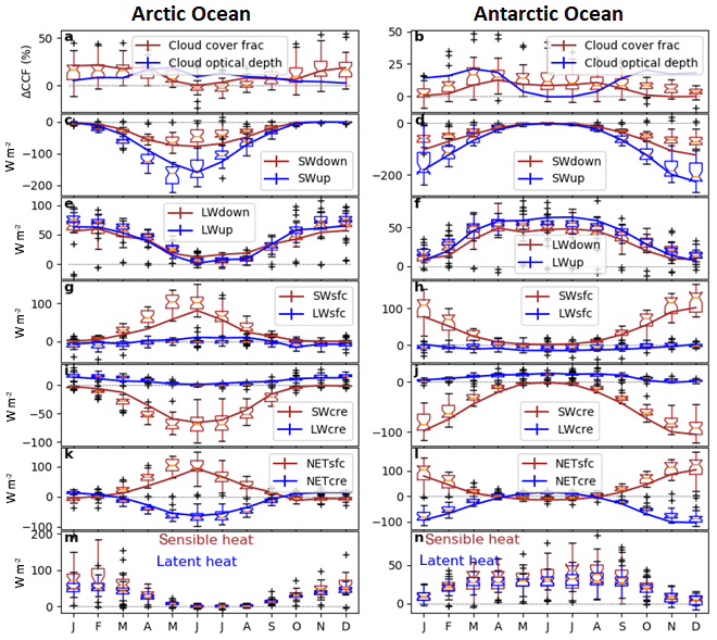
Figure 8 Monthly change in different terms of the radiative energy balance, cloud optical depth (COD) and cloud cover fraction (CCF) extrapolated from observations for a hypothetical 100 % decrease in SIC over the areas where SIC change was observed during the period 2001–2016. This estimate came from the use of a linear interpolation of the change of different parts of the energy budget, COD and CCF as a function of a change in SIC coming from all possible combinations of couplets of consecutive years for a given month from 2001 to 2016, and for all grid cells for which SIC is larger than zero in 1 of the 2 years (see Sect. 2.7). CERES data are shown by solid lines (the standard deviation of the slopes are also reported but are too small to be visible), while CMIP5 models are shown by boxplot, and the box (in the same colour as observations) represents the first and third quartiles (whiskers indicate the 99 % confidence interval, and black markers show outliers). In order to use the same scale, COD has been multiplied by a factor 10.

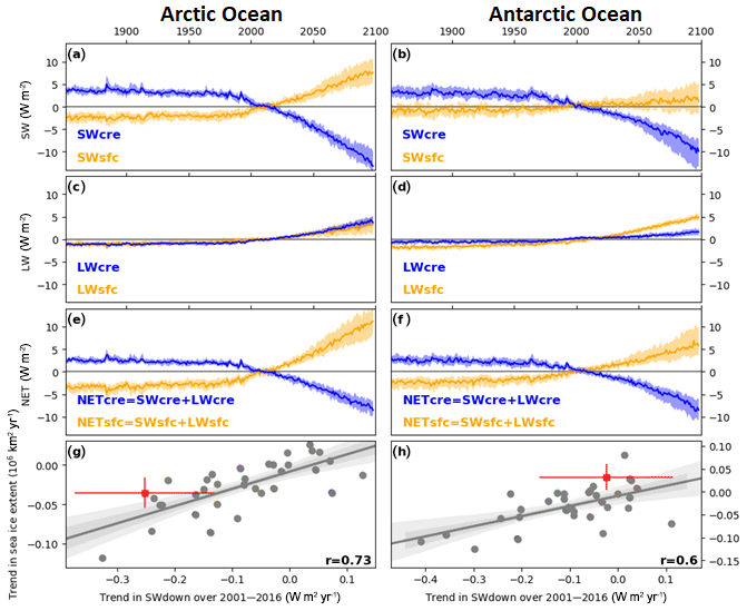
Figure 9 Time series of the anomaly with respect to the whole period 1850–2100 of the radiative flux. Mean modelled SW_cre, LW_cre and NET_cre (blue) and surface SW_sfc, LW_sfc and NET_sfc (orange) anomalies over the 1850–2100 period under the RCP8.5 scenario averaged over the Arctic Ocean. The solid line shows the median, where the envelope represents the 25th and 75th percentile of the 32 CMIP5 models. The linear regression (grey solid line and its 68 % – dark-grey envelope – and 95 % – light-grey envelope – confidence interval) between the trend in SW_down and trend in sea ice extent (g, h) of the 32 CMIP5 climate models shown by grey dots over 2001–2016. The observed trends are shown by red colours, where the confidence interval refers to the standard error of the trend.

3.4 Projections and uncertainties of cloud radiative effects on the surface energy budget

Under the RCP8.5 scenario (“business as usual”; Taylor et al., 2012), CMIP5 models show an increase in SW_sfc over the Arctic Ocean (Fig. 9a), consistent with the expected decrease in the SIC (Comiso et al., 2008; Serreze et al., 2007; Stroeve et al., 2007). This increase in SW_sfc occurs despite the large, concurrent and opposing change in SW_cre. Projections of LW flux changes (Fig. 9c) are expected to play a small but non-negligible role on the total energy budget in summer by slightly increasing NET_sfc (Fig. 9e). In addition, CMIP5 models indicate that by 2100 the magnitude of the NET_cre decrease will be slightly smaller than the increase in NET_sfc (Fig. 9e) over the Arctic Ocean, while the Antarctic polar sea region shows the opposite (Fig. 9f). This is in line with the estimated damping effect of clouds coming from CERES over 2001–2016 that is about 47±3 % in the Arctic and 56±2 % in the Antarctic. The stronger cloud damping effect in the Antarctic region is indicated by the stronger negative change in NET_cre in the Antarctic compared to the Arctic (Fig. 9e, f).

Large uncertainties remain in the rate of summer sea ice decline and the timing of the first sea-ice-free Arctic summer (Arzel et al., 2006; Zhang and Walsh, 2006). The processes responsible for the large inter-model spread between climate models are still under scrutiny (Holland et al., 2017; Simmonds, 2015; Turner et al., 2013). However, recent studies reaffirm the important role of the sea ice albedo feedback and the associated increased upper Arctic Ocean heat content (Holland and Lundrum, 2015; Boeke and Taylor, 2018) as well as the contributions from temperature-related feedbacks (Pithan and Maruitsen, 2014; Stuecker et al., 2018). Figure 9g, h shows that the annual-mean Arctic and Antarctic sea ice extent trend from 32 CMIP5 models possesses a large positive correlation with the simulated trend in the SW_down, in line with previous studies (Holland and Lundrum, 2015). We note that from the 32 CMIP5 models tested, only a few show SW_down trends consistent with observed trends in SW_down and SIC over 2001–2016 (Fig. 9g, h). Understanding the factors responsible for this disagreement between model-simulated and observed trends in SW_down and SIC may provide insights into the processes responsible for the inter-model spread in Arctic climate change projections and are the subject of future work. We also find that the models with a larger trend in cloud cover also possess a larger decrease in sea ice extent, suggesting a stronger coupling between these two variables that may become stronger in the future. However, the direction of causality between the two variables is unclear and also requires further study.

4 Conclusion

The paper addresses two important climate science topics, namely the role of clouds and the fate of polar sea ice. The work is grounded in a long time series of robust satellite observations that allowed us to document an important damping effect in the polar cloud–sea-ice system using a unique inter-annual approach. Our results agree with several previous works that approached the problem from a different perspective (Hartmann and Ceppi, 2014; Sledd and L'Ecuyer, 2019). In addition, we show how 32 state-of-the-art climate models represent aspects of the surface radiation budget over the polar seas.

Our data-driven analysis shows that polar sea ice and clouds interplay in a way that substantially reduces the impact of the sea ice loss on the surface radiation budget. We found that when sea ice cover is reduced between 2 consecutive years, the cloud radiative effect becomes more negative, damping the total change in the net surface energy budget. The magnitude of this effect is important. Satellite data indicate that the more negative cloud radiative effect reduces the potential increase of net radiation at the surface by approximately half. One-third of this cloud radiative effect change is induced by the direct change in cloud cover and thickness, while two-thirds of this change results from the surface albedo change.

In addition, we demonstrated that the models that show larger trends in polar sea ice extent also show larger trends in surface incoming solar radiation. In order to understand current and future climate trajectories, model developments should aim at reducing uncertainties in the representation of polar cloud processes in order to improve the simulation of present-day cloud properties over the polar seas. Present-day Arctic and Antarctic cloud properties strongly influence the model-simulated cloud damping effect on the radiative impacts of sea ice loss.

Future cloud changes and sea ice evolution represent major uncertainties in climate projections due to the multiple relevant pathways through which cloudiness and sea ice feed back on Earth's climate system (Solomon et al., 2007). Our evidence derived from Earth observations provides additional insight into the coupled radiative impacts of polar clouds and the changing sea ice cover (Fig. 8) that may provide a useful constraint on model projections and ultimately improve our understanding of present and future polar climate. On a practical level, our results demonstrate a simple correlation analysis between the net surface radiation budget and individual radiation budget terms that can be used to quickly evaluate climate models for realistic surface radiation budget variability in polar regions. Ultimately, our findings on the interplay between clouds and sea ice may support an improvement in the model representation of the cloud–ice interactions, mechanisms that may substantially affect the speed of the polar sea ice retreat, which in turn has a broad impact on the climate system, on the Arctic environment and on potential economic activities in the Arctic region (Buixadé Farré et al., 2014).