Satellite passive microwave sea-ice concentration data set inter-comparison for Arctic summer conditions

We report on results of a systematic inter-comparison of 10 global sea-ice concentration (SIC) data products at 12.5 to 50.0 km grid resolution from satellite passive microwave (PMW) observations for the Arctic during summer. The products are compared against SIC and net ice surface fraction (ISF) – SIC minus the per-grid-cell melt pond fraction (MPF) on sea ice – as derived from MODerate resolution Imaging Spectroradiometer (MODIS) satellite observations and observed from ice-going vessels. Like in Kern et al. (2019), we group the 10 products based on the concept of the SIC retrieval used. Group I consists of products of the European Organisation for the Exploitation of Meteorological Satellites (EUMETSAT) Ocean and Sea Ice Satellite Application Facility (OSI SAF) and European Space Agency (ESA) Climate Change Initiative (CCI) algorithms. Group II consists of products derived with the Comiso bootstrap algorithm and the National Oceanographic and Atmospheric Administration (NOAA) National Snow and Ice Data Center (NSIDC) SIC climate data record (CDR). Group III consists of Arctic Radiation and Turbulence Interaction Study (ARTIST) Sea Ice (ASI) and National Aeronautics and Space Administration (NASA) Team (NT) algorithm products, and group IV consists of products of the enhanced NASA Team algorithm (NT2). We find widespread positive and negative differences between PMW and MODIS SIC with magnitudes frequently reaching up to 20 %–25 % for groups I and III and up to 30 %–35 % for groups II and IV. On a pan-Arctic scale these differences may cancel out: Arctic average SIC from group I products agrees with MODIS within 2 %–5 % accuracy during the entire melt period from May through September. Group II and IV products overestimate MODIS Arctic average SIC by 5 %–10 %. Out of group III, ASI is similar to group I products while NT SIC underestimates MODIS Arctic average SIC by 5 %–10 %. These differences, when translated into the impact computing Arctic sea-ice area (SIA), match well with the differences in SIA between the four groups reported for the summer months by Kern et al. (2019). MODIS ISF is systematically overestimated by all products; NT provides the smallest overestimations (up to 25 %) and group II and IV products the largest overestimations (up to 45 %). The spatial distribution of the observed overestimation of MODIS ISF agrees reasonably well with the spatial distribution of the MODIS MPF and we find a robust linear relationship between PMW SIC and MODIS ISF for group I and III products during peak melt, i.e. July and August. We discuss different cases taking into account the expected influence of ice surface properties other than melt ponds, i.e. wet snow and coarse-grained snow/refrozen surface, on brightness temperatures and their ratios used as input to the SIC retrieval algorithms. Based on this discussion we identify the mismatch between the actually observed surface properties and those represented by the ice tie points as the most likely reason for (i) the observed differences between PMW SIC and MODIS ISF and for (ii) the often surprisingly small difference between PMW and MODIS SIC in areas of high melt pond fraction. We conclude that all 10 SIC products are highly inaccurate during summer melt. We hypothesize that the unknown number of melt pond signatures likely included in the ice tie points plays an important role – particularly for groups I and II – and recommend conducting further research in this field.

1 Introduction

A considerable number of different algorithms to compute the sea-ice concentration from satellite passive microwave (PMW) brightness temperature (TB) measurements have been developed during the past decades. All exploit the fact that under typical viewing angles (50–55^∘) the difference in microwave TB between open water and sea ice is sufficiently large to estimate sea-ice concentration.

In the polar regions, freezing conditions prevail during winter. During summer, melting conditions prevail or at least coexist with freezing conditions. The changes in snow and sea-ice properties in response to the melting conditions complicate the retrieval of the sea-ice concentration from microwave TB measurements. This applies in particular to the Arctic. The first signs of melt are an increase in snow wetness and melt–refreeze cycles, triggered by diurnal warming and nocturnal cooling, leading to an increase in snow grain size and snow density. Wet snow is a good absorber of microwave radiation and has an emissivity close to 1. Therefore, microwave TBs measured over wet snow are often very close to the physical temperature of the melting snow, i.e. 0 ^∘C. As a consequence, wet snow masks the radiometric difference between different ice types, e.g. first-year and multi-year ice. Above a certain wetness and snow thickness (a few centimetres), the influence of wet snow on microwave TBs in the frequency range used here (see Table 1) can be regarded as being independent of frequency and polarization. The influence of coarse-grained snow is more complex. During diurnal melting, it behaves like wet snow. During nocturnal cooling, the liquid water refreezes and absorbs considerably less microwave radiation. This allows for volume scattering from within the snow, which – in contrast to the absorption of microwave radiation by wet (coarse-grained) snow – is both frequency and polarization dependent. More details about the influence of these parameters on microwave TBs relevant for retrieval of sea-ice concentration during summer are given, e.g., in Kern et al. (2016).

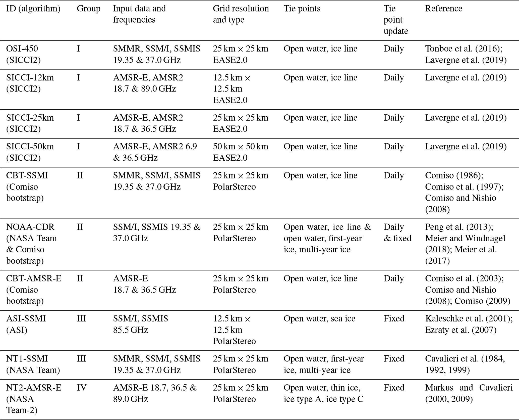
Table 1 Overview of the investigated sea-ice concentration products. Column “ID (algorithm)” holds the identifier we use henceforth to refer to the data product and which algorithm it uses. Group is an identifier for the algorithm concept used. Column “Input data” refers to the input satellite data for the data set. Columns “Tie points” and “Tie point update” refer to the type of tie points used and their update interval (see text for further details).

Continued melting results in increasing snow wetness until it becomes saturated with meltwater – at which stage melt ponds start to form. The fraction of the ice surface covered by melt ponds formed from melting snow and sea ice typically varies between 10 % and 40 % but it can exceed 50 %, e.g., early in the melt season and on particularly level sea ice such as land-fast sea ice (e.g. Webster et al., 2015; Divine et al., 2015; Landy et al., 2014). The fraction of liquid water due to melt ponds on the sea ice poses a particular challenge for the sea-ice concentration retrieval using microwave TB measurements because the penetration depth of microwaves in water at the frequencies listed in Table 1 is of the order of 1 mm (Ulaby et al., 1986). Thus, a water layer with a depth of only a few millimetres is sufficiently opaque to block the thermal microwave emission of the sea ice underneath completely. In addition, the emissivity of fresh water in the ponds and the emissivity of saline water in the leads are the same at most of the microwave frequencies above 10 GHz that we use here. Therefore, during summer liquid water in the form of melt ponds on the sea ice is indistinguishable from liquid water in the cracks and leads between the ice floes in the microwave frequency range used here (e.g. Gogineni et al., 1992; Grenfell and Lohanick, 1985). This has direct consequences for the sea-ice concentration retrieval using satellite TB measurements.

Several studies have revealed various degrees of underestimation of the sea-ice concentration during summer conditions in the Arctic (e.g. Ivanova et al., 2015; Rösel et al., 2012b; Markus and Dokken, 2002; Comiso and Kwok, 1996; Steffen and Schweiger, 1991; Cavalieri et al., 1990). A natural explanation of this observed underestimation would therefore be that those satellite products are rather a good measure of the “net ice surface fraction”, that is 1 minus the area fraction of all surface water in the satellite field of view. We illustrate the typical summer sea-ice concentration retrieval by a simple example. Consider two grid cells A and B observed during the summer melt season. Grid cell A has 100 % sea-ice cover with 40 % melt pond fraction. Grid cell B has 75 % sea-ice cover with 15 % melt ponds. Based on physical principles a sea-ice concentration retrieval algorithm should provide a value of 60 % in both cases, i.e. the so-called “net ice surface fraction”. There is evidence from literature (e.g., Comiso and Kwok, 1996; Kern et al., 2016) that this is however not the case. It is rather very likely that an algorithm would provide a value of, for instance, 85 % for both grid cells A and B, because melt-induced changes in the surface emissivity of the visible part of the sea ice are often insufficiently taken into account, yielding an overestimation of the actual net ice surface fraction. Providing a value of 85 %, this algorithm would underestimate the actual sea-ice concentration in grid cell A by 15 % while it would overestimate it by 10 % in grid cell B. If we interpret the provided value as a net ice surface fraction, it is an overestimation by 25 % in both cases. In other words, for this quite typical example the retrieved value is highly inaccurate and biased compared to either the actual sea-ice concentration or the net ice surface fraction. The magnitude of this bias is largely unknown and it appears not to be reflected by an appropriate increase in retrieval uncertainty estimates which – when at all provided – are a measure of the precision, i.e. the interval within which the reported sea-ice concentration estimate typically varies, and not of the bias. In Fig. 1 we show the seasonal cycle of the sea-ice concentration algorithm standard error – the precision – of the OSI-450, SICCI-25km, and SICCI-50km products (Lavergne et al., 2019) for illustration; OSI-450 and SICCI are product names for SIC climate data records (CDRs) derived from a collaboration of European Organisation for the Exploitation of Meteorological Satellites (EUMETSAT) Ocean and Sea Ice Satellite Application Facility (OSI SAF) and European Space Agency (ESA) Climate Change Initiative (CCI) programmes (see Lavergne et al., 2019). To summarize, we do not know what the sea-ice concentration algorithms actually measure during summer (actual sea-ice concentration or net sea-ice surface fraction), and whichever they measure the accuracy is poor compared to the winter conditions.

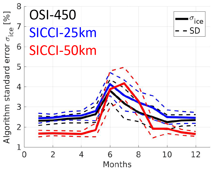
Figure 1 Seasonal cycle of the multi-annual (2002–2011) average sea-ice concentration algorithm standard error for the Arctic for grid cells with more than 90 % sea-ice concentration for OSI-450, SICCI-25km, and SICCI-50km products. Shown are the mean (solid line) and its standard deviation (dashed line denoted “SD”).

The unknown accuracy makes it difficult if not impossible to use summer satellite PMW sea-ice concentration maps and sea-ice area (SIA) for the evaluation of numerical models (e.g., Notz, 2014; Burgard et al., 2020), or to assimilate such data into numerical models for a quantitative improvement of, e.g., sea-ice forecast for shipping (e.g., Melia et al., 2017). As a consequence, studies about the long-term development of the Arctic sea-ice cover prefer to use sea-ice extent (SIE) over SIA. The SIE is computed as the sum of all grid cells with more than 15 % sea-ice concentration: $\text{SIE}=\sum A_{\text{SIC}>\mathrm{15}\mathit{\%}}$, with grid-cell area A. The SIA includes the actual SIC as weight $\text{SIA}=\sum \left(A\times \frac{\text{SIC}}{\mathrm{100}\mathit{\%}}\right)$; a SIC threshold of 15 % is not applied regularly. Consequently, biases in the sea-ice concentration certainly have a small influence on the summer SIE while the impact on SIA can be quite large (see for example Kern et al., 2019, Figs. 6, G2 and G3). However, it has been found that the SIE and its trend provide a limited metric for the performance of numerical models (e.g., Notz, 2014) and that prediction of the minima in September Arctic SIA and SIE would benefit from giving more weight to SIA (e.g. Petty et al., 2018). One way to overcome the SIA biases in summer could be to focus on its trends (as opposed to its absolute value) (e.g. Comiso et al., 2017; Ivanova et al., 2014), but this cannot be the solution since there is no guarantee that these biases are stable along the whole time series.

With this study, we aim to give more information about the accuracy of current satellite PMW sea-ice concentration products during summer. We present a systematic inter-comparison of 10 such products (see Sect. 2 and Kern et al., 2019) with independent estimates of the summertime Arctic sea-ice concentration, net ice surface fraction, and melt pond fraction derived from observations of the MODerate resolution Imaging Spectroradiometer (MODIS) aboard the Earth Observation Satellite (EOS) Terra (Rösel et al., 2011, 2012a). We show the pan-Arctic sea-ice concentration biases with respect to MODIS sea-ice concentration and ice surface fraction for the 10 products for the period 2003 through 2011, illustrate the spatio-temporal variability of these biases, and quantify the biases as a function of melt season progress and melt pond fraction. We describe the data and inter-comparison methods used in Sect. 2. In Sect. 3 we give an overview of the pan-Arctic results of our inter-comparison. Section 4 focuses on more detailed comparisons to MODIS sea-ice concentration and ice surface fraction and illustrates the potential of a bias correction as well as the impact on the computation of the sea-ice area. Our paper closes with a discussion and concluding remarks in Sect. 5.

2 Data and methodologies

2.1 Sea-ice concentration data sets

Like in Kern et al. (2019), we consider 10 different sea-ice concentration products which we very briefly summarize in Table 1. More information about these products is given in Kern et al. (2019, Appendix 7.1–7.6). There are many more algorithms and products available than we are using here; see e.g. Ivanova et al. (2015). The main criteria for our choice of algorithms and products are (1) length of the product time series, (2) grid resolution, (3) accessibility and sustained extension, and (4) overlap with the melt pond fraction evaluation data set. Due to these criteria we have not selected products with < 10 years coverage or with a grid resolution < 12.5 km.

The algorithms used to generate the 10 products can be distinguished by their general approach to derive the SIC. We took advantage of this fact and assigned products to four different groups: I to IV (see Table 1). Algorithms of group I (OSI-450) and the three SICCI algorithm versions employ a self-optimizing hybrid approach combining an algorithm with superior precision over open water with an algorithm with superior precision over consolidated sea ice (see e.g. Ivanova et al., 2015; Lavergne et al., 2019). In addition, all products of group I utilize an optimized tie point retrieval scheme mitigating inter-sensor inconsistencies. Algorithms of group II employ an advanced bootstrap technique to compute the SIC in a two-dimensional space of either dual-polarization 37 GHz TBs or vertically polarized TBs at 19 and 37 GHz (see Comiso and Nishio, 2008); the group hence includes data derived with the Comiso bootstrap algorithm from two different PMW TB data sets. Group II includes the National Oceanographic and Atmospheric Administration (NOAA) National Snow and Ice Data Center (NSIDC) SIC CDR because it is largely determined by the input Comiso bootstrap algorithm. Group III includes those algorithms of our set of 10 that derive the SIC mainly from the TB polarization difference at 19 GHz (NT) or near 90 GHz (ASI). Also, these two products use constant tie points. Even though the results of this paper suggest that ASI appears to fit better into group I, as will be briefly discussed later, we keep that product in group III to avoid confusion with Kern et al. (2019). Finally, group IV includes one product only, the enhanced NASA Team (NT2) algorithm. While the NT2 advances the NT algorithm, e.g. by adding near-90 GHz TBs, the SIC retrieval itself differs fundamentally from that of all other nine algorithms. We refer to Kern et al. (2019) and the references therein for further reading.

In the following few paragraphs we provide some more general remarks on the satellite PMW data products used. We refer to Lavergne et al. (2019) and Kern et al. (2019) for further information.

The difference in microwave TBs observed over open water (low) and land (high) combined with the diameter of the field of view of several kilometres to a few tens of kilometres can cause spurious sea-ice concentrations to appear along coasts (e.g. Lavergne et al., 2019). In this paper, we neither further correct potential differences between the 10 products caused by this effect nor pay particular attention to this effect.

Atmospheric moisture and wind-induced roughening of the ocean surface can cause spurious sea-ice concentrations in areas that are actually ice free. To mitigate this noise, different kinds of weather filters are applied in the 10 products used. These and their effects on SIA and SIE estimated from the sea-ice concentration data are discussed in Kern et al. (2019). The focus of this paper is on the performance of the 10 products during summer conditions over consolidated ice, where the weather filters have no effects. Therefore, we do not further discuss weather filters in this paper.

In near-100 % and near-0 % sea-ice concentration conditions, most retrieval algorithms will naturally retrieve a bell-shaped distribution of sea-ice concentration values, returning values both below and above 100 % or 0 % sea-ice concentration (e.g. Ivanova et al., 2015). While the EUMETSAT-OSI SAF and ESA-CCI products (group I; see Table 1) allow use of the naturally retrieved sea-ice concentration on either side of 100 %, the others do not. In those other products any sea-ice concentration values retrieved as being larger than 100 % are set to 100 % and lost to the user. The availability of these “off-range” estimates in the four group I products was used in Kern et al. (2019) to demonstrate how the off-range distribution can effectively be reconstructed a posteriori for most of the other products from their truncated sea-ice concentration distributions. Kern et al. (2019) illustrated that products with overestimated sea-ice concentration (modal value of the non-truncated distribution larger than 100 %) would obtain better validation statistics (smaller bias and RMSE) than products with no overestimation (modal value of the non-truncated distribution exactly at 100 %). The larger the overestimation, the better the statistics would be. We briefly discuss this issue and its relevance for our comparison with the MODIS data set in Sect. S3.1 in the Supplement.

We will mainly focus our discussion of the results obtained (Sects. 3 and 4) on products that we selected to be representative of the four groups in Kern et al. (2019). These products are OSI-450 for group I, CBT-SSMI for group II, NT1-SSMI for group III, and NT2-AMSR-E for group IV (see Table 1 for the product acronyms used). We refer to the Supplement where, starting with Fig. S3, we show some of the results for all 10 products.

2.2 The MODIS data set

We use the MODerate resolution Imaging Spectroradiometer (MODIS) Arctic melt pond fraction data set developed by Rösel et al. (2011, 2012a): Rösel et al. (2015), http://doi.org/10.1594/WDCC/MODIS__Arctic__MPF_V02, last access: 19 May 2020. This data set is provided for the Arctic Ocean north of 60^∘ N with 8-daily temporal resolution on the NSIDC polar-stereographic grid with 12.5 km × 12.5 km grid resolution at 70^∘ N. It extends from day of year (DOY) 129, i.e. 9 May (8 May for leap years) to DOY 256, i.e. 13 September (12 September for leap years), and hence covers pre-melt, melt advance, peak-melt, and end-of-melt conditions.

The melt pond fraction retrieval is based on the calibrated and atmospherically corrected reflectance values measured by MODIS channels 1, 3, and 4 available in the MOD9A1 8 d product. For this product, reflectance values measured during 8 consecutive days were reprojected from the original MODIS tiles into the NSIDC polar stereographic grid with 500 m × 500 m grid resolution, composited over the 8 d period, and combined with the cloud and land masks provided with the MOD09 product. Composited means that a cloud-free section in a MODIS tile of a more recent satellite overpass is preferred over an older satellite overpass within the 8 d period. For the retrieval, it is assumed that each 500 m grid cell is solely covered by fractions of three surface types: open water in leads and openings between ice floes, melt ponds, and sea ice and snow. The sum of these fractions is assumed to equal 1. Via a spectral un-mixing approach and an artificial neural network, the measured reflectance values are converted into the fractions of these three surface types per grid cell, followed by the interpolation onto the 12.5 km grid used for the final product.

The product contains the melt pond fraction (MPF), the open-water fraction (OWF), the standard deviation of the MPF values at 500 m grid resolution, and the number of valid 500 m MPF estimates. This latter number is a measure of the number of clear-sky 500 m grid cells. In addition the product contains so-called “clear-sky” versions of the 12.5 km gridded MPF and OWF data computed only for those 12.5 km grid cells where more than 90 % of the input 500 m grid cells are denoted clear sky. We note that the MPF is a measure of the melt pond fraction per grid cell. No MPF values are provided for 12.5 km grid cells with an OWF larger than 85 %.

Rösel et al. (2012a) reported root-mean-squared errors (RMSEs) between ∼ 4 % and 11 % compared to airborne data. Kern et al. (2016) compared daily estimates of the MPF for June to August 2009 with ship-based observations of the MPF and reported RMSE values between ∼ 6 % and ∼ 15 %. Istomina et al. (2015) and Marks (2015) confirmed the validity of the MODIS MPF data set with different independent observations of melt ponds. Zhang et al. (2018) evaluated the MODIS MPF data set with independent high-resolution satellite observations. Experience working with these data led us to conclude that the MPF estimates are accurate to within a few percent. MODIS SIC and MODIS ISF share the same accuracy as MPF and are taken to be as accurate as 5 % in our study (see also Kern et al., 2016).

Besides unaccounted for cloud influence there is another limitation that needs to be kept in mind when using this data set. The used approach is based on three channels, which limits the maximum number of surface types to be discriminated to three. Ponds on first-year ice, however, have different spectral characteristics than ponds on multi-year ice: while the latter appear and remain bluish and relatively bright, the former become darker with advancing melt season until they eventually melt through the ice. As a consequence, towards the end of the melt season melt ponds on first-year ice might be assigned to the class open water. During the same time of the melting season, melt ponds might be covered by a slush or thin ice layer. Depending on the properties of this layer, the melt pond is either still assigned to the class melt pond, or it is assigned to the class ice. In addition, new ice forming between the ice floes in the high Arctic towards the end of the melt season could be classified as melt ponds (see also Rösel et al., 2012a). Because of these ambiguities in the retrieval of the melt pond fraction, it is likely that the accuracy of the parameters derived is poorer towards the end of the melt season, i.e. September.

We note that – due to the 8 d compositing (see above) – this product is less well suited to define melt onset or the length of the melt period with daily temporal resolution. Later on we will work with four distinct phases of the summer melt period. Our definition of theses phases is not driven by exact dates but by changes in the overall pan-Arctic melt pond fraction evolution (see below). Therefore we are confident that eventual biases that might occur due to the 8 d compositing, e.g. a melt pond fraction map of an 8 d period is not representative of the entire 8 d period but of the last 1–2 d of it, does not influence our results – except potentially increasing the noise. The same applies to issues such as melt–refreeze cycles.

For this paper, we used the clear-sky versions of MPF and OWF. In addition, we exclude all those MODIS data set grid cells where the ratio between the 12.5 km gridded MPF value and the standard deviation of the 500 m MPF values is smaller than 1. While this step filters out grid cells with an actual true large MPF variability, at the same time it reduces the influence of cloud cover artefacts. A similar filtering effect could have been achieved by increasing the percentage of 500 m grid cells required to consider a 12.5 km grid cell value clear sky from 90 % to, for instance, 95 %. However, in that case the number of valid MODIS product data would have decreased drastically.

We are interested in the fraction of ice detectable with PMW sensors. We call this the net ice surface fraction (ISF). ISF is related to OWF and MPF as follows: ISF + MPF + OWF = 1. We thus derive two parameters from the MODIS data set: the MODIS sea-ice concentration, MODIS SIC, which is 1 − OWF, and the MODIS ice surface fraction, MODIS ISF, which is 1 − OWF − MPF.

Sea-ice concentrations of the 10 products (Sect. 2.1) are co-located with the MODIS parameters via finding the grid cell pairs with the minimum difference (in kilometres) between the grid-cell centres. For this step, we converted the latitude and longitude coordinates of both data sets, i.e. the PMW products and the MODIS products, into metric coordinates using the WGS84 ellipsoid, allowing the computation of the minimum distance via simple geometry. We do not interpolate any of the data sets. We do not perform any averaging in case multiple (small) grid cells of one product fall into one (large) grid cell of the other product. All comparisons are carried out at the native grid resolution. When compared to the 25 km products, this results in a lower number of co-located grid cells for SICCI-50km and a higher number for SICCI-12km and ASI-SSMI. Finally, the collocated PMW SIC data are averaged in time over the same 8 d used in the respective 8-daily MODIS product; i.e. for the MODIS product of DOY = 129 we average over data from DOY 129 through 136. If valid sea-ice concentrations of fewer than 3 d within this 8 d period are available, this grid cell is discarded from further analysis.

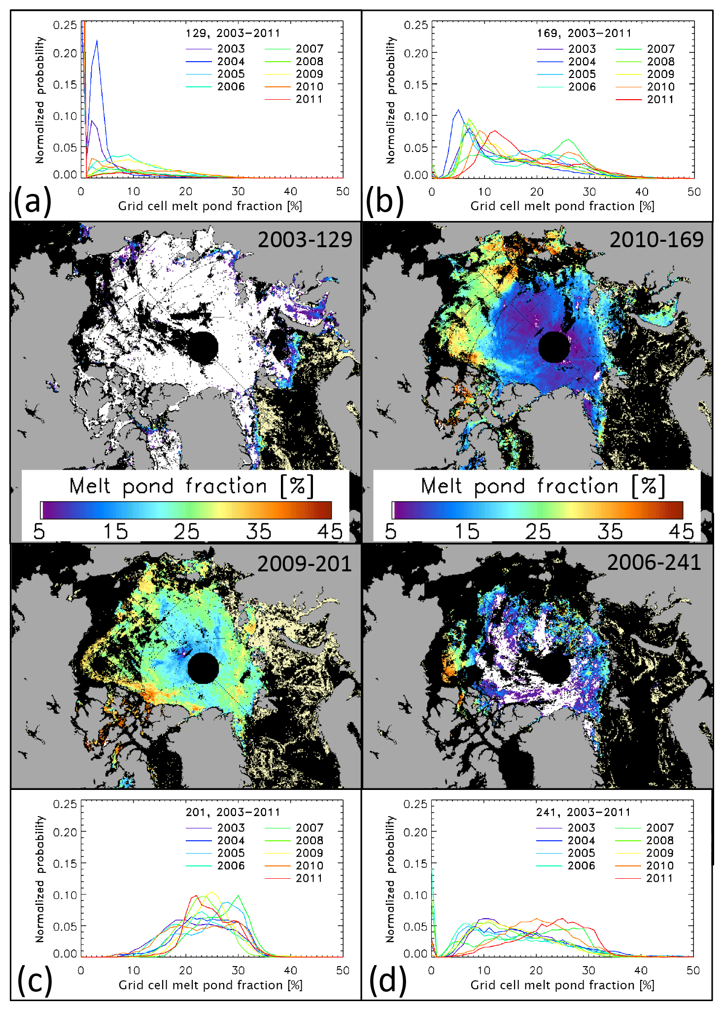
Figure 2 Sample maps of the Arctic melt pond fraction from the MODIS data set for (a) day of year (DOY) 129 (9–16 May) 2003, (b) DOY 169 (18–25 June) 2010, (c) DOY 201 (20–27 July) 2009, and (d) DOY 241 (29 August–5 September) 2006, illustrating the conditions during pre-melt, melt advance, peak melt, and end of melt, respectively. Black denotes open water, missing (note in this context the curvilinear one-grid-cell-wide features with missing data which originate from the gridding process) or invalid data, and clouds. Melt pond fractions smaller than 5 % are displayed in white. The histograms show the distribution of the melt pond fraction for the above-quoted DOY for every year of the period 2003–2011.

In Fig. 2 we illustrate the melt pond development in the Arctic Ocean as relevant for this paper. The maps show melt pond distributions of a DOY representative of the four periods considered in this paper: pre-melt, melt advance, peak melt, and end of melt in the maps of Fig. 2a–d, respectively. For these maps, we selected years where the data coverage is particularly good, i.e. with only a few grid cells discarded as potentially cloud contaminated. Below each map we show histograms of the melt pond fraction of the respective DOY of the years 2003 to 2011, to illustrate the inter-annual variability.

3 Pan-Arctic summertime sea-ice conditions

We begin our inter-comparison with an illustration of the sea-ice conditions in the Arctic during summer as seen by the satellite products. For this step, we compute an ensemble multi-annual (2002–2011) median of the monthly mean sea-ice concentration from the 10 sea-ice concentration products and subtract it from the respective sea-ice concentration of the individual product. This computation is carried out at 50 km grid resolution using a common land mask (see Kern et al., 2019). In Fig. 3 we show the differences between the products representative of groups I to IV (see end of Sect. 2.1) and the ensemble median as an example for the month of July (Fig. 3a–d) along with a map of the ensemble median sea-ice concentration (Fig. 3e). Figure 3 illustrates considerable differences between the four groups. Sea-ice concentration differences for July are particularly negative (mean sea-ice concentration smaller than ensemble median) for group III and particularly positive (mean sea-ice concentration larger than ensemble median) for group II. We refer to Fig. S4 in the Supplement for difference maps of all 10 products.

Differences between the individual products' multi-annual pan-Arctic monthly mean sea-ice concentration and the ensemble median increase from winter (Table 2, top row, January–February) to summer (Table 2, bottom row, July–August). Group I products show less sea ice than the ensemble median; group II and group IV products show more sea ice than the ensemble median; this applies to winter and summer. The absolute sea-ice concentration differences between the individual products and the ensemble median mostly increase from winter to summer.

These findings document, together with the results presented and discussed in Kern et al. (2019, Fig. 11 and Appendix G), that the 10 PMW SIC distributions differ considerably in summer. These findings agree with results from previous inter-comparisons of PMW SIC products (e.g., Comiso et al., 2017; Ivanova et al., 2014, 2015; Spreen et al., 2008; Meier, 2005).

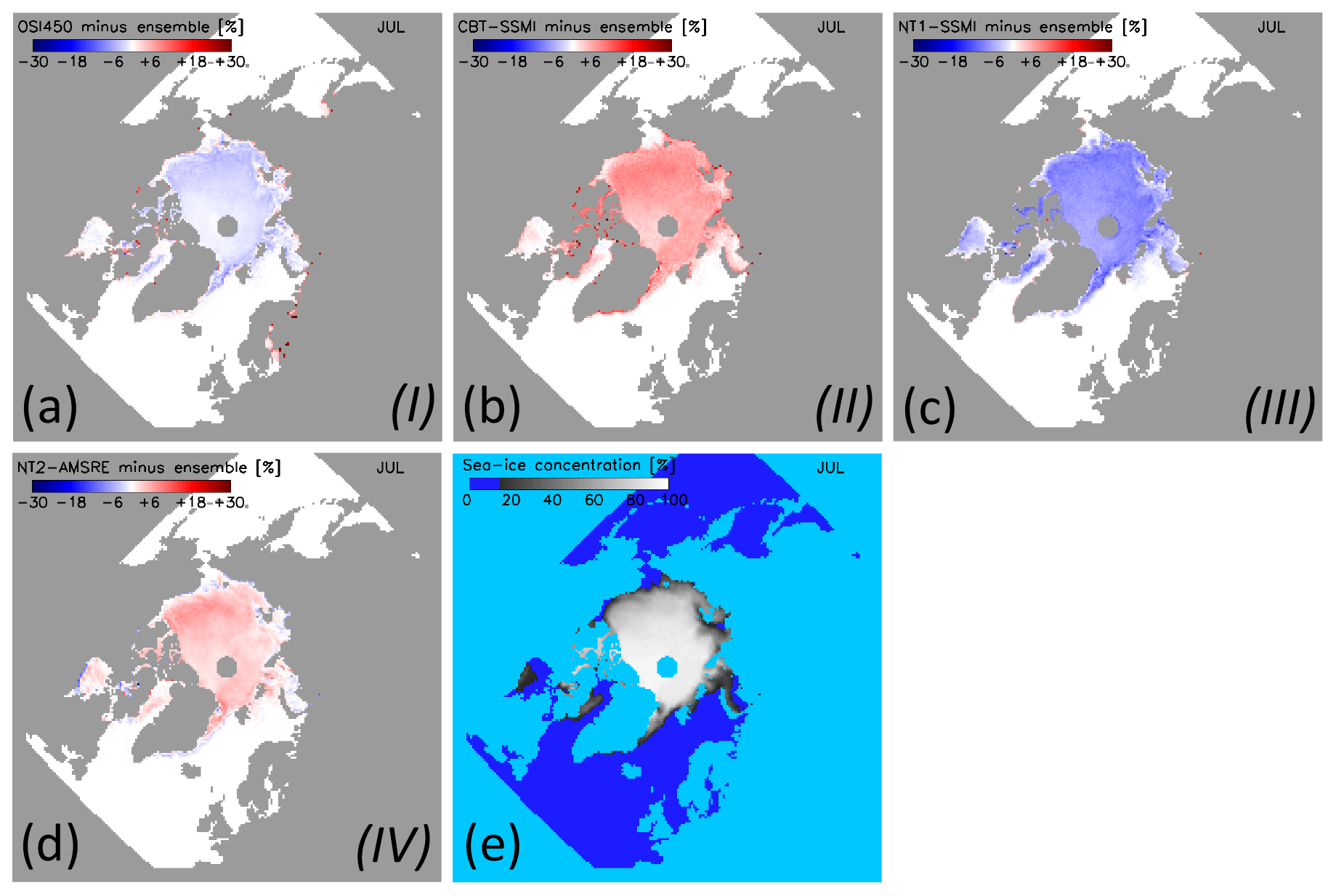
Figure 3 (a–d) Maps of the difference between the multi-annual average monthly SIC of the individual algorithms representing groups I to IV and the 10-algorithm ensemble median multi-annual average monthly SIC (e) for the Arctic for July 2003–2011 (see also Fig. S4, Supplement). Differences are only computed for sea-ice concentration of both data sets larger than 15 %. Roman numbers in bold font denote the group (see Table 1) to which the algorithm is assigned.

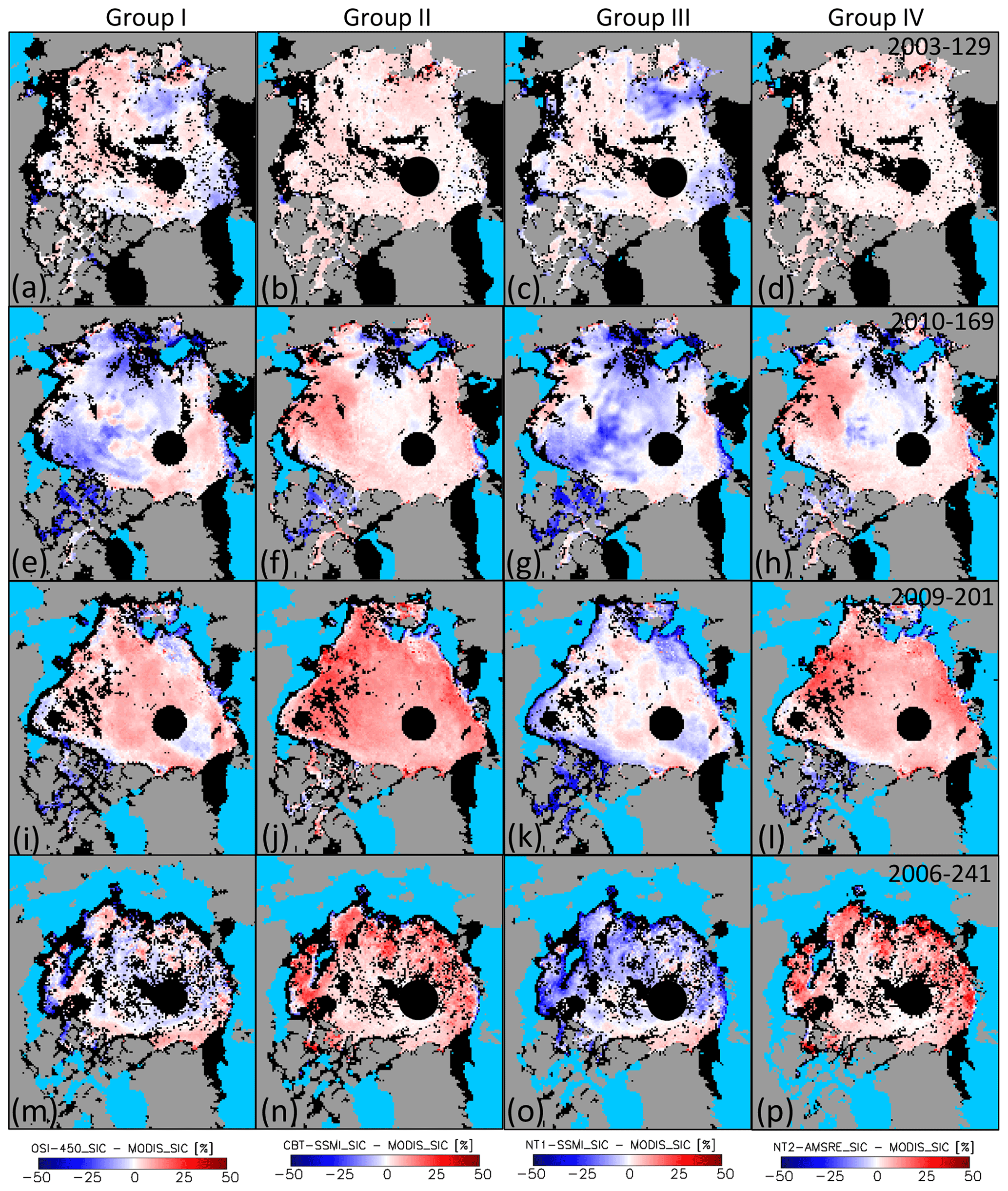
Figure 4 Maps of the difference of PMW minus MODIS sea-ice concentration for (a–d): day of year (DOY) 129 (9–16 May) 2003, (e–h) DOY 169 (18–25 June) 2010, (i–l) DOY 201 (20–27 July) 2009, and (m–p) DOY 241 (29 August–5 September) 2006; these are the same periods as used in Fig. 2. The leftmost column shows OSI-450, representing group I; the second column CBT-SSMI, representing group II; the third column NT1-SSMI, representing group III; and the rightmost column NT2-AMSR-E, representing group IV. Black areas denote invalid or missing data, clouds, or grid cells that are ice covered but not considered further in the analysis, e.g. in the Greenland Sea or Hudson Bay. The row starting with (a) is representative of pre-melt, the row starting with (e) is melt advance, the row starting with (i) is at the peak of melt, and the row starting with (m) is at the end of melt.

Table 2 Overall mean difference: individual algorithm SIC minus ensemble mean SIC in percent ice concentration for the Arctic for winter (months January and February) and summer (months July (see Fig. 3) and August). N denotes the total number of valid data pairs with SIC > 15.0 % (see also Kern et al., 2019).

4 Results

4.1 Inter-comparison against MODIS sea-ice concentration (SIC)

Figure 4 exemplifies how the difference of PMW SIC minus MODIS SIC changes as a function of the stage of melt for the four groups. For this illustration, we select the same 8 d periods as used in the maps shown in Fig. 2. The four rows represent stages of melt: pre-melt (DOY 129, 9–16 May), melt advance (DOY 169, 18–25 June), peak melt (DOY 201, 20–27 July), and end of melt (DOY 241, 29 August–5 September). The four columns represent groups I to IV by showing results of OSI-450 (group I), CBT-SSMI (group II), NT1-SSMI (group III), and NT2-AMSR-E (group IV). These examples are taken from different years, chosen because of a relatively small number of invalid or missing data. Figure 5 shows two-dimensional (2-D) histograms of PMW SIC (y axis) versus MODIS SIC (x axis) corresponding to the SIC maps used for the differences shown in Fig. 4. Note the logarithmic scale of the count. Similar histograms but based on SIC data of the years 2003 to 2011 are shown in Fig. S5 in the Supplement. We omit the pre-melt examples in Fig. 5 (and Fig. S5) because they exhibit limited additional information but show them for completeness in Fig. S6 in the Supplement.

4.1.1 Pre-melt

For the pre-melt example (Fig. 4a–d), only groups I and III exhibit notable areas of larger over- and underestimation of MODIS SIC (Fig. 4a, c), e.g. north of the Laptev Sea and the Fram Strait where group III exhibits negative differences above 15 % in magnitude. Apart from these patches of larger differences we can state that for pre-melt PMW SIC and MODIS SIC mostly agree within their uncertainties.

4.1.2 Melt advance

For the melt advance example (Fig. 4e–h), all four groups overestimate MODIS SIC by 5 %–10 % south of the pole facing Greenland and the Greenland, Barents, and Kara seas. In most other regions, MODIS SIC is either underestimated, e.g. in much of the central Arctic Ocean (Fig. 4e, g), or overestimated, e.g. in the Beaufort and Chukchi seas (Fig. 4f, h). Absolute differences remain mostly below 15 %. At this stage, melt has commenced everywhere and we observe a range of MPF values (see Fig. 2b). However, we find no unique correspondence between SIC differences and the MPF. On the one hand, MPF values below 15 % (Fig. 2b) correspond well to areas with only small absolute differences for groups II and IV (Fig. 4f, h). On the other hand, near-0 % differences between PMW SIC and MODIS SIC co-exist with MPF values ranging from below 10 % to above 30 % for the same groups. Likewise, for groups I and III, the spatial variability of SIC differences in the central Arctic Ocean (Fig. 4e, g) is not reflected by the spatial variability in the MPF (Fig. 2b). The above-mentioned differences between groups I and III on the one hand and groups II and IV on the other hand are also evident in the 2-D histograms matching the maps of Fig. 4e–h (Fig. 5, left column). Over the period 2003–2011 (Fig. S5, left column, Supplement), all four groups have the majority of SIC value pairs concentrated at values above 90 %. The differences in the distribution of the SIC value pairs between the groups are well reflected in the slight differences in linear regression line slope and intercept.

4.1.3 Peak melt

For the peak melt example, groups II and IV overestimate MODIS SIC almost everywhere by up to 20 % (Fig. 4j, l). This overestimation is confirmed well by the respective 2-D histograms (Fig. 5e, k). Regions with only 5 % to 10 % overestimation of MODIS SIC by these groups correspond to a range of different MPF values: up to 15 % in the central Arctic Ocean, around 30 % in the southern Beaufort Sea, and 40 % in the Canadian Arctic Archipelago (see Fig. 2c). Spatial patterns of SIC differences of groups I and III (Fig. 4i, k) are relatively similar to each other but differ considerably from those of the other two groups. We find that of all groups, group I has the highest linear correlation (0.84) and the smallest root-mean-squared difference (RMSD) of 7.8 % between PMW SIC and MODIS SIC (see Fig. 5, middle column). Over the period 2003–2011 (Fig. S5, middle column, Supplement), groups I and III provide a quite symmetric distribution with linear correlations of 0.86 and 0.87, respectively. For the other two groups, overestimation of MODIS SIC dominates – in agreement with Fig. 4j and l. Even though the linear correlation of 0.85 of group II is as high as those of groups I and III, the distribution of values suggests two separate linear regressions.

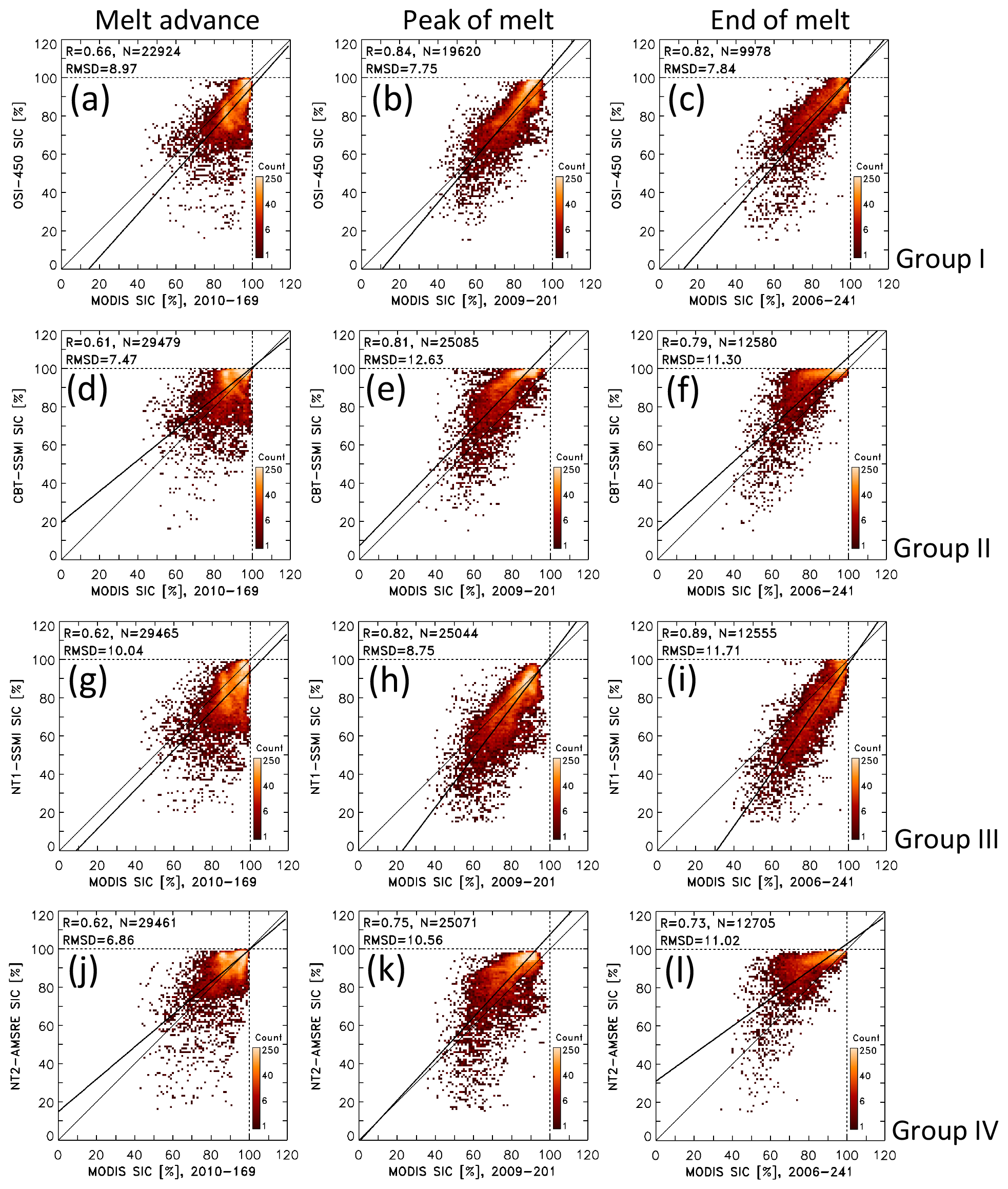
Figure 5 Two-dimensional histograms of the distribution of PMW (y axis) versus MODIS (x axis) SIC data pairs using a bin size of 1 % for the same 8 d periods as shown in Fig. 4e–p, i.e. melt advance, peak melt, and end of melt. The topmost row shows OSI-450 (for group I), the second row CBT-SSMI (for group II), the third row NT1-SSMI (for group III), and the bottommost row NT2-AMSR-E (group IV). The thin black line is the identity line. The thick black line denotes the linear regression through the data pairs. At the top left of every image we display the linear correlation coefficient R, the number of data pairs N, and the root-mean-squared difference RMSD; the latter is given in percent. The leftmost, middle, and rightmost columns represent melt advance, peak of melt, and end of the melt, respectively. Respective scatter plots for pre-melt are shown in Fig. S6 in the Supplement.

4.1.4 End of melt

For the end-of-melt example, spatial patterns of MODIS SIC overestimation by groups II and IV are very similar (Fig. 4n, p) as are the respective 2-D histograms (Figs. 5f, l and S5f, l, Supplement). MODIS SIC overestimation is largest where the melt pond fraction is largest and vice versa (compare with Fig. 2d) – except in the southern Beaufort Sea. Overall, group I has the smallest differences to MODIS SIC (Fig. 4m), the most symmetric SIC distribution around the identity line (Fig. 5c), and the smallest RMSD of 7.8 % of all groups. Over the period 2003-2011 (Fig. S5, right column, Supplement), group I and also group III have a quite symmetric SIC distribution, similar to peak melt.

Table 3 Average values of linear correlation, root-mean-squared difference (RMSD), and slope as well as intercept of the linear regression between passive microwave and MODIS sea-ice concentration for product groups I to IV (see text for further information). The averages are derived as the arithmetic mean from all 8 d period values of products within one group falling into pre-melt: DOY 129, 137, and 145, melt advance: DOY 153 to 185, peak melt: DOY 193 to 233, and end of melt: DOY 241 and 249.

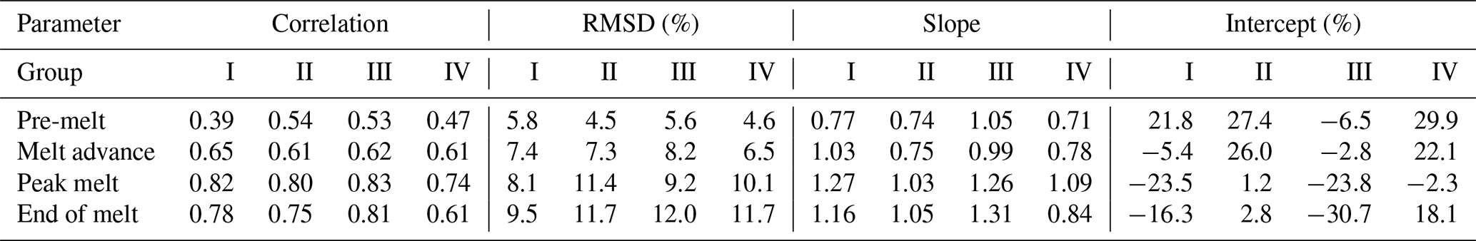
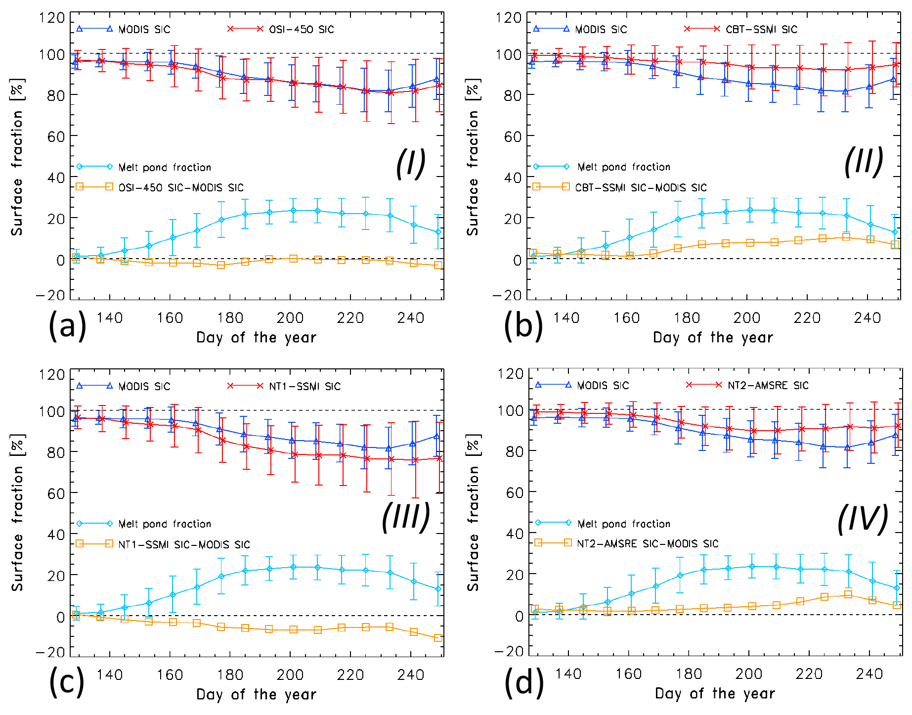
Figure 6 Average seasonal cycle of the mean (limited to Arctic Ocean and Canadian Arctic Archipelago) MODIS SIC (in blue), PMW SIC (in red), their difference of PMW minus MODIS SIC (in orange), and the MODIS melt pond fraction (in cyan), averaged for each 8 d period for the years 2003–2011 of the PMW products representing groups I to IV (see also Fig. S7, Supplement). Error bars denote 1 standard deviation of the mean. Roman numbers in bold font denote the group (see Table 1) to which the algorithm is assigned.

4.1.5 Summary of the comparison to MODIS SIC

We summarize the average values of the statistical parameters: regression line slope and intercept (or offset), linear correlation, and RMSD in Table 3. The averages are computed separately for the four stages of melt as the arithmetic mean over all parameter values of the respective group's products and 8 d periods within the years 2003 to 2011. For example, for the average RMSD of group I for pre-melt, we average over four (products in group I) times three (three 8 d periods within pre-melt: DOY 129, 137, and 145) times nine (years) values. We do not further interpret the values given for pre-melt and refer the reader to Figs. S6 and S9 in the Supplement. Table 3 shows an increase in correlation, RMSD, and slope from melt advance to peak melt for all four groups. Overall, the highest correlations between PMW SIC and MODIS SIC are obtained for groups I and III: 0.75 as a mean over melt advance to end of melt. If we take the RMSD as a measure of how accurate PMW SIC matches MODIS SIC, group I products are the most accurate ones with a mean RMSD from melt advance to end of melt of 8.3 %.

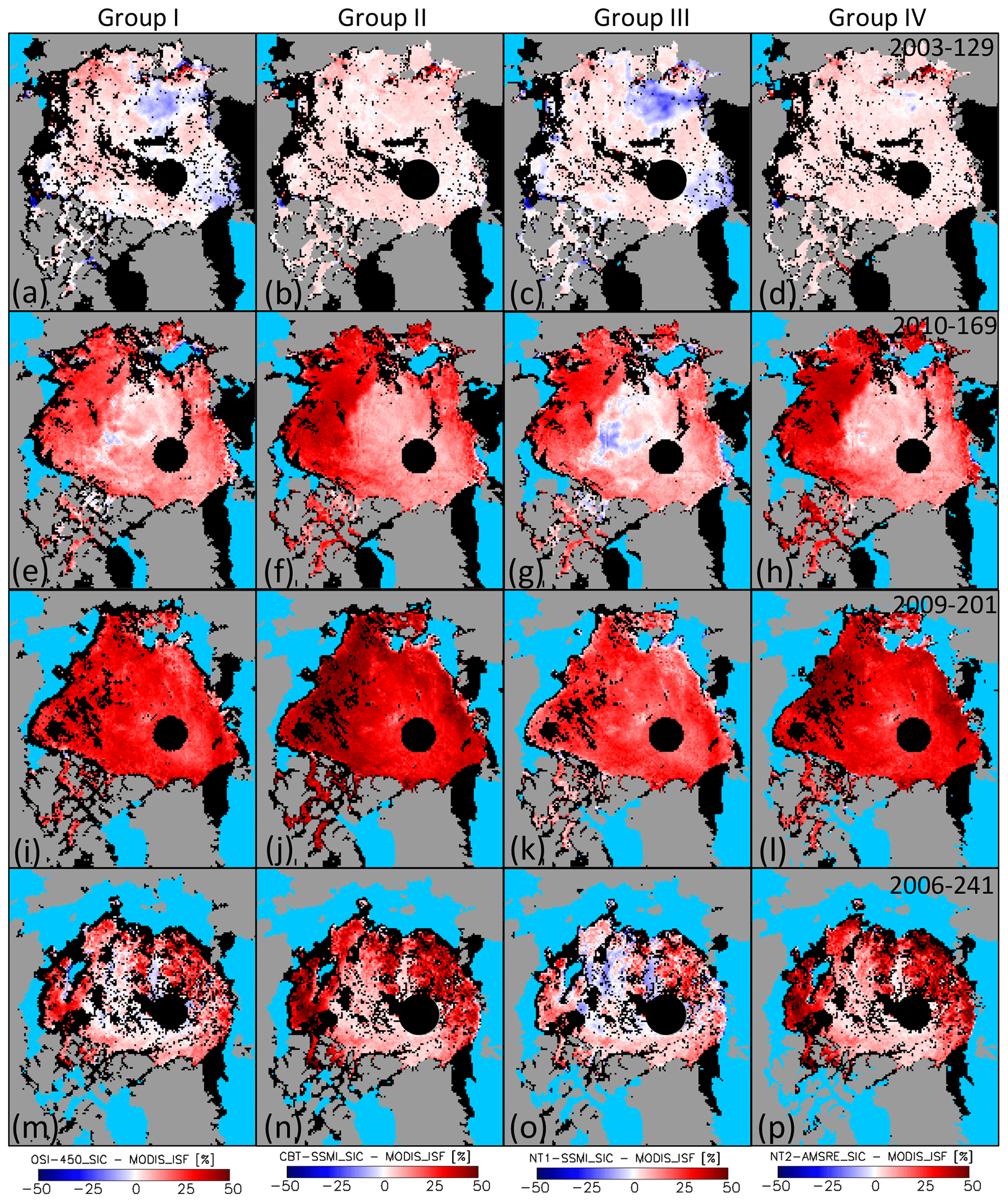
Figure 7 Maps of the difference PMW sea-ice concentration minus MODIS ice surface fraction (ISF) for the same 8 d periods as shown in Fig. 4. The leftmost column shows OSI-450, representing group I; the second column CBT-SSMI, representing group II; the third column NT1-SSMI, representing group III; and the rightmost column NT2-AMSR-E, representing group IV. Black areas denote invalid or missing data, clouds, or grid cells being ice-covered but not considered further in the analysis, e.g. in the Greenland Sea or Hudson Bay. The row starting with (a) is representative of pre-melt, the row starting with (e) is melt advance, the row starting with (i) is at the peak of melt, and the row starting with (m) is at the end of the melt.

Figure 6 summarizes our results about the pan-Arctic (Arctic Ocean and Canadian Arctic Archipelago) multi-annual mean melt season development of PMW SIC of the four products representative of the four groups in comparison to MODIS SIC and MPF. We refer to Fig. S7 in the Supplement for results of all 10 products. Temporal sampling is 8 d. The mean MODIS MPF is smaller than 5 % until the end of May (pre-melt), gradually increasing (melt advance) to a mean MPF of 20 %–25 % between DOY 180 and DOY 235, i.e. between the end of June and the third and fourth weeks of August (peak melt). We find near-0 % differences between PMW SIC and MODIS SIC for group I (Fig. 6a, orange symbols). These result from positive and negative biases cancelling out (see Figs. 4, 5b and S5, Supplement). Group II (Fig. 6b) exhibits near-0 % differences until the end of June but shows up to 10 % more sea ice than MODIS afterwards. Group III (Fig. 6c) first exhibits differences close to zero but shows less sea ice than MODIS during peak melt.

Of the four groups of products investigated, we get three different kinds of agreement between PMW SIC and MODIS SIC. Most importantly, instead of the underestimation commonly reported in the literature (e.g. Rösel et al., 2012b; Comiso and Kwok, 1996; Steffen and Schweiger, 1991; Cavalieri et al., 1990), our results suggest that an overestimation of the actual sea-ice concentration is common for several PMW SIC products. With that this study agrees with the findings in Kern et al. (2016), but we note that the latter study is based (i) on data of one summer season only; (ii) on data of a sub-region of the Arctic Ocean only; and (iii) on PMW SIC values computed from re-implementations of PMW SIC algorithms using fixed winter ice tie points and allowing SIC values larger than 100 %.

4.2 Inter-comparison against MODIS net ice surface fraction (ISF)

Melt ponds have the largest impact on PMW SIC because of the inability – at the microwave frequencies used – to discriminate between open water in the form of melt ponds on the ice floes and open water in the form of leads and openings between the ice floes. As detailed in the introduction, based on physical principles a sea-ice concentration retrieval algorithm should provide a value of 60 % for a case A, 100 % sea-ice concentration with 40 % melt ponds, and a case B, 75 % sea-ice concentration with 15 % melt ponds; in other words the algorithm should provide the net ice surface fraction. Therefore, a logical next step to better understand the causes of the SIC differences reported in Sect. 4.1 is to investigate how PMW SIC compares to ISF, as derived, e.g., from MODIS (Sect. 2.2). The inter-comparison between PMW SIC and MODIS ISF is carried out similarly to the inter-comparison to MODIS SIC (Sect. 4.1). We organize the results in exactly the same structure as in Sect. 4.1. We present in Fig. 7 a set of maps of the differences of PMW SIC minus MODIS ISF for the previously selected 8 d periods (compare Fig. 4), complemented by the respective 2-D histograms shown in Fig. 8 (compare Fig. 5) and extended to the entire period 2003–2011 in Fig. S8 in the Supplement (compare also Fig. S5).

4.2.1 Pre-melt

For the pre-melt example (Fig. 7a–d), almost no melt ponds are observed in the Arctic Ocean (see Fig. 2a); MODIS ISF equals MODIS SIC. The maps of the differences of PMW SIC minus MODIS ISF shown in Fig. 7a–d are almost identical to the maps shown in Fig. 4a–d. The differences between the 2-D histograms of this example are small, but when considering the entire period 2003–2011 we observe a tail of near-100 % PMW SIC values which spread over a range of MODIS ISF values between 60 %–70 % and 100 % (compare Figs. S6 and S9, left with right column, Supplement). The values in this tail are from locations where MODIS ISF is smaller than MODIS SIC and PMW SIC overestimates MODIS ISF, e.g. in the Laptev Sea and the East Siberian Sea (Fig. 7a–d). At these locations MPF is ∼ 10 % (Fig. 2a).

4.2.2 Melt advance

For the melt advance example (Fig. 7e–h), we find widespread overestimation of MODIS ISF by all groups. The highest overestimations occur in the Chukchi and Beaufort seas: up to 25 % for groups I and III (Fig. 7e, g) and up to 35 % for groups II and IV (Fig. 7f, h). North of this region an area extending across the Arctic Ocean towards Fram Strait has the smallest overestimation of MODIS ISF. Overall, the spatial pattern of the differences of PMW SIC minus MODIS ISF matches reasonably well with the respective MPF map (Fig. 2b). For example the area with differences ≤ 10 % in the central Arctic Ocean coincides with a MPF of ∼ 10 %. However, areas with the highest overestimation of MODIS ISF (e.g. by groups II and IV) do not necessarily coincide with the highest MPF. We get back to this issue in Sect. 5.1. The respective 2-D histograms reveal a bimodal distribution of the value pairs and magnitude of counts, which is similar for groups I and III (Fig. 8a, g) on the one hand and groups II and IV (Fig. 8d, j) on the other hand – like we found in Sect. 4.1 for MODIS SIC. The locations of the modes agree well with the differences shown in Fig. 7e–h. The findings from Fig. 8, left column, appear to be typical for the entire period 2003–2011 as illustrated by the 2-D histograms shown in Fig. S8, left column, in the Supplement.

4.2.3 Peak melt

For the peak melt example (Fig. 7i–l), PMW SIC overestimates MODIS ISF everywhere. The spatial distribution of the differences of PMW SIC minus MODIS ISF matches relatively well with the observed MPF (Fig. 2c). The overestimation is particularly high for group II (Fig. 7j): 20 %–25 % in the central Arctic Ocean and up to 45 % in the Chukchi and Beaufort seas. The overestimation is lowest for group III (Fig. 7k), 20 %–25 % in most areas, and is relatively homogeneous with respect to the SIC range as is evident in the respective 2-D histogram (Fig. 8h). This applies also for group I (Fig. 8b). Accordingly, the highest linear correlation coefficient and lowest RMSD values are obtained for groups I and III. The findings from Fig. 8, middle column, appear to be typical for the entire period 2003–2011 as illustrated by the 2-D histograms shown in Fig. S8, middle column, in the Supplement.

4.2.4 End of melt

For the end-of-melt example (Fig. 7m–p), we find reasonable agreement between the distribution of the MPF (Fig. 2d) and the difference of PMW SIC minus MODIS ISF for all groups. Areas of MPF less than 5 % coincide with differences between −10 % and 10 %. Areas with high MPF, however, do not necessarily coincide with areas of a large difference of PMW SIC minus MODIS ISF across the groups, as for instance the region with MPF of ∼ 35 % in the Beaufort Sea (Fig. 2d) for which we find differences between ∼ 15 % (Fig. 7o) and ∼ 40 % (Fig. 7n, p). The respective 2-D histograms (Fig. 8, right column) reveal very different relationships between PMW SIC and MODIS ISF for groups I and III on the one hand and groups II and IV on the other hand. When considering the entire period 2003–2011 (Fig. S8, right column, in the Supplement), values scatter much more and areas with high counts are much less confined than for the example shown in Fig. 8. This could be the result of (i) substantial inter-annual variation in the late summer co-existence and extent of melting and freezing conditions and of (ii) a larger uncertainty in the surface type classification in the MODIS product due to an unknown fraction of already refrozen melt ponds (see Sect. 2.2).

4.2.5 Summary of the comparison to MODIS ISF

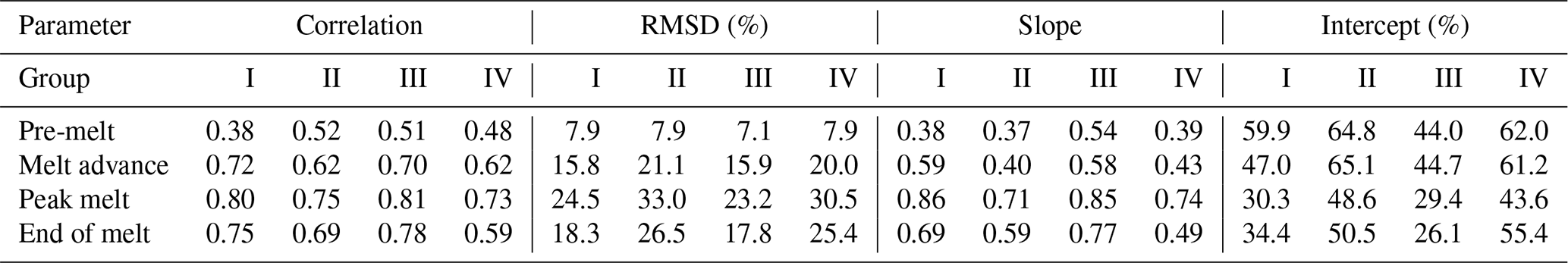
Values in Table 4 are computed similarly to those in Table 3 (see Sect. 4.1.5). They show an increase in mean values of correlation, RMSD, and slope from melt advance to peak melt for all four groups. Overall, we find the highest correlations between PMW SIC and MODIS ISF for groups I and III: 0.76 as the mean from melt advance to end of melt. For these groups, we also find the smallest mean RMSD values: 19.0 % and 19.5 % as the mean from melt advance to end of melt and 23.2 % and 24.5 % during peak melt. These values can be taken as a measure of MODIS ISF overestimation by PMW SIC. Slopes of the linear regressions get closest to 1 for groups I and III during peak melt, suggesting a solid linear relationship between PMW SIC and MODIS ISF – also in view of the distributions of values and counts in the 2-D histograms.

Agreement between the MPF and the magnitude of the difference of PMW SIC minus MODIS ISF differs among the four groups (compare Figs. 2 and 7). It appears that MODIS ISF is overestimated by group III by an amount smaller than the MPF while for groups II and IV the MODIS ISF overestimation is often larger than the MPF. This observation is confirmed by Fig. 9 (compare with Fig. 6). For group I (Fig. 9a), MPF values (in cyan) agree with the difference of PMW SIC minus MODIS ISF (in orange) within 2 % for the entire melt season. Hence, on a pan-Arctic scale, averaged over the years 2003 to 2011, group I products' overestimation of MODIS ISF equals the MPF. The overestimation of MODIS ISF by group II (Fig. 9b) and group IV (Fig. 9d) is larger than the MPF during peak melt and end of melt by up to 10 %, while for group III (Fig. 9c) this overestimation is smaller than the MPF by up to 10 %. We refer to Fig. S10 in the Supplement for results obtained for all 10 products.

We note in this context that we carried out an inter-comparison between ship-based visual sea-ice observations, providing independent estimates of SIC, MPF, and ISF, and all 10 products' SIC data. The results of this inter-comparison support our findings from Sect. 4.1 and this Section (see Sects. S1.1, S2.1 and Figs. S1 and S2 in the Supplement).

4.3 Bias correction as a potential way forward

The main motivations for this paper are to evaluate the performance of PMW SIC products during summer conditions and to better understand why PMW SIC products usually do not provide the net ice surface fraction – which they should following physical principles. The results presented so far document that none of the 10 PMW SIC products provide a faithful picture of the ISF, nor are they accurate measures of the summer SIC. The discussion given further below in Sect. 5 not only reveals possible explanations of the diversity of evaluation results but also demonstrates the complexity involved in a potentially planned improvement of the used algorithms – be it by further development of the algorithm itself or via application of more advanced ice tie point retrieval approaches. Here we discuss potential ways forward in the short to medium term (using existing PMW products) and in the longer term (preparing and using improved PMW SIC products).

For groups I and III, our comparison between PMW SIC and MODIS SIC (Sect. 4.1) and between PMW SIC and MODIS ISF (Sect. 4.2) suggests linear functional relationships. In the short term, these offer the prospect for users of the existing PMW SIC data sets from these two groups to perform bias corrections of the PMW SIC towards either true SIC (representative of the sea-ice area fraction of the geophysical model at hand) or net ISF (representative of the ice surface clear of melt ponds). The mean slope and intercept values prepared in Tables 3 and 4 but also slope and intercept of the individual linear regression lines (e.g. Figs. 5 and 8) could allow such a bias correction, noting all the limitations of these parameter values that are derived at pan-Arctic and, as presented in Tables 3 and 4, multi-year scales. For example, we find values of the linear correlation larger than 0.85 and slope close to 1 (see Table 4) with respect to MODIS ISF. With such a bias correction one might be able to get closer to the physically more meaningful result of a PMW SIC which equals the net ISF.

We do not explore or comment at length on a bias correction of PMW SIC towards true SIC with values in Fig. 5 (or Table 3). As predicted by physics, the bias correction towards true SIC is less skilled than towards net ISF, as can be assessed by the lower correlation values R in Fig. 5 (SIC) compared to Fig. 8 (ISF). A bias correction towards SIC would attempt to force the PMW SIC product to represent open water in two different ways: as sea ice when it is a melt pond and as true open water when it is a lead/opening between the ice floes, despite the fact that the surface emissivity and hence the observed TB are determined by the overall total amount of liquid water at the surface.

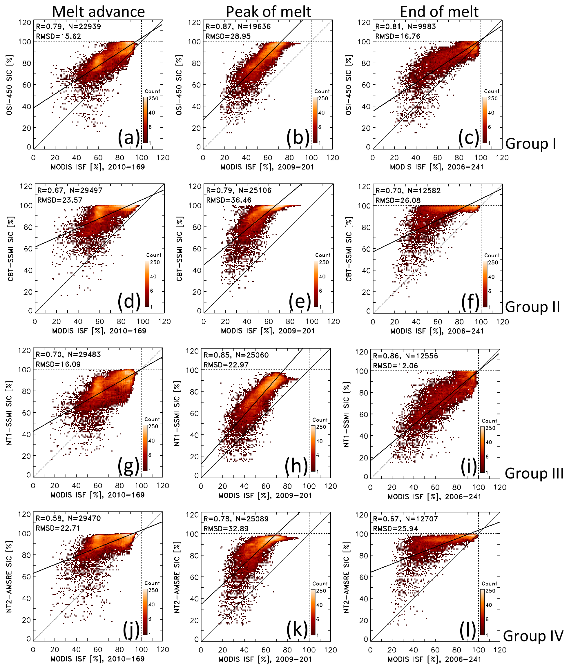
Figure 8 Two-dimensional histograms of the distribution of PMW SIC (y axis) versus MODIS ISF (x axis) data pairs using a bin size of 1 % for the same 8 d periods as shown in Fig. 7e–p, i.e. melt advance, peak melt, and end of melt. Panels (a–c) show OSI-450 (for group I), (d–f) CBT-SSMI (for group II), (g–i) NT1-SSMI (for group III), and (j–l) NT2-AMSR-E (group IV). The thin black line is the identity line. The thick black line denotes the linear regression through the data pairs. At the top left of every image we display the linear correlation coefficient R, the number of data pairs N, and the root-mean-squared difference (RMSD); the latter is given in percent. The leftmost, middle, and rightmost columns represent melt advance, peak of melt, and end of the melt, respectively. Respective scatter plots for pre-melt are shown in Fig. S9 in the Supplement.

Table 4 Mean values of linear correlation, root-mean-squared difference (RMSD), and slope as well as intercept of the linear regression between passive microwave sea-ice concentration and MODIS ice surface fraction for product groups I to IV (see text and caption of Table 3 for further information).

We hence only use linear regression equations obtained from the comparison between PMW SIC and MODIS ISF for a bias correction of PMW SIC towards MODIS ISF. We first test how well the bias correction works in comparison to MODIS ISF, i.e. investigate whether the difference between PMW SIC and MODIS ISF is reduced to zero, and subsequently compare the bias-corrected PMW SIC to MODIS SIC. This bias correction is exemplarily carried out for OSI-450 (group I), CBT-SSMI (group II), and NT1-SSMI (group III) for peak melt (DOY 201, year 2009) in Fig. 10 and for melt advance (DOY 169, year 2010) in Fig. S11 in the Supplement. Note that we use slope and intercept values obtained exactly for these examples, i.e. from Fig. 8, and not from Table 4.

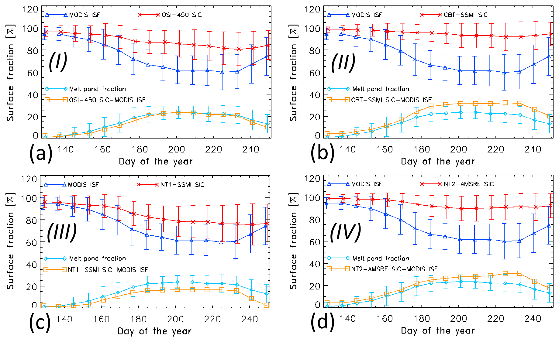
Figure 9 Average seasonal cycle of the mean (limited to Arctic Ocean and Canadian Arctic Archipelago) MODIS ISF (in blue), PMW SIC (in red), their difference of PMW SIC minus MODIS ISF (in orange), and the MODIS melt pond fraction (in cyan), averaged for each 8 d period over the years 2003–2011 of the PMW products representing groups I to IV (see also Fig. S10 in the Supplement). Error bars denote 1 standard deviation of the mean. Roman numbers in bold font denote the group (see Table 1) to which the algorithm is assigned.

The bias correction works well with respect to MODIS ISF for peak melt. The majority of the differences of bias-corrected PMW SIC minus MODIS ISF have a magnitude less than 5 % (Fig. 10d–f). The linear correlations are as high as for the uncorrected case and the RMSD decreases to around 6 %–7 % (compare Fig. 10a–c with Fig. 8b, e, h); the slope is almost identical to the identity line for OSI-450 and NT1-SSMI. We note that if the results of this bias correction prove to be of equal quality for other parts of the peak-melt period and other years, one could use the respective equations to obtain an independent estimate of the ISF from the entire PMW SIC data record, i.e. from 1979 to today. This could serve as an important boundary condition for the estimation of the surface albedo independent of daylight and cloud cover, complementing existing data sets and aiding in their evaluation (e.g. Riihela et al., 2010, 2017). For melt advance (Fig. S11a–f, Supplement), differences between bias-corrected PMW SIC and MODIS ISF are considerably larger than for peak melt, especially for CBT-SSMI and NT1-SSMI. While the slopes all agree quite well with the identity line, RMSD values are much larger than for peak melt. This is also evident from the larger scatter of value pairs in the respective 2-D histograms. During melt advance it appears advisable to use non-truncated SIC values if available, because the fraction of SIC larger than 100 % is the highest during the summer melt cycle (see Sect. S3.1 in the Supplement); at this stage we did, however, not further quantify the effect this may have on the results of the bias correction performed.

As expected, the difference of bias-corrected PMW SIC minus MODIS SIC is negative all over and has a magnitude of about 25 %. We find a relatively homogeneous distribution of differences (Fig. 10j–l). We find value pairs in the respective 2-D histograms to be confined below the identity line around a linear regression line with a slope slightly larger than 1 and linear correlations comparable to the uncorrected PMW SIC (Fig. 5b, e, h). Most striking is the similarity of the distributions in the maps and 2-D histograms across the three products and the fact that the RMSD between bias-corrected PMW SIC and MODIS SIC not only agrees within 1 % among the three products but also agrees with the modal MPF of 25 % for DOY 201 of the year 2009 (see Fig. 2c). Thus, the bias correction towards ISF reconciles the various PMW SIC products towards a consistent difference of PMW SIC minus MODIS SIC of the same order of magnitude as the average MPF. In contrast, during melt advance with melting and frozen and wet and dry surfaces co-existing, the results of the bias correction of PMW SIC appear less convincing (Fig. S11g–l, Supplement). Here CBT-SSMI provides a difference bias-corrected PMW SIC minus MODIS SIC, which in the central Arctic Ocean is uniform at about 10 %. While this value matches well with the MPF map and the first mode (9 %) of the bimodal MPF distribution for DOY 169 of the year 2010 (Fig. 2b), the other differences range between −40 % and 10 %, demonstrating that during melt advance a bias correction as proposed is potentially of limited value.

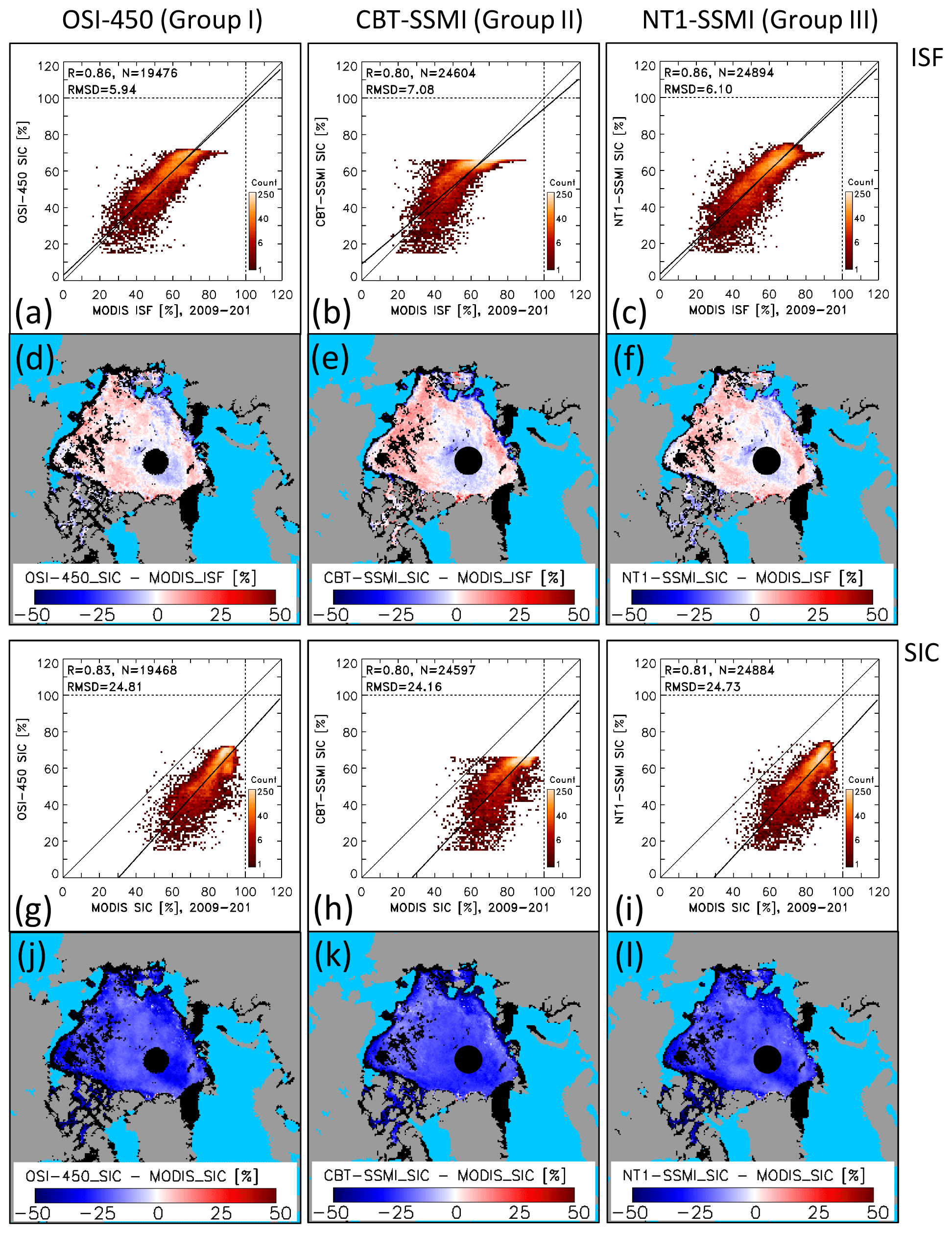
Figure 10 Illustration of the effect of a simple linear bias correction of PMW SIC towards MODIS ISF for an 8 d period during peak melt (DOY 201, 20–27 July 2009). (a–c) Two-dimensional histograms of the distribution of bias-corrected PMW SIC (y axis) versus MODIS ISF (x axis) data pairs. (d–f) Respective maps of the difference of bias-corrected PMW SIC minus MODIS ISF. (g–i) Two-dimensional histograms of the distribution of bias-corrected PMW SIC (y axis) versus MODIS SIC (x axis) data pairs. (j–l) Respective maps of the difference of bias-corrected PMW SIC minus MODIS SIC. The leftmost, middle, and rightmost columns show OSI-450 (for group I), CBT-SSMI (for group II), and NT1-SSMI (for group III). Bin size in the histograms is 1 %. The quantities given in the top left corner are R: linear correlation coefficient, N: number of valid data pairs, and RMSD: root-mean-squared difference. The thin black line is the identity line; the thick black line denotes the linear regression through the data pairs.

A logical next step would be to use the mean values of slope and intercept (Table 4) instead of the individual values (see above). We note that the mean values (Table 4) differ considerably from the individual values. For example, for OSI-450 during the 8 d period beginning at DOY 201 in year 2009 we have individual values of intercept and slope of 27.3 % and 1.01, respectively, while the respective mean values for group I during peak melt are 30.3 % and 0.86 (Table 4). We did not yet apply these, however, because we regard these first attempts as a feasibility study only. To carry out a comprehensive study about the potential of a bias correction of PMW SIC towards MODIS ISF would require a well-thought concept about how to adequately evaluate the bias-corrected SIC; this is beyond the scope of this paper.

After such a study, in the short term, values given in Table 4 could allow users of the existing PMW SIC data sets to bias-correct these products towards net ISF. Such a bias correction is however not necessarily useful in practice. Indeed, users must now rely on additional sources of information to link their SIC (e.g. from a geophysical model) to a measure of the ISF. This for example requires a trustworthy representation of the evolution of melt ponds on sea ice in their model. Several such melt pond schemes are being developed (e.g. Pedersen et al., 2009; Flocco et al., 2010; Scott and Feltham, 2010; Holland et al., 2012; Skyllingstad et al., 2015; Popović and Abbot, 2017), but their application and evaluation reveal some challenges remain (e.g. Light et al., 2015; Tsamados et al., 2015; Zhang et al., 2018; Burgard et al., 2020; Dorn et al., 2019). Still, in the long run, using PMW SIC as an observation of net ISF should be favoured, as it is more meaningful and will be more accurate. This will especially be the case when producers of PMW SIC data sets put additional effort into improving their algorithms and/or ice tie point selection schemes to actually retrieve unbiased observations of the net ISF. There is furthermore no doubt that both improving melt pond schemes in models and designing better PMW-based SIC algorithms in summer will benefit from better accuracy and availability of Earth-observation-based melt pond fraction CDRs from visible–infrared imager instruments such as NASA MODIS (e.g., Rösel et al., 2012), the European Space Agency's MEdium Resolution Imager Sensor (MERIS) (e.g., Istomina et al., 2015; Zege et al., 2015), or the Copernicus Ocean and Land Colour Imager (OLCI). There is a critical Earth observation (EO) gap to be filled here in order to further improve the Sea Ice essential climate variable (ECV).

4.4 The impact on sea-ice area

Independent of the way forward and future attempts to get closer to what appears to be physically more correct when using satellite PMW data for SIC retrieval, we note that there might be applications which require an accurate SIC including the melt ponds on top, i.e. without the need to understand why the PMW SIC does not match the actual net ISF. The classical application would be the computation of the SIA, the sum of the area of all ice-covered grid cells weighed by SIC. We demonstrated in Sect. 4.1 which groups over- and/or underestimate MODIS SIC where and by which amount (Figs. 4, 5 and S5, Supplement). We illustrated that on a pan-Arctic scale, averaged over the years 2003–2011, group I exhibits a near-0 % bias, while group III appears to underestimate MODIS SIC by 5 %–10 % during peak melt and end of melt, and group II appears to overestimate MODIS SIC by around 10 % (see Fig. 6). This finding holds for melt pond fractions up to 30 % and for NT1-SSMI and group II products even up to 40 % (Fig. 11a). In addition, Fig. 11b further illustrates how well the difference of PMW SIC minus MODIS ISF can be seen as a linear function of the MPF for group I – at least up to a MPF of ∼ 30 %.

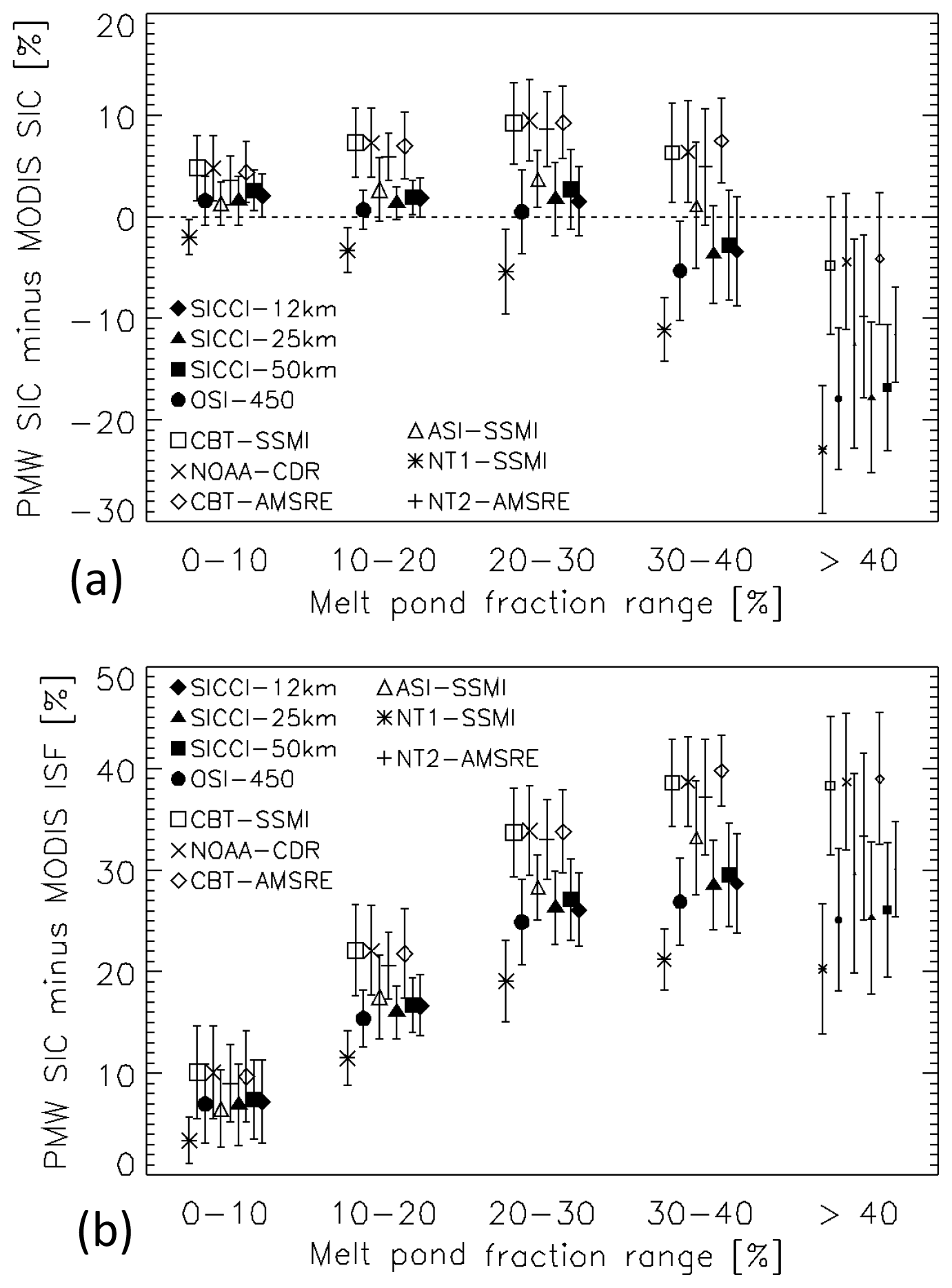
Figure 11 Mean difference of PMW SIC minus MODIS SIC (a) and PMW SIC minus MODIS ISF (b) derived for all 8 d periods of the years 2003–2011 for all 10 products separately for melt pond fraction ranges 0,%–10 % to > 40 %. Error bars denote 1 standard deviation of the mean. Symbol size scales with the number of valid data pairs. The topmost four and bottommost three entries in the left column of annotations denote group I (filled symbols) and group II, respectively. The topmost two entries and the last entry in the right column of annotations denote group III and group IV, respectively.

Coming back to the computation of SIA and the potential influence of melt ponds, as shown in Kern et al. (2019) and Ivanova et al. (2014), the choice of the product for the computation of SIA from PMW SIC data makes a difference. For the months July through September of the years 2002–2011, the SIA computed from PMW SIC of group I products is ∼ 400 000 km² larger than SIA computed from NT1-SSMI (group III) and ∼ 600 000 km² smaller than SIA computed from group II products (Kern et al., 2019, Fig. G2g–i). The average pan-Arctic MODIS SIC for these months is between 85 % and 90 % (Figs. 6 and S7, Supplement). Considering a value of 90 % and assuming an extent of 6 million square kilometres to be covered by some amount of sea ice on average for these months, we end up with a SIA of about 5.4 million square kilometres based on MODIS. Group I products, exhibiting zero bias to MODIS SIC (Figs. 6a, S07a–d) yield the same SIA estimate. NT1-SSMI, exhibiting a negative bias of 5 %–10 % (Figs. 6c, S7i), say 7 %, i.e. a pan-Arctic average SIC of 83 %, yields a SIA of 5.0 million square kilometres. Group II products, exhibiting a positive bias of ∼ 10 % (Figs. 6b, S7e–g), i.e. a pan-Arctic average SIC of 100 %, yield a SIA of 6.0 million square kilometres. Based on these considerations we can conclude that the summertime differences between the SIA estimates of the 10 products presented by Kern et al. (2019) can be explained well with the differences between PMW SIC and MODIS SIC presented in this paper.

5 Discussion and conclusions

5.1 Discussion

5.1.1 Understanding our observations

Our results demonstrate that the different products respond quite differently to the changes in the sea-ice cover during summer melt and that none of them are doing things quite right. This is not surprising given the variety of different sea-ice and snow physical properties relevant for satellite PMW sensing of sea ice – open and refrozen melt ponds, slush, saturated or wet snow, new snow, coarse-grained melting or refrozen snow, bare melting ice, bare dry ice, submerged ice, and various forms of new ice – co-existing during summer at the pan-Arctic scale but possibly even within one satellite footprint. These physical properties not only undergo substantial changes during the melt season, they also have a large spatio-temporal variability. The net surface energy balance driving the melting or freezing is very sensitive to variations in the cloud cover and to precipitation events, which can vary on short temporal and local spatial scales. Melting and refreezing of coarse-grained snow or formation of a thin ice cover at the melt pond surface can occur within a few hours.

Besides melt ponds, wet snow and melting and refrozen coarse-grained snow are the most relevant surface parameters. At the microwave frequencies used in this paper the emissivity of the wet snow cover is close to 1, resulting in a microwave TB close to 273.15 K – the melting temperature of snow. Typical increases in microwave TB due to an increase in snow wetness range between 10–15 and 60 K (Kern et al., 2016, Table 1). The magnitude of this TB increase depends on the sea-ice emissivity being a function of frequency and polarization. The increase is higher for multi-year than first-year ice. It is higher at horizontal (H) than vertical (V) polarization and at higher (near-90 GHz) than lower (19 GHz) frequency (f). This is all in accordance with the lower TB of multi-year ice than first-year ice and the lower TB at horizontal than vertical polarization of winter sea ice. Concomitant is a decrease in the normalized TB polarization difference: $\text{PR}\left(f\right)=\frac{{\text{TB}}_V\left(f\right)-{\text{TB}}_H\left(f\right)}{{\text{TB}}_V\left(f\right)+{\text{TB}}_H\left(f\right)}$, at a frequency of 19 GHz (PR19) or 89 GHz (PR89) as well as a decrease in the magnitude of normalized TB gradient ratios: $\text{GR}\left(f_{\mathrm{1}}{f}_{\mathrm{2}}\right)=\frac{{\text{TB}}_V\left(f_{\mathrm{1}}\right)-{\text{TB}}_V\left(f_{\mathrm{2}}\right)}{{\text{TB}}_V\left(f_{\mathrm{1}}\right)+{\text{TB}}_V\left(f_{\mathrm{2}}\right)}$, between 19 and 37 GHz (GR3719) or 19 and 89 GHz (GR8919), quantities that are used in the NT1-SSMI and NT2-AMSR-E algorithms (see Kern et al., 2019, for a summary of relevant technical aspects of the 10 algorithms used). Typical decreases in microwave TB due to an increase in snow grain size, e.g. due to surface refreezing or surface crust formation, are around 15–35 K (Kern et al., 2016, Tables 1 and 3). The magnitude of such a decrease is larger at horizontal than vertical polarization and larger at higher than lower frequencies. Concomitant is an increase in the magnitude of, e.g., PR19 and GR3719 by 0.02 and 0.05, respectively. Such increases correspond to about 10 % in SIC. Melting of a coarse-grained snow cover reverts the above-mentioned changes, causing diurnally changing microwave TB values should melt–refreeze cycles commence.

In summary, whenever the surface conditions become wetter, microwave TB increases, while polarization and frequency differences decrease. Whenever surface conditions become drier, microwave TB decreases, while polarization and frequency differences increase. This view is certainly a simplification of the true conditions which are more complex due to the vertical structure of the snow cover, the different near-surface properties of first-year ice compared to multi-year ice, melt pond drainage and other processes. However, this view allows us to understand that during summer, differences between an actually observed microwave TB or TB difference and an ice tie point can be caused by the mismatch between actual and tie point conditions with respect to the representation of (i) melt ponds; (ii) snow wetness, (iii) snow grain size and surface type, (iv) ice type, and (v) a mixture of all these.

The implications for the SIC retrieval depend on the type and update interval of the tie points of pure sea ice, i.e. 100 % sea-ice concentration (see e.g. Lavergne et al., 2019). The ASI algorithm (group III) uses one global fixed sea-ice tie point value (Kaleschke et al., 2001). NT1-SSMI (group III) uses one fixed set of fixed TB values for first-year ice and multi-year ice. NT2-AMSR-E (group IV) uses sets of 12 fixed TB values of all involved channels (see Table 1) of three different ice types: thin ice, ice type A (merges first-year and multi-year ice), and ice type C (sea ice with a thick snow cover). The 12 fixed TB values are based on the 12 different atmospheric states used to compute the look-up tables for the SIC retrieval (Markus and Cavalieri, 2009). All other products (groups I and II), except the contribution of NT1-SSMI to the NOAA CDR product, use an ice line which interpolates between signatures of first-year and multi-year ice and which is updated daily (Lavergne et al., 2019; Comiso and Nishio, 2008). For group I products this ice line is computed from TB measurements over closed ice within a moving 15 d interval centred at the day of the actual SIC retrieval; closed ice is defined as grid cells with more than 95 % NASA Team algorithm SIC. A post-processing step optimizes the location of the ice line with respect to the different TB values encountered as a function of ice type. The Comiso bootstrap algorithm (CBT-SSMI and CBT-AMSR-E) derives the ice line via linear regression analysis of the respective TB value cluster. This is done in both TB spaces, i.e. TB37V/TB37H used for SIC larger than 90 % and TB37V/TB19V used for SIC below or equal to 90 % (Comiso et al., 1997). The offset (or intercept) of the obtained linear regression line is increased by a few kelvin to account for the presence of some open water (2 %–3 %) in closed-ice areas (Comiso and Nishio, 2008; Comiso, 2009). These differences in the ice tie points already suggest that the different products represent the actual sea-ice conditions with different levels of accuracy. None, to our best knowledge, of the algorithms used in the 10 products employ regionally varying ice tie points notwithstanding the large spatial variability of the relevant physical properties during the melt season.

Example 1: pre-melt conditions

For all groups we observe small areas of elevated positive differences of PMW SIC minus MODIS ISF (Fig. 4a–d). These areas can be explained with the concurrent melt pond fraction. An influence by elevated snow wetness is unlikely, because this would cause an increase in PMW SIC which in turn would result in an overestimation of both MODIS SIC and MODIS ISF – which is not observed. However, groups I and III reveal patches of MODIS SIC and ISF underestimation (Fig. 4b, d; see also Figs. S7 and S10 in the Supplement) not found for the other groups. As one possibility these patches could be explained by a refrozen surface or coarse-grained snow not represented in the ice tie points. NT1-SSMI (group III) PMW SIC is based on PR19 and GR3719 and the above-mentioned surface conditions would cause an underestimation of the SIC (see Kern et al., 2016, Fig. 6a: respective data pairs would move away from the red ice line towards the open-water tie point). The algorithms of group I use NT1-SSMI SIC > 95 % as a priori information for the computation of the ice tie point (Lavergne et al., 2019). Grid cells with an actual near-100 % SIC, where such an underestimation by NT1-SSMI occurs under the mentioned surface conditions, are possibly excluded from the tie point estimation for group I algorithms. As a consequence such regions are not represented by the ice tie point, and we have a mismatch between actual and tie point conditions, and the retrieved SIC is biased low.

Example 2: melt conditions

We find cases where near-100 % MODIS SIC coincides with a near-0 % difference of PMW SIC minus MODIS SIC, an overestimation of MODIS ISF by 10 %–15 % and a MPF of 10 %–15 %, e.g. for CBT-SSMI (group II) in the central Arctic Ocean (Figs. 4f and 7f). One would expect that the open water associated with the melt ponds (non-zero MPF) lowers the actually observed TB and that therefore the actual PMW SIC is smaller than the MODIS SIC. This is not the case. We offer three explanations.

• Explanation A. The ice tie point includes some influence of melt ponds. In that case the ice tie point (see e.g. the ice line in Kern et al., 2016, Fig. 6c, d) would be located at a lower TB value slightly closer to the open-water tie point. The observed TB would then match with this ice tie point – provided that actual ice surface properties between the melt ponds match the conditions represented by the ice tie point – and the retrieved SIC would be close to 100 %. We hypothesize that this is one of the most likely reasons for the overestimation of MODIS ISF by group I products. These products use NT1-SSMI SIC > 95 % to define regions for ice tie point retrieval (Lavergne et al., 2019), regions which according to the results of our paper exhibit a non-zero melt pond fraction.

• Explanation B. The surface between the melt ponds is wet but this is not represented by the ice tie point. In that case the observed TB is lowered by the melt ponds but at the same time increased by the wet surface. Both effects could compensate for each other such that the observed TB is close enough to the ice tie point to yield near-100 % SIC. Evidence for an increase in TB during summer melt in June is given, e.g. in Kern et al. (2016, Fig. 8a–c); the cluster of increased TB values is located considerably above the wintertime ice line concomitant with near-100 % MODIS ISF (Kern et al., 2016, Fig. 6c).

• Explanation C. The ice tie point represents a refrozen surface or multi-year ice and because of this is located similarly closer to the open-water tie point as in explanation (A). The observed TB would match the ice tie point for the wrong reason and the algorithm would provide near-100 % SIC.

We find other cases where 100 % PMW SIC coincides with a MODIS SIC of 85 % and a melt pond fraction of 25 %–30 %, e.g. for CBT-SSMI (group II) in the Chukchi Sea (Figs. 4f and 7f). Here, despite the large open-water fraction of 40 %–45 %, PMW SIC is 100 %, which corresponds to an overestimation of MODIS SIC by 15 % and of MODIS ISF by 40 %–45 %. All explanations suggested in the previous paragraph might apply here – very likely in combination with each other. Such a large overestimation of MODIS ISF would, if we use only explanation B, require unphysical sea-ice surface emissivities larger than 1 (not shown). Using different algorithms Kern et al. (2016) computed the SIC based on elevated summertime microwave TB values. They found that – theoretically – SIC values would need to be as high as 140 % for the fraction of the grid cell not covered by water to explain their observed differences between PMW SIC and MODIS ISF for MODIS SIC values above 90 %. The way ice tie points are derived in the Comiso bootstrap algorithm suggests (i) inclusion of melt ponds in the tie point, (ii) unaccounted for wet snow/wet surface between the melt ponds and (iii) ice type mismatches to be the most likely combination leading to the observed overestimation.

Summary

The co-existence of different surface properties during summer adds complexity to the SIC retrieval using satellite PMW TB observations. Our attempts to explain the observations suggest that an adequate understanding of – on the one hand – the actually encountered sea-ice and snow properties and – on the other hand – the properties represented by the ice tie points is required. The influence exerted by different surface properties on the actually measured TB or TB differences like PR19 or GR3719 can cancel out. Examples of such properties are the co-existence of melting and refrozen coarse-grained snow or the co-existence of wet snow and melt ponds. A consequence of this is that despite the actual surface conditions not matching the ice tie point conditions, retrieved PMW SIC sometimes appears to be accurate. It needs to be better understood how ice tie points are derived during summer conditions and how their validity can be assessed as a function of location and time. Based on our findings, one of the largest issues could be the inclusion of an unknown amount of melt ponds into the ice tie point.

5.2 Conclusions

Following up on the release of three new global sea-ice concentration (SIC) climate data records (CDRs) described in Lavergne et al. (2019), this paper focuses on an inter-comparison of these three CDRs and seven other SIC products (see Kern et al., 2019) with estimates of the SIC and the net ice surface fraction (ISF) in the Arctic during summer (May through September) for the years 2003 through 2011 obtained from satellite observations by the MODIS sensor. The motivation for this dedicated paper is the fact that it is particularly challenging to derive the SIC of melting sea ice. It is impossible with the current microwave radiometer sensors to distinguish water in melt ponds on top of the sea ice from the water in the leads between the sea-ice floes. What we expect to measure with the microwave radiometer sensor is therefore the ISF even though this is not what scientists normally relate to the term “sea-ice concentration”. The ISF radiometric signature and especially its variability are difficult to characterize when the sea ice is melting and this results in large random and systematic uncertainties when retrieving the SIC and ISF from PMW observations. Our study employs 10 SIC products which we assign to four groups based on their retrieval algorithm (see Table 1) – like we did in our previous study (Kern et al., 2019). Our results document that none of the 10 PMW SIC products provide an accurate measure of the summer SIC, or a faithful picture of the ISF.

Overall we find group I products (SICCI and OSI-450; see Table 1) exhibit a near-0 % bias to the MODIS Arctic average SIC – independent of melt pond fractions up to ∼ 35 % (Fig. 11a). Group II (CBT-SSMI, CBT-AMSR-E and NOAA-CDR) and IV (NT2-AMSR-E) products have a positive bias of 5 %–10 %, and NT1-SSMI (group III) has a negative bias of 5 %–10 %. However, these small overall biases are the result of widespread, spatio-temporally varying positive and negative differences of substantial magnitude which cancel out in a pan-Arctic mean for some of the products. Magnitudes of these biases frequently reach up to 20 %–25 % for groups I and III and up to 30 %–35 % for groups II and IV. Unlike what is generally accepted and reported in the literature, we observe that several PMW SIC products significantly overestimate true SIC.

By comparing PMW SIC with MODIS ISF and the MODIS melt pond fraction (MPF) we find that SIC products of all four groups substantially overestimate MODIS ISF. This overestimation is generally related to the MPF but the degree of overestimation varies between the groups. On a pan-Arctic scale, group I products overestimates MODIS ISF by almost exactly the overall mean MPF for values below ∼ 30 % (Fig. 11b). In contrast, groups II and IV overestimate MODIS ISF by an amount 5 %–10 % higher than the mean MPF while NT1-SSMI (group III) overestimate MODIS ISF by an amount 5 %–10 % smaller than the mean MPF. ASI-SSMI, albeit assigned to group III based on its SIC retrieval approach, performs considerably different to the other product assigned to group III: NT1-SSMI. Results for ASI-SSMI actually resemble a combination of our findings for group I and group IV (see Figs. 11, S7 and S10 in the Supplement).

The observed differences between PMW SIC and MODIS SIC or ISF cannot be explained by the presence of melt ponds alone. Often regions exhibiting high MPF values do not coincide with regions of large overestimation of MODIS ISF by PMW SIC. For example, we find regions with near-100 % PMW SIC coinciding with MODIS ISF and MODIS SIC of 55 % and 85 %, respectively. The associated MPF is only ∼ 30 %, and with that overestimation of MODIS ISF is 15 % larger than the MPF. By taking into account the different PMW data used by the various algorithms and relevant surface properties other than melt ponds – such as wet snow, (refrozen) coarse grained snow or a frozen surface in general – we discuss potential reasons for our observations. For the near-19 GHz and near-37 GHz frequency channels often used for SIC retrieval (see Table 1), open water in the form of melt ponds reduces the observed PMW brightness temperatures. However, during summer the surface/snow between melt ponds is likely wet, which results in an increase in their brightness temperatures compared to typical winter and spring conditions. The two effects counteract and might result in a PMW SIC close to 100 % despite a considerably smaller ISF of, e.g., 80 % caused by the melt ponds. This applies in particular when the ice tie point does not represent wet snow conditions well. Another scenario that would have the same effect is that the ice tie point does represent wet snow conditions between the melt ponds well but does in addition include an unknown amount of open water due to melt ponds, i.e. does not represent 100 % melt-pond-free sea ice. Our results illustrate that of the two groups of products employing advanced ice tie point retrieval methods, i.e. groups I and II, the methods of group I are considerably more successful in mitigating the unwanted influence of surface properties other than melt ponds.

Our inter-comparison reveals similarity in the results between group I and III products on the one hand and between group II and IV products on the other hand. This similarity is particularly interesting because ice tie point estimation differs substantially between groups I and III and between groups II and IV. While groups I and II have comparably advanced schemes to derive the ice tie point at a daily temporal scale, ice tie points are fixed throughout the year for algorithms of the other two groups. This appears to call for a revision of the currently used concepts to derive and use ice tie points during summer. One potential solution to reduce SIC biases reported in this paper would be to add regional variation by, e.g. incorporating the different regionally varying stages of melt into the ice tie point estimation. This could be done, e.g., by using maps of melt onset derived from PMW observations (e.g. Stroeve et al., 2014; Markus et al., 2009) – possibly in combination with atmospheric reanalysis data or observations of the ice surface temperature. Another solution could be to simplify the entire SIC retrieval process by, e.g., assuming melt conditions globally and derive a global ice tie point for melting conditions. The smaller sensitivity of lower-frequency channels, i.e. near 7 GHz or near 1 GHz, to changes in snow grain size or snow wetness makes these particularly good candidates for ice tie point optimization during summer conditions. Such channels are for example offered by AMSR-E, AMSR2, the Soil Moisture and Ocean Salinity (SMOS) mission and the planned Copernicus Imaging Microwave Radiometer (CIMR) mission.

One goal of such an optimization could be to further support the switch from sea-ice extent (SIE) to sea-ice area (SIA) as the main parameter to monitor long-term changes of the Arctic sea-ice cover. Sea-ice covers sharing the same sea-ice edge provide the same SIE regardless of how open the sea-ice cover inside the ice edge actually is. In contrast, SIA allows one to distinguish between a comparably open sea-ice cover equalling low SIA and a highly compact sea-ice cover equalling large SIA. Hence the SIA clearly outperforms SIE in terms of providing information about the status of the sea-ice cover inside the ice edge (e.g. Notz, 2014), but it is also much more affected by systematic summer biases as documented here for all 10 algorithms. Another goal could be to support moving away from retrieving sea-ice concentrations during winter and some highly inaccurate, ill-defined quantity during summer, still called sea-ice concentration, and rather retrieve net ice surface fraction year-round – the quantity which by physical means is the one accessible with these microwave radiometry frequencies year-round. A starting point of such a switch could be based on the obtained linear relationships between PMW SIC and MODIS ISF which appeared to be robust enough for our attempt to perform a bias correction of the PMW SIC during peak-melt conditions. In any case, such a switch will require improved algorithms for PMW observations, and improved melt pond formulations in geophysical models. In turn, this will require preparing improved, error-characterized, longer and sustained melt pond fraction data sets derived from satellite observations in the visible–near-infrared frequency range (MODIS, MERIS, OLCI, etc.). To have the most impact, these MPF Earth observation products should classify the ocean surface in at least three classes, ocean, ice, and melt ponds, so that they can address both true SIC and MPF. We recommend that the sea-ice communities work towards such a switch and enhanced data sets of true SIC and MPF to improve sea ice as an essential climate variable (ECV).