Statistical predictability of the Arctic sea ice volume anomaly: identifying predictors and optimal sampling locations

This work evaluates the statistical predictability of the Arctic sea ice volume (SIV) anomaly – here defined as the detrended and deseasonalized SIV – on the interannual timescale. To do so, we made use of six datasets, from three different atmosphere–ocean general circulation models, with two different horizontal grid resolutions each. Based on these datasets, we have developed a statistical empirical model which in turn was used to test the performance of different predictor variables, as well as to identify optimal locations from where the SIV anomaly could be better reconstructed and/or predicted. We tested the hypothesis that an ideal sampling strategy characterized by only a few optimal sampling locations can provide in situ data for statistically reproducing and/or predicting the SIV interannual variability. The results showed that, apart from the SIV itself, the sea ice thickness is the best predictor variable, although total sea ice area, sea ice concentration, sea surface temperature, and sea ice drift can also contribute to improving the prediction skill. The prediction skill can be enhanced further by combining several predictors into the statistical model. Applying the statistical model with predictor data from four well-placed locations is sufficient for reconstructing about 70 % of the SIV anomaly variance. As suggested by the results, the four first best locations are placed at the transition Chukchi Sea–central Arctic–Beaufort Sea (79.5^∘ N, 158.0^∘ W), near the North Pole (88.5^∘ N, 40.0^∘ E), at the transition central Arctic–Laptev Sea (81.5^∘ N, 107.0^∘ E), and offshore the Canadian Archipelago (82.5^∘ N, 109.0^∘ W), in this respective order. Adding further to six well-placed locations, which explain about 80 % of the SIV anomaly variance, the statistical predictability does not substantially improve taking into account that 10 locations explain about 84 % of that variance. An improved model horizontal resolution allows a better trained statistical model so that the reconstructed values better approach the original SIV anomaly. On the other hand, if we inspect the interannual variability, the predictors provided by numerical models with lower horizontal resolution perform better when reconstructing the original SIV variability. We believe that this study provides recommendations for the ongoing and upcoming observational initiatives, in terms of an Arctic optimal observing design, for studying and predicting not only the SIV values but also its interannual variability.

1 Introduction

The ongoing melting of the Arctic sea ice observed in the last decades (e.g. Chapman and Walsh, 1993; Parkinson et al., 1999; Rothrock et al., 1999; Parkinson and Cavalieri, 2002; Zhang and Walsh, 2006; Stroeve et al., 2007, 2012; Notz and Stroeve, 2016; Petty et al., 2018), associated with the respective reductions in total sea ice area (SIA) and volume (SIV), had significant impact on climate processes at global and regional scales. Globally, the sea ice depletion is reported to impact aspects of the weather at low- and mid-latitude regions, by means of both oceanographic (Drijfhout, 2015; Sévellec et al., 2017) and atmospheric teleconnections (Serreze et al., 2007; Overland and Wang, 2010), including the increased occurrence of extreme events (Francis and Vavrus, 2012; Tang et al., 2013; Screen and Simmonds, 2013; Cohen et al., 2014). Regionally, high-trophic predators such as seabirds (Grémillet et al., 2015; Amélineau et al., 2016) and mammals (Laidre et al., 2008; Lydersen et al., 2017; Wilder et al., 2017; Pagano et al., 2018; Brown et al., 2016) are adapting their foraging behaviour and dietary preferences. At the same time, native communities experienced a disturbance in subsistence activities like fishing, crabbing, and hunting (Nuttall et al., 2005). Other pressing local issues are also showing important implications for the Arctic countries such as the opening of new ship routes (Lindstad et al., 2016), the development of the tourism industry (Handorf, 2011), and mineral resource extraction (Gleick, 1989).

Since this intense sea ice loss is projected to continue throughout the twenty-first century (e.g. Burgard and Notz, 2017), the interest of the scientific community and policy makers in the sea ice variability and predictability is increasing exponentially, mainly in terms of SIV. The SIV is a primary sea ice diagnostic because it accounts for the total mass of sea ice. However, in situ and/or satellite-based estimates of SIV are still sparse and temporally sporadic (Lindsay, 2010; Tilling et al., 2018). Due to this lack of continuous long-term observations, there is no clear answer to the question of whether or not this decline in sea ice is affecting the interannual variability of the pan-Arctic SIV, and the other way around. Nevertheless, recent model analyses suggest the latter (Van Achter et al., 2019). Despite the fact that current atmosphere–ocean general circulation models (AOGCMs), including their respective sea ice component, are increasingly complex, being sometimes used to estimate the quality of global observational datasets (Massonnet et al., 2016), in situ observations are still required for a more comprehensive model validation and also for assimilation purposes.

In order to respond to the need of having an improved observational system for better understanding the SIV variability, but at the same time minimizing the costs required to do so, this work raises the hypothesis that an ideal sampling strategy characterized by only a few optimal sampling locations can provide in situ data for statistically reproducing and/or predicting the SIV interannual variability. To test this hypothesis, this study follows three main directions. First, we propose a statistical empirical model for predicting the SIV. Since we are mainly interested in predicting the interannual variability rather than the seasonal cycle and the long-term trends, we will focus on the SIV without these two components – hereafter defined as SIV anomaly. Second, we investigate the performance of a set of ocean- and ice-related predictor variables as input into the empirical model. Third, we intend to localize a reduced number of optimal sampling locations from where the predictor variables could be systematically sampled using oceanographic moorings and/or buoys. Sampling in situ data at optimal locations or, in other words, by collecting data at locations at which most of the pan-Arctic SIV anomaly variability is captured by the predictor variables, makes it much more feasible to sustain a long-term programme of operational oceanography from both logistical and financial points of view.

To the best of the authors' knowledge, this study is the first to apply an empirical statistical model for supporting an optimal observing system of the pan-Arctic SIV anomaly, albeit a similar study was conducted by Lindsay and Zhang (2006) a decade ago. However, they focused on the predictability of averaged Arctic sea ice thickness, based their results on a single model approach, and considered two predetermined sampling locations. Other previous works also applied statistical empirical models for predicting a range of Arctic sea ice properties (e.g. sea ice extent, area, and concentration), for lead periods of up to 1 year, at regional and/or pan-Arctic scales (Walsh, 1980; Barnett, 1980; Johnson et al., 1985; Drobot and Maslanik, 2002; Drobot et al., 2006; Lindsay et al., 2008; Chevallier and Salas-Mélia, 2012; Grunseich and Wang, 2016; Yuan et al., 2016). Unlike the statistical prediction of sea ice extent and area, which have longer and more reliable observational records allowing statistical models to be built on these data, the statistical prediction of SIV necessarily requires information from models. In situ measurements of sea ice thickness needed for calculating the SIV are far too expensive, while satellite campaigns such as ICESat (Kwok et al., 2007), CryoSat-2 (Kwok and Cunningham, 2015), and SMOS (Tian-Kunze et al., 2014; Kaleschke et al., 2016) present well-known limitations for sampling the sea ice thickness during the warmer months.

Thus, even though we claim that in situ observations are crucial for understanding the SIV variability, our study makes use of outputs from three AOGCMs. This is the only way to have continuous and well-distributed data of the predictand and some predictor variables, such as sea ice thickness. The AOGCMs used in this work are cutting edge in terms of model physics and resolution (Haarsma et al., 2016) so that they fairly represent the thermodynamic and dynamic processes linking predictors to predictand. The use of three different models attempts to assess the model dependence of our results.

To fully address the three overall directions and the hypothesis described above, this study is guided by the following open questions. (i) What is the performance of different pan-Arctic predictors for predicting pan-Arctic SIV anomalies? (ii) What are the best locations for in situ sampling of predictor variables to optimize the statistical predictability of SIV anomalies in terms of reproducibility and variability? (iii) How many optimal sites are needed for explaining a substantial amount (e.g. 70 % – an arbitrarily chosen threshold) of the original SIV anomaly variance? (iv) Are the results model dependent, in particular, and/or are they sensitive to horizontal resolution?

2 Data and methods

2.1 Model outputs

This work follows a multi-model approach. It takes advantage of six coupled historical runs from three different AOGCMs (each with two horizontal grid resolutions), all conducted within the context of the High Resolution Model Intercomparison Project (HighResMIP; Haarsma et al., 2016). HighResMIP is endorsed by the Coupled Model Intercomparison Project 6 (CMIP6; Eyring et al., 2016), and its main goal is to systematically study the role of horizontal resolution in the simulation of the climate system. These historical coupled experiments, referred to as “hist-1950” (Haarsma et al., 2016), start in the early 1950s and span about 65 years until the mid-2010s. They are not pegged to observed conditions and their initial state is achieved by control coupled experiments referred to as “control-1950”, also produced in the context of HighResMIP. The control-1950 runs are CMIP6-like pre-industrial control (“piControl”) experiments, but using fixed 1950s forcing (Haarsma et al., 2016) rather than 1850s forcing as in piControl (Eyring et al., 2016). The forcing consists of greenhouse gases (GHGs), including O₃ and aerosol loading provided by a 10-year mean climatology for the 1950s (Haarsma et al., 2016). A full description of the GHG concentrations used by CMIP6 and HighResMIP is presented in Meinshausen et al. (2017).

The AOGCMs are version 1.1 of the Alfred Wegener Institute Climate Model (AWI-CM; Sidorenko et al., 2015; Rackow et al., 2018), the European Centre for Medium-Range Weather Forecasts Integrated Forecast System (ECMWF-IFS) cycle 43r1 (Roberts et al., 2018), and the Global Coupled 3.1 configuration of the Hadley Centre Global Environmental Model 3 (HadGEM3-GC3.1; Roberts et al., 2019).

A comprehensive comparison including these three models and their respective specifications is presented by Docquier et al. (2019). In short, AWI-CM is composed of the European Centre/Hamburg version 6.3 (ECHAM6.3) atmospheric model and by version 1.4 of the Finite-Element/volumE Sea ice-Ocean Model (FESOM; Wang et al., 2014; Sein et al., 2016). ECMWF-IFS is a hydrostatic, semi-Lagrangian, semi-implicit dynamical-core atmospheric model, while the ocean and ice components are composed of version 3.4 of the Nucleus for European Modelling of the Ocean model (NEMO; Madec, 2008) and version two of the Louvain-la-Neuve Sea-Ice Model (LIM2; Fichefet and Maqueda, 1997), respectively. Finally, HadGEM3-GC3.1 is built up with the same ocean model as ECMWF-IFS (NEMO; Madec et al., 2017), but version 3.6; the Met Office atmospheric Unified Model (UM; Cullen, 1993); and version 5.1 of the Los Alamos Sea Ice Model (CICE; Hunke et al., 2015). Hereafter the models are simply referred to as AWI, ECMWF, and HadGEM3.

The two configurations from the same model keep the parameters identical, except for the resolution-dependent parameterizations (Docquier et al., 2019). In terms of an ocean–sea ice grid, both AWI versions (data source: Semmler et al., 2017a, b) use a mesh grid with varying resolution, in which dynamically active regions have higher resolution. The low-resolution version (AWI-LR) has a nominal resolution of 250 km (e.g. 129 km at 50.0^∘ N and 70 km at 70.0^∘ N), while the high-resolution version (AWI-HR) has a nominal resolution of 100 km (e.g. 67 km at 50.0^∘ N and 36 km at 70.0^∘ N). Nevertheless, both versions have a similar resolution of ∼ 25 km in the Arctic Ocean. For a better understanding of AWI's grid, the reader is referred to Sein et al. (2016) (their Fig. 4a, b). Both ECMWF (data source: Roberts et al., 2017a, b) and HadGEM3 (data source: Roberts, 2017a, b) adopt the tripolar ORCA grid (Madec and Imbard, 1996). The configurations with coarser resolution (ECMWF-LR and HadGEM3-LL) use ORCA1 with a resolution of 1^∘, while the versions with higher horizontal grid spacing (ECMWF-HR and HadGEM3-MM) use ORCA025 with a resolution of 0.25^∘. In terms of time resolution, our results are all based on monthly outputs from these model simulations.

For the three models, the SIV time series from the versions with a coarser horizontal grid present higher mean values compared to their respective finer-resolution versions (Fig. 1a). The differences between the two versions are about 4.52 ×10³ and 2.56 ×10³ km³ for AWI and HadGEM3, but much larger to ECMWF (26.17 ×10³ km³). The standard deviations (SDs) from the SIV anomalies indicate that interannual variabilities are also higher for the coarser grid versions (Fig. 1b). The difference between coarser and higher resolutions for AWI, ECMWF, and HadGEM3 are 0.30 ×10³, 1.78 ×10³ km³, and 0.43 ×10³ km³. We recall that the term anomaly in this work refers to the detrended and deseasonalized time series. In practical terms, the anomaly is calculated by excluding the individual trend provided by a second-order polynomial fit of each individual month.

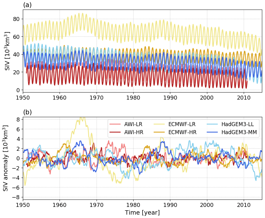
Figure 1 Sea ice volume time series from the six model configurations used in this work: (a) absolute values and (b) anomalies in which the long-term trends and the seasonal cycles were subtracted from the original time series.

2.2 Potential predictors

In this section, we identify potential predictor variables for use as input into the empirical statistical model that predicts SIV anomalies. Apart from the condition that all predictor variables could be regularly sampled from observational platforms in the real world, we only preselected variables which have the potential to impact the sea ice through dynamic and/or thermodynamic processes. Overall, two categories of predictors are tested: integrated variables, intrinsically represented by a single pan-Arctic time series, and predictors represented by several gridded time series of the same variable. Here, predictor variables are also considered in terms of their anomaly.

In total, a set of seven predictors are considered for this preliminary inspection. Three of them are integrated variables that are pan-Arctic SIV itself, pan-Arctic sea ice area (SIA), and Atlantic basin ocean heat transport (OHT) estimated at 60.0^∘ N. The other four predictors are variables organized in a gridded format and are sea ice thickness (SIT), sea ice concentration (SIC), sea surface temperature (SST), and sea ice drift (Drift). Figure 2 shows an example case (AWI-LR) in which the predictand (SIV) is compared with the two intrinsic pan-Arctic predictors (Fig. 2a, b) and with the four gridded predictors (Fig. 2c–j). As a first test, we inspect the performance of pan-Arctic predictors by estimating their lag-0 correlation against the predictand. The correlation coefficients shown in the second (SIA) and third (OHT) columns of Table 1 indicate that SIA is a valid predictor for all model outputs, while OHT is significantly correlated only for the low-resolution versions of the models.

Table 1 Lag-0 correlation coefficient estimated between the predictand (SIV anomaly) and a set of pan-Arctic potential predictors: SIA, OHT, SIT, SIC, SST, and Drift. The correlation coefficients between OHT and SIV anomaly for the high-resolution model versions are not shown since only statistically significant coefficients are displayed in the table. Regional predictors (SIT, SIC, SST, and Drift) are represented by pan-Arctic averages. As for the predictand, all predictors are used with monthly time resolution and in terms of their anomaly.

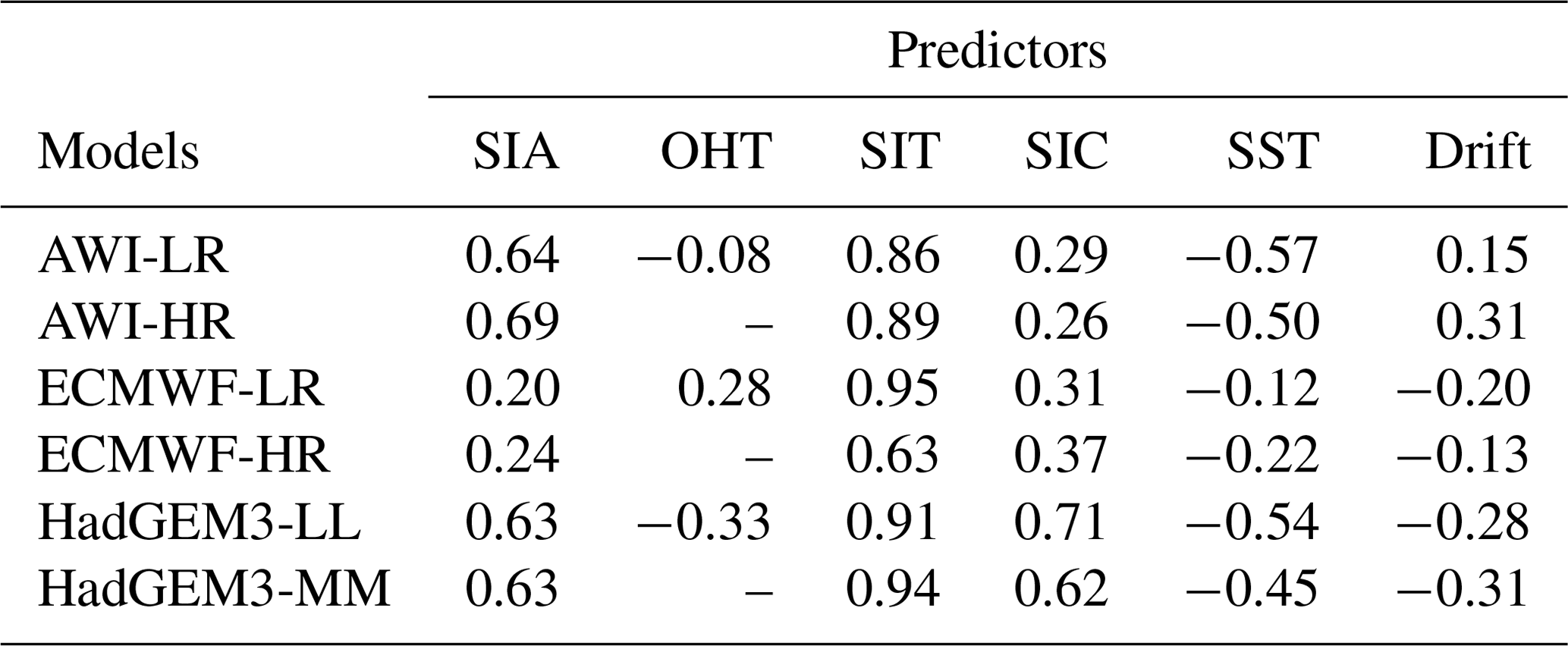
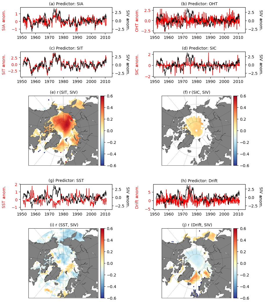
Figure 2 Lag-0 comparison between the time series from the predictand (SIV (10³ km³); black lines) and predictors: (a) SIA (10⁶ km²), (b) OHT (PW), (c) SIT (m), (d) SIC (%), (g) SST (^∘C), and (h) Drift (km d⁻¹) (red lines). The correlation maps used for normalizing the regional predictors, as suggested by Drobot et al. (2006), are also shown: (e) SIT, (f) SIC, (i) SST, and (j) Drift. Here, AWI-LR is merely used as an example case and not for a specific reason.

To obtain the same first assessment for the other predictors, the gridded values are reduced to their pan-Arctic average. To do so, the time series are normalized twice: first, by the grid area of each grid cell and, second, by the correlation maps with the predictand (Drobot et al., 2006), as shown in Fig. 2e, f, i, j. In the second normalization, the significant correlation coefficients from the different grid cells are used as normalizing factors (as is the grid cell area in the first normalization). The idea behind this second normalization is to take advantage of the correlations between predictand and predictors since the former is not necessarily correlated to the latter over the entire Arctic domain. Note in the maps that insignificant correlation coefficients are set to zero (white regions) so that they do not weigh in the normalization (Fig. 2e, f, i, j). The red lines in Fig. 2c, d, g, h show the respective SIT, SIC, SST, and Drift anomalies reduced to their pan-Arctic averages, which are in turn significantly correlated with the predictand in all model outputs (Table 1).

2.3 Statistical empirical models

The basis of our statistical empirical model (SEM) is a multiple linear regression model where the time series of the dependent variable (y) could be described as a function of the time series of the independent explanatory variables (x_i), as follows:

$$\begin{array}{}\text{(1)}& y={\mathit{\beta }}_{\mathrm{0}}+{\mathit{\beta }}_{\mathrm{1}}{x}_{\mathrm{1}}+{\mathit{\beta }}_{\mathrm{2}}{x}_{\mathrm{2}}+\mathrm{\dots }+{\mathit{\beta }}_k{x}_k,\end{array}$$

where β₀ is the constant y intercept, and β_k represents the slope coefficients for each explanatory variable of the empirical model.

In our case, the reconstructed time series of SIV anomaly (SIV_rec) is based on the linear relationship between this variable and the predictors mentioned in Sect. 2.2. If the SIV itself is also considered a predictor, the multiple linear regression in Eq. (1) can be written as

$$\begin{array}{}\text{(2)}& \begin{array}{rl}{\mathrm{SIV}}_{\mathrm{rec}}=& {\mathit{\beta }}_{\mathrm{0}}+{\mathit{\beta }}_{\mathrm{1}}\mathrm{SIV}+{\mathit{\beta }}_{\mathrm{2}}\mathrm{SIA}+{\mathit{\beta }}_{\mathrm{3}}\mathrm{OHT}+{\mathit{\beta }}_{\mathrm{4}}\mathrm{SIT}\\ & +{\mathit{\beta }}_{\mathrm{5}}\mathrm{SIC}+{\mathit{\beta }}_{\mathrm{6}}\mathrm{SST}+{\mathit{\beta }}_{\mathrm{7}}\mathrm{Drift}.\end{array}\end{array}$$

To ensure robustness to the statistical reconstructions, the SEM is applied within a Monte Carlo loop with 500 repetitions. In every repetition, 70 % of the data are randomly selected for training (N_T) the SEM, while the remaining 30 % are used for comparing (N_C) the original and the reconstructed SIV. In practical terms, ECMWF and HadGEM3 have 780 data points in time equivalent to the 780 months between January 1950 and December 2014 (720 for AWI; from January 1951 to December 2010) so that N_T=546 monthly values are used for building the SEM and N_C=234 values are used to evaluate how good the SIV reconstruction is (N_T=504 and N_C=216 for AWI). Since our main interest lies in the reconstruction of the SIV values, the metric used for comparing the original and reconstructed time series is the root-mean-squared error (RMSE). In this way, the score (Sc) of the reconstructed SIV can be represented by

$$\begin{array}{}\text{(3)}& \mathrm{Sc}={\displaystyle \frac{\mathrm{1}}{R}}\sum _{r=\mathrm{1}}^R\sqrt{{\displaystyle \frac{{\sum }_{n=\mathrm{1}}^{N_{\mathrm{C}}}\left({\mathrm{SIV}}_{\mathrm{rec}}\right(P)-\mathrm{SIV}{)}^{\mathrm{2}}}{N_{\mathrm{C}}}}},\end{array}$$

where R=500 indicates the number of interactions in the Monte Carlo loop, P represents the (set of) employed predictor(s), and the index N_C emphasizes that only 30 % of the data are used for comparison between original (SIV) and reconstructed SIV (SIV_rec) time series. An estimate of the Sc error (Sc_er) is given by the standard deviation calculated from the set of RMSEs given at every step of the Monte Carlo scheme.

Two different approaches for applying the SEM are used in this work. First, in Sect. 3.1, we evaluate the individual and combined performances of the pan-Arctic predictors (intrinsic and averaged ones; see Sect. 2.2) for reconstructing the SIV anomaly at different months of the year (March and September), with a lag of 1 to up to 12 months upfront. Here, SIV itself is also allowed as an individual predictor to test the auto-prediction ability of this variable from lagged months. However, we are aware that SIV as a predictor could dominate the results since autocorrelation is expected to be stronger compared to the correlation with other variables. Therefore, SIV itself will not be used as a predictor in combination with other variables as generically described in Eq. (2) (see further Figs. 4h and 5h). Second, in Sect. 3.2, we make use of the SEM to support an optimal sampling strategy, but using the predictors in their gridded format rather than their pan-Arctic averages, as the methodology described in Sect. 2.4. In this case, SIV itself is not used as a predictor at all.

2.4 Identifying optimal sampling locations

We intend to identify a reduced number of sites from which predictor variables could offer an optimal representation of the pan-Arctic SIV anomaly. To identify the first best location, a score map (Sc[i,j]) is created by applying the methodology described in Sect. 2.3 at each grid cell[i,j]. However not all grid point predictors (SIT[i,j], SIC[i,j], SST[i,j], Drift[i,j]) are necessarily used, only the valid ones. That means only predictors significantly correlated with the predictand are used. For instance, for the AWI-LR product, the SEM applied for a grid point placed off the eastern coast of Greenland will incorporate SIT, SST, and Drift as predictors while SIC is disregarded, as suggested by the correlation maps plotted in Fig. 2e, f, i, j. SIA is the only intrinsic pan-Arctic predictor kept at this stage. The motivation for using SIA as a predictor is justified by the fact that this variable is already provided year-round by satellites so that it could be combined with in situ parameters in a real monitoring programme. OHT is not used at this stage since it turned out that this predictor provides a relatively poor prediction to the predictand, as discussed further in Sect. 3.1. Also, from an observational point of view, sampling OHT is a very complex task that requires oceanographic observations well-distributed both horizontally and in depth. SIV is disregarded for an obvious reason since this is the variable that we supposedly do not have and want to predict.

By following the approach above, the goal is to create a first score map (Sc[i,j]) from which the first best location can be identified. In that Sc[i,j], the smaller the score, the better the grid point can reproduce the pan-Arctic SIV. The first best location is the one represented by the smallest score in the Sc[i,j]. Each of the six model outputs has its first score map. That means that each of the datasets provides its first optimal location (Sc[i₁,j₁]). In practical terms, the score maps will reveal not only a single best location, but also clusters of grid points defining one (or more) region(s) from where the SIV anomalies would be optimally reconstructed (see further in Sect. 3.2.1).

Aiming at spotting a single first optimal location that better represents all datasets (ensemble first optimal location), we take the average of the six score maps. To give the same weight for all datasets in the averaging, the individual score maps are scaled between zero and 1 (ScNorm_[i,j]; Calado et al., 2008), as follows (Eq. 4):

$$\begin{array}{}\text{(4)}& {\mathrm{ScNorm}}_{[i,j]}={\displaystyle \frac{{\mathrm{Sc}}_{[i,j]}-{\mathrm{Sc}}_{\min }}{{\mathrm{Sc}}_{\max }-{\mathrm{Sc}}_{\min }}},\end{array}$$

where the indexes min and max indicate the minimum and maximum values in the score map, respectively. Afterward, for having a coherent grid for averaging all normalized score maps, the six models are interpolated into a common $\mathrm{1}{}^{\circ }\times \mathrm{1}$^∘ grid. Besides the inherent different spatial grid resolution of the models, this step has no impact on the results since the best-performing regions in the score maps are preserved (not shown). Finally, the first best ensemble sampling location is defined as the geographical coordinate where the mean ScNorm map presents its minimum value. This approach has the advantage of reducing the model dependence of the results by relying on different datasets.

After determining and fixing the first ideal location [i₁,j₁], we search for a second [i₂,j₂], a third [i₃,j₃], and so on [i_k,j_k], best locations. However, every time that a new location is identified, a region surrounding this point is also defined in order to avoid that two optimal sites are placed in close proximity of each other. To do so, we follow the concept of length scale (Blanchard-Wrigglesworth and Bitz, 2014; Ponsoni et al., 2019). The length scale defines a radius where a certain gridded variable is well-correlated to the same variable from the neighbouring grid points. In this work we do not use a radius, but a very similar approach: the correlation coefficient of our best predictor at the selected location (SIT_[ik,jk]; see Sect. 3.1) is calculated against the equivalent time series from all the other grid points (SIT_[i,j]). The region defined by the grid points with a correlation higher than 1∕e, a threshold for correlations below which the SIT is assumed to be uncorrelated to the point of interest, is used as a restricting region. This region is hereafter defined as “region of influence”. So, all grid points enclosed in the region of influence are automatically disregarded from being selected as the next optimal location. As an example, the region of influence for a station arbitrarily placed at the North Pole, as defined by the ensemble of datasets, exhibits departures from concentric reflecting the transpolar drift (Fig. 3).

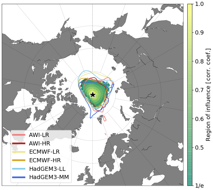
Figure 3 Region of influence for a station arbitrarily placed at the North Pole (black star) as defined by each model (colourful lines) and by the averaged region of influence from the different models (shades of green to yellow).

In this approach, the regression described in Eq. (2), with k optimal locations, takes the following format:

$$\begin{array}{}\text{(5)}& \begin{array}{rl}{\mathrm{SIV}}_{\mathrm{rec}}& ={\mathit{\beta }}_{\mathrm{0}}+{\mathit{\beta }}_{\mathrm{2}}\mathrm{SIA}+\sum {\mathit{\beta }}_{P_{\mathrm{1}}[i_{\mathrm{1}},j_{\mathrm{1}}]}{P}_{\mathrm{1}}[i_{\mathrm{1}},j_{\mathrm{1}}]\\ & +\sum {\mathit{\beta }}_{P_{\mathrm{2}}[i_{\mathrm{2}},j_{\mathrm{2}}]}{P}_{\mathrm{2}}[i_{\mathrm{2}},j_{\mathrm{2}}]+\mathrm{\dots }\\ & +\sum {\mathit{\beta }}_{P_k[i_k,j_k]}{P}_k[i_k,j_k],\end{array}\end{array}$$

where the term ${\mathit{\beta }}_{P_k[i_k,j_k]}{P}_k[i_k,j_k]$ represents the product between the valid predictors P_k[i_k,j_k], at the optimal location number k, and their respective slope coefficients ${\mathit{\beta }}_{P_k[i_k,j_k]}$. It is worth mentioning that only valid predictors, which means only predictors from grid points placed outside the region of influence defined by previously selected points and that are validated by the correlation map criterion, are used in Eq. (5).

3 Results

3.1 Statistical predictability of SIV anomaly: pan-Arctic predictors

In this section, the statistical predictability of the SIV anomaly is quantitatively evaluated by considering leading periods of 1 to 12 months. Also, the predictive performance of seven pan-Arctic predictors is tested. The predictors are SIV itself, SIA, OHT, SIT, SIC, SST, and Drift. Here, we focus on the months with relatively large (March; Sect. 3.1.1) and reduced (September; Sect. 3.1.2) SIV at the end of the winter and summer, respectively.

3.1.1 Statistical predictability of March SIV anomaly: pan-Arctic predictors

Figure 4 displays the predictive performance (quantified by the RMSE) of different predictors for estimating March SIV anomalies. The SIV itself is the best predictor variable and its score gradually increases from 12 (Sc = 1.0 ×10³ km³) to four (Sc = 0.68 ×10³ km³) leading months. During this period the mean performance for the ensemble of models increases by about 32 %. As per 3 leading months, from December to February, the predictive capability substantially improves by 43 % (Sc = 0.57 ×10³ km³), 59 % (Sc = 0.41 ×10³ km³), and 77 % (Sc = 0.23 ×10³ km³), respectively (Fig. 4a). The second best predictor is the SIT, which has performance similar to the SIV predictor from about 12 to 9 leading months (ensemble mean Sc = 1.02 ×10³ km³, 1.03 ×10³ km³, 1.0 ×10³ km³; Fig. 4d). Nevertheless, its score remains relatively stable and improves only by about 25 %, from May to February (Sc = 1.0 and 0.75 ×10³ km³). SIC (Fig. 4e), SST (Fig. 4f), and Drift (Fig. 4g) have poorer performance compared to SIT but similar behaviour, with the score slightly improving over time until one leading month. SIA (Fig. 4b) is a valid predictor for the AWI and HadGEM3 models, but it does not seem to be the case for ECMWF versions. Finally, OHT was shown to be a poor predictor in terms of monthly predictability. For most of the leading months and models, the statistical reconstruction is not significant when estimated with this predictor (Fig. 4c).

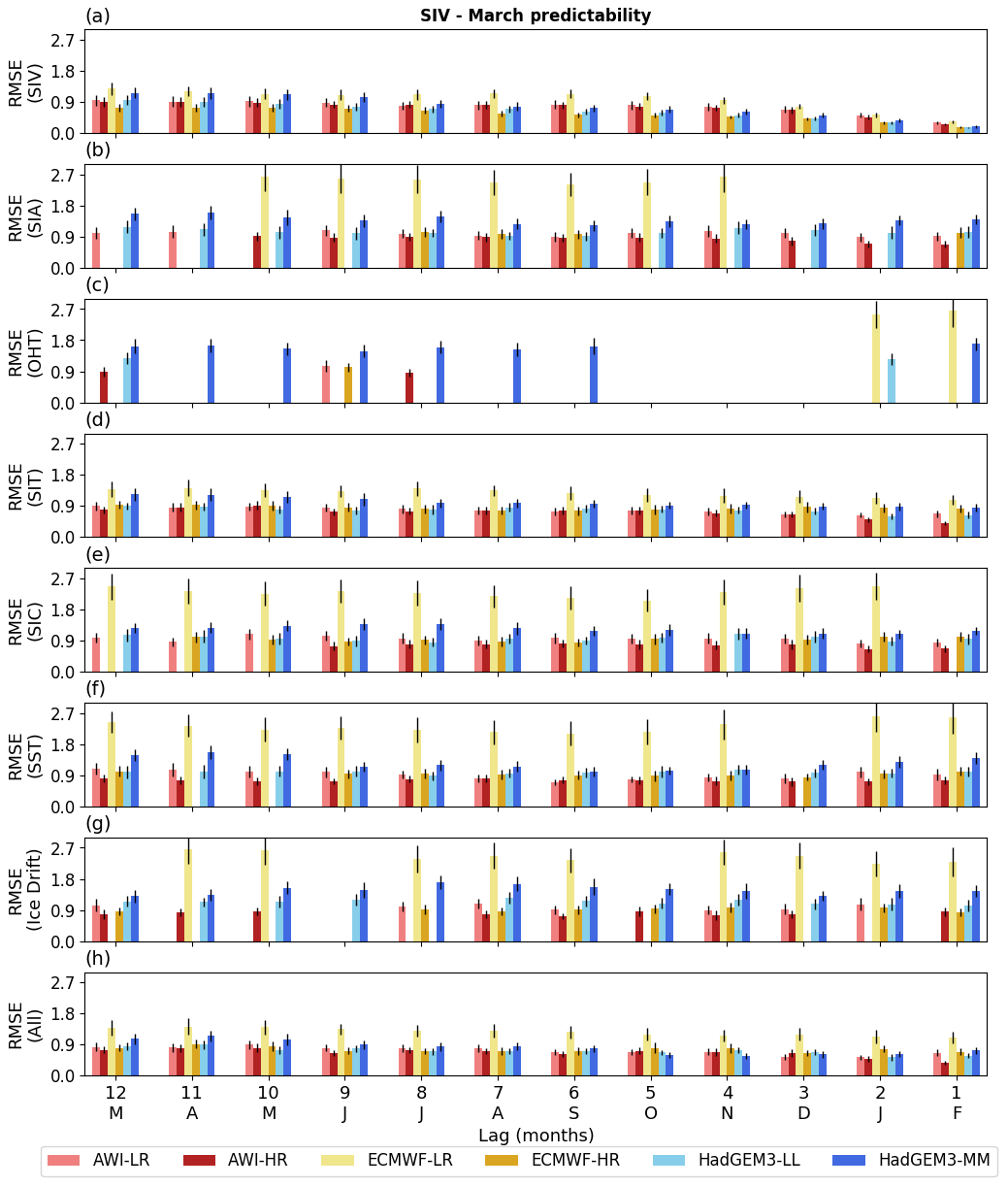
Figure 4 Statistical predictability of the March SIV anomalies, estimated from 12 leading months and quantified by the RMSE (10³ km³) calculated between the original and reconstructed time series (Sc), as prescribed by seven predictors: (a) SIV itself, (b) SIA, (c) OHT, (d) SIT, (e) SIC, (f) SST, (g) Drift. The predictions employing all predictor variables (except the SIV itself) are displayed in (h). The vertical black lines indicate the error as provided by the 500 Monte Carlo simulations. The statistical predictability follows the methodology introduced in Sect. 2.3. Missing vertical bars mean that the statistical reconstruction is not statistically significant. The long-term trend and seasonal cycle are excluded from both predictand and predictors.

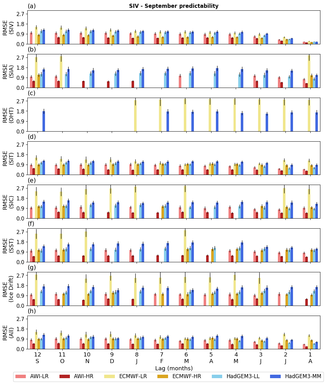
Figure 5 Statistical predictability of the September SIV anomalies, estimated from 12 leading months and quantified by the RMSE (10³ km³) calculated between the original and reconstructed time series (Sc), as prescribed by seven predictors: (a) SIV itself, (b) SIA, (c) OHT, (d) SIT, (e) SIC, (f) SST, (g) Drift. The predictions employing all predictor variables (except the SIV itself) are displayed in (h). The vertical black lines indicate the error as provided by the 500 Monte Carlo simulations. The statistical predictability follows the methodology introduced in Sect. 2.3. Missing vertical bars mean that the statistical reconstruction is not statistically significant. The long-term trend and seasonal cycle are excluded from both predictand and predictors.

A way of further improving the statistical predictability is to use several predictors at once. Figure 4h shows the case where all the aforementioned predictors (except SIV) are used by the empirical model. For this configuration, the predictive skill is still 10 % lower than the case where SIV is standing alone as a predictor, but it is about 10 % better than the reconstructions provided only by the SIT. The inter-model comparison does not show a conclusive answer to the question of whether or not the model resolution plays a role in the statistical predictability of March SIV anomalies. Overall, AWI-HR predictors are more skilled than AWI-LR predictors, though the opposite is observed for HadGEM3. For the ECMWF versions, the SIV anomalies from ECMWF-HR present better reproducibility, while ECMWF-LR presents much larger errors. Note that ECMWF-LR has a mean state characterized by a much thicker sea ice and, consequently, higher variance (see Fig. 1). This is the reason that makes ECMWF-LR an outlier compared to the other five model outputs for this and other results found in this paper (see further discussion in Sect. 4).

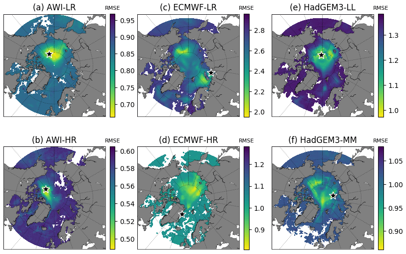
Figure 6 Score maps (Sc[i,j]) represented by the RMSE (10³ km³) calculated at every grid cell between the original and the reconstructed SIV anomalies. The smaller the RMSE (shades of yellow), the higher the performance of the grid point for reconstructing the SIV anomaly. The black star indicates the primary optimal location for each model Sc[i1,j1]. Note that the colour map scale is different for each map.

3.1.2 Statistical predictability of September SIV anomaly: pan-Arctic predictors

A similar scenario compared to March is found for the September SIV anomaly predictability (Fig. 5). The best predictor is the SIV itself (Fig. 5a) for which the predictive skill improves by about 83.6 % from the previous September to August (Sc = 1.16 ×10³ and 0.19 ×10³ km³). This improvement is mainly attributed to the 3 months before September: Sc = 0.71 ×10³, 0.44 ×10³, and 0.19 ×10³ km³ for June, July, and August, respectively. The second best predictor is SIT (Fig. 5d), while SIC (Fig. 5e), SST (Fig. 5f), and Drift (Fig. 5g) present an intermediate performance. For the former four predictors, the ensemble mean Sc slightly improves from 12 to 1 leading months in about 28.8 % (Sc = 1.04 ×10³ and 0.74 ×10³ km³), 15 % (Sc = 1.40 ×10³ and 1.19 ×10³ km³), 29 % (Sc = 1.26 ×10³ and 0.90 ×10³ km³), and 24 % (Sc = 1.46 ×10³ and 1.11 ×10³ km³), respectively. Not all tested predictors are statistically significant for reproducing the SIV anomalies. Again, this is the case for OHT (Fig. 5c). SIA also presents poor performance for some models and leading months (Fig. 5b). Another resemblance to March predictability is the relatively poor performance presented by the predictor variables from ECMWF-LR.

3.2 Statistical predictability of SIV anomaly: regional predictors

In this section, the empirical statistical model is used for supporting an optimal sampling strategy by following the methodology described in Sect. 2.4. To do so, we evaluate the predictors at every grid point rather than use their pan-Arctic averages. The reasoning behind this approach lies in the hypothesis that the statistical empirical model can fairly reproduce and/or predict the SIV anomalies if a few optimal locations provide in situ measurements from the predictor variables. These in situ observations can be applied concomitantly with predictors that are continuously measured by satellites such as the pan-Arctic SIA and the SIC.

Here we assume that numerical models are able to reproduce the main physical processes behind the interactions among predictand and predictors. Practically, we will take into account four gridded predictors, SIT, SIC, SST, and Drift, and one pan-Arctic predictor SIA, although it is worth reminding ourselves that only predictors significantly correlated with the predictand will be incorporated into the statistical model. As per the results of Sect. 3.1, the OHT will not be included as a predictor variable due to its poor capability to provide a skilful prediction, being reinforced by the difficulties associated with the in situ sampling and estimation of this variable.

3.2.1 Optimal sampling locations

For each of the six model realizations, score maps (Sc[i,j]; Eq. 3) were determined with the aim of spotting the location that can better reproduce the SIV anomalies as shown in Fig. 6. This location is thus defined as the grid point with minimum RMSE calculated between the original and reconstructed time series (Sc[i1,j1]; black stars in Fig. 6). The resulting ideal locations for AWI-LR, AWI-HR, and HadGEM-LL (Fig. 6a, b, e) are relatively close to each other, separated by a maximum of ∼ 600 km. Even though ECMWF-LR, ECMWF-HR, and HadGEM3-MM (Fig. 6c, d, f) suggest optimal locations that are placed farther from the sites suggested by the other datasets, their score maps still suggest a relatively good skill (low RMSE values) at the common region occupied by the three previous referred models. This fact further justifies the multi-model approach used in this work.

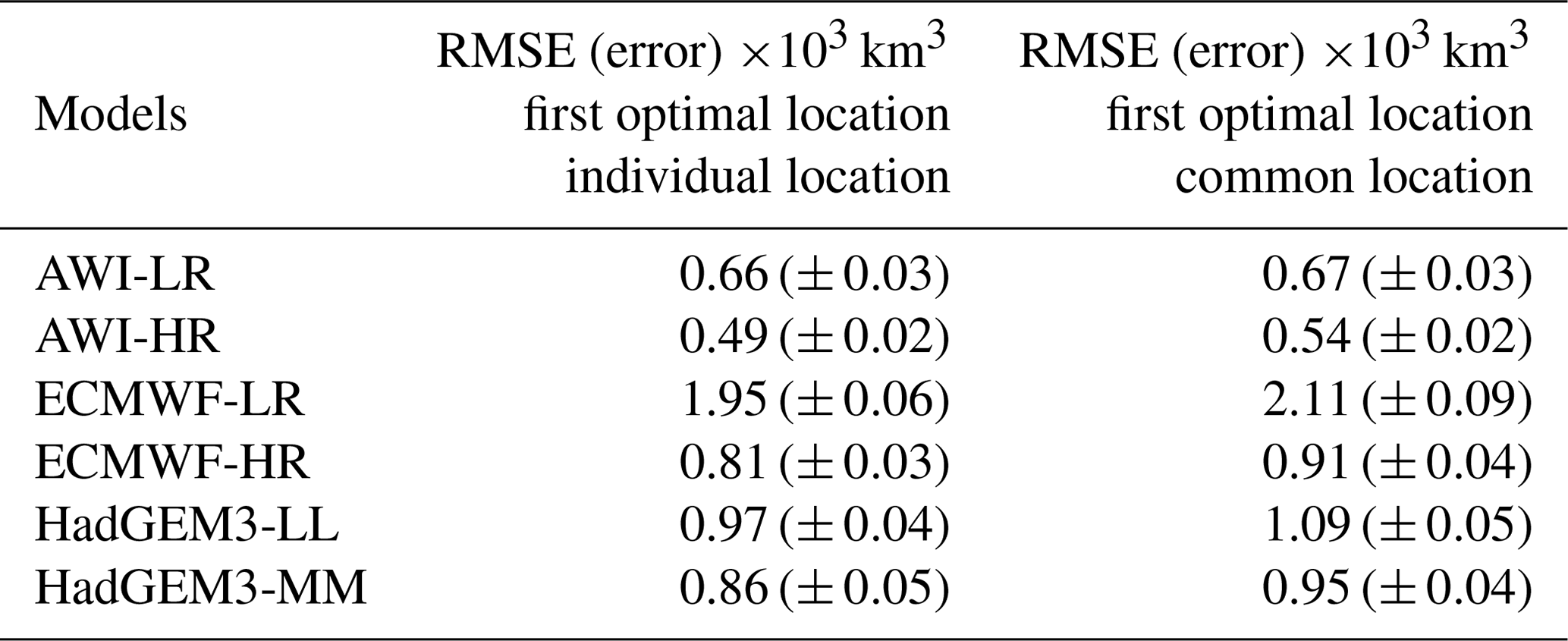
The RMSEs (and associated SD from the Monte Carlo scheme) calculated between the original SIV anomalies and the SIV anomalies reconstructed by the SEM, using predictor variables from the first optimal location (black stars in Fig. 6), are shown in the middle column of Table 2. Based on those values, predictor variables from the AWI systems can better reproduce the SIV anomalies compared to the predictors from HadGEM and ECMWF. For the three models, the high-resolution version provides better statistical predictability. A common score map, with the indication of a common first optimal location placed at the transition Chukchi Sea–central Arctic–Beaufort Sea (79.5^∘ N, 158.0^∘ W), is shown in Fig. 7a. This common location is found through the ensemble mean of the scaled individual score maps, following the methodology described in Sect. 2.4. The RMSE values from that common location (Fig. 7a), but retrieved from the score maps in Fig. 6, are shown in the right column of Table 2. The predictive skill drops by about 10 % when the common point is chosen for all models, except for AWI-LR which presents similar results for the two locations. These values reinforce that, at least for this first location, the predictors from the high-resolution outputs lead to a better predictive skill compared to the low-resolution predictors from their counterpart. Note that this was not the case when using pan-Arctic predictors in Sect. 3.1.

Table 2 Mean RMSEs (and associated SDs, error) from the 500 Monte Carlo realizations calculated between the original SIV anomalies and the SIV anomalies reconstructed by the SEM. We recall that in each Monte Carlo realization 70 % of the data are randomly used for training the SEM, while 30 % are used for calculating the error. The middle column shows the values for the case where the predictors are extracted from the individual optimal locations, while the right column shows the values found with predictors from the common optimal location.

Once the primary common optimal site has been identified and accepted for all datasets, we search for the second best location. For that, the neighbouring grid points which fell into the region of influence of the first best site are not considered as a second option. Figure 7b shows the first location's region of influence. The procedure followed for identifying the first and second sites is thus repeated for the nth next locations. Aiming at improving the reconstruction of the SIV anomalies, every time that a new location is set, the valid predictors from this new point add to the predictors from the previous stations into the SEM. Figure 7c, e, g, i show the second to the fifth optimal sites accompanied by their respective regions of influence (Fig. 7d, f, h, j). The second site is about 167 km from the North Pole. The third, fourth, and fifth points are placed at the offshore domain of the Laptev Sea near the transition with the central Arctic, in the central Arctic to the north of the Canadian Islands, and within the Beaufort Sea, respectively.

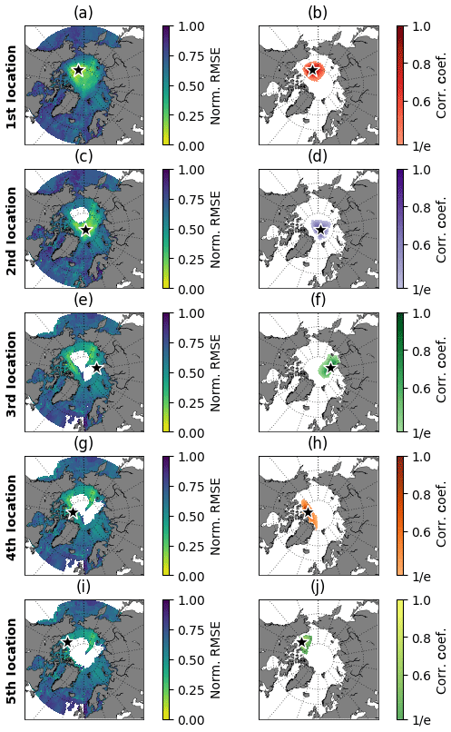
Figure 7 (a) Ensemble mean–normalized score map (ScNorm) for the first best sampling location. (b) The region of influence is defined for the first best location. The panels (c, d), (e, f), (g, h), and (i, j) represent the same as (a, b) but for the second, third, fourth, and fifth best sampling locations, respectively.

Figure 8 represents an idealized scenario with the 10 best locations and their respective regions of influence. In such a context, the selection of points respects the hierarchy of the regions of influence in a way that the second site can not be placed within the region of influence no. 1 (shades of red), the third point can not be placed within the regions of influence nos. 1 and 2 (shades of red and purple), and so on. Note that with the proposed methodology, the regions of influence from the first 10 locations cover almost the entire Arctic Ocean and adjacent seas, with the exception of the Canadian Archipelago, the Kara Sea, and the Greenland Sea (see Fig. 9). But even for the two later cases, the region of influence from other locations partially covers these seas (Fig. 9; black line). The question of whether or not all 10 locations are indeed required to fairly predict the SIV anomalies, in terms of both anomaly values and variability, will be answered in the next sections.

Table 3 displays the geographical coordinates of the 10 locations as well as the Arctic subregions occupied by them, as identified in Fig. 9. The division of the Arctic into subregions is based on the classical definition adopted by the broadly used Multisensor Analyzed Sea Ice Extent – Northern Hemisphere (MASIE-NH) product, which is made available by the National Snow and Ice Data Center (NSIDC). Most of the stations are placed within the central Arctic (second, fourth, and eighth) or, as mentioned above, in the transition of this region with the Chukchi Sea (first) and Laptev Sea (third), where the sea ice tends to be perennial. The fifth location is placed at the central part of the Beaufort Sea. The sixth and ninth stations are located at the offshore and inshore limits of the East Siberian Sea, respectively. The seventh site is suggested to be at the Barents Sea off Severny Island, and the 10th station occupies the near-coastal Laptev Sea.

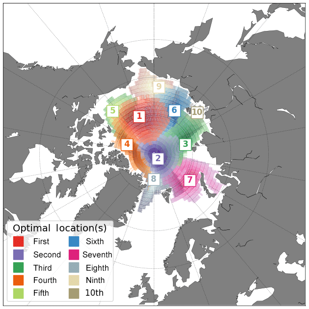
Figure 8 Optimal observing framework, as suggested by the ensemble of model outputs, for sampling predictor variables in order to statistically reconstruct and/or predict the pan-Arctic SIV anomaly. The numbers indicate the first up to the 10th best observing locations in respective order. The hatched area around each location (same colour code) represents their respective region of influence. The selection of points respects the hierarchy of the regions of influence in a way that the second point can not be placed within the region of influence no. 1 (shades of red), the third point can not be placed within the regions of influence nos. 1 and 2 (shades of red and purple), and so on.

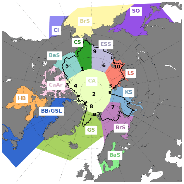
Figure 9 Optimal observing framework for sampling predictor variables in order to statistically reconstruct and/or predict the pan-Arctic SIV anomaly. The numbers indicate the first up to the 10th optimal sites. Each of the coloured areas represents an Arctic subregion according to the Arctic subdivision suggested by the National Snow and Ice Data Center (NSIDC). The black line indicates the global region of influence defined in Fig. 8 (colour-shaded areas). Abbreviations: Beaufort Sea (BeS); Chukchi Sea (CS); East Siberian Sea (ESS); Laptev Sea (LS); Kara Sea (KS); Barents Sea (BrS); Greenland Sea (GS); Baffin Bay/Gulf of St. Lawrence (BeS); Canadian Archipelago (CaAr); Hudson Bay (HB); central Arctic (CA); Bering Sea (BrS); Baltic Sea (BaS); Sea of Okhotsk (SO); Cook Inlet (CI).

Table 3 Geographical coordinates for the first 10 optimal sampling locations (second and third columns). The fourth column shows the subregions in which each of the points is placed in (see Fig. 9). The limits of the subregions are suggested by the National Snow and Ice Data Center (NSIDC).

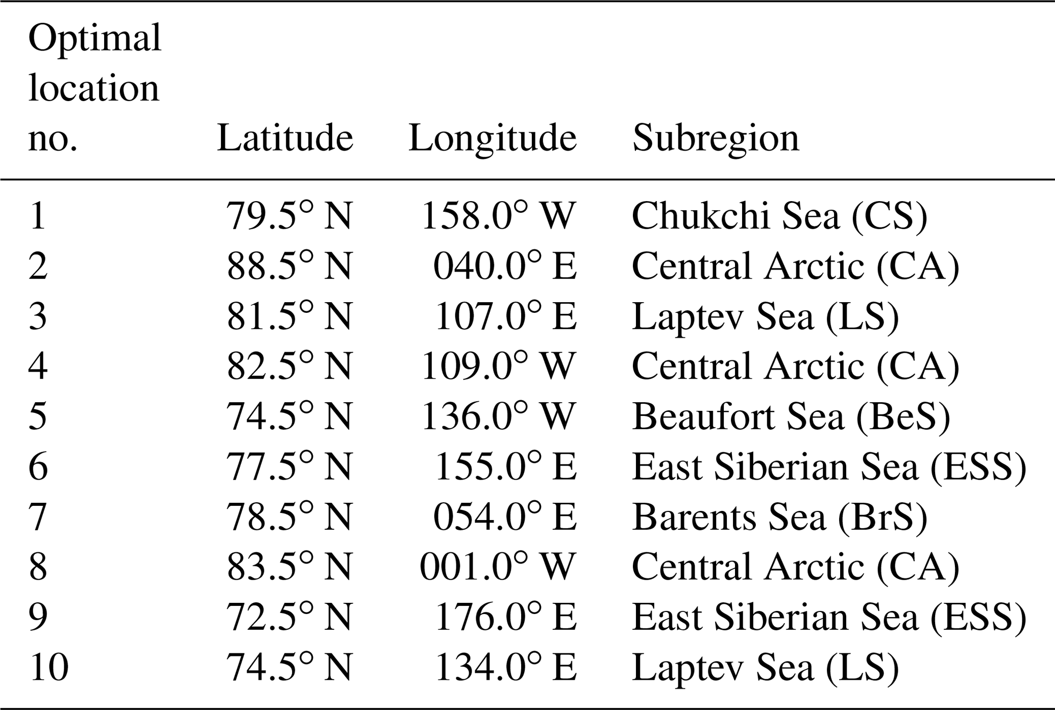
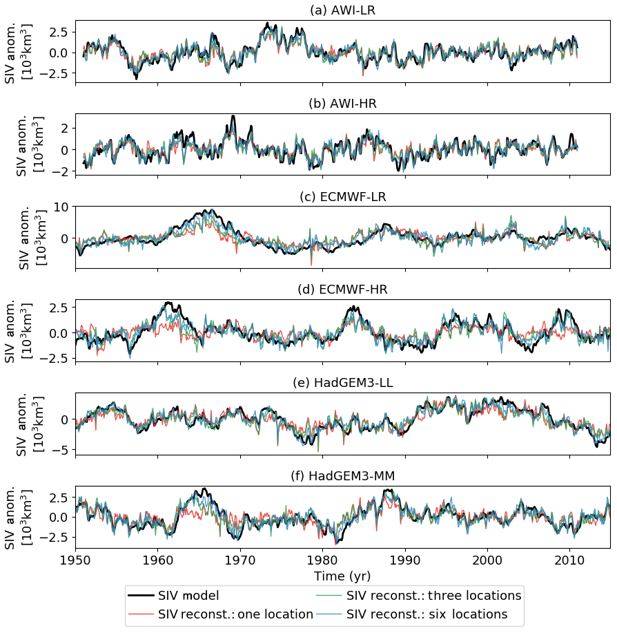
Figure 10 Lag-0 comparison between the original (black) and statistically reconstructed SIV anomalies. The reconstruction takes into account the first (red), the three first (first–third; green), and the six first (first–sixth; blue) optimal locations: (a) AWI-LR, (b) AWI-HR, (c) ECMWF-LR, (d) ECMWF-HR, (e) HadGEM-LL, and (f) HadGEM-MM. Note the different scales on the y axes.

3.2.2 Reconstructed SIV anomaly

Once the ideal sampling locations are established, these sites are used to effectively reconstruct the entire time series of SIV anomalies from the six model outputs, by taking into account only the valid predictors from each location. We will make use of the RMSE to evaluate how good our statistical prediction is in terms of absolute values as in the previous sections, but here we are also interested in inspecting the ability of the empirical model to reproduce the full variability of the SIV anomalies. For that, apart from the RMSE, we also calculate the coefficient of determination (R²) between the original and reconstructed time series.

Figure 11 (a) RMSE (y axis) estimated between the original and reconstructed time series by taking into account predictor variables from one up to 10 optimally selected locations (x axis). (b) Same as (a) but using R² (y axis) to compare original and reconstructed time series. (c) Valid predictors, as determined by the correlation maps, retrieved from each targeted location. If a predictor is valid (y axis), its respective symbol, as defined in the inset legend from (b), is plotted. A black cross indicates that the predictor is not valid at the respective location.

Figure 10 provides a comparison at lag-0 between the original (black lines) and the reconstructed times series by taking into account the first (red lines), the three first (green lines), and the six first (blue lines) locations. For the first reconstruction, RMSE values are almost identical to the ones shown in the second column of Table 2 (see Fig. 11a; y axis = 1). Again, for all three models, the predictor variables from the higher-resolution versions present better performance in reproducing the SIV anomaly values. The relatively poor skill of the ECMWF-LR predictors compared to the other five systems is remarkable (Fig. 10c).

Figure 11a summarizes the RMSE values for the reconstructions conducted with data from only the first up to all 10 combined locations. The pattern of better prediction skill for the models with higher grid resolution revealed by the first location remains when more sites are incorporated into the SEM. From the ensemble means the RMSE (×10³ km³) values are, respectively, 1.06, 0.95, 0.90, 0.81, 0.78, 0.70, 0.65, 0.63, 0.60, and 0.59 for the reconstruction with one to 10 locations (black curve/points in Fig. 11a). By excluding the outliers from ECMWF-LR, the previous RMSEs decrease to about 20 % (as shown by the grey curve points in Fig. 11a). For most of the datasets, the statistical reconstruction seems to improve better until the incorporation of the fifth to sixth locations. As per the seventh location, the improvement seems to attenuate (Fig. 11a).

Figure 11b introduces a similar analysis but quantified by the R². Interestingly, for this metric, the ECMWF-LR is not outstanding from the others, and its predictors present a similar performance for reproducing the SIV anomaly variability. By account of the reconstructions with one to 10 optimal sites, the ensemble means of R² values are 0.53, 0.63, 0.67, 0.73, 0.75, 0.80, 0.81, 0.83, 0.84, and 0.84, respectively. These ensemble means suggest that the statistical empirical model could reproduce more than 60 % of the SIV variability by using predictors from only the first two optimal locations. AWI and HadGEM datasets indicate that four locations are sufficient for reproducing more than 70 % of the variability. With six well-positioned sites, about 80 % of the SIV anomaly may be explained as suggested by the ensemble mean (Fig. 11b). As per the sixth station, the gain from adding new locations seems to be minimal (∼ 1 %). In addition, it is of interest that the R² metric behaves in opposition to the RMSE since the best performing predictors are the ones coming from the model's version with lower grid resolution.

In terms of used predictor variables, Fig. 11c reiterates that SIT is the most skilful of the predictors. From the 60 cases that the SEM was applied to (six datasets, 10 locations), SIT was used 59 times. SIT was not a valid predictor only for the ninth location in ECMWF-HR. SST and Drift were used in about two-thirds of the cases (40 and 38 times, respectively), while SIC was used only in half (29 times) of the cases. Inspecting the individual model outputs, HadGEM (the two resolutions comprised) is the one in which the empirical model takes the best advantage of the available gridded predictors, having neglected one of them in only 15 out of 80 cases, while ECMWF and AWI have ignored predictors in 29 and 30 out of 80 cases, respectively.

To evaluate the performance and robustness of our SEM, the RMSE and R² calculated between the original and our-methodology-based reconstructed SIV anomalies (Fig. 11a, b) are compared against the same two metrics but now estimated by a simple multiple linear regression model having as input predictor data from random chosen locations (Fig. 12). For that purpose, 100 combinations of 10 randomly chosen locations were determined. For each combination, the SIV anomaly is reconstructed with predictor data from the first location, the first–second, the first–third, …, the first–10th locations. We have used the same predictor variables from randomly locations placed only into the global region of influence represented by the black line in Fig. 9. The results show that the SIV reconstructions based on our methodology (and optimally selected locations) are more skilful in terms of both RMSE and R². This is valid for all models, considering a single location or any combination of up to 10 locations (Fig. 12).

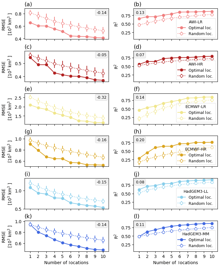
Figure 12 Root-mean-squared error (RMSE; left column) and coefficient of determination (R²; right column) calculated between the original and reconstructed SIV anomalies. The reconstructed SIV volume anomalies are based on the optimally selected locations following our methodology (full dots; same as in Fig. 11a, b), as well as by randomly chosen locations (empty dots). In the last case, 100 sets of 10 randomly chosen locations are used. For each of the 100 sets, the SIV anomaly is reconstructed using data from the first, the first–second, the first–third, …, the first–10th locations. The random locations are all enclosed in the global region of influence defined (Fig. 9; black line). The vertical bars associated with the empty dots represent the 1 standard deviation from the 100 reconstructions. The inset numbers represent the average difference between the two curves shown in each sub-panel.

4 Discussion

In this work, we have introduced a statistical empirical model for predicting the Arctic SIV anomaly on the interannual timescale. The model was built and tested with data from three AOGCMs (AWI-CM, ECMWF-IFS, and HadGEM3-GC3.1), each of which provided two horizontal resolutions, performing a total of six datasets. We have first inspected the predictive skill of seven different pan-Arctic predictors, namely SIV, SIA, OHT, SIT, SIC, SST, and Drift. These predictors were tested since they have dynamical and/or thermodynamical influence on the SIV. The three first predictors are intrinsically represented by single time series, while the remaining predictors are gridded variables that were reduced to mean pan-Arctic time series. From this first assessment, performed for the months of March and September, the results (Sect. 3.1) show that the best predictors are the SIV itself and the SIT, whilst SST, Drift, SIC, and SIA provide some intermediate-skill predictions. In general, such results are valid for predictions performed from 1 back to 12 leading months. For the SIV predictor, the skill substantially increases in the last 3 leading months. For the remaining aforementioned predictors, the skill slightly improves from 12 to 1 leading month.

In contrast, OHT provided very poor predictive skill. Docquier et al. (2019) recently showed (their Fig. 12) a relatively good correlation between OHT and the SIV. However, these authors correlated annual averages of OHT with monthly values of SIV, but here we are considering monthly means for all predictors. Based on that, the results from both papers suggest that the OHT has a cumulative impact on the sea ice throughout the year, which is not so remarkable when looking at individual months, even if several leading months are considered. One might wonder how SST is a relatively skilful predictor while OHT is not. We reiterate that the OHT tested as a predictor in this study is a remote parameter, which takes into account the seawater temperature (and meridional velocities) throughout the entire water column, calculated at 60.0^∘ N for the Atlantic basin ocean (Docquier et al., 2019). There are other potential candidates to explain why OHT is a poor predictor, for instance model biases such as an overestimation of the stratification at the near-surface layer, which could attenuate the heat content being transported towards the Arctic Ocean. Nevertheless, this is a subject that requires a more detailed investigation. From the results in Sect. 3.1 it is also noticeable that the ECMWF-LR predictors present a relatively poor skill compared to the others. This is explained by the fact that this model has a mean state characterized by a much thicker sea ice (see Fig. 1), impacting the RMSE used as a metric for evaluating the prediction skill.

We now recall and objectively answer the first open question posed in the introduction of this paper.

• i.

  What is the performance of different pan-Arctic predictors for predicting pan-Arctic SIV anomalies?
  Taking into account the ensemble mean, and using the average RMSE calculated between original and reconstructed SIV time series (Sect. 3.1; Figs. 4 and 5) for the last 3 leading months as score, the best predictors for March are sorted in the following order: SIV (0.41 ×10³ km³), SIT (0.78 ×10³ km³), SIA (1.01 ×10³ km³), SIC (1.10 ×10³ km³), SST (1.15 ×10³ km³), Drift (1.32 ×10³ km³), and OHT (2.05 ×10³ km³). The best predictors for September are sorted as SIV (0.45 ×10³ km³), SIT (0.76 ×10³ km³), SST (0.96 ×10³ km³), SIA (1.07 ×10³ km³), SIC (1.12 ×10³ km³), Drift (1.22 ×10³ km³), and OHT (2.24 ×10³ km³). If all predictors are used (except SIV itself), the averaged scores for 3 leading months are 0.70 ×10³ km³ for both March and September.

Once the statistical empirical model had been developed and the potential predictor variables are identified, we can make use of this information for recommending an optimal observing system. For example, such a system could be part of an operational oceanography programme in which predictor data are provided to the statistical model through in situ observations (e.g. oceanographic moorings and/or buoys) of SIT, SST, and Drift. The SIC and pan-Arctic SIA could also be incorporated into the statistical model since they are regularly sampled by satellites. OHT and the SIV are disregarded as predictors. The former is not a skilful predictor (as shown in Sect. 3.1), while the latter is the variable that we want to predict. We restricted our analyses to a maximum of 10 optimal locations, although a reduced number of observational sites are sufficient to fairly reproduce the SIV anomaly. The results from Sect. 3.2 provide further elements to answer the other three open questions of this study, as follows.

• ii.

  What are the best locations for in situ sampling of predictor variables to optimize the statistical predictability of SIV anomalies in terms of reproducibility and variability?
  The first 10 best sampling locations were identified. The exact coordinates of these locations are provided in Table 3 and also plotted in Figs. 8 and 9. As suggested by the ensemble of model outputs, the first optimal location is placed at the transition Chukchi Sea–central Arctic–Beaufort Sea (79.5^∘ N, 158.0^∘ W). The second, third, and fourth best locations are placed near the North Pole (88.5^∘ N, 40.0^∘ E), at the transition central Arctic–Laptev Sea (81.5^∘ N, 107.0^∘ E), and offshore of the Canadian Archipelago (82.5^∘ N, 109.0^∘ W).

• iii.

  How many optimal sites are needed for explaining a substantial amount (e.g. 70 % – an arbitrarily chosen threshold) of the original SIV anomaly variance?
  By considering an arbitrary threshold of 70 %, the systems AWI-LR (75 %), AWI-HR (73 %), HadGEM3-LL (79 %), and HadGEM3-MM (74 %) suggest that as few as four stations are sufficient to pass this threshold, which is also confirmed by the ensemble mean (73 %). Even though the ECMWF predictors have slightly low skill, they are still not far from the threshold: ECMWF-LR (66 %) and ECMWF-HR (64 %). The ensemble mean indicates that five and six well-placed stations could explain about 75 % and 80 % of the SIV anomaly variance, respectively. Adding further to six well-placed locations does not substantially improve the statistical predictability. A total of 10 locations explain about 84 % of the variance. However, as suggested by Fig. 8, even though the SEM seems to fairly reproduce the SIV anomaly variance and, therefore, the long-term variability, it found more difficulties to reproduce the short-term variabilities.

• iv.

  Are the results model dependent, in particular, and/or are they sensitive to horizontal resolution?
  The results suggest that statistical predictability is affected by model resolution. Notwithstanding, the question of whether or not a higher horizontal resolution provides better statistical predictability depends on the metric used to evaluate the predictions (Sect. 3.2.2 and Fig. 11). That is the case for RMSE, where the main target is to evaluate the reproducibility of the reconstructed values. It seems that an improved horizontal resolution allows a better trained statistical model so that the reconstructed values better approach the original SIV anomaly (Fig. 11a). On the other hand, investigating the interannual variability, the predictors provided by the numerical models with lower resolution are more able to match the reconstructed time series to the original SIV anomaly (Fig. 11b). As argued above, this study shows that model-based statistical predictability of SIV anomaly is sensible to the model horizontal resolution. Further investigation is needed to better understand the impact of model resolution on the SIV predictability.

5 Conclusions

We believe that this work positively impacts three aspects of a real-world observing system. First, it provides recommendations for optimal sampling locations. We are confident that our multi-model approach provides a solid view of the sites that better represent the variability of the pan-Arctic SIV. Second, even if those regions are not taken into account for any reason (for instance logistics, environmental harshness, strategical sampling, etc.), observationalists could still take advantage of the “region of influence” concept. By doing so, they avoid deploying two or more observational platforms that would provide relatively similar information in terms of pan-Arctic SIV variability. Third, considering that observational platforms are already operational, our SEM could be trained with model outputs (with the same or other state-of-the-art AOGCMs) and so incorporates observational data to project future pan-Arctic SIV variability. Within this context, we expect that this paper will provide recommendations for the ongoing and upcoming initiatives towards an Arctic optimal observing design.

Despite these promising results, we recognize that it might be harder to achieve skilful predictions in the real world employing statistical tools because the actual SIV variability is likely noisier than the one described by AOGCM outputs. While model results provide an average representation of variables inside a grid cell, real-world observations would be much more heterogeneous. This issue is even more pronounced when looking at our main predictor (SIT) due to the inherent roughness and short-scale spatial heterogeneity of the real-world SIT. As a consequence, this heterogeneity may be a source of uncertainties in a real observing system, and more observations would be required for effectively predicting the SIV anomaly. Some caution should be exercised since our findings might be slightly different for other AOGCMs. A good perspective for addressing this issue is to reapply the methodology developed in this paper, but using all models that will be made available through the CMIP6. Also, with the sea ice depletion, some of the suggested optimal sampling locations might in the future be ice free.

Finally, it is worth mentioning the recent effort from the scientific community to enhance the Arctic observational system. This effort takes place through recent observational programmes such as the Year of Polar Prediction (YOPP) (Jung et al., 2016) and the Multidisciplinary drifting Observatory for the Study of Arctic Climate (MOSAiC; https://www.mosaic-expedition.org/; last access: 1 March 2020).