the Creative Commons Attribution 4.0 License.
the Creative Commons Attribution 4.0 License.
 | 23 Jul 2020
The Arctic Ocean Observation Operator for 6.9 GHz (ARC3O) – Part 2: Development and evaluation
Clara Burgard
Dirk Notz
Leif T. Pedersen
Rasmus T. Tonboe
The observational uncertainty in sea ice concentration estimates from remotely sensed passive microwave brightness temperatures is a challenge for reliable climate model evaluation and initialization. To address this challenge, we introduce a new tool: the Arctic Ocean Observation Operator (ARC3O). ARC3O allows us to simulate brightness temperatures at 6.9 GHz at vertical polarization from standard output of an Earth System Model. To evaluate sources of uncertainties when applying ARC3O, we compare brightness temperatures simulated by applying ARC3O on three assimilation runs of the MPI Earth System Model (MPI-ESM), assimilated with three different sea ice concentration products, with brightness temperatures measured by the Advanced Microwave Scanning Radiometer Earth Observing System (AMSR-E) from space. We find that the simulated and observed brightness temperatures differ up to 10 K in the period between October and June, depending on the region and the assimilation run. We show that these discrepancies between simulated and observed brightness temperature can be attributed mainly to the underlying observational uncertainty in sea ice concentration and, to a lesser extent, to the data assimilation process, rather than to biases in ARC3O itself. In summer, the discrepancies between simulated and observed brightness temperatures are larger than in winter and locally reach up to 20 K. This is caused by the very large observational uncertainty in summer sea ice concentration and the melt pond parametrization in MPI-ESM, which is not necessarily realistic. ARC3O is therefore capable of realistically translating the simulated Arctic Ocean climate state into one observable quantity for a more comprehensive climate model evaluation and initialization.
- Article
(10413 KB) - Full-text XML
- Companion paper
- BibTeX
- EndNote


The diversity in sea ice concentration observational estimates affects our understanding of past and future sea ice evolution as it inhibits reliable climate model evaluation (Notz et al., 2013) and initialization (Bunzel et al., 2016). It also limits our ability to fully exploit relationships between the evolution of sea ice and other climate variables, such as global-mean surface temperature (Niederdrenk and Notz, 2018) and CO2 emissions (Notz and Stroeve, 2016). To address these issues, we construct an observation operator for the Arctic Ocean at the frequency of 6.9 GHz. This operator provides an alternative approach for climate model evaluation and initialization with satellite observations.
Sea ice concentration observational estimates are derived from passive microwave brightness temperature measurements from satellites. Some of the uncertainty in these estimates can be induced by the electronic noise at the level of the satellite. Most of the uncertainty is, however, introduced during the interpretation of the measurements because we lack simultaneous observations of the relevant physical variables that have an influence on the radiation. The contribution of the individual drivers to the brightness temperature cannot be disentangled unambiguously if the properties describing the state of the ice, snow, open-ocean surface, and atmosphere are not available simultaneously. Nevertheless, a variety of algorithms have been developed to retrieve an estimate of sea ice concentration from the measured brightness temperatures. These retrieval algorithms take advantage of the fact that the relative influence of the individual physical variables on the brightness temperature depends on the frequency and polarization of the radiation. Using different combinations of measurements at various frequencies and polarizations, the retrieval algorithms result in a range of sea ice concentration products, which differ, however, sometimes substantially (Ivanova et al., 2014; Kern et al., 2019). The evaluation of simulated sea ice concentration in general circulation models (GCMs) is therefore influenced by the choice of the sea ice concentration product against which a simulation is evaluated (Notz et al., 2013).
Observation operators applied to GCM output have been suggested as a solution to circumvent this observational uncertainty for other climate variables (Flato et al., 2013; Eyring et al., 2019). An observation operator enables us to simulate brightness temperatures based on output from a GCM. This simulated brightness temperature can then be evaluated against the observed brightness temperature. Uncertainty in the evaluation can therefore only be induced by uncertainties in the observation operator and remaining electronic noise. We argue that the simulated brightness temperature based on a GCM is a more consistent method that is less prone to uncertainty than the use of retrieval algorithms because the GCM provides an internally consistent climate state over time and space. Additionally, the simulation of the brightness temperature relies on several physical variables. Therefore, the evaluation of the simulated brightness temperature is an evaluation of the physical climate state as a combination of several variables, allowing an integrated evaluation of the simulated climate state of the GCM instead of a “variable-to-variable” evaluation.
However, the simulation of sea ice brightness temperatures relies on sea ice properties not explicitly resolved in most GCMs. In particular, brightness temperatures are driven by the vertical brine distribution inside the ice and liquid water distribution in the snow, which are driven by temperature and salinity profiles. However, Burgard et al. (2020) showed in a one-dimensional idealized setup that, using a few simple assumptions, the low complexity of GCM output is sufficient to simulate reasonable sea ice brightness temperatures at 6.9 GHz at vertical polarization. While we focus on the frequency of 6.9 GHz in this study, we suggest that a similar methodology to the framework proposed here, together with the framework presented in Burgard et al. (2020), can be used to investigate the simulation of brightness temperatures at other frequencies in the future as well. However, the increasing influence of snow on the brightness temperature with increasing frequency and the limited possibilities of simulating snow properties in a GCM remain a challenge to overcome first.
In this study, we first present an Arctic Ocean observation operator that we construct based on the suggestions from Burgard et al. (2020). We then evaluate the brightness temperatures simulated based on assimilation runs against brightness temperatures observed by satellites and investigate potential uncertainty sources in the brightness temperature simulation.
As a baseline for the development of an Arctic Ocean observation operator, we use the Max Planck Institute Earth System Model (MPI-ESM). It is a state-of-the-art Earth System Model that contributed to the Coupled Model Intercomparison Project in its fifth phase (Taylor et al., 2012) and will contribute to its sixth phase (Eyring et al., 2016). We use its low-resolution configuration (MPI-ESM-LR).
The atmosphere component, ECHAM6 (Stevens et al., 2013), has a horizontal resolution of T63 () and a vertical division into 47 levels between surface and 0.01 hPa. The ocean component, MPIOM (Jungclaus et al., 2013), is based on a curvilinear grid with two poles located in South Greenland and Antarctica. The horizontal resolution ranges from 15 km near Greenland to 185 km in the tropical Pacific. Vertically, the ocean is divided into 40 levels between the surface and the bottom. The sea ice is simulated within MPIOM by a dynamic and thermodynamic sea ice model based on Hibler (1979). In this simple setup, the sea ice salinity is kept constant at 5 g kg−1, and the ice bottom temperature is kept constant at −1.8 ∘C. There is no explicit simulation of the ice thickness distribution. Still, the simulation of the mean state and variability of Arctic sea ice is realistic (Notz et al., 2013).
For our observation operator, we use output from the atmosphere component ECHAM6. The sea ice properties, such as sea ice concentration, sea ice thickness, and snow thickness, are computed within the ocean component and communicated to the atmosphere component through coupling on a daily frequency (Jungclaus et al., 2013). Based on these properties, ECHAM6 computes the snow cover fraction and the melt pond coverage (Giorgetta et al., 2013), which are needed for a comprehensive assessment of the radiative properties of the surface. Additionally, ECHAM6 provides the atmospheric water and ice content, which are needed for the calculation of the radiation path through the atmosphere (see Sect. 3.2). ECHAM6 therefore provides all variables needed for the simulation of Arctic Ocean brightness temperatures.
The purpose of the ARCtic Ocean Observation Operator for 6.9 GHz (ARC3O) is to simulate Arctic Ocean brightness temperatures as could theoretically be measured at the top of the atmosphere of a climate model by a satellite rotating around that climate model. This brightness temperature is a result of radiation emitted by the surface, upwelling atmospheric radiation, reflected downwelling atmospheric radiation, atmospheric transmission, and reflected space radiation (Swift and Cavalieri, 1985).
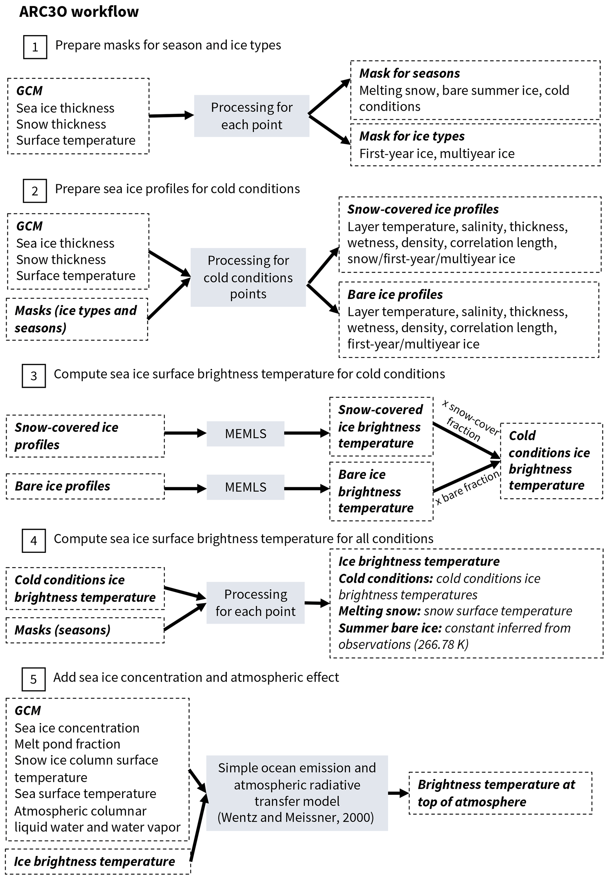
As a consequence, ARC3O is based on two parts. In the first part, an emission model computes the sea ice surface brightness temperature (see Sect. 3.1). In the second part, an atmospheric radiative transfer model combines the sea ice surface emission with ocean emission and atmospheric emission, reflection, and transmission (see Sect. 3.2). The workflow of ARC3O follows five steps (see Fig. 1), which we explain below.
3.1 The contribution of the sea ice surface to the brightness temperature
The brightness temperature TBice emitted at an ocean surface completely covered by sea ice at 6.9 GHz vertical polarization, is primarily driven by the vertical distribution of the brine volume fraction inside the ice, which principally depends on the temperature and salinity profile (see Burgard et al., 2020, for more details). However, MPI-ESM does not provide temperature and salinity profiles. To circumvent this lack of information, we follow the suggestion of Burgard et al. (2020) to build a simple model for these sea ice properties, based on the boundary conditions given by the GCM.
3.1.1 Identifying different periods and ice types
Burgard et al. (2020) showed that the simulation of sea ice surface brightness temperatures relies on different assumptions, depending on the conditions of the ice. A sea ice year can be divided into three periods: cold conditions, melting snow, and bare ice near 0 ∘C. Additionally, sea ice brightness temperatures depend on the ice type, for example, first-year or multiyear ice.
We therefore flag the different type of periods and different ice types based on the sea ice properties given by the MPI-ESM output (step 1 in Fig. 1). Grid cells containing melting snow are flagged as “melting snow periods”; grid cells containing bare ice in July, August, and September are flagged as “bare ice near 0 ∘C”; and the remaining grid cells are flagged as “cold conditions”. To flag the different grid cells as “first-year ice”, “multiyear ice”, and “open water only”, we consider the ice thickness evolution. If the ice thickness is zero, the ice type is set to open water only; if the ice thickness is larger than zero, but there has been at least one open-water-only time step in the year preceding the time step evaluated, the ice type is set to first-year ice. If neither of these apply, the ice type is set to multiyear ice. This is a simplification, assuming that there is no ice drift and that the ice present at one point in time and space will be the same (but older) ice later in time.
3.1.2 Cold conditions
In periods of cold conditions, Burgard et al. (2020) showed that the sea ice surface brightness temperature can be simulated using an emission model by assuming a linear vertical temperature profile and a function of depth for the salinity. They also showed that the uncertainty range does not vary substantially if the profiles are interpolated to 5, 7, or 10 layers. In this study, we choose to use 10 layers. We construct profiles (step 2 in Fig. 1), divided into 11 layers, namely 10 layers of ice and 1 layer of snow. The ice layers are equidistant, based on the ice thickness given by MPI-ESM, and the snow layer thickness is equal to the snow thickness given by MPI-ESM.
We construct temperature profiles based on the ice surface temperature given by MPI-ESM, which represents the temperature at the top of the snow and ice column. For each grid cell, we construct two sets of profiles. One set of profiles interprets the surface temperature as the snow surface temperature. This profile is a combination of two linear profiles, one in the snow, defined by the snow thermal conductivity, and one in the ice, defined by the ice thermal conductivity, based on the temperature Tice,surf at the interface between ice and snow inferred as follows:
with ks the thermal conductivity of snow (=0.31 W Km−1), ki the thermal conductivity of ice (=2.17 W Km−1), hs the snow thickness, hi the ice thickness, Tsnow,surf the temperature at the surface of the snow, and Tbottom the temperature at the bottom of the ice, set to −1.8 ∘C.
The other set of profiles interprets the surface temperature as the ice surface temperature and is a linear profile between surface and bottom temperature. The ice bottom temperature is taken as constant at −1.8 ∘C in both cases.
The salinity profile S is computed as a function of depth z, as formulated by Griewank and Notz (2015), based on the results of 1D simulations with the complex thermodynamic sea ice model SAMSIM and their comparison to observations. S is defined as follows for first-year ice:
with a=1.0964, , and c=4.41272, and as follows for multiyear ice:
with a=0.17083, b=0.92762, and c=0.024516.
We set the snow salinity to zero. Note, however, that the validity of this assumption is slightly uncertain as the lowest layer of the snow can be saline, especially above first-year ice (Barber et al., 1998; Shokr and Sinha, 2015; Nandan et al., 2017), enabling the presence of brine at the base of the snow.
The vertical profile of the ice density ρi is computed based on the vertical temperature T and salinity S profiles, with the following formula applied to each ice layer (Notz, 2005):
where Φb is the brine volume fraction:
Sb is the brine salinity:
ρw is the density of brine with the chemical composition of seawater at 0 ∘C (Eq. 3.8 in Notz, 2005):
and ρ0 is the density of pure ice (Pounder, 1965):
The density of the snow layer is set to 300 kg m−3, as in MPI-ESM (Giorgetta et al., 2013).
The vertical profile of the correlation length, a measure for the scatterer size (snow particles, brine inclusions, air bubbles), depends on the ice type. If the ice layer is in the upper 20 cm of first-year ice, the correlation length is set to 0.35 mm. If the ice layer is located below the upper 20 cm, the correlation length is set to 0.25 mm (Tonboe, 2010). For multiyear ice, the correlation length is set to 1.5 mm for all ice layers (Burgard et al., 2020). The correlation length of the snow layer is set to 0.15 mm (Tonboe, 2010).
The sea ice surface brightness temperature is simulated based on the temperature, salinity, density, thickness, and correlation length profiles described above. A slightly modified version of the Microwave Emission Model for Layered Snowpacks (MEMLS, Wiesmann and Mätzler, 1999) extended for sea ice (Tonboe et al., 2006) is used for the brightness temperature simulation. It relates the snow and ice properties to emission, absorption, and scattering of the microwave radiation in each layer. Hence, MEMLS simulates the path of the radiation through the ice and snow from bottom to top, resulting in a brightness temperature emitted at the surface.
MPI-ESM provides a snow cover fraction, which means that the ice is not always fully covered by snow. To account for the effect of both snow-covered ice and bare ice on the radiation, we simulate two sea ice surface brightness temperatures for each grid cell. One set of brightness temperatures is simulated using the temperature profiles computed through snow and ice, where the surface temperature given by MPI-ESM is interpreted as the snow surface temperature. The other set is simulated using linear temperature profiles computed through ice only, assuming that there is no snow cover on the ice and the surface temperature given by MPI-ESM is interpreted as the ice surface temperature (step 3 in Fig. 1). These surface brightness temperatures are then combined, weighted by the snow cover fraction given by MPI-ESM, resulting in one mean sea ice surface brightness temperature.
3.1.3 Melting snow
In spring, temperatures increase across the Arctic Ocean, leading to the melting of the snow covering the sea ice. Wet snow strongly affects the emitted microwave radiation. This effect mainly depends on the water content and on the density of the snow (Chang and Gloersen, 1975; Ulaby et al., 1986; Shokr and Sinha, 2015). However, these snow properties are not resolved in MPI-ESM. We therefore cannot use MEMLS to simulate the brightness temperature of the ice and snow column in this case. Instead, we use the following definition of the brightness temperature:
where ϵeff is the emissivity of the emitting part of the ice and snow column, i.e., the layers influencing the resulting radiation emitted at the surface, and Teff is the integrated temperature over this same emitting part (Hallikainen and Winebrenner, 1992; Tonboe, 2010; Shokr and Sinha, 2015). At 6.9 GHz, the emitting part of wet snow is a thin subsurface layer and the emissivity is close to 1 (Hallikainen et al., 1986; Lee et al., 2018). Following Eq. (9), we therefore assume that the brightness temperature of ice covered by melting snow is equal to the snow surface temperature.
3.1.4 Summer bare ice near 0 ∘C
In summer, after the snow has fully melted away, the salinity profile inside the ice cannot necessarily be represented by a simple function of depth. As the subsurface ice can be assumed to be isothermal close to 0 ∘C during summer, the brine volume fraction in the subsurface layer, i.e., in the upper few centimeters of the ice, increases and melt ponds form. Above a subsurface brine volume fraction of 0.2, the brightness temperature is proportional to the subsurface brine volume fraction (Burgard et al., 2020). The subsurface brine volume fractions above 0.2 can be interpreted as a measure for the melt pond fraction as they mean that the surface is very wet. For these warm conditions, the physical properties of the ice which is not covered by melt ponds are similar over the whole Arctic Ocean. Burgard et al. (2020) therefore suggest a very simple approach: use a constant brightness temperature for the ice surface fraction, i.e., the ice fraction not covered by melt ponds.
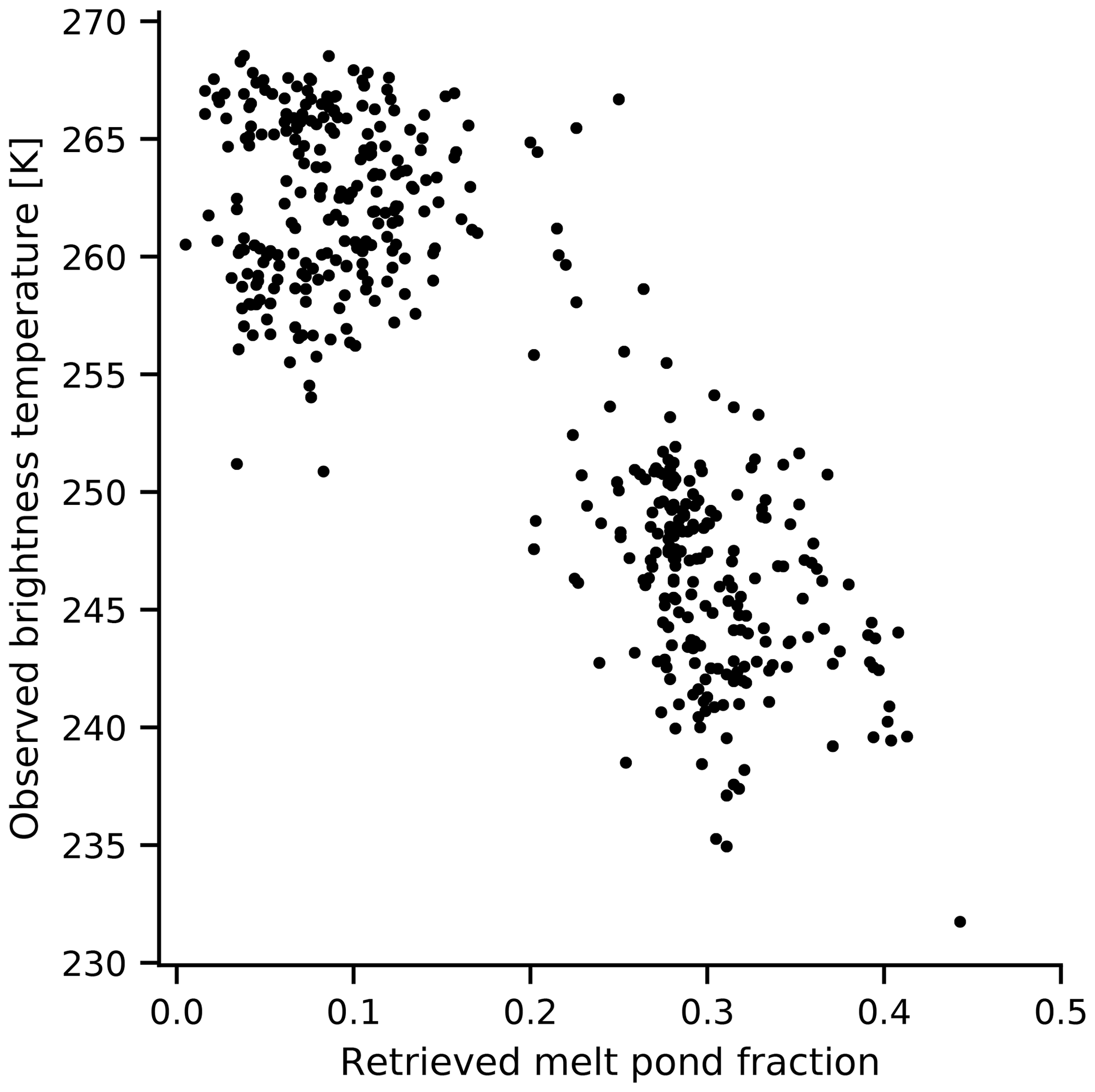
Figure 2Brightness temperatures measured by AMSR2 against the melt pond fraction product by Istomina et al. (2015b) for different points represented in the Round Robin Data Package from May to mid-August 2011.
To find a surface brightness temperature representing the sea ice surface in summer, we use the observational dataset Round Robin Data Package (RRDP, Pedersen et al., 2018) developed as part of the European Space Agency (ESA) sea ice Climate Change Initiative (SICCI). These data cover the period from May to mid-August 2011. The RRDP contains amongst others microwave brightness temperatures between 6 and 89 GHz measured by the Advanced Microwave Scanning Radiometer 2 (AMSR2) collocated with the melt pond fraction product by Istomina et al. (2015b) over areas estimated to be close to 100 % sea ice concentration. Using the combination of the melt pond fraction and the brightness temperatures measured from space, we can infer the summer brightness temperature of melt-pond-free sea ice (Fig. 2). Burgard et al. (2020) showed that, above a brine volume fraction of 0.2 in the upper few centimeters of ice, the brightness temperature is proportional to this subsurface brine volume fraction. We assume that melt ponds have the same effect as high subsurface brine volume fractions. Below 0.2, the effect of the ice on the brightness temperature is stronger than the effect of melt ponds. Therefore, to infer an ice brightness temperature for non-ponded ice, we take the mean brightness temperature of ice covered by 20 % or less melt pond. This method results in a summer ice brightness temperature of 262.29±3.56 K at the top of the atmosphere. After applying an atmospheric correction (see Sect. 3.2), the resulting summer ice brightness temperature at the surface is 266.78 K.
3.2 The contribution of ocean and atmosphere to the brightness temperature
As the Arctic Ocean is not covered 100 % by sea ice, the brightness temperature measured at the top of the atmosphere is also influenced by the relative fraction and properties of open-water surfaces and properties of the atmosphere. To take into account these oceanic and atmospheric contributions, we use a geophysical model developed by Wentz and Meissner (2000) (step 5 in Fig. 1).
In this geophysical model, the total brightness temperature of an Arctic Ocean grid cell is computed as a combination of the upwelling surface emission by ocean, sea ice, and melt ponds; the upwelling atmospheric emission; the atmospheric transmittance; the atmospheric emission reflected by the different types of surface; and the reflected background radiation from space. The ocean surface brightness temperature is computed as a function of surface temperature, surface salinity, and wind speed. The melt pond brightness temperature is computed similarly to the ocean brightness temperature but by setting salinity and wind speed to zero. Finally, as the atmosphere is mostly transparent to radiation in the low microwave range, the radiative transfer through the atmosphere is computed based only on the columnar water vapor and columnar cloud liquid water.
The sea ice surface brightness temperature used as input for this geophysical model is set for each grid cell depending on the three periods presented above (step 4 in Fig. 1). The sea ice surface brightness temperature is computed by MEMLS (see Sect. 3.1.2) in cold conditions and approximated with the snow surface temperature in conditions of melting snow (see Sect. 3.1.3). In summer, however, our method was based on brightness temperatures as measured by satellites from space and therefore resulted in a sea ice brightness temperature for the top of the atmosphere. To obtain a sea ice brightness temperature at the surface that can be used as input for the combination of ocean and sea ice surface brightness temperature for summer conditions, we need to apply an atmospheric correction.
To infer a mean atmospheric correction, we apply the geophysical model to regions covered 99 % or more by sea ice in MPI-ESM output presented in Sect. 4.2, setting all melt pond fractions to zero. This way, we have no influence from open-water surfaces, be it ocean or melt ponds, on the resulting brightness temperature. We set the ice surface brightness temperature used as input for the geophysical model to a random constant. We then subtract this constant ice surface brightness temperature from the top-of-the-atmosphere brightness temperature simulated by the geophysical model based on atmospheric properties given by the climate model output. This gives us a mean atmospheric effect of 4.49 K. We add this to the brightness temperature of 262.29 K inferred in Sect. 3.1.4, resulting in a constant brightness temperature of 266.78 K as a constant brightness temperature representing the radiation emitted at the summer bare ice surface. This is the bare ice summer surface brightness temperature that can be used for combination with open-water (ocean and melt ponds) brightness temperature in the geophysical model in step 5 of Fig. 1.
The approach we use to construct ARC3O was proposed by Burgard et al. (2020), based on an idealized one-dimensional setup that did not involve actual observations. In the following, we evaluate our simulated Arctic Ocean brightness temperatures against brightness temperatures measured by satellites.
We do so by comparing brightness temperatures simulated by ARC3O based on MPI-ESM output from assimilation experiments, i.e., experiments where the model is regularly nudged towards observations. Hence, we expect the simulated climate system to be close to reality and the simulated brightness temperature to be close to the observed brightness temperature.
However, the observations used in the data assimilation are reanalysis data for the atmosphere and ocean and retrieved sea ice concentration products for the sea ice. They are therefore not direct observations but already processed products prone to differences to reality. Additionally, in the assimilation process, MPI-ESM is nudged towards observations, but some characteristic features inherent to the mean model state might remain. This is the case when the mean model state and the assimilated state are so incompatible that the model will rapidly drift back towards the mean model state. The uncertainty of the measured brightness temperature itself is around 1 K (NASDA, 2003) and thus neglected here. Hence, differences between observed and simulated brightness temperature can arise from three sources: (1) the difference between real and retrieved climate state due to the difference between retrieval algorithms or reanalysis and the real climate state, (2) the difference between the assimilated climate state and the retrieved or reanalysis product, and (3) biases in ARC3O (Fig. 3). In the following, we try to quantify how the first two uncertainty sources contribute to differences between the simulated and observed brightness temperatures. Any remaining biases can then be attributed to biases of ARC3O itself.

Figure 3Uncertainty sources possibly introducing differences between simulated and observed brightness temperature.
4.1 Observation data
As observed brightness temperatures, we use Calibrated Passive Microwave Daily EASE-Grid 2.0 (CETB) brightness temperatures processed as part of the NASA Making Earth System Data Records for Use in Research Environments (MEaSUREs) program (Brodzik et al., 2016). They are an improved, enhanced-resolution, gridded passive microwave Earth System Data Record (ESDR) for monitoring cryospheric and hydrologic time series from the measurement devices Scanning Multi-channel Microwave Radiometer (SMMR), Special Sensor Microwave Imager/Sounder (SSM/I-SSMIS), and Advanced Microwave Scanning Radiometer – Earth Observing System (AMSR-E). These data cover the period between 1978 and 2017 and are provided on a 25 km×25 km grid. For the comparison with MPI-ESM data, we focus on the period from 2002 to 2008 and interpolate the observations bilinearly to the model grid (). Again, we concentrate on the frequency of 6.9 GHz vertical polarization. At this frequency and this time period, the observations stem from AMSR-E.
4.2 Model data
We use model data from assimilation runs, as they are nudged towards the observed climate state and are therefore expected to be a reasonable estimate of the real climate state in the model. Differences between simulated and observed brightness temperatures should therefore be small and can be attributed to the three uncertainty sources presented before (see Fig. 3). To examine the impact of the choice in sea ice retrieval product, we use three assimilation runs based on three different sea ice concentration products. The atmosphere and the ocean component are assimilated in the same way in all three cases.
The assimilation experiments cover the period from 2002 to 2008 and were conducted by Bunzel et al. (2016). The assimilation technique used was Newtonian relaxation, also called nudging. Atmospheric, oceanic, and sea ice properties were nudged into the model using full-field data assimilation in all atmospheric and oceanic levels. In the atmosphere, vorticity, divergence, temperature, and surface pressure were nudged into the model with a relaxation time of 1 d, while salinity and temperature in the ocean were nudged with a relaxation time of 10 d. For the assimilation of atmospheric quantities, the ERA-Interim dataset (Dee et al., 2011) was used, while the ocean was nudged toward Ocean Reanalysis System 4 data (Balmaseda et al., 2013).
For sea ice, only sea ice concentration was assimilated. The three different sea ice concentration products are the ESA SICCI Version 2 (SICCI2) dataset (Lavergne et al., 2019), as a 50 km gridded product, and the NASA Team dataset (Cavalieri et al., 1996) and the Bootstrap dataset (Comiso, 2000), both as 25 km gridded products. We choose these datasets because SICCI2 is a new algorithm combining several existing algorithms with the goal of improving the retrieved sea ice concentration product, Bootstrap sea ice concentrations are in the upper range of retrieved sea ice concentrations, and NASA Team sea ice concentrations are in the lower range (Ivanova et al., 2014; Kern et al., 2019). The data were interpolated bilinearly to the model grid before assimilation. In grid boxes containing missing values, e.g., the polar observation hole (northward of 87.2∘ N), no assimilation was applied. The sea ice was then exclusively calculated by the model. To avoid brightness temperature uncertainties due to this free simulation region, we mask out the region northward of 86.72∘ N, the highest latitude on our grid below the observational hole. The relaxation time was 20 d. Relaxation times differ among the model components to account for the different response times of the components. In order to allow for a realistic relation between ice concentration SIC and thickness h, sea ice thickness was updated in the model proportionally to ice concentration nudging (Tietsche et al., 2013). The assimilation changes the thickness h in the given grid cell by Δhassim, which is proportional to ΔSICassim, with a proportionality factor h* of 2 m, as follows:
4.3 Cold seasons (JFM, AMJ, OND)
4.3.1 Comparison between simulated and observed brightness temperatures
The first comparison between simulated and observed brightness temperatures clearly showed a positive bias over the whole Arctic Ocean in the simulated brightness temperatures (Fig. A1a). The brightness temperature is defined as the product of the emissivity and the physical temperature of the emitting part of the ice (Ulaby et al., 1986). A comparison of the simulated emissivities with emissivities derived from observational data from the RRDP showed that ARC3O systematically overestimates the emissivity. It is, however, not straightforward to find where the bias is produced in the emission model. We therefore chose to correct the bias by multiplying the inherent sea ice emissivity by a tuning coefficient at the end of step 3 of the ARC3O workflow (see Fig. 1). The coefficient that yields the best agreement with observations is 0.968 (Fig. A1b). More information about the tuning process is found in Appendix A. In the following, we discuss brightness temperatures simulated with this tuning procedure.
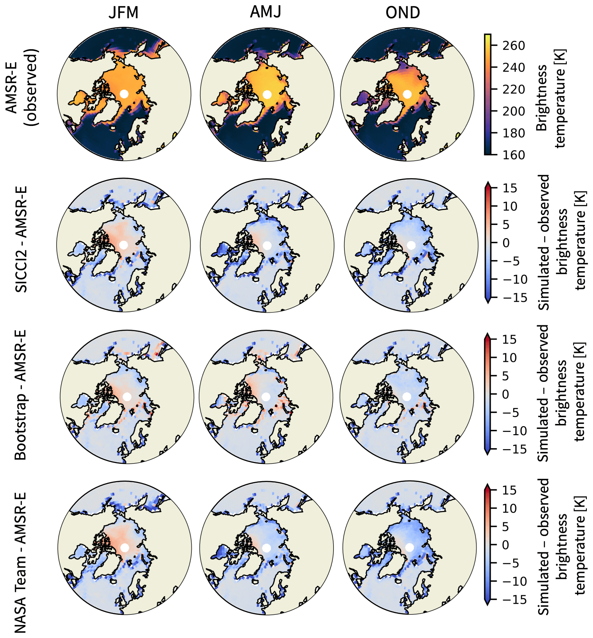
Figure 4Observed brightness temperatures by AMSR-E (top row). Differences between brightness temperatures simulated with ARC3O from MPI-ESM output assimilated with SICCI2 (second row), Bootstrap (third row), and NASA Team (bottom row) sea ice concentration and observed brightness temperatures. The columns stand for the three cold seasons: JFM, AMJ, and OND. Summer (JAS) is discussed in Sect. 4.4.
The three different sets of simulated brightness temperatures show largely similar behaviors in the cold seasons, i.e., winter (January, February, March, JFM), spring (April, May, June, AMJ), and autumn (October, November, December, OND) (Fig. 4). Overall, differences between simulated and observed brightness temperatures are very small and are generally lower than 10 K. The pattern of differences appears to be similar across seasons. The simulated brightness temperatures are slightly higher than the observed ones in regions of high sea ice concentration and thickness, e.g., north of the Canadian Archipelago and the central Arctic in winter. In contrast, they are lower than the observed ones in regions of low sea ice concentration and thickness, e.g., in the marginal zones such as the Barents Sea, the Pacific sector, and Hudson Bay, in the brightness temperature simulations based on the SICCI2 and NASA Team assimilation runs and higher in the brightness temperature simulation based on the Bootstrap assimilation run.
The overestimation on the order of 2 to 4 K in the central Arctic in winter has a similar pattern in all three sets of simulated brightness temperatures. Otherwise, brightness temperatures simulated based on the Bootstrap assimilation run are very close to the observed ones, with differences to the observations of usually less than 3 K. Only a few individual points in the Atlantic sector show larger biases. Brightness temperatures simulated based on the NASA Team and SICCI2 assimilation run show stronger differences to observations. The simulated brightness temperatures are up to 10 K lower than the observations in the North Pacific in winter and up to 15 K lower than the observations in Hudson Bay in spring. In the central Arctic and the Atlantic sector, the brightness temperatures simulated based on the NASA Team assimilation run are 2 to 5 K lower than observations in spring and 5 to 10 K lower than observations in autumn. The pattern of differences between brightness temperatures simulated based on SICCI2 assimilation run and observations is similar to the pattern of differences between brightness temperatures simulated based on the NASA Team assimilation run and observations, but the brightness temperatures simulated based on the SICCI2 assimilation run are about 2 K higher than the brightness temperatures simulated based on the NASA Team assimilation run.
4.3.2 Investigating uncertainty sources
The total difference Δtot between simulated and observed brightness temperatures is a consequence of the difference between real and retrieved climate state Δretriev, of the difference between retrieved and simulated climate state Δassim, and of biases in the brightness temperature simulation by ARC3O ΔARC3O (Fig. 3):
We set out to investigate Δassim and Δretriev to gain an estimate of ΔARC3O.
In a first step, we investigate which drivers the brightness temperature is particularly sensitive to. We concentrate on the variables provided by MPI-ESM, as these are the ones we can quantify in our setup. In the cold seasons, the most important drivers for the simulation of a brightness temperature for a surface covered by varying fractions of sea ice and open water are the sea ice concentration, sea ice thickness, snow thickness, and surface temperature.
We examine the sensitivity for the month of October, representing the beginning of the freezing period, and for the month of March, representing the end of the freezing period. We do so for the SICCI2, the Bootstrap, and the NASA Team assimilation runs. As the results of the analysis are similar for all three assimilation runs unless otherwise mentioned, we only show the results for the SICCI2 assimilation run in the following.
We start by estimating the internal variability for each variable at a given date and at a given grid cell. For each date in October and March, we compute the standard deviation over a sample of 5 years (2003 to 2008) for each variable and each grid cell. As an overview, the range and the time mean of the resulting variabilities are shown in Table 1 (first column) and in Fig. B1, respectively.
Table 1 Sensitivity of the simulated brightness temperature to different input variables of the simulation. We show the spatial 5th and 95th percentile of the time mean of the estimated variability for the variables of interest (also see Fig. B1) in the first column. We show the spatial 5th and 95th percentile of the time mean difference between modulated and reference brightness temperature when the variability field is added to (second column) and subtracted from (third column) the reference field. These values are inferred from the SICCI2 assimilation run.
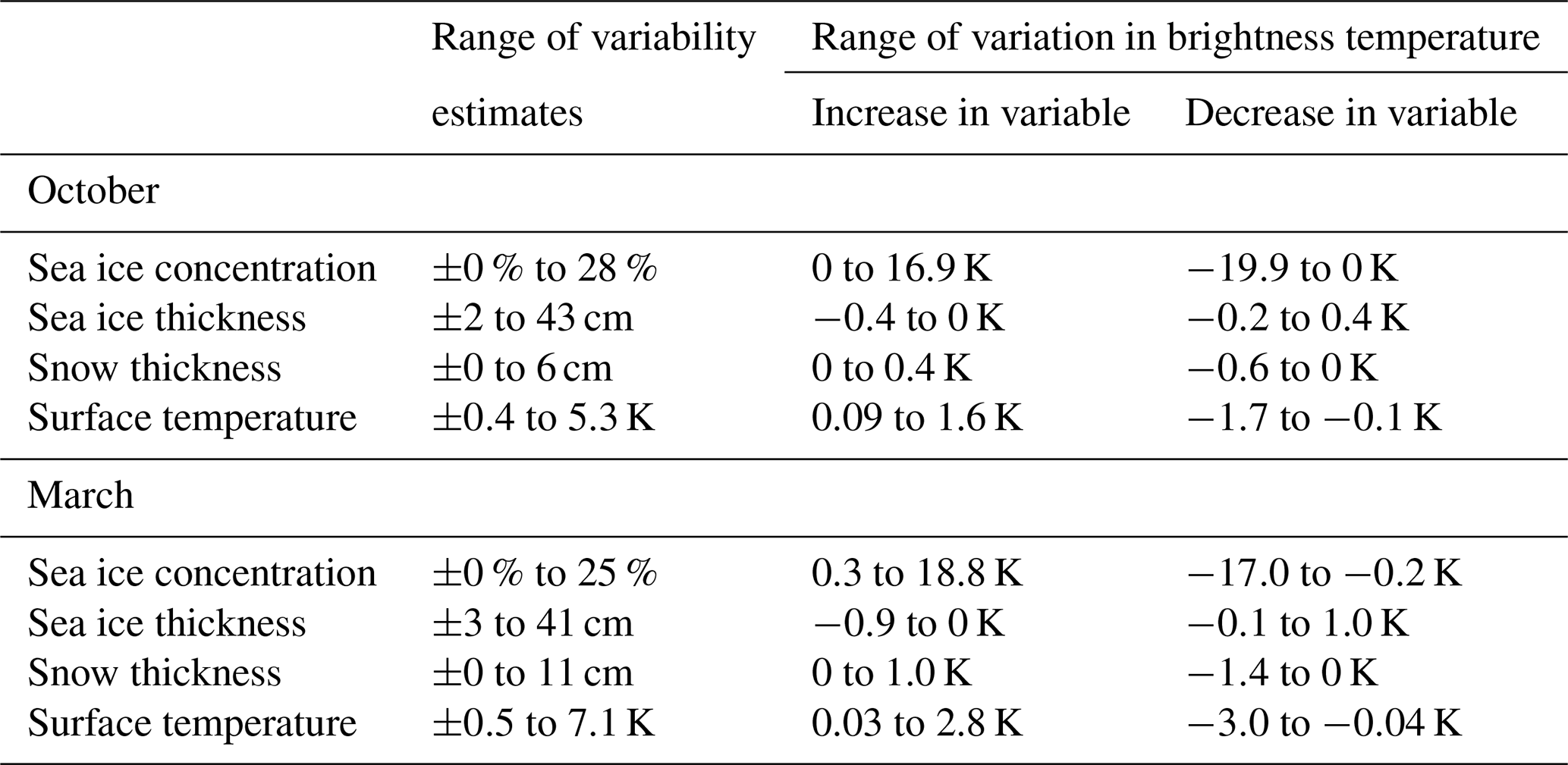

Figure 5The variables that have the highest absolute mean effect on the brightness temperature in October (a) and March (b) when their variability field (see Table 1 and Fig. B1) is added to (first and third columns) and subtracted from (second and fourth columns) the input variable. These results are inferred from the SICCI2 assimilation run. Inspired by Fig. 5 in Richter et al. (2018).
With these variability fields, we conduct sensitivity studies for each variable of interest. For both October and March, we conduct two sets of experiments per variable of interest, one in which we add the variability field to the variable of the reference assimilation run and one in which we subtract the variability field. Ranges of the difference between the resulting brightness temperatures and the brightness temperatures simulated based on the reference assimilation run are shown in Table 1 (second and third columns). The main message emerging from the results is that the sea ice concentration variability is the driver for the largest variations in the brightness temperature, changing it by up to nearly 20 K, while the variability in other variables affects the brightness temperature only up to 3 K. Spatially, the sea ice concentration is the main driver for variability in regions not completely covered by ice (Fig. 5). In regions covered nearly 100 % by ice, the surface temperature has the highest effect on the brightness temperature. Although they both have an indirect influence on the ice surface temperature as well, sea ice thickness and snow thickness do not play, except very locally, an important role for uncertainties in the total brightness temperature of a grid cell in the simulated variability range, as their mean absolute contribution to the brightness temperature variability is on the order of 1 K.
In the sensitivity study using the NASA Team assimilation run, the variability ranges of sea ice thickness and surface temperature are comparable to the other runs (not shown). However, the sea ice thickness is the main driver of variability for a large region in the central Arctic north of Alaska in March (not shown). Further investigation into these differences in the main driver for the brightness temperature could lead to a better understanding of the differences in the simulated climate of these three assimilation runs. However, this is beyond the scope of our study and is a subject for future work.
In summary, this sensitivity study shows that sea ice concentration and surface temperature are the dominant drivers of variability in the simulated brightness temperature. To understand the total uncertainty Δtot, we therefore need to focus on these two variables.
In a next step, we investigate the influence of Δassim on Δtot. The goal of a data assimilation is to reach a simulated climate state close to reality. During the data assimilation process, the model is nudged towards three distinct observational datasets: an ocean reanalysis, an atmosphere reanalysis, and a sea ice concentration product, which are not necessarily consistent with each other. Hence, discrepancies can arise between the variables before and after the assimilation. This is the case, for example, when a nonzero sea ice concentration is assimilated at one point but the ocean temperature is too warm to sustain the ice at that point and thus the ice directly melts away.
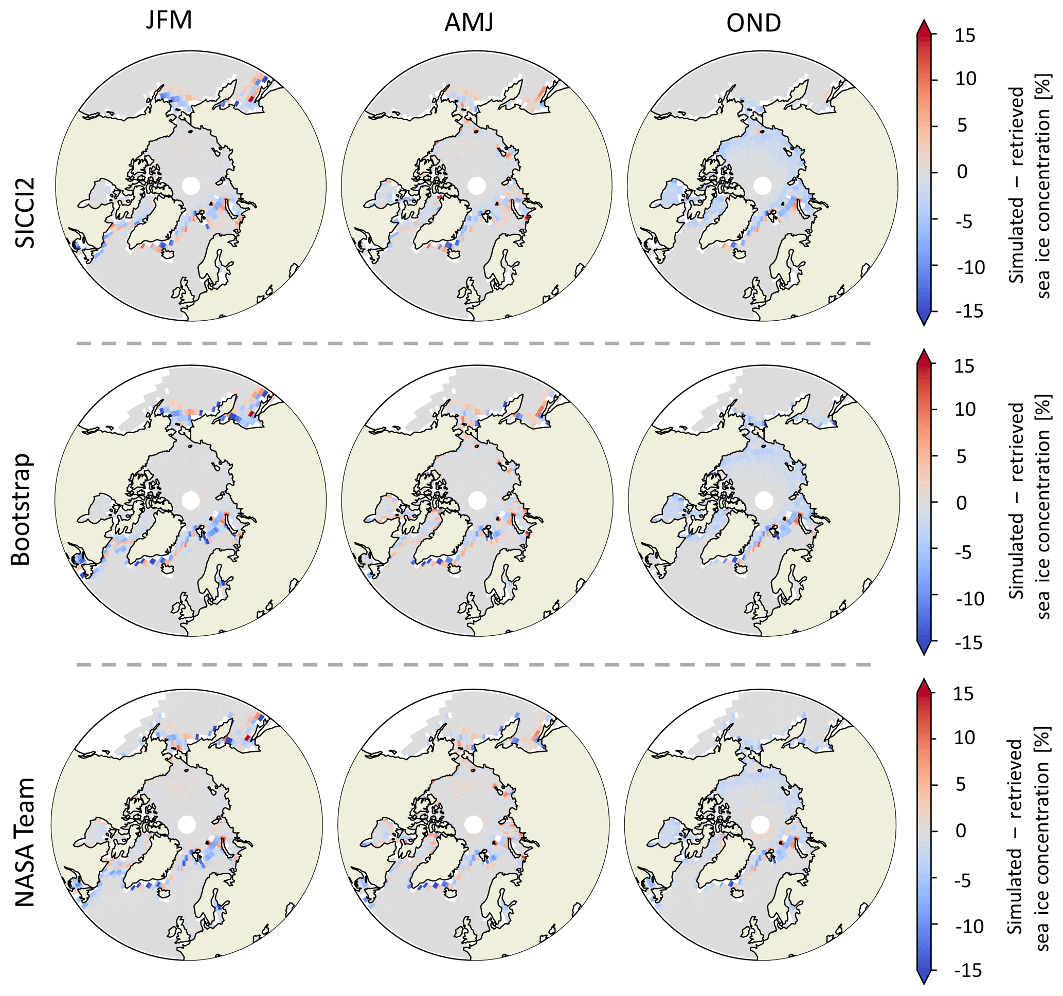
Figure 6Difference between retrieved (before data assimilation) and simulated (after data assimilation) sea ice concentration for the three assimilation runs.
As the sea ice concentration is the main driver for uncertainties in the brightness temperature simulation, we focus here on the effect of the data assimilation procedure on the sea ice concentration in the three different assimilation runs. This effect is mostly visible in the marginal regions (Fig. 6) and is of similar magnitude for all three assimilation runs. At the ice edge, the differences between the original sea ice concentration observational product and the sea ice concentration assimilated in the simulation are highest, on the order of 5 %. As a rule of thumb, differences of 1 % in sea ice concentration are equivalent to differences of 1 K in brightness temperatures (see Burgard et al., 2020), so the differences in sea ice concentration are roughly equivalent to resulting differences in brightness temperature of around 5 K. Δassim can therefore account for a large part of the total difference between simulated and observed brightness temperature Δtot in the ice edge region (see Fig. 4).
Unfortunately, the difference between real and retrieved sea ice concentration Δretriev cannot be as robustly quantified as Δassim. In situ observations for a robust evaluation of the retrieved sea ice concentration products are largely lacking. Although there have been local evaluation approaches, based on regions known to be 100 % covered by sea ice (e.g., Ivanova et al., 2015; Tonboe et al., 2016; Lavergne et al., 2019), this lack of in situ observations inhibits the evaluation of the products on larger scales against reality. The effect of Δretriev and ΔARC3O can therefore not clearly be disentangled.
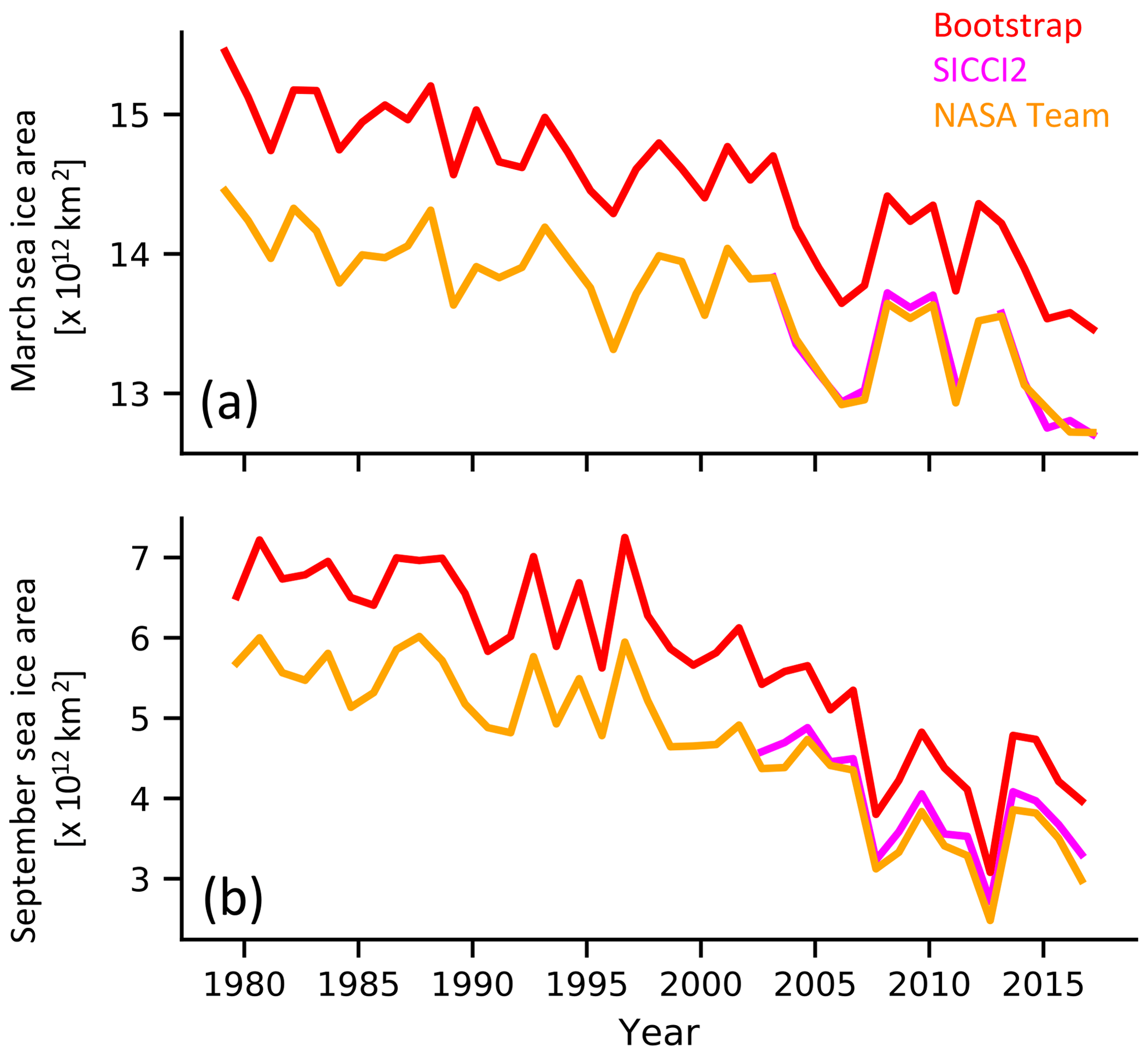
Figure 7March (a) and September (b) sea ice area for the three observational datasets assimilated in the three assimilation runs used.
Still, we can give an estimated range for ΔARC3O. To do so, we use the spread between the SICCI2, Bootstrap, and NASA Team sea ice concentrations as an estimate of the uncertainty range around the real sea ice concentration (Fig. 7 and Ivanova et al., 2014; Kern et al., 2019). First, we subtract Δassim from the simulated brightness temperature. Δtot is now only a sum of Δretriev and ΔARC3O. Second, for each grid cell and each time step, we evaluate if the observed brightness temperature is located within the range of the brightness temperatures simulated based on the three different sea ice concentration products. If yes, differences are not necessarily a bias induced by ARC3O. If not, it is likely that ARC3O induces a bias. In this case, the simulated brightness temperature with the lowest absolute distance from the observed brightness temperature represents the smallest plausible estimate of ΔARC3O (Fig. 8, second row). The largest absolute difference between simulated and observed brightness temperatures in contrast gives an estimate of the largest plausible value of ΔARC3O (Fig. 8, third row). If the observed brightness temperature is within the range obtained for the different retrieved sea ice concentration estimates, the estimate of ΔARC3O is set to zero.
The resulting mean estimates of ΔARC3O are both very small, as the minimal estimates are well below 5 K and the maximal estimates are 5 K or below, except in Hudson Bay. Additionally, the comparison of the ΔARC3O estimates to the spread in sea ice concentration between Bootstrap and NASA Team (Fig. 8, fourth row) shows that biases in ARC3O, i.e., ΔARC3O, are small compared to the uncertainty in retrievals, i.e., Δretriev, except in the central Arctic on the Canadian side.
The overestimation on the Canadian side of the central Arctic is likely due to a MPI-ESM bias in the sea ice thickness. The sea ice thickness in our assimilation runs is on the order of 2 m at its thickest north of the Canadian Archipelago (not shown). Observational estimates tend to instead show thicknesses of 3 to 4 m in this region (Ricker et al., 2017). This is much more than the thickness variability used in our sensitivity study and points to a possible stronger influence of sea ice thickness on the difference between simulated and observed brightness temperature than was estimated from the sensitivity study in this case.
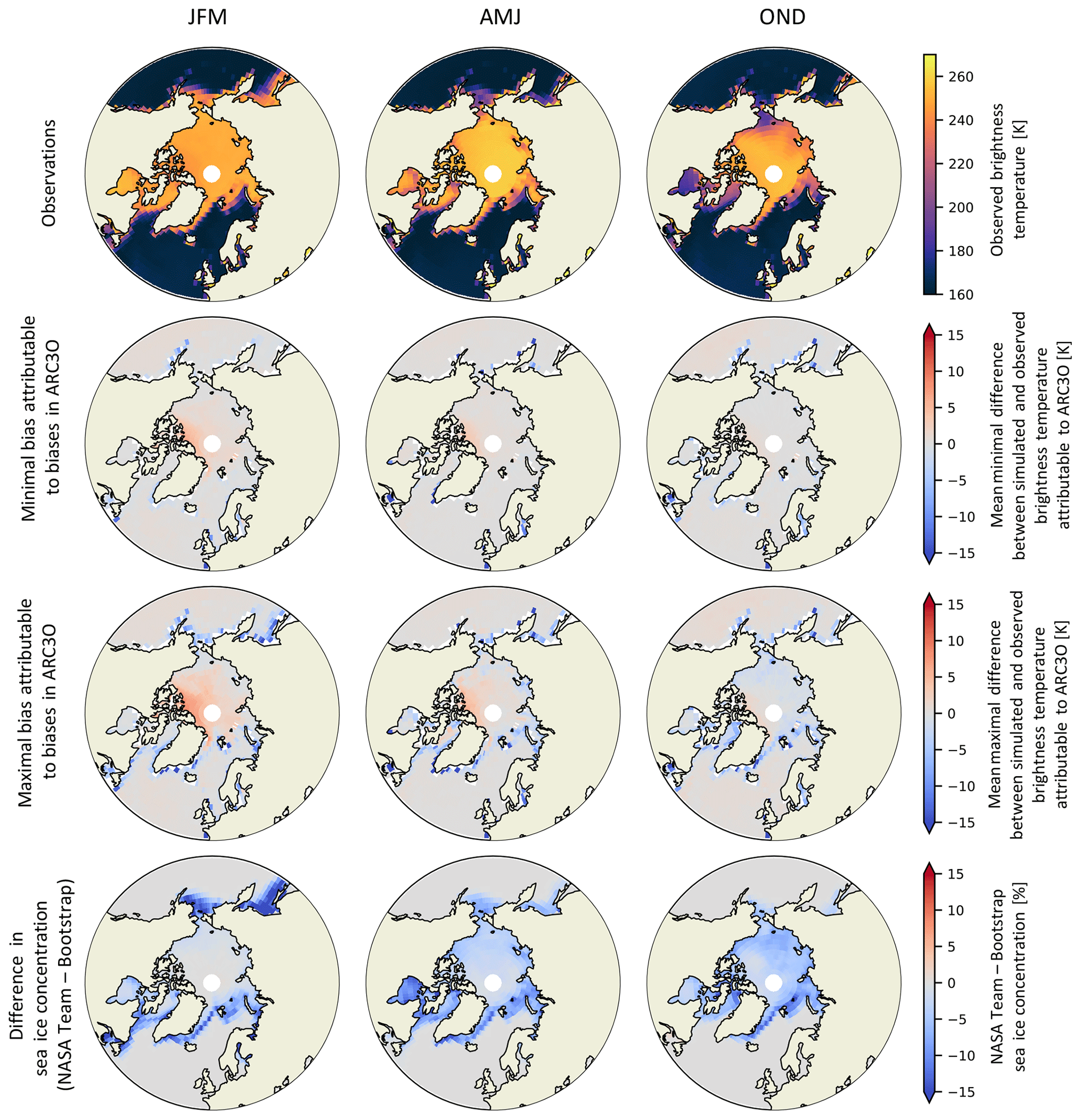
Figure 8Observed brightness temperatures (first row), mean minimal (second row) and mean maximal (third row) estimates of ΔARC3O, and differences in sea ice concentration (fourth row) between the NASA Team and Bootstrap assimilation runs, i.e., maximal estimates of Δretriev.
The remaining uncertainty contained in ΔARC3O can have several sources: ARC3O itself, further biases in the simulated climate state, or incorrect assumptions in our approach. Biases in ARC3O itself can arise from wrong assumptions in the sea ice emission model MEMLS or in the ocean emission and atmospheric transfer model by Wentz and Meissner (2000). For example, the brightness temperatures simulated over open ocean by ARC3O tend to be around 3 K too low. More investigation and fine-tuning above the open ocean might therefore slightly lower the uncertainty introduced by ARC3O. Another example is the approach to define first-year and multiyear ice in the ARC3O framework. The definition we use does not take into account the dynamics of the ice. As a consequence, if a grid cell is located in a region where sea ice circulates horizontally and therefore contains ice for more than a year, the ice in this grid cell will be defined as multiyear ice. This is the case even if the ice transported through the grid cell is not the same physical ice floe throughout this time period but a different first-year ice floe every day, for example. Rethinking this definition, e.g., by finding a way to follow the movement of the ice in the climate model, might therefore also reduce the uncertainty.
Concerning the simulated climate state, we expect small biases for the simulated surface temperature because the ERA-Interim reanalysis compares well to the few available in situ observations (Lindsay et al., 2014) and satellite-retrieved temperature measurements could be used if further evaluation was needed. We currently cannot explore the additional impact of model biases in sea ice thickness and snow thickness, as in situ observations are rare and satellite retrievals of these variables are not necessarily robust yet. Observational estimates for sea ice and snow thickness are mainly based on retrieval algorithms, similar to sea ice concentration estimates. Possible biases may therefore remain in these variables compared to reality.
Finally, we treat the spread between the SICCI2, Bootstrap, and NASA Team sea ice concentrations as an estimate of the uncertainty range around the real sea ice concentration. Hence, we implicitly assumed that the real sea ice concentration lies in the range between the SICCI2, the Bootstrap, and the NASA Team estimates. As only limited evaluation against reality is possible, the real sea ice concentration could lie outside of this range, and the uncertainty between real and retrieved sea ice concentration might be different to what we assume here.
As a conclusion, we showed in the consistent model setup that the sea ice concentration is the main driver for large variations in the brightness temperature in regions that are not fully ice-covered. In regions where the sea ice concentration is very high and does not vary much, such as the central Arctic in winter, the surface temperature is the main driver of variations in the brightness temperature. Simulated and observed brightness temperatures are generally in good agreement. Most differences are likely driven by the uncertainty brought by the sea ice concentration products compared to reality. Remaining differences attributable to biases in ARC3O remain below 5 K.
The lack of evaluation possibilities for the observation operator is an indicator for how little is actually known about the real Arctic climate state and processes at work, in particular in regard to the real sea ice concentration and surface temperature. Extending this observation operator to lower and higher frequencies would be of advantage to fill this gap. Brightness temperatures at different frequencies and polarizations are sensitive to different particular parameters. The combination of different brightness temperatures could enable a comprehensive assessment of the Arctic Ocean surface and atmosphere, and a comprehensive evaluation of the individual observation operators. For example, using an observation operator applied to reanalysis data, Richter et al. (2018) simulated brightness temperatures at the frequency of 1.4 GHz. They found that sea ice concentration and surface temperature are the main drivers for variations in the brightness temperature in the central Arctic but that in regions of thin ice the ice thickness is the dominating driver at this frequency. Combining frequencies in this case would then enable a climate model evaluation encompassing different perspectives.
4.4 Melting season (JAS)
As in winter, the simulated summer brightness temperatures are primarily a function of sea ice concentration. Melt ponds are then the main challenge for sea ice retrieval algorithms, as their passive microwave signature is undistinguishable from open water. This leads to large uncertainties and potential underestimation of the sea ice concentration in summer (Cavalieri et al., 1990; Comiso and Kwok, 1996; Fetterer and Untersteiner, 1998; Meier and Notz, 2010; Rösel et al., 2012b; Kern et al., 2016). The difference between observed and simulated brightness temperature (Fig. 9, second row) and the differences between observational sea ice concentration products are therefore much larger in summer than in winter (Ivanova et al., 2015; Kern et al., 2016).
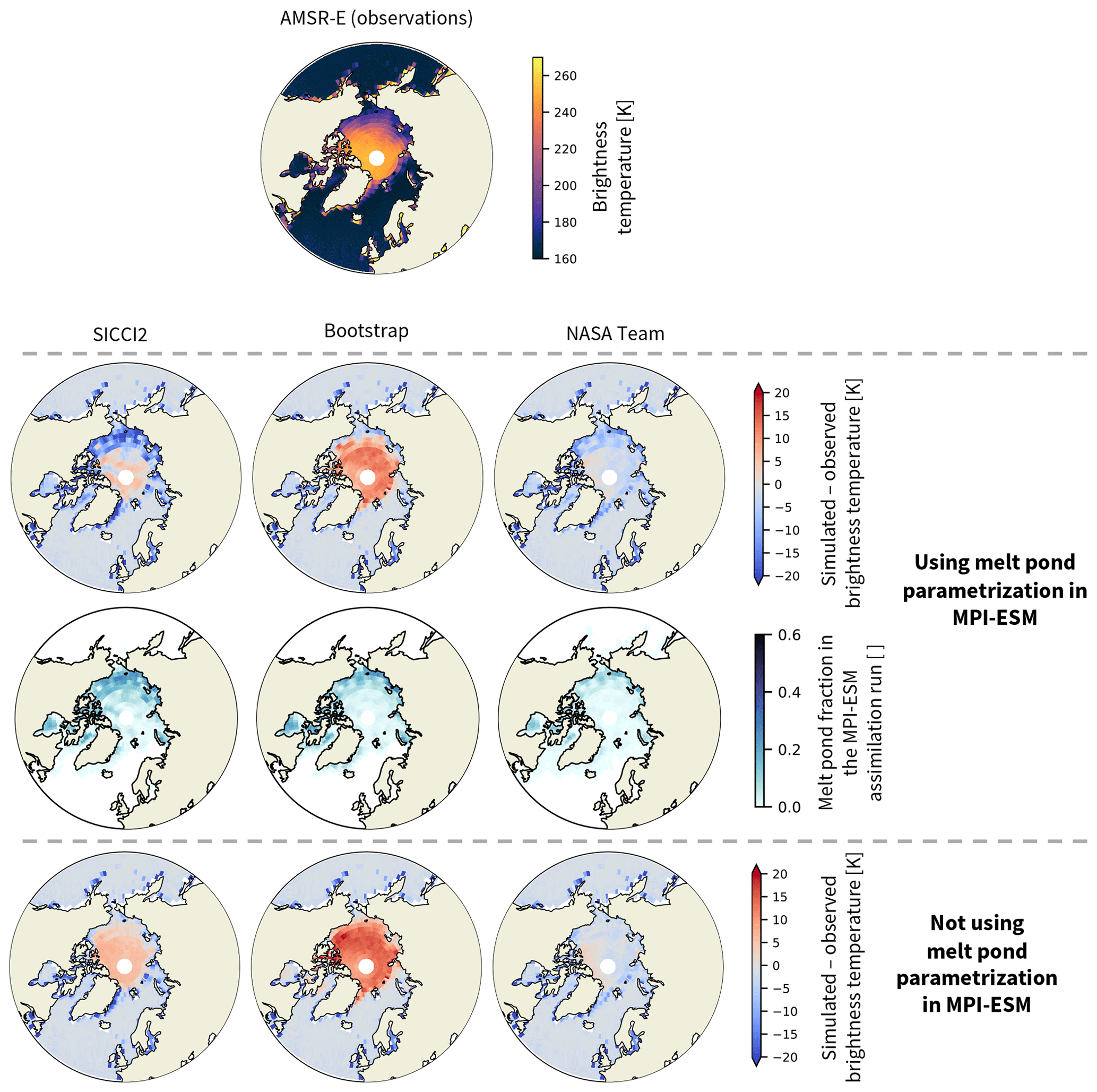
Figure 9Experiment to compare brightness temperatures in summer (July–August–September) simulated based on assimilation runs assimilated with different sea ice concentration products (SICCI2, Bootstrap, NASA Team) to brightness temperatures measured by AMSR-E. Observations by AMSR-E are shown in the first row. The difference between simulated and observed brightness temperatures if melt ponds are taken into account (second row) and if they are set to zero (fourth row) is shown. In the third row, the melt pond fraction simulated by MPI-ESM is shown.
In summer, the simulation of brightness temperatures in ARC3O is only based on the combination of a constant bare ice brightness temperature and melt pond brightness temperature, weighted by the melt pond fraction. The constant bare ice brightness temperature of 266.78 K is derived by using observed brightness temperatures and melt pond fractions, as explained in Sect. 3.1.4). Assumptions about the chosen constant ice surface brightness temperature can influence the analysis but we assume that the uncertainty between simulated and observed brightness temperatures in summer is mainly driven by two parameters: the difference between real and retrieved sea ice concentration and the difference between real and simulated melt pond fraction.
In the following, we can therefore evaluate the sea ice concentration products in summer and their relationship to the melt pond fraction. To do so, we distinguish between two types of sea ice concentration: the total sea ice concentration and the pond-free sea ice concentration. The pond-free sea ice concentration is the concentration of sea ice visible by the satellite, assuming that melt ponds are open water. In MPI-ESM, we know both the total sea ice concentration and the pond-free sea ice concentration, as melt ponds are represented through a melt pond parametrization, which is a function of the surface energy budget and water drainage to the ocean (Roeckner et al., 2012). In the SICCI2 algorithm, melt ponds are not explicitly accounted for, but the dynamic tie points are based on observed brightness temperatures in areas of high sea ice concentration, which are covered by melt ponds in summer. The retrieved sea ice concentration will therefore implicitly account for the melt ponds, potentially reducing the underestimation of the sea ice concentration (Kern et al., 2016; Lavergne et al., 2019). In the Bootstrap algorithm, a correction is applied to the sea ice concentration to account for the effect of melt ponds by synthetically increasing the retrieved sea ice concentration (Comiso and Kwok, 1996; Bunzel et al., 2016), while in the NASA Team algorithm, no correction is applied (Comiso et al., 1997; Bunzel et al., 2016). By switching the melt pond parametrization in MPI-ESM on and off, we can evaluate the ability of observational products to produce a reasonable pond-free and total sea ice concentration.
In this experiment, we run ARC3O on the three MPI-ESM assimilation runs, setting the melt pond fraction to zero everywhere. We then compare this set of simulated brightness temperatures to observed brightness temperatures (Fig. 9, fourth row) and to the set of brightness temperatures simulated taking into account the melt pond distribution simulated by MPI-ESM (Fig. 9, second row). The results give different insights depending on the sea ice concentration product used for the assimilation.
Using the SICCI2 assimilation run, the simulated brightness temperature of the pond-free sea ice is higher than the observed brightness temperature in the central Arctic. Melt ponds cover the whole ice-covered Arctic Ocean (Rösel et al., 2012a; Istomina et al., 2015a). Adding their effect in the brightness temperature simulation could therefore reduce the difference between simulated and observed brightness temperature. However, while the melt pond parametrization in MPI-ESM reduces the overall brightness temperature, the reduction is very heterogeneous, and thus the brightness temperature is now largely underestimated in the Pacific sector but still overestimated in most of the central Arctic. This means that the dynamic tie point approach of the SICCI2 algorithm seems to take into account the effect of melt ponds in a reasonable way, therefore yielding a pond-free sea ice concentration that is too high. The brightness temperatures simulated using the melt pond parametrization suggest that SICCI2 does not represent the total sea ice concentration well. However, the melt pond distribution in MPI-ESM seems to be too heterogeneous and therefore unrealistic in some regions, as most simulated melt ponds concentrate in the Pacific sector and not many can be found over the central Arctic (see Fig. 9, third row, and Roeckner et al., 2012). The latitudinal gradient is realistic, showing more melt ponds in lower latitudes, where the incoming solar radiation and air temperatures are higher, than in higher latitudes. However, the melt pond fraction in the central Arctic was observed to be slightly higher than simulated and the melt pond fraction in some of the marginal regions was observed to be slightly lower than simulated (Rösel et al., 2012a; Istomina et al., 2015a). Corrections to the simulated melt pond fraction in these directions might reduce the simulated brightness temperature in the central Arctic and increase it in marginal regions, approaching the observed brightness temperature. As a consequence, it seems that the total sea ice concentration might be well represented in the SICCI2 dataset, but we cannot robustly confirm this assumption with our setup due to the apparently somewhat unrealistic melt pond parametrization provided by MPI-ESM.
Using the Bootstrap assimilation run, if the ice is assumed to be pond-free, the simulated brightness temperature is more than 10 K higher than the observed brightness temperature over the whole central Arctic. Due to this large difference, adding melt ponds on top of the ice is not sufficient to counteract this overestimation of the brightness temperature, which remains on the order of 10 K. This means that Bootstrap tends to overestimate both the pond-free and total sea ice concentration in summer.
Using the NASA Team assimilation run, the simulated brightness temperature of the pond-free ice is very close to the observed brightness temperature. As a consequence, the addition of melt ponds leads mainly to a negative bias compared to observations. This means that the NASA Team dataset represents the pond-free sea ice concentration well, in agreement with previous results by Ivanova et al. (2015), but that it tends to underestimate the total sea ice concentration in summer.
The main conclusions show that the main driver for differences between simulated and observed summer brightness temperatures are again the differences between retrieved and real sea ice concentration. However, the melt pond parametrization used in MPI-ESM is too heterogeneous and unrealistic and therefore contributes to the difference between simulated and observed brightness temperatures as well. For further analysis, the melt pond parametrization could, however, be replaced by a climatology using observational melt pond estimates, such as Rösel et al. (2012a) or Istomina et al. (2015a). This could reduce the uncertainty induced by the melt pond parametrization.
In this study, we present the first observational operator for the Arctic Ocean that is applied to GCM output, following suggestions from Burgard et al. (2020). It allows us to simulate brightness temperatures at a frequency of 6.9 GHz vertical polarization for the whole Arctic Ocean. The results look promising and open up possibilities for further and deeper analysis of simulated and observed Arctic climate state.
In cold seasons, the simulation of the ice surface brightness temperature relies on the sea ice and snow emission model MEMLS. In periods of melting snow, the emissivity of the snow surface is assumed to be close to 1, so the ice surface brightness temperature is assumed to be equal to the snow surface temperature. In summer, a constant bare ice brightness temperature is weighted with the melt pond fraction. All of these ice surface brightness temperatures are then used as input for an ocean emission and atmospheric radiative transfer model to result in a brightness temperature as could theoretically be measured at the top of the atmosphere by a satellite flying around the model.
Simulated and observed brightness temperatures compare well. In winter, differences between observed and simulated brightness temperatures attributable to biases in ARC3O are well below 5 K. In comparison, the total difference between observed and simulated brightness temperatures ranges from well below 5 up to 10 K. The large differences can be attributed to possible differences between real and retrieved climate state, especially in sea ice concentration, and to a lesser extent to the process of data assimilation into the model. In summer, the difference between simulated and observed brightness temperatures locally reach more than 15 K. This difference can be attributed to high differences in the underlying sea ice concentration products and potential biases arising from the melt pond parametrization in the climate model.
The low estimate of the uncertainty induced by the observation operator ARC3O itself in the comparison between simulated and observed brightness temperatures shows that it is possible to simulate realistic brightness temperatures based on simple output of a GCM. This is a necessary step to open the way for similar observation operators for different frequencies and polarizations and, as a consequence, for new climate model evaluation and model initialization techniques in a hindcast or unconstrained model run. Additionally, ARC3O can be used to evaluate observation products against satellite measurements by using assimilation runs.
An observation operator translates a consistent climate state into one observable quantity. In climate model evaluation, the full simulated Arctic climate state can therefore be evaluated against one observed quantity instead of several different retrieved quantities, which all carry uncertainties with them, especially in the Arctic region (Jakobson et al., 2012; Lindsay et al., 2014; Ivanova et al., 2015; Boisvert et al., 2018). With one observation operator at one single frequency, not all effects can be disentangled clearly, e.g., in this case the influence of sea ice concentration and surface temperature in the central Arctic are comparable. Further development of observational operators for different frequencies is essential to use this approach to its fullest. A multifrequency framework would allow us to investigate this consistent climate state from different perspectives, as different variables affect different frequencies differently. Additionally, at 6.9 GHz further investigation and work might improve the brightness temperature simulation.
The possibility of representing the climate state of a climate model in only one observable quantity is also very beneficial to model initialization through data assimilation. The first-guess procedure used in data assimilation methods, such as variational data assimilation (Talagrand and Courtier, 1987; Andersson et al., 1994) or ensemble Kalman filters (Evensen, 1994; Hunt et al., 2007), would then be based on a consistent climate state and be conducted in observation space, independent of retrieval algorithms (Scott et al., 2012; Richter et al., 2018). This has already been done and has led to improvements in weather prediction systems for regions other than the Arctic (e.g., Terasaki and Miyoshi, 2017).
The observational uncertainty of the sea ice concentration is very large in summer. We showed here that if we are able to reduce the uncertainty in the melt pond representation of the model, we can relate differences between observed and simulated brightness temperatures directly to differences between retrieved and real total sea ice concentration. This is a promising perspective as melt ponds are a strong challenge for the retrieval of summer sea ice concentrations.
Also in this study, we investigated the Arctic Ocean climate as simulated by a GCM with a simple sea ice model. A few other GCMs use more detailed sea ice modules (Vancoppenolle et al., 2009; Bailey et al., 2018), including an ice thickness distribution within a single grid cell. Using ARC3O in combination with these more detailed sea ice modules could give further insights into the importance of small-scale thickness variations on the brightness temperature.
Finally, ARC3O is a simple observation operator as it is based on variables simulated by all GCMs, can be applied to output from any kind of GCM simulation, and does not require extensive computational power. It is therefore a powerful tool that has the potential to uncover model biases and improve model initialization by providing a new perspective on the Arctic climate system.
The brightness temperatures initially produced by ARC3O were clearly too bright (Fig. A1a). A comparison of the simulated emissivities with emissivities derived from observational data from the RRDP showed that ARC3O systematically overestimates the emissivity. The brightness temperature is defined as the product of the emissivity and the physical temperature of the emitting part of the ice (Ulaby et al., 1986). As it is not straightforward to find where the bias is produced in the emission model, we chose to multiply the inherent sea ice emissivity with a tuning coefficient to counteract the systematic bias. To do so, we selected all points in the year 2004 with a sea ice concentration of 99.7 % or more to avoid influence from open water. We then multiplied the sea ice surface brightness temperature by a range of coefficients between 0.96 and 0.975. We found the best agreement between simulated and observed brightness temperatures for a coefficient of 0.963 in the months of January, February, and March and for a coefficient of 0.973 in the months of October, November, and December. As a consensus, we therefore chose a coefficient of 0.968 to apply to the sea ice brightness temperatures, which yields a more reasonable distribution of brightness temperatures (Fig. A1b).

Figure A1Density distribution of the brightness temperatures in the three simulated cases and in observations in the untuned (a) and tuned (b) version for the years 2005 to 2008.
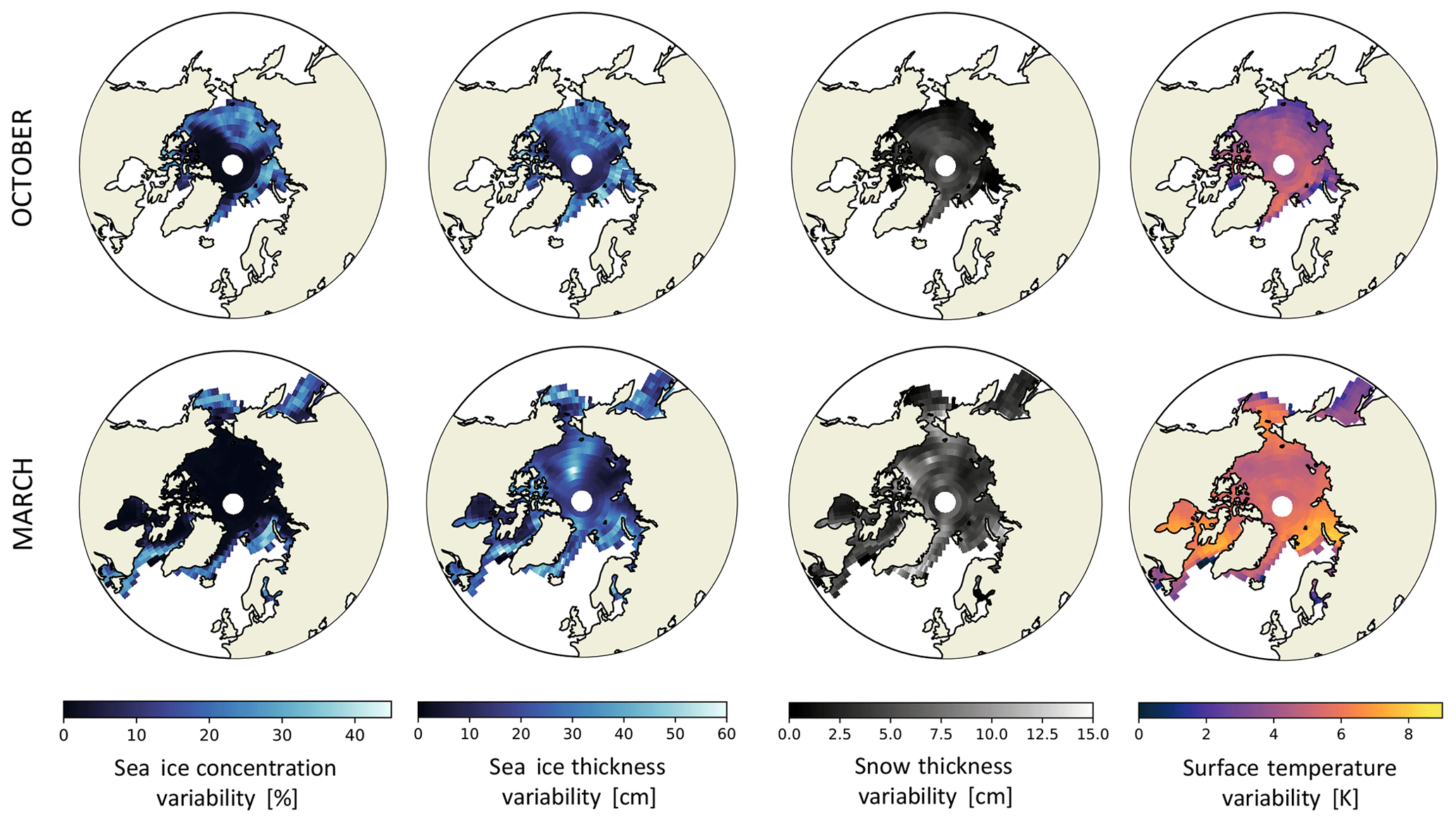
Figure B1Time mean of the standard deviation for each date over a sample of five years (2003 to 2008) for each variable and each grid cell. This standard deviation was the variability estimate used to modulate the input variables in the sensitivity studies of Sect. 4.3.2. These values are inferred from the SICCI2 assimilation run.
Primary data and scripts used in this study are archived by the Max Planck Institute for Meteorology and can be obtained by contacting publications@mpimet.mpg.de. The source code of ARC3O can be downloaded from https://github.com/ClimateClara/arc3o, Burgard, 2020.
CB, DN, and LTP developed the original idea of this paper. CB carried out all analyses and wrote the manuscript. CB, DN, LTP and RTT contributed to discussions.
The authors declare that they have no conflict of interest.
We thank Stefan Kern for constructive comments and discussions. We also thank two anonymous reviewers for very constructive and insightful comments.
This research has been funded by the European Space Agency (Sea Ice Climate Change Initiative Phase 2).
The article processing charges for this open-access
publication were covered by the Max Planck Society.
This paper was edited by Ludovic Brucker and reviewed by two anonymous referees.
Andersson, E., Pailleux, J., Thépaut, J.-N., Eyre, J., McNally, A., Kelly, G., and Courtier, P.: Use of cloud-cleared radiances in three/four-dimensional variational data assimilation, Q. J. Roy. Meteor. Soc., 120, 627–653, https://doi.org/10.1002/qj.49712051707, 1994. a
Bailey, D., DuVivier, A., Holland, M., Hunke, E., Lipscomb, B., Briegleb, B., Bitz, C., and Schramm, J.: CESM CICE5 Users Guide, Tech. rep., 2018. a
Balmaseda, M., Mogensen, K., and Weaver, A.: Evaluation of the ECMWF ocean reanalysis system ORAS4, Q. J. Roy. Meteor. Soc., 139, 1132–1161, https://doi.org/10.1002/qj.2063, 2013. a
Barber, D., Fung, A., Grenfell, T., Nghiem, S., Onstott, R., Lytle, V., Perovich, D., and Gow, A.: The role of snow on microwave emission and scattering over first-year sea ice, IEEE T. Geosci. Remote, 36, 1750–1763, https://doi.org/10.1109/36.718643, 1998. a
Boisvert, L., Webster, M., Petty, A., Markus, T., Bromwich, D., and Cullather, R.: Intercomparison of Precipitation Estimates over the Arctic Ocean and Its Peripheral Seas from Reanalyses, J. Climate, 31, 8441–8462, https://doi.org/10.1175/JCLI-D-18-0125.1, 2018. a
Brodzik, M., Long, D., Hardman, M., Paget, A., and Armstrong, R.: MEaSUREs Calibrated Enhanced-Resolution Passive Microwave Daily EASE-Grid 2.0 Brightness Temperature ESDR, Version 1, https://doi.org/10.5067/MEASURES/CRYOSPHERE/NSIDC-0630.001, 2016 (updated 2018). a
Bunzel, F., Notz, D., Baehr, J., Müller, W., and Fröhlich, K.: Seasonal climate forecasts significantly affected by observational uncertainty of Arctic sea ice concentration, Geophys. Res. Lett., 43, 852–859, https://doi.org/10.1002/2015GL066928, 2016. a, b, c, d
Burgard, C.: ARC3O, GitHub repository, available at: https://github.com/ClimateClara/arc3o, last access: July 2020. a
Burgard, C., Notz, D., Pedersen, L. T., and Tonboe, R. T.: The Arctic Ocean Observation Operator for 6.9 GHz (ARC3O) – Part 1: How to obtain sea ice brightness temperatures at 6.9 GHz from climate model output, The Cryosphere, 14, 2369–2386, https://doi.org/10.5194/tc-14-2369-2020, 2020. a, b, c, d, e, f, g, h, i, j, k, l, m, n
Cavalieri, D., Burns, B., and Onstott, R.: Investigation of the effects of summer melt on the calculation of sea ice concentration using active and passive microwave data, J. Geophys. Res.-Oceans, 95, 5359–5369, https://doi.org/10.1029/JC095iC04p05359, 1990. a
Cavalieri, D. J., Parkinson, C., Gloersen, P., and Zwally, H.: Sea ice concentrations from Nimbus-7 SMMR and DMSP SSM/I-SSMIS passive microwave data, version 1, https://doi.org/10.5067/8GQ8LZQVL0VL, 1996. a
Chang, T. and Gloersen, P.: Microwave Emission from dry and wet snow, in: Operational Applications of Satellite Snowcover Observations, edited by: Rango, A., chap. 27, NASA, 399–407, 1975. a
Comiso, J.: Bootstrap sea ice concentrations from Nimbus-7 SMMR and DMSP SSM/I-SSMIS, version 2, https://doi.org/10.5067/J6JQLS9EJ5HU, 2000. a
Comiso, J. and Kwok, R.: Surface and radiative characteristics of the summer Arctic sea ice cover from multisensor satellite observations, J. Geophys. Res.-Oceans, 101, 28397–28416, https://doi.org/10.1029/96JC02816, 1996. a, b
Comiso, J., Cavalieri, D., Parkinson, C., and Gloersen, P.: Passive Microwave Algorithms for Sea Ice Concentration: A Comparison of Two Techniques, Remote Sens. Environ., 60, 357–384, https://doi.org/10.1016/S0034-4257(96)00220-9, 1997. a
Dee, D., Uppala, S., Simmons, A., Berrisford, P., Poli, P., Kobayashi, S., Andrae, U., Balmaseda, M., Balsamo, G., Bauer, P., Bechtold, P., Beljaars, A., van de Berg, L., Bidlot, J., Bormann, N., Delsol, C., Dragani, R., Fuentes, M., Geer, A., Haimberger, L., Healy, S., Hersbach, H., Holm, E., Isaksen, L., Kållberg, P., Köhler, M., Matricardi, M., McNally, A., Monge-Sanz, B., Morcrette, J.-J., Park, B.-K., Peubey, C., de Rosnay, P., Tavolato, C., Thébaut, J.-N., and Vitart, F.: The ERA-Interim reanalysis: configuration and performance of the data assimilation system, Q. J. Roy. Meteor. Soc., 137, 553–597, https://doi.org/10.1002/qj.828, 2011. a
Evensen, G.: Sequential data assimilation with a nonlinear quasi-geostrophic model using Monte Carlo methods to forecast error statistics, J. Geophys. Res.-Oceans, 99, 10143–10162, https://doi.org/10.1029/94JC00572, 1994. a
Eyring, V., Bony, S., Meehl, G. A., Senior, C. A., Stevens, B., Stouffer, R. J., and Taylor, K. E.: Overview of the Coupled Model Intercomparison Project Phase 6 (CMIP6) experimental design and organization, Geosci. Model Dev., 9, 1937–1958, https://doi.org/10.5194/gmd-9-1937-2016, 2016. a
Eyring, V., Cox, P., Flato, G., Gleckler, P., Abramowitz, G., Caldwell, P., Collins, W., Gier, B., Hall, A., Hoffman, F., Hurtt, G., Jahn, A., Jones, C., Klein, S., Krasting, J., Kwiatkowski, L., Lorenz, R., Maloney, E., Meehl, G., Pendergrass, A., Pincus, R., Ruane, A., Russell, J., Sanderson, B., Santer, B., Sherwood, S., Simpson, I., Stouffer, R., and Williamson, M.: Taking climate model evaluation to the next level, Nat. Clim. Change, 9, 102–110, https://doi.org/10.1038/s41558-018-0355-y, 2019. a
Fetterer, F. and Untersteiner, N.: Observations of melt ponds on Arctic sea ice, J. Geophys. Res.-Oceans, 103, 24821–24835, https://doi.org/10.1029/98JC02034, 1998. a
Flato, G., Marotzke, J., Abiodun, B., Braconnot, P., Chou, S., Collins, W., Cox, P., Driouech, F., Emori, S., Eyring, V., Forest, C., Gleckler, P., Guilyardi, E., Jakob, C., Kattsov, V., Reason, C., and Rummukainen, M.: Evaluation of Climate Models, book section 9, Cambridge University Press, Cambridge, United Kingdom and New York, NY, USA, 741–866, https://doi.org/10.1017/CBO9781107415324.020, 2013. a
Giorgetta, M., Roeckner, E., Mauritsen, T., Bader, J., Crueger, T., Esch, M., Rast, S., Kornblueh, L., Schmidt, H., Kinne, S., Hohenegger, C., Möbis, B., Krismer, T., Wieners, K., and Stevens, B.: The atmospheric general circulation model ECHAM6: Model description, Tech. Rep. Reports on Earth System Science, 135/2013, Max Planck Institute for Meteorology, 2013. a, b
Griewank, P. J. and Notz, D.: A 1-D modelling study of Arctic sea-ice salinity, The Cryosphere, 9, 305–329, https://doi.org/10.5194/tc-9-305-2015, 2015. a
Hallikainen, M. and Winebrenner, D.: The Physical Basis for Sea Ice Remote Sensing, in: Microwave Remote Sensing of Sea Ice, edited by: Carsey, F., chap. 4, American Geophysical Union, 29–46, 1992. a
Hallikainen, M., Ulaby, F., and Abdelrazik, M.: Dielectric properties of snow in the 3 to 37 GHz range, IEEE T. Antenn. Propag., 34, 1329–1340, https://doi.org/10.1109/TAP.1986.1143757, 1986. a
Hibler, W.: A Dynamic Thermodynamic Sea Ice Model, J. Phys. Oceanogr., 9, 815–846, 1979. a
Hunt, B., Kostelich, E., and Szunyogh, I.: Efficient data assimilation for spatiotemporal chaos: A local ensemble transform Kalman filter, Physica D, 230, 112–126, https://doi.org/10.1016/j.physd.2006.11.008, 2007. a
Istomina, L., Heygster, G., Huntemann, M., Marks, H., Melsheimer, C., Zege, E., Malinka, A., Prikhach, A., and Katsev, I.: Melt pond fraction and spectral sea ice albedo retrieval from MERIS data – Part 2: Case studies and trends of sea ice albedo and melt ponds in the Arctic for years 2002–2011, The Cryosphere, 9, 1567–1578, https://doi.org/10.5194/tc-9-1567-2015, 2015a. a, b, c
Istomina, L., Heygster, G., Huntemann, M., Schwarz, P., Birnbaum, G., Scharien, R., Polashenski, C., Perovich, D., Zege, E., Malinka, A., Prikhach, A., and Katsev, I.: Melt pond fraction and spectral sea ice albedo retrieval from MERIS data – Part 1: Validation against in situ, aerial, and ship cruise data, The Cryosphere, 9, 1551–1566, https://doi.org/10.5194/tc-9-1551-2015, 2015b. a, b
Ivanova, N., Johannessen, O. M., Pedersen, L. T., and Tonboe, R. T.: Retrieval of Arctic Sea Ice Parameters by Satellite Passive Microwave Sensors: A Comparison of Eleven Sea Ice Concentration Algorithms, IEEE T. Geosci. Remote, 52, 7233–7246, https://doi.org/10.1109/TGRS.2014.2310136, 2014. a, b, c
Ivanova, N., Pedersen, L. T., Tonboe, R. T., Kern, S., Heygster, G., Lavergne, T., Sørensen, A., Saldo, R., Dybkjær, G., Brucker, L., and Shokr, M.: Inter-comparison and evaluation of sea ice algorithms: towards further identification of challenges and optimal approach using passive microwave observations, The Cryosphere, 9, 1797–1817, https://doi.org/10.5194/tc-9-1797-2015, 2015. a, b, c, d
Jakobson, E., Vihma, T., Keernik, H., and Jaagus, J.: Validation of atmospheric reanalyses over the central Arctic Ocean, Geophys. Res. Lett., 39, L10802, https://doi.org/10.1029/2012GL051591, 2012. a
Jungclaus, J., Fischer, N., Haak, H., Lohmann, K., Marotzke, J., Matei, D., Mikolajewicz, U., Notz, D., and von Storch, J.: Characteristics of the ocean simulations in the Max Planck Institute Ocean Model (MPIOM) the ocean component of the MPI-Earth system model, J. Adv. Model Earth Sy., 5, 422–446, https://doi.org/10.1002/jame.20023, 2013. a, b
Kern, S., Rösel, A., Pedersen, L. T., Ivanova, N., Saldo, R., and Tonboe, R. T.: The impact of melt ponds on summertime microwave brightness temperatures and sea-ice concentrations, The Cryosphere, 10, 2217–2239, https://doi.org/10.5194/tc-10-2217-2016, 2016. a, b, c
Kern, S., Lavergne, T., Notz, D., Pedersen, L. T., Tonboe, R. T., Saldo, R., and Sørensen, A. M.: Satellite passive microwave sea-ice concentration data set intercomparison: closed ice and ship-based observations, The Cryosphere, 13, 3261–3307, https://doi.org/10.5194/tc-13-3261-2019, 2019. a, b, c
Lavergne, T., Sørensen, A. M., Kern, S., Tonboe, R., Notz, D., Aaboe, S., Bell, L., Dybkjær, G., Eastwood, S., Gabarro, C., Heygster, G., Killie, M. A., Brandt Kreiner, M., Lavelle, J., Saldo, R., Sandven, S., and Pedersen, L. T.: Version 2 of the EUMETSAT OSI SAF and ESA CCI sea-ice concentration climate data records, The Cryosphere, 13, 49–78, https://doi.org/10.5194/tc-13-49-2019, 2019. a, b, c
Lee, S.-M., Sohn, B.-J., and Shi, H.: Impact of ice surface and volume scatterings on the microwave sea ice apparent emissivity, J. Geophys. Res.-Atmos., 123, 9220–9237, https://doi.org/10.1029/2018JD028688, 2018. a
Lindsay, R., Wensnahan, M., Schweiger, A., and Zhang, J.: Evaluation of Seven Different Atmospheric Reanalysis Products in the Arctic, J. Climate, 27, 2588–2606, https://doi.org/10.1175/JCLI-D-13-00014.1, 2014. a, b
Meier, W. and Notz, D.: A note on the accuracy and reliability of satellite-derived passive microwave estimates of sea-ice extent, CliC Arctic sea ice working group consensus document, World Climate Research Program, 2010. a
Nandan, V., Geldsetzer, T., Yackel, J., Mahmud, M., Scharien, R., Howell, S., King, J., Ricker, R., and Else, B.: Effect of Snow Salinity on CryoSat-2 Arctic First-Year Sea Ice Freeboard Measurements, Geophys. Res. Lett., 44, 419–426, https://doi.org/10.1002/2017GL074506, 2017. a
NASDA: AMSR-E Data Users Handbook, Tech. Rep. NCX-030021, Earth Observation Center, National Space Development Agency of Japan, Japan, 2003. a
Niederdrenk, A. and Notz, D.: Arctic sea ice in a 1.5 ∘C warmer world, Geophys. Res. Lett., 45, 1963–1971, https://doi.org/10.1002/2017GL076159, 2018. a
Notz, D.: Thermodynamic and Fluid-Dynamical Processes in Sea Ice, PhD thesis, University of Cambridge, 2005. a, b
Notz, D. and Stroeve, J.: Observed Arctic sea-ice loss directly follows anthropogenic CO2 emission, Science, 354, 767–750, https://doi.org/10.1126/science.aag2345, 2016. a
Notz, D., Haumann, A., Haak, H., and Marotzke, J.: Arctic sea-ice evolution as modeled by Max Planck Institute for Meteorology's Earth system model, J. Adv. Model Earth Sy., 5, 173–194, https://doi.org/10.1002/jame.20016, 2013. a, b, c
Pedersen, L., Saldo, R., Ivanova, N., Kern, S., Heygster, G., Tonboe, R., Huntemann, M., Ozsoy, B., Ardhuin, F., and Kaleschke, L.: Reference dataset for sea ice concentration, Figshare, https://doi.org/10.6084/m9.figshare.6626549.v6, 2018. a
Pounder, E.: The Physics of Ice, Elsevier, 1st Edn., 1965. a
Richter, F., Drusch, M., Kaleschke, L., Maaß, N., Tian-Kunze, X., and Mecklenburg, S.: Arctic sea ice signatures: L-band brightness temperature sensitivity comparison using two radiation transfer models, The Cryosphere, 12, 921–933, https://doi.org/10.5194/tc-12-921-2018, 2018. a, b, c
Ricker, R., Hendricks, S., Kaleschke, L., Tian-Kunze, X., King, J., and Haas, C.: A weekly Arctic sea-ice thickness data record from merged CryoSat-2 and SMOS satellite data, Cryosphere, 11, 1607–1623, https://doi.org/10.5194/tc-11-1607-2017, 2017. a
Roeckner, E., Mauritsen, T., Esch, M., and Brokopf, R.: Impact of melt ponds on Arctic sea ice in past and future climates as simulated by MPI-ESM, J. Adv. Model Earth Sy., 4, https://doi.org/10.1029/2012MS000157, 2012. a, b
Rösel, A., Kaleschke, L., and Birnbaum, G.: Melt ponds on Arctic sea ice determined from MODIS satellite data using an artificial neural network, The Cryosphere, 6, 431–446, https://doi.org/10.5194/tc-6-431-2012, 2012a. a, b, c
Rösel, A., Kaleschke, L., and Kern, S.: Influence of melt ponds on microwave sensors' sea ice concentration retrieval algorithms, 2012 IEEE International Geoscience and Remote Sensing Symposium, 3261–3264, https://doi.org/10.1109/IGARSS.2012.6350608, 2012b. a
Scott, K. A., Buehner, M., Caya, A., and Carrieres, T.: Direct Assimilation of AMSR-E Brightness Temperatures for Estimating Sea Ice Concentration, Mon. Weather Rev., 140, 997–1013, https://doi.org/10.1175/MWR-D-11-00014.1, 2012. a
Shokr, M. and Sinha, N.: Remote Sensing Principles Relevant to Sea Ice, in: Sea Ice: Physics and Remote Sensing, Geophysical Monograph 209, First Edn., American Geophysical Union, chap. 7, John Wiley & Sons, Inc., 271–335, 2015. a, b, c
Stevens, B., Giorgetta, M., Esch, M., Mauritsen, T., Crueger, T., Rast, S., Salzmann, M., Schmidt, H., Bader, J., Block, K., Brokopf, R., Fast, I., Kinne, S., Kornblueh, L., Lohmann, U., Pincus, R., Reichler, T., and Roeckner, E.: Atmospheric component of the MPI-M Earth System Model: ECHAM6, J. Adv. Model Earth Sy., 5, 146–172, https://doi.org/10.1002/jame.20015, 2013. a
Swift, C. and Cavalieri, D.: Passive microwave remote sensing for sea ice research, Eos T. Am. Geophys. Un., 66, 1210–1212, https://doi.org/10.1029/EO066i049p01210, 1985. a
Talagrand, O. and Courtier, P.: Variational Assimilation of Meteorological Observations With the Adjoint Vorticity Equation. I: Theory, Q. J. Roy. Meteor. Soc., 113, 1311–1328, https://doi.org/10.1002/qj.49711347812, 1987. a
Taylor, K., Stouffer, R., and Meehl, G.: An Overview of CMIP5 and the Experiment Design, B. Am. Meteorol. Soc., 93, 485–498, 2012. a
Terasaki, K. and Miyoshi, T.: Assimilating AMSU-A Radiances with the NICAM-LETKF, J. Meteorol. Soc. Jpn. Ser. II, 95, 433–446, https://doi.org/10.2151/jmsj.2017-028, 2017. a
Tietsche, S., Notz, D., Jungclaus, J. H., and Marotzke, J.: Assimilation of sea-ice concentration in a global climate model – physical and statistical aspects, Ocean Sci., 9, 19–36, https://doi.org/10.5194/os-9-19-2013, 2013. a
Tonboe, R.: The simulated sea ice thermal microwave emission at window and sounding frequencies, Tellus, 62A, 333–344, https://doi.org/10.1111/j.1600-0870.2010.00434.x, 2010. a, b, c
Tonboe, R., Andersen, S., Toudal, L., and Heygster, G.: Sea ice emission modelling, in: Thermal Microwave Radiation - Applications for Remote Sensing, edited: by Mätzler, C., Rosenkranz, P., Battaglia, A., and Wigneron, J., IET Electromagnetic Waves Series 52, 382–400, 2006. a
Tonboe, R. T., Eastwood, S., Lavergne, T., Sørensen, A. M., Rathmann, N., Dybkjær, G., Pedersen, L. T., Høyer, J. L., and Kern, S.: The EUMETSAT sea ice concentration climate data record, The Cryosphere, 10, 2275–2290, https://doi.org/10.5194/tc-10-2275-2016, 2016. a
Ulaby, F., Moore, R., and Fung, A.: Passive microwave sensing of the ocean, in: Microwave Remote Sensing, Active and Passive Volume III, From Theory to Applications, chap. 18, Artech House, Inc., 1412–1521, 1986. a, b, c
Vancoppenolle, M., Fichefet, T., Goosse, H., Bouillon, S., Madec, G., and Morales Maqueda, M.: Simulating the mass balance and salinity of Arctic and Antarctic sea ice. 1. Model description and validation, Ocean Model., 27, 33–53, https://doi.org/10.1016/j.ocemod.2008.10.005, 2009. a
Wentz, F. and Meissner, T.: Algorithm theoretical basis document (atbd), version 2, Tech. Rep. AMSR Ocean Algorithm, RSS Tech. Proposal 121599A-1, Remote Sensing Systems, Santa Rosa, CA, 2000. a, b
Wiesmann, A. and Mätzler, C.: Microwave emission model of layered snowpacks, Remote Sens. Environ., 70, 307–316, 1999. a
- Abstract
- Introduction
- The Max Planck Institute Earth System Model
- The Arctic Ocean Observation Operator ARC3O
- Evaluation of ARC3O
- Conclusions
- Outlook
- Appendix A: Tuning of the temperature profiles
- Appendix B: Variability in climate parameters
- Code and data availability
- Author contributions
- Competing interests
- Acknowledgements
- Financial support
- Review statement
- References