the Creative Commons Attribution 4.0 License.
the Creative Commons Attribution 4.0 License.
 | 21 Jul 2020
Results of the third Marine Ice Sheet Model Intercomparison Project (MISMIP+)
Stephen L. Cornford
Helene Seroussi
Xylar S. Asay-Davis
G. Hilmar Gudmundsson
Rob Arthern
Chris Borstad
Julia Christmann
Thiago Dias dos Santos
Johannes Feldmann
Daniel Goldberg
Matthew J. Hoffman
Angelika Humbert
Thomas Kleiner
Gunter Leguy
William H. Lipscomb
Nacho Merino
Gaël Durand
Mathieu Morlighem
David Pollard
Martin Rückamp
C. Rosie Williams
Hongju Yu
We present the result of the third Marine Ice Sheet Model Intercomparison Project, MISMIP+. MISMIP+ is intended to be a benchmark for ice-flow models which include fast sliding marine ice streams and floating ice shelves and in particular a treatment of viscous stress that is sufficient to model buttressing, where upstream ice flow is restrained by a downstream ice shelf. A set of idealized experiments first tests that models are able to maintain a steady state with the grounding line located on a retrograde slope due to buttressing and then explore scenarios where a reduction in that buttressing causes ice stream acceleration, thinning, and grounding line retreat. The majority of participating models passed the first test and then produced similar responses to the loss of buttressing. We find that the most important distinction between models in this particular type of simulation is in the treatment of sliding at the bed, with other distinctions – notably the difference between the simpler and more complete treatments of englacial stress but also the differences between numerical methods – taking a secondary role.
- Article
(4294 KB) - Full-text XML
- BibTeX
- EndNote


A number of ice-flow models have been developed in the last decade that simulate fast-flowing ice streams and ice shelves as well as larger, slower-moving ice masses. The key difference between this generation of models and the previous generation is their choice of viscous stress balance equations. All ice sheet models are based upon Stokes flow or, more commonly, one of several approximations to Stokes flow (Hindmarsh, 2004; Greve and Blatter, 2009; Pattyn and Durand, 2013). Models designed to simulate the creeping flow of continental ice sheets over glacial cycles are typically based on the shallow ice approximation (SIA), which considers only vertical shear stresses, while more complete approximations are needed for ice shelves and ice streams. The simplest model that can be applied is the shallow-shelf/shelfy-stream approximation (MacAyeal, 1989), which includes horizontal normal and shear stresses and requires the solution of vertically integrated, two-dimensional stress balance equations. More complete models include the L1Lx class of vertically integrated models (Hindmarsh, 2004; Schoof and Hindmarsh, 2010), which resemble the SSA in many respects; the higher-order (HO) models (Pattyn, 2003), which require the solution of simplified three-dimensional stress equations; and the complete Stokes models that include all viscous stresses (Le Meur et al., 2004).
There have been several community exercises comparing ice sheet models where ice stream and shelf dynamics are important. These can be divided into two types: exercises involving real-world ice flows, perhaps forced with climate inputs from sophisticated atmosphere and ocean models (Seroussi et al., 2019; Goelzer et al., 2018), and exercises involving idealized settings with simple forcings. This paper describes the results of an idealized exercise, which can be regarded as sequential to three previous exercises. The Ice Sheet Model Intercomparison Project for Higher-Order Model (ISMIP-HOM, Pattyn et al., 2008) quantified the differences between SIA, SSA, higher-order, and full-Stokes models in time independent settings with periodic bedrock topography and slipperiness. The first Marine Ice Sheet Model Intercomparison Project (MISMIP, Pattyn et al. (2012)) considered a time-dependent but laterally unvarying problem and highlighted the technical challenges faced by numerical models of an ice stream with both grounded and floating portions, that is, with a grounding line. Many models failed to reproduce theoretically well understood properties of such systems. Notably, that a laterally unvarying ice stream on a bedrock that slopes monotonically down in the direction of flow has a single equilibrium state where ice flux across the grounding line matches the total accumulation upstream. The second Marine Ice Sheet Model Intercomparison Project (MISMIP3D, Pattyn et al., 2013) extended a subset of the MISMIP experiments to include perturbations with some lateral variation and once again demonstrated that many models of the time did not exhibit the expected unique equilibrium state. It did not, however, feature strong buttressing of the kind that is important in Antarctic ice shelf and ice stream systems. Recent real-world cases include applications to Pine Island Glacier (Joughin et al., 2019) and Thwaites Glacier (Yu et al., 2018) in western Antarctica and in Antarctica as a whole (Gudmundsson et al., 2019; Martin et al., 2019).
MISMIP+ explores the ability of ice sheet models to simulate coupled ice sheet and ice shelf systems where the ice shelf strongly buttresses the flow upstream and to respond to a loss of buttressing caused by ice shelf ablation. All of the experiments are based around an idealized ice stream, adapted from Gudmundsson (2013), with ice sliding into an ice shelf along a bedrock trough with steep walls (Sect. 2.1). Part of the bedrock trough is retrograde – it slopes upward in the direction of flow – and key model parameters are chosen so that, in the absence of sub-ice-shelf melting, models should form a stable equilibrium state with the grounding line crossing the center of the channel on this retrograde slope. The equilibrium state is only stable because of lateral variation in the flow field: it is well known that without such stresses stable steady states form only when the grounding line lies on a prograde slope (Schoof, 2007). The experimental design was stated in Asay-Davis et al. (2016); in this paper we recap the design for convenience and report the results from 15 distinct participants, several of whom carried out the experiments with multiple model configurations.
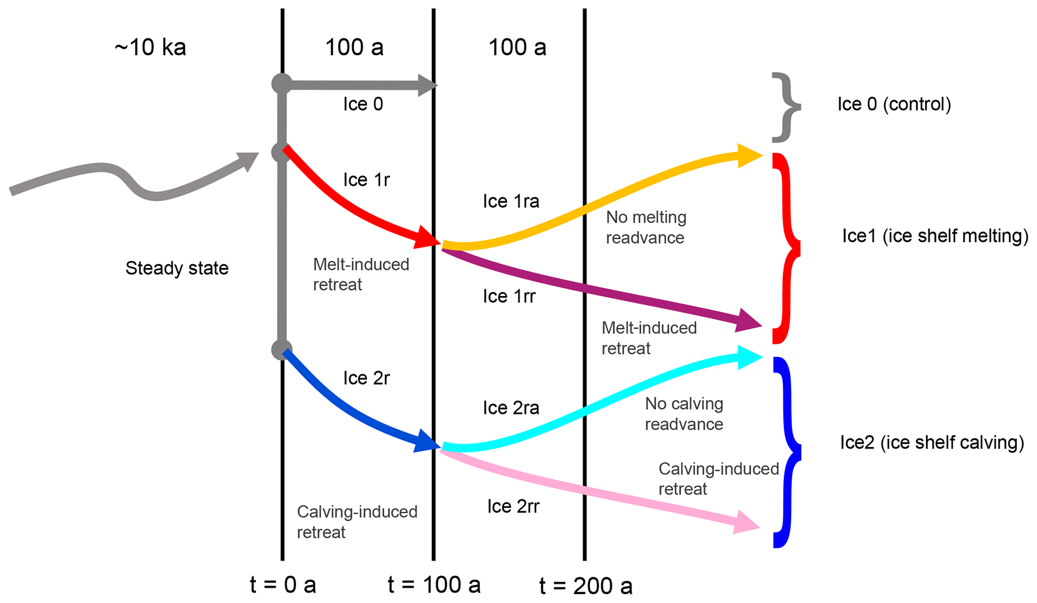
Figure 1Relationship between the MISMIP+ Ice0, Ice1, and Ice2 experiments. An upward sloping curve indicates an advancing grounding line, a downward sloping curve a retreating grounding line. All three experiments start from a common steady state. The Ice0 experiment provides a control for the Ice1 and Ice2 experiments, which induce retreat with ice shelf melting or calving respectively for 100 a. Later stages of the experiments remove or continue the melting or calving.
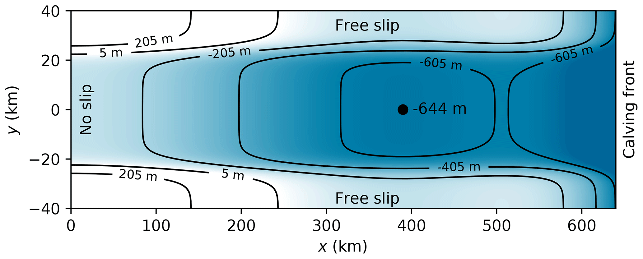
Figure 2MISMIP+ domain showing bedrock elevation zb(x,y) and boundary types. The spot height (−644 m) indicates the beginning of a retrograde slope in the center of the channel.
Three groups of experiments (Fig. 1) were carried out. The Ice0 experiments (Sect. 2.5) were designed to show that models were close to steady state at the start of the experiments (time t=0). The Ice1 experiments (Sect. 2.6) saw the ice shelves subjected to ablation at the base of the ice, with a simple formula intended to resemble the gross features of melt rates computed by ocean circulation models, with maximum melt rates close to (but not at) the grounding line. Ice shelf ablation also drives the Ice2 experiments (Sect. 2.7), but in this case the imposed ablation is concentrated at the calving front and does not evolve over time.
2.1 Geometry
The MISMIP+ ice stream is set in a rectangular domain, spanning 640 km in the x direction and 80 km in the y direction. Ice flows in a direction roughly parallel to the x axis from x=0 toward x=640 km, so we will refer to x as the along-flow direction and y as the lateral- or across-flow direction. A no-slip boundary applies at x=0 and free-slip boundaries apply at both lateral boundaries, while calving front boundary conditions apply at x=640 km. This choice of boundary conditions, together with the bedrock geometry and mass sources and sinks, results in solutions that have mirror symmetry about the lateral center of the ice stream. For that reason, some participants chose to run their experiments in only one half of the domain, a perfectly acceptable practice for the MISMIP+ and MISMP3d (Pattyn et al., 2013) experiments, though not the related ISOMIP+ and MISOMIP experiments (Asay-Davis et al., 2016), where ocean circulation results in nonaxisymmetric melt rates. For convenience in this paper, we define y such that km, in contrast with Asay-Davis et al. (2016), so that the axis of symmetry is the x axis.
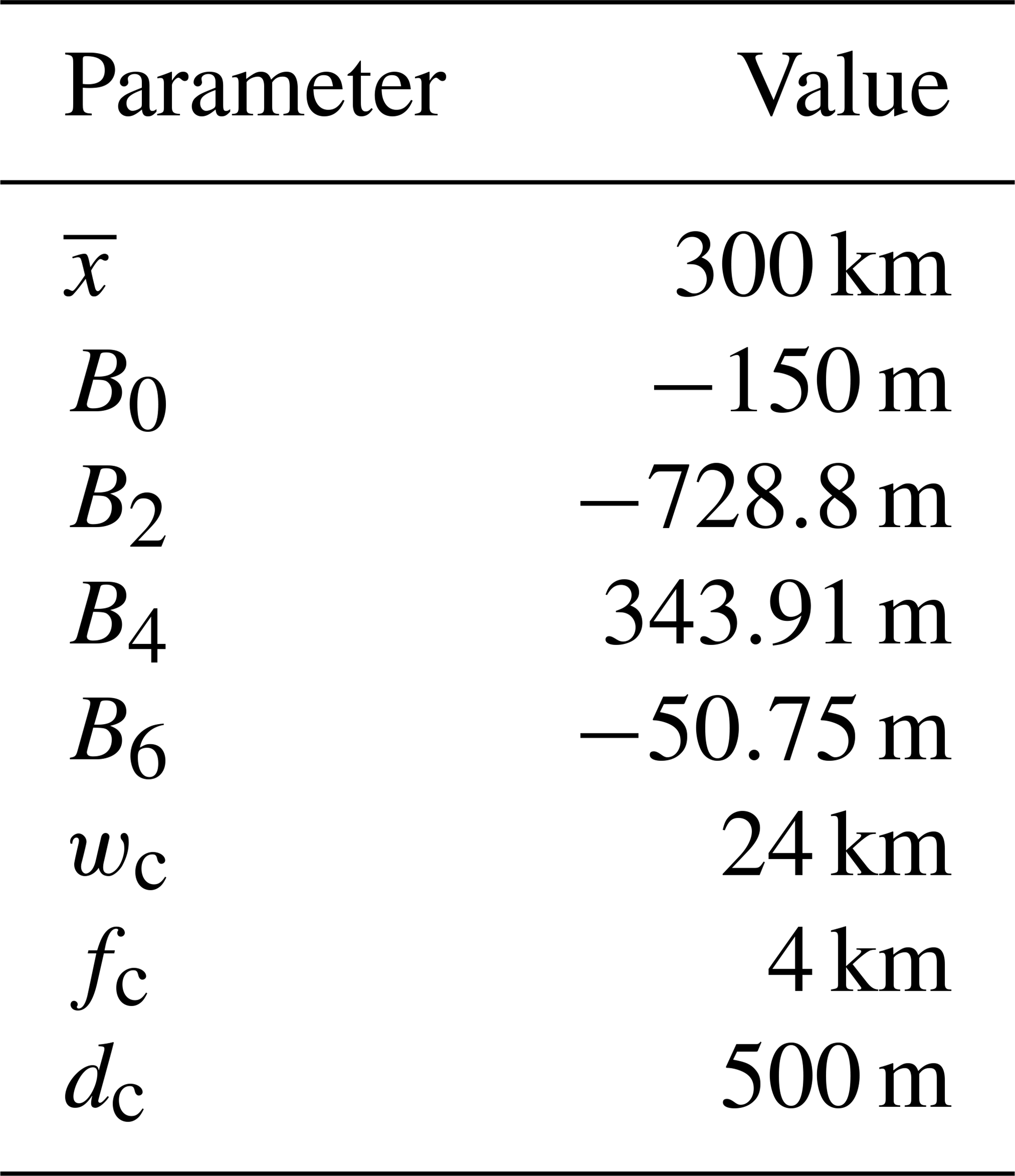
The bedrock elevation zb, measured in meters, is given by
where
and
with the parameters value given in Table 1. Figure 2 illustrates the main features of Eq. (1): a steep-walled channel around 48 km wide running parallel to the x axis, and a ridge around x=505 km. Ice flows from the divide at x=0 toward the calving front at x=640 km, so that portion of the ridge between x=390 km and the summit at x=505 km is retrograde: it slopes upward in the direction of ice flow.
2.2 Initial state
Participants were asked to compute a steady state given the bedrock geometry and boundary conditions above, a constant rate of accumulation a=0.3 m a−1, and no melting at the ice shelf base. No particular method was prescribed. Participants simply needed to show that their initial state was sufficiently close to equilibrium that model drift in experiment Ice0 was small compared to the response to the perturbations of the Ice1 and Ice2 experiments. An obvious if time-consuming method is to carry out a spin-up, evolving the ice sheet from some simple initial state over tens of thousands of model years. Alternatives include taking a steady state from some simpler model and relaxing it over a shorter period of time – a method that might be useful, for example, when working with full-Stokes models.
One point of departure from the previous MISMIP designs is the specification of the initial-steady-state grounding line position, rather than a full set of model parameters. Participants were asked to produce a steady state where the grounding line crossed the center of the channel (y=0) at a point km, that is, on the retrograde slope. In order to meet this requirement, participants were free to set any value at all for the rate factor A, which affects stresses within the ice (Sect. 2.3), and for the basal friction coefficient β2, which affects stresses at the ice base (Sect. 2.4). This is a key part of the design for two reasons. First, we wanted all models to begin with their grounding line in steady state on the partly retrograde bed to test that all models could achieve this basic result. Second, we wanted to more closely emulate real-world applications of ice sheet models, where the present day geometry of the ice sheet might be well known, but parameters such as A and β2 are unknown and are found by some kind of calibration.
2.3 Englacial stresses
Participants were permitted to choose any approximation at all for the englacial stresses. That said, the shallow-shelf/shelfy-stream approximation (SSA, MacAyeal, 1989) is the simplest approximation that includes the horizontal normal and shear stresses that describe the coupling between floating and grounded ice, so that in particular we did not expect submissions based solely on the shallow ice approximation (SIA). See, for example, Hindmarsh (2004); Greve and Blatter (2009) for a discussion of stress approximations. Whichever approximation was chosen, it was expected to involve Glen's flow law. In the general case, strain rate components Dij and deviatoric stress components τij satisfy
where n=3 and . Participants were free to chose any constant A in order to realize a steady state within the specified tolerance, though a suggested value was given: Pa−3 a−1 ( Pa−3 s−1).
2.4 Basal friction
Participants submitted results from simulations carried out with one or more of three basal friction laws. All three ensure that the basal friction τb=0 for floating ice, but differ in their approach to ice close to flotation, where the effective pressure at the base, N, is low. The simplest of the three is based on the Weertman (1957) rule for sliding over hard beds, with
where u is the horizontal ice velocity at the bed.
Although well known, the Weertman (1957) sliding law is certainly not the final word on glacier sliding (Fowler, 2010; Joughin et al., 2019). Taking a pragmatic (and model-centered) view, it may not be applicable close to the grounding line, where τb will be discontinuous. The two alternative rules considered here ensure that τb is continuous (but not differentiable)1. Schoof (2005) and, later, Leguy et al. (2014) considered the case of sliding with cavitation, over hard beds, leading to a rule,
which, among other features, ensures that does not exceed some fraction α2 of the effective pressure but can be approximated by the Weertman (1957) rule far from the grounding line where N is large. Tsai et al. (2015) considered a case where friction is due to either sliding over hard beds at high N and deforming beds when N is low. The resulting rule is
We refer to both modified rules as Coulomb-limited, because the Schoof (2005) and Tsai et al. (2015) rules both imply : in other words, that the magnitude of the basal friction cannot exceed that given by a Coulomb law,
where α2<1 is a coefficient of friction. Joughin et al. (2019) uses the term regularized Coulomb, reflecting another benefit of this class of rules: that they permit Coulomb sliding but do not insist upon it over the whole domain, which would be problematic for two reasons. The first problem is physical: across much of the ice sheet N ≳ 1 MPa, leading to a magnitude of friction larger than observed. The second problem is mathematical, or at least pragmatic: if does not increase with anywhere in the domain, then a Dirichlet condition for u must be imposed on at least some part of the horizontal boundary. The modified rules avoid both of these problems by reverting to the familiar Weertman (1957) rule of Eq. (3) where N is large (or ice flows slowly in the case of Joughin et al., 2019).
In all three cases participants were free to modify the parameter β2 in order to achieve the desired steady state: the suggested value was β2=104 Pa m a1∕3 (3.16×10⁶ Pa m s1∕3).
2.5 The Ice0 experiment
The Ice0 experiment is simply a test of the initial steady state. Simulations ran from t=0 a to t=100 a, with zero sub-ice-shelf melt and an upper surface accumulation rate a=0.3 m a−1. Since these are the melt and accumulation rates defining the the initial steady state, models should exhibit little or no variability during this process, or, if they do exhibit some variation, it should result in little long-term drift. That is, fluctuations in ice thickness were acceptable provided that the grounding line did not advance or retreat and the ice volume did not grow or shrink to any great extent compared to the other two experiments. Participants were free to produce the initial state by any method; the majority of participants chose to evolve their models with the stated parameters for ∼10 ka in order to approach steady state.
2.6 Oceanic forcing and the Ice1 experiments
The Ice1 experiments were intended to examine the response of models to intense ablation at the base of the ice shelf, with a spatial distribution reflecting the results of typical cavity circulation models (Asay-Davis et al., 2016). The melt rate, measured in m a−1, was
where zd is the ice shelf draft and zd−zb is the cavity thickness, both measured in meters. The resulting melt rate will generally increase with draft, reaching values of around 100 m a−1 when zd≈700 m, but will vanish at the grounding line where the cavity thickness is zero. In the Ice1r experiment, the melt rate was applied to floating ice over the course of 100 a, starting from the steady state at t=0. This results in the loss of much of the original ice shelf thickness over the course of the experiment and was expected to result in grounding line retreat, assuming that the ice shelf had a role in buttressing the ice upstream. The two follow-on experiments, Ice1rr and Ice1ra, were designed to start from the end of the Ice1 experiment at t=100 a and terminate at t=200 a. Ice1rr is simply a continuation of Ice1r, with the same melt rate applied, while Ice1ra imposes zero melt rate, allowing the ice shelf to thicken, so that the grounding line should readvance.
2.7 Calving and the Ice2 experiments
The Ice2 experiments follow the same basic structure as the Ice1 experiments but impose a different melt rate,
applied to ice shelf regions only. This choice of melt rate in Ice2 results in something like a large calving event, where a downstream portion of the ice shelf, amounting to around half the total area, is removed over a short period of time. The majority of the ice removed lies in a zone that provides little buttressing. By allowing a thick ice shelf to form in the wake of the retreating grounding line, the Ice2 experiments test a model's ability to form a new stable steady state with the grounding line on a retrograde slope. They also test the numerical implementation of the model, because there is often an abrupt increase in melt rate immediately downstream from some portions of the grounding line, in contrast to the smooth increase in melt rates seen in the Ice1 experiments.
The participating models cover the same variety of englacial stress approximations as the earlier MISMIP (Pattyn et al., 2012) and MISMIP3d (Pattyn et al., 2013) exercises, with each model including some approximation of the horizontal normal and shear stress (membrane stress). The most complete models make use of the full-Stokes equations, but the computational expense entailed by solving the full 3D stress balance equation limits both the number of participants able to run such a model and the number of submissions from those participants, so that there are only two full-Stokes submissions. The most common class of model is based upon a 2D, vertically integrated hydrostatic stress balance equation, either through the shallow-shelf/shelfy-stream approximation (SSA), which neglects shear strains Dxz and Dyz above the bed, or an approximation that assumes a simple form for Dxz and Dyz, for example, the models of Schoof and Hindmarsh (2010) and Goldberg (2011). We will follow Pattyn and Durand (2013) in labeling this second class of vertically integrated model “L1Lx”. Intermediate in complexity are the higher-order (HO) or first-order models, which include the hydrostatic Blatter–Pattyn models. HO models exploit the low aspect ratio of ice sheets to reduce the four 3D Stokes equations to a pair of 3D equations in the horizontal velocity components. Finally, the HySSA models solve the 2D SSA stress balance equation but adapt that analytic expression (Schoof, 2007) derived for flow-line models with no buttressing to the general case by means of a heuristic buttressing factor: such models were able to produce results in earlier exercises that, in contrast to all other types, did not depend strongly on mesh resolution.
All of the participating models construct and solve their stress balance and mass transport equations though a limited choice of methods. There are several finite-volume methods and finite-difference methods based on rectangular meshes, extruded vertically, and several finite-element methods based on unstructured triangular meshes, also extruded vertically. One model (MALI) takes a mixed approach, combining a finite-element discretization of the stress balance equation with a finite-volume discretization of the mass transport equation. The majority of finite-volume and finite-difference methods employ spatially uniform meshes, with two exceptions: WAVI employs a wavelet-based adaptive grid to reduce the computational expense in solving the stress balance equation, while BISICLES makes use of a time-evolving adaptive block structured mesh in both the stress balance and mass transport equations. The finite-element methods tend to employ spatially nonuniform meshes that do not change over the course of the simulation, with the exception of two of the several Ice Sheet System Model (ISSM) submissions, which update their meshes over time.
Models differ in their discretization of the stress balance equations in the region close to the grounding line. One common class of techniques is the modification of the discretized basal friction term around the grounding line. These techniques have been given at least two different names in the literature – grounding line parameterization (Gladstone et al., 2010; Leguy et al., 2014) and sub-element parameterization (Seroussi et al., 2014b) – but they all represent a similar approach. We will use the terms preferred by the individual model authors when referring to their submissions. The simplest type constructs a piecewise linear approximation to the thickness above flotation (h−hf) and uses that to evaluate a weight, , associated with each grid cell or element that reduces the discrete approximation to the friction term accordingly. None of these schemes introduce additional degrees of freedom, and they also have the same order of accuracy with respect to mesh resolution, O(Δx), as the unmodified scheme. Nonetheless, they have been seen to improve accuracy for a given mesh resolution in several cases (Feldmann et al., 2014; Seroussi et al., 2014a). A related – but more controversial (Seroussi and Morlighem, 2018) – modification to standard methods applies a similar weighting to the basal melt rate term in the mass balance equation. Several participants employed such a modification in these exercises, with clear consequences in the Ice2 experiments (Sect. 4.3).
The participating models are described briefly below, ordered alphabetically by model name in Sect. 3.1 to Sect. 3.11 and listed in Table 2. The supplement also contains a data sheet for each model.
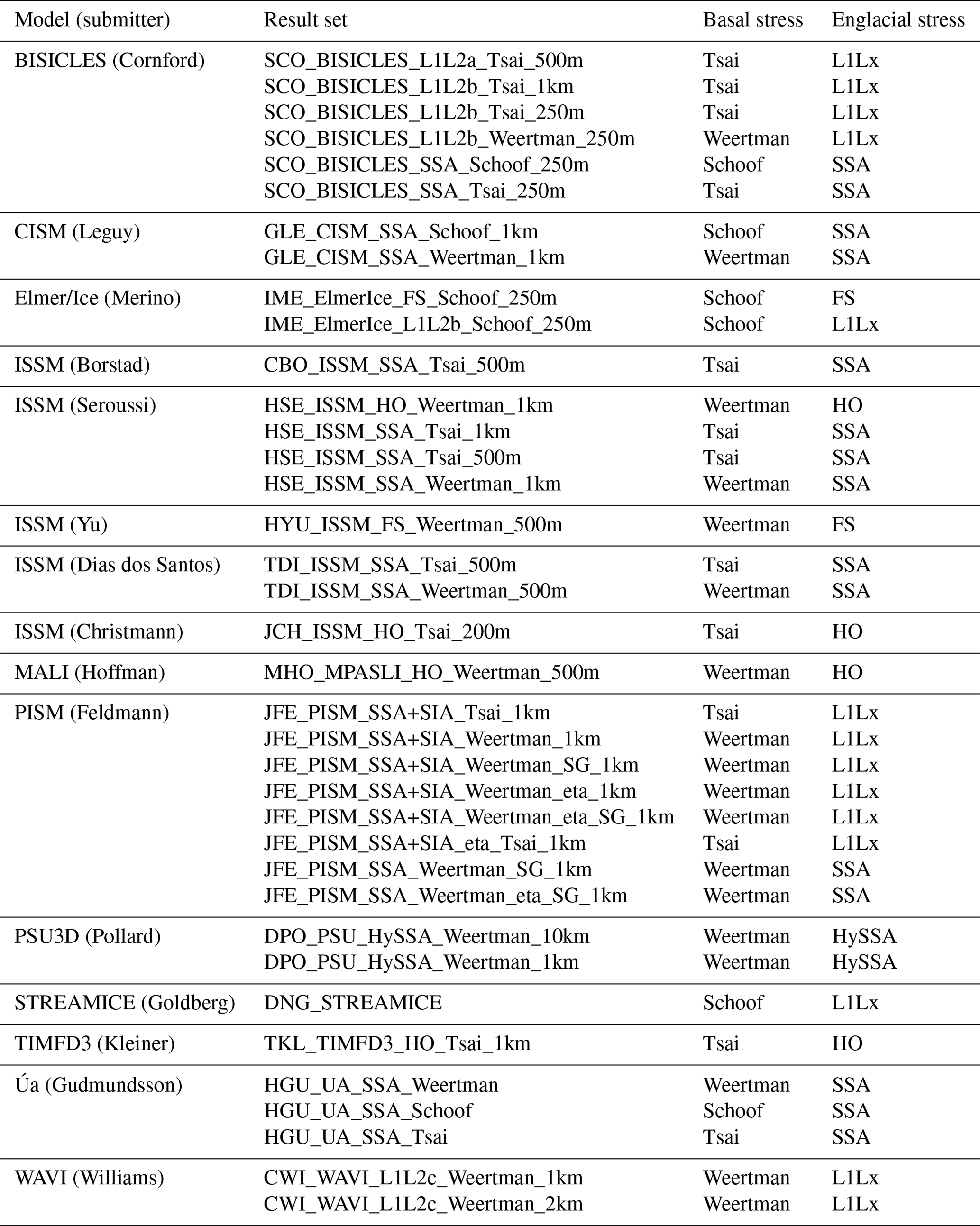
3.1 BISICLES
Six submissions are based on BISICLES (Cornford et al., 2013, 2015), a finite-volume model that employs time-evolving adaptive mesh refinement to maintain fine resolution close to the grounding line. Three vertically integrated stress approximations are included: the shallow-shelf approximation (SCO_BISICLES_SSA_Schoof_250m, SCO_BISICLES_SSA_Tsai_250m), the Schoof and Hindmarsh (2010) L1L2 approximation (SCO_BISICLES_L1L2a_Tsai_500m), and a modified L1L2 approximation that includes vertical shear in the effective viscosity but neglects it in the mass flux (the remainder). All three basal friction rules are represented. Mesh spacing at the grounding line is set to 250 m in most cases, but two coarser-resolution cases are included with Δx≥500 m and Δx≥1 km. All of the submissions apply a one-sided difference when evaluating the gravitational driving stress at the grounding line, with no other parameterization, although a subgrid friction scheme has been useful in other cases (Cornford et al., 2016).
3.2 CISM
Two submissions are based on the CISM (Lipscomb et al., 2013) model. Both employ the shallow-shelf approximation to describe englacial stresses, discretized according to the finite-element method, on a uniform mesh with 1 km horizontal resolution. Thickness transport is effected with an incremental remappping scheme (Dukowicz and Baumgardner, 2000): ice thickness and velocity data are stored at staggered locations. The difference between submissions is the choice of basal friction rule: one submission uses the Schoof (2005) scheme and the other uses the Weertman (1957) scheme. Both make use of a grounding line parameterization (Leguy et al., 2014).
3.3 Elmer/Ice
The two Elmer/Ice (Gagliardini et al., 2013, 2016) submissions differ in their treatment of englacial stresses.
IME_ElmerIce_FS_Schoof_250m is a full-Stokes model, corresponding to the majority of Elmer/Ice publications, for example Durand et al. (2009); Seddik et al. (2012). IME_ElmerIce_L1L2b_Schoof_250m is a vertically integrated model. Both are finite-element models and apply a horizontal resolution of 250 m (indicated by convergence studies to be adequate) over the region swept out by the grounding line during the Ice1 and Ice2 experiments, and a vertical discretization of 7 layers, with finer resolution toward the base. Both models employ the modified basal friction law of Eq. (4).
3.4 ISSM
Several contributions are based on the ISSM (Ice Sheet System Model), which can treat englacial stresses with a variety of approximations, from the SSA to the full-Stokes equations, using the finite-element method (Larour et al., 2011). The submissions included include one set of full-Stokes simulations (HYU_ISSM_FS_Weertman_500m), treating basal friction with the Weertman power law model, and two sets of Blatter–Pattyn approximation simulations (HSE_ISSM_HO_Weertman_1km, JCH_ISSM_HO_Tsai_200m), treating basal friction with the Weertman power law model and Coulomb-limited basal friction rules respectively. The remaining submissions are all SSA configurations, which use either the Weertman or the Coulomb-limited basal friction rules and differ in their treatment around the grounding line. HSE_ISSM_SSA_Tsai_1km, HSE_ISSM_SSA_Tsai_500m, and HSE_ISSM_SSA_Weertman_1km all make use of a fixed-in-time, nonuniform mesh of triangular elements that is refined to either 500 m or 1 km across the region swept out by the grounding line and employ the SEP1 subelement parameterization. CBO_ISSM_SSA_Tsai_500m also relies on a fixed, nonuniform mesh but chooses a different parameterization, SEP2 (Seroussi et al., 2014b), when evaluating friction in partly grounded elements. Two further submissions, TDI_ISSM_SSA_Tsai_500m and TDI_ISSM_SSA_Weertman_500m, differ from the others in their use of an evolving adaptive mesh (dos Santos et al., 2019), which is updated throughout the simulations to maintain 500 m resolutions close to the grounding line and coarser resolution elsewhere.
3.5 MALI
The MALI (MPAS-Albany Land Ice) (Hoffman et al., 2018) submission treats englacial stresses with the Blatter–Pattyn approximation and basal friction with the Weertman rule. The stress balance equation is discretized horizontally in space on an unstructured mesh of triangular finite elements, while the mass conservation equation is discretized, using the finite-volume method, on the corresponding hexagonal Voronoi tessellation. Time discretization is accomplished with the forward (explicit) Euler scheme. Basal friction around the grounding line is evaluated by computing it and the flotation criterion at the quadrature points of a fifth-order scheme, leading to a treatment comparable to SEP3 of Seroussi et al. (2014b). The experiments were carried out with 500 m spatial resolution, while the Ice1r experiment used resolutions from 4 km to 250 m.
3.6 PISM
PISM (Bueler and Brown, 2009; PISM authors, 2019; Bueler et al., 2007) employs a uniform-mesh finite-volume method to discretize the mass conservation equation and a finite-difference method to discretize the stress balance equation. It uses either the shallow-shelf approximation (SSA), or the SSA + SIA approximation, which complements SSA sliding with SIA internal deformation. All eight submissions employ a mesh spacing Δx=1 km and differ in subgrid friction interpolation versus none (Feldmann et al., 2014), SSA versus SSA + SIA, Tsai versus Weertman friction rules, and the use or otherwise of an ice thickness transformation, , to achieve better numerical results at ice sheet margins (Bueler et al., 2005, Sect. 5.2). All submissions apply a one-sided difference when evaluating the gravitational driving stress at the grounding line. Time integration is explicit, with the time step satisfying both an advection Courant–Friedrichs–Lewy (CFL) criterion determined from the SSA sliding speed and an additional constraint found by expressing the SIA as a diffusion equation (and so proportional to Δx2).
3.7 PSU3D
The two PSU3D (Pollard and DeConto, 2012) submissions represent the only HySSA model that took part in MISMIP+. This class of models is distinct from the more common types of vertically integrated models in their direct imposition of a flux across the grounding line, derived from the analytic expression of Schoof (2007), which provides consistent performance between ∼10 and ∼1 km. As a result, PSU3D has been able to simulate simulations of Antarctica lasting millions of years (Pollard and DeConto, 2009). It is a finite-difference model, based on a staggered horizontal grid, and Runge–Kutta time integration. Note that the ice-cliff failure mechanisms included in current version of this model (Pollard et al., 2015) do not arise in MISMIP+.
3.8 STREAMICE
STREAMICE (Goldberg and Heimbach, 2013) is a physical package of the MITgcm climate model (Marshall et al., 1997). It solves velocities via a finite-element method, using bilinear basis functions on quadrilateral elements on a regular grid; while its thickness is evolved via an explicit finite-volume method. Its vertically integrated stress model is based on Goldberg (2011). Near the grounding line, basal drag is regularized using a sinusoid profile where thickness is within 5 m of flotation (either above or below) – as this treatment is found to yield reversible grounding line movement in the MISMIP3d experiments. However, melt is applied to cells only where cell-averaged thickness is below flotation, i.e., no melting is applied to any cells in which basal drag is nonzero.
3.9 TIMFD3
TIMFD3 (Kleiner and Humbert, 2014) solves the stress balance equations with the LTSML (Hindmarsh, 2004) higher-order approximation together with the modified basal friction rule, Eq. (5), discretized according to the finite-difference method. In comparison to the Blatter–Pattyn approximation, the LTSML approximation considers the vertical resistive stress Rzz (van der Veen and Whillans, 1989) in the momentum balance, and thus vertical longitudinal stresses are not hydrostatic. The MISMIP+ experiments were carried out on a 1 km horizontal grid, with the vertical extent of the ice sheet treated as nine terrain-following layers, more closely spaced at the base. Coarser resolutions do not exhibit a stable grounding line. The initial state is found by taking the output from an SSA model (one of the BISICLES submissions with the same selection of A and β2) and performing a 500-year relaxation from that point. The model does not employ any kind of subgrid interpolation.
3.10 Úa
Úa (Gudmundsson, 2019; Gudmundsson et al., 2019) is an open-source finite-element ice-flow model based on a vertically integrated formulation of the momentum equations. The ice-flow equations are solved on an unstructured mesh consisting of linear, quadratic, or cubic triangular elements. Various meshing options are available, including automated mesh refinement and coarsening. When simulating the flow of marine ice sheets these meshing options allow, for example, the areas around grounding lines to be automatically highly resolved as the grounding lines migrate through the computational domain. Elements can be activated and deactivated. This enables the computational domain itself to change in the course of a run, for example when simulating the growth and decay of a large group of mountain glaciers. Ice thickness positivity is enforced using the active set method. Forward time integration can be done in a fully coupled manner, and the resulting nonlinear system is solved using the Newton–Raphson method.
3.11 WAVI
WAVI (Arthern et al., 2015) is a finite-volume model that makes use of a wavelet-based adaptive grid to accelerate the solution of the stress balance equation. Its vertically integrated stress model is derived from Goldberg (2011) and treats both membrane and simplified vertical shear stresses. Subgrid interpolation of the basal drag, gravitational driving stream, and sub-ice-shelf melt rates are deployed in the finite volumes immediately adjacent to the grounding line. Two complete submissions are included in this paper, differing only in their uniform mesh resolution. A further two partial submission are included, covering only the Ice2r experiments. These restrict nonzero sub-ice-shelf melt rates to finite volumes whose cell center is floating.
The majority of participants completed each experiment, leading to a large volume of results, many of which are in close agreement. The results of each experiment (Ice0, Ice1, and Ice2) are summarized below, concentrating on the spread of results rather than any individual model. In most cases, a substantial portion of variability in the results can be explained by straightforward groupings of the participating models: for example models that make use of the Weertman (1957) friction rule see slower grounding line migration than models employing either the Schoof (2005) or Tsai et al. (2015) rules. At the same time, distinctions that have been seen to be important in other experiments, such as the use of grounding line parameterization in MISMIP3d (Leguy et al., 2014; Seroussi et al., 2014a; Feldmann et al., 2014), appear unimportant here.
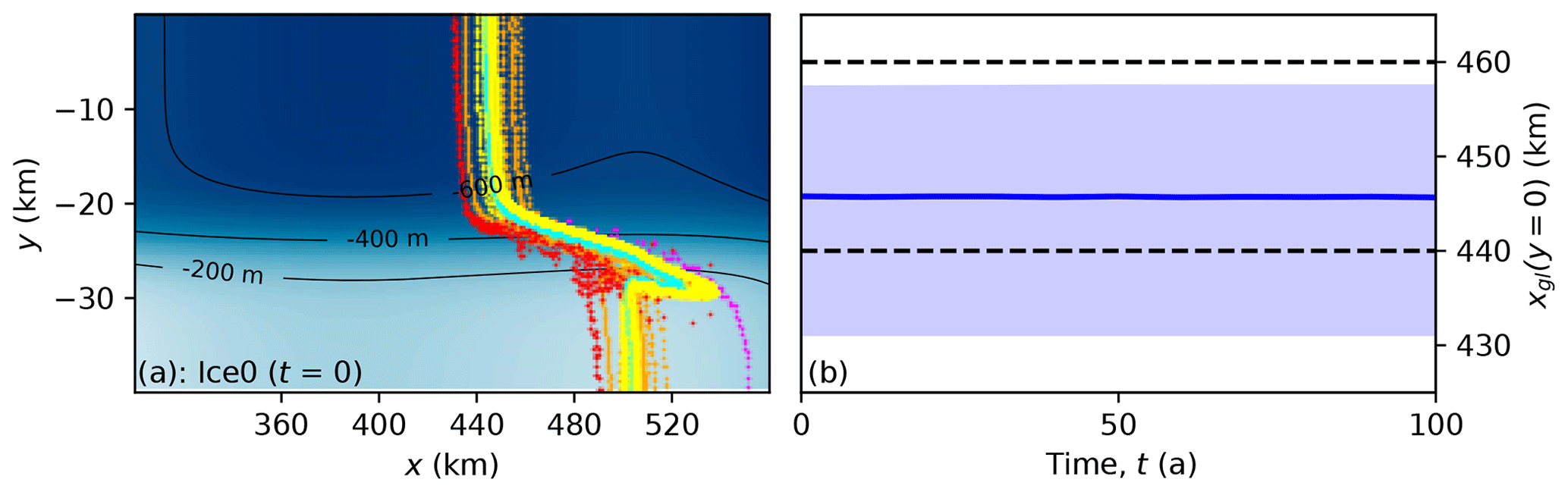
Figure 3Grounding line contours for all models with Δx≤1 km at the start of the Ice0 experiments (a) and variation over 100 years (b). In panel (a), yellow contours correspond to SSA, L1Lx, and HO models with the Coulomb-limited basal friction laws; orange contours to SSA, L1Lx, and HO models with the Weertman basal friction law; red (ISSM) and cyan (Elmer/Ice) contours to full-Stokes models; and magenta contours to HySSA models. The color map and black contours depict bedrock elevation. In panel (b), the bold line shows the grounding line position in the center of the channel, xgl(y=0), mean averaged over all models, and the shaded region depicts the maximum and minimum values. The dashed lines show the range specified in the experimental design, km
4.1 Ice0 experiments
All participating models produced a similar initial grounding line, crossing the channel in a region where the bedrock slopes upward. Figure 3 plots the grounding line for all models with Δx≤1 km at the start (t=0 a) and the grounding line position in the center of the channel, mean averaged over all models. At the start of the experiments, each grounding line intersects with the channel centerline close to xc=450 km, and the domain edge close to xe=500 km, covering most of the distance between xc and xe around the channel walls where the bedrock slopes sharply in the y direction. Most of the models also exhibit a narrow prominence at the top of this lateral bedrock slope, extending downstream from xe. There is little apparent change over time in any model, as required. Not every submission included this test, although the majority did.
Variation between the models is fairly minor. SSA, L1Lx, and HO models that employ the Coulomb-limited basal friction laws are grouped most closely, largely because there was no need to modify the default Pa−3 a−1 given in Asay-Davis et al. (2016). SSA, L1Lx, and HO models that include the Weertman basal friction law are more widely spread, with some models increasing A by as much as 25 % to achieve the specified km and others submitting results with the grounding line further upstream. Neither of the two full-Stokes models elected to modify A, but their grounding lines are close to others. Finally, the one HySSA model does produce xc≈450 km, setting Pa−3 a−1 to do so, but differs from the remaining models over the shallower bedrock with xe≈540 km.
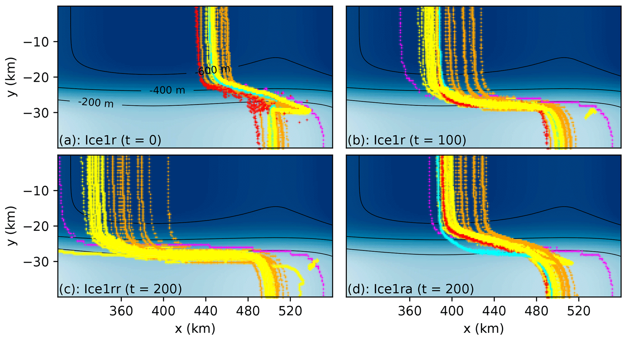
Figure 4Grounding line migration for all models with Δx≤1 km in the Ice1 experiments. The Ice1r experiment starts from the Ice0 steady-state position at t=0 a (a). Grounding lines migrate upstream while the melt rate of Eq. (7) is applied until t=100 a (b). There are two branches for t>100 a: the Ice1rr branch which continues with the same melt rate (c) and the Ice1ra branch with zero melt rate (d). Yellow contours correspond to SSA, L1Lx, and HO models with the Coulomb-limited basal friction law; orange contours to SSA, L1Lx, and HO models with the Weertman basal friction law; red (ISSM) and cyan (Elmer/Ice) contours to full-Stokes models; and magenta contours to HySSA models. The color map and black contours depict bedrock elevation.
4.2 Ice1 experiments
Figure 4 plots the grounding line for all models with Δx≤1 km over the course of the Ice1 experiments. All models see retreat of their grounding line in the center of the channel while the melt rate of Eq. (7) is imposed (the Ice1r and Ice1rr experiments) and little change outside the channel walls beyond the erosion of the prominences. The vast majority of the models also see their grounding lines readvance once the melt rate is reduced to zero (the Ice1ra experiment), albeit at a much lower rate so that the initial grounding line is not regained by the end of the experiment at t=200 a. Although all of the models are closely grouped at the start of the Ice1r experiments, a considerable spread of grounding line contours is evident after 100 years. The median retreat of midchannel grounding line position xgl(y=0) is in the region of 40 km, but the range is rather larger – close to 100 km. Within groups of models, there is a much smaller spread: around 20 km between the Coulomb-limited models, a rather larger spread between the Weertman models, and an obvious outlier in the one HySSA model with Δx≤1 km , whose midchannel grounding line position retreats by around 100 km.
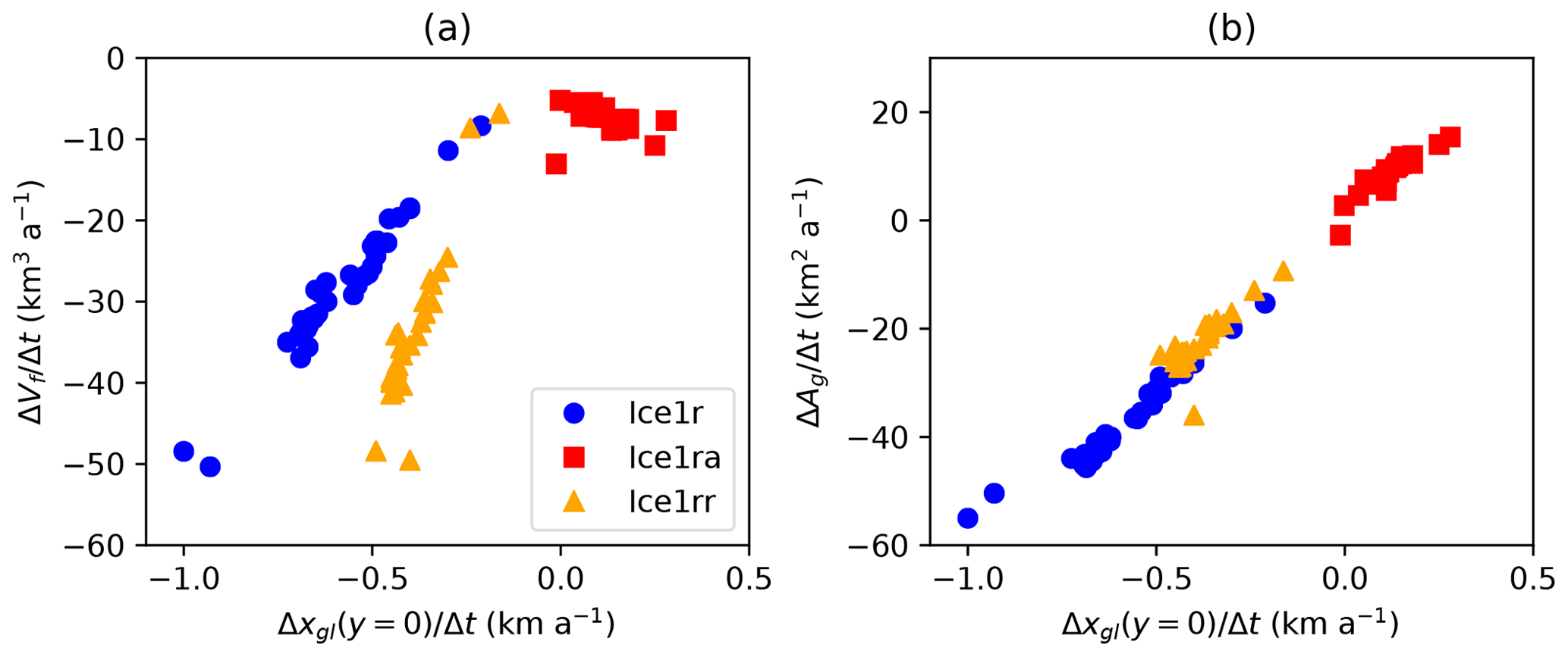
Figure 5Rates of change in midchannel grounding line position xgl(y=0) plotted against rates of change in volume above flotation Vf (a) and grounded area Ag (b). For all three of the Ice1r, Ice1ra, and Ice1rr experiments each point lies close to a straight line, as do the points , despite the considerable variation between models.
We will present the rest of the Ice1 results in terms of the midchannel grounding line position xgl(y=0), since it represents the other bulk quantities of interest well enough. The rate of change in xgl(y=0) over time represents both the rate of change in volume above flotation Vf and the rate of change in grounded area Ag (Fig. 5). A single proportional relationship links xgl(y=0) and Ag in the Ice1r, Ice1ra, and Ice1rr experiments. Ice1r and Ice1rr also see proportional relationships between xgl(y=0) and Vf, albeit with distinct constants. The exception is the Ice1ra experiment, where the readvance of the grounding line following the retreat in Ice1r is associated with a continued, mild loss of volume above flotation.

Figure 6Midchannel grounding line position plotted against time for the Ice1 experiments. Panel (a) shows the mean (solid curves) and the range (shaded regions) over all models. Panel (b) shows the mean (solid curves) and range (shaded regions) for the main subset, with individual curves (lines and symbols) for the remainder.
The majority of models behave similarly in the Ice1 experiments, so we define a number of subsets to represent the spread of results. The first of these is simply the set of all models, but since there are some clear outliers we also define a main subset comprising models which (1) completed all experiments, (2) place their Ice0 steady-state grounding line at km2, and (3) see their grounding lines retreat along the center of the channel to km. Figure 6 shows the spread in midchannel grounding line position against time for all models, the main subset, and the remainder. Of the remainder, two are the HySSA models, and the remaining two are L1Lx models. We also separate the two full-Stokes models from the lower-order approximations. The main subset then comprises HO, SSA, and L1Lx models.

Figure 7Ice1 midchannel grounding line position plotted against time for the main subset (a) and the Weertman and Coulomb-limited models (b). Weertman (W) models retreat at two-thirds the rate of Coulomb-limited (S/T) models. The larger spread in the Weertman models is attributed in large part to the spread in initial states.
One major division within the main subset is the distinction between models that employ the Weertman basal friction law (Eq. 3) and models that utilize either of the Coulomb-limited rules (Eq. 4 or Eq. 5) (Fig. 7). The mean rate of retreat seen in the Weertman models is around 0.5 km a−1 versus 0.7 km a−1 in the Coulomb-limited models, and indeed the ranges of these two subsets barely overlap. The Weertman subset also exhibits a much larger range, but we attribute this to the larger range of initial states. That larger range is due to only some participants altering the rate factor A to place the initial grounding line within the specified range, rather than any inherent difficulty with implementing the Weertman friction law.
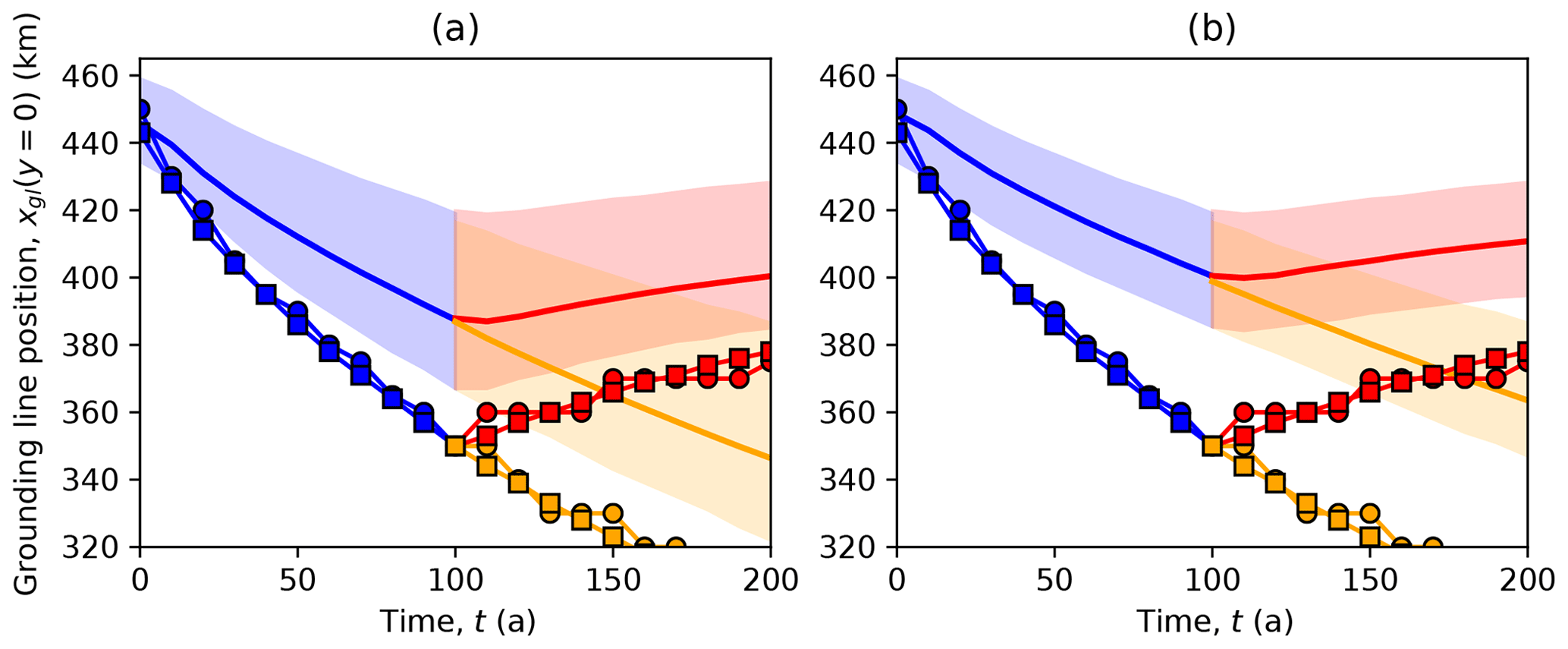
Figure 8Ice1 midchannel grounding line position plotted against time for the PSU HySSA models compared to other models. The HySSA models (solid lines with symbols) both exhibit a retreat rate around twice as fast as the main subset mean (shaded regions, panel a), and 3 times as fast as the Weertman subset mean (shaded regions, panel b).
Although the two HySSA simulations achieve an initial state close to the other models, at least in terms of grounding line positions, their transient behavior differs. Figure 8 shows both sets of HySSA results with the main subset and the Weertman subset. Their rate of retreat in Ice1r is around 1 km a−1, compared to 0.6 km a−1 for the main subset but it is more appropriate to compare to the 0.5 km a−1 of the Weertman subset given that both HySSA calculations employ that rule. Something along the same lines was seen in the MISMIP3d experiments (Pattyn et al., 2013). Note though that the HySSA simulations were computed with same model (PSU), albeit at different resolutions (1 and 10 km), so this may not be a typical result. Note also that the 1 and 10 km HySSA simulations are essentially the same, as has been the case for this class of models in other cases (Pattyn et al., 2013).
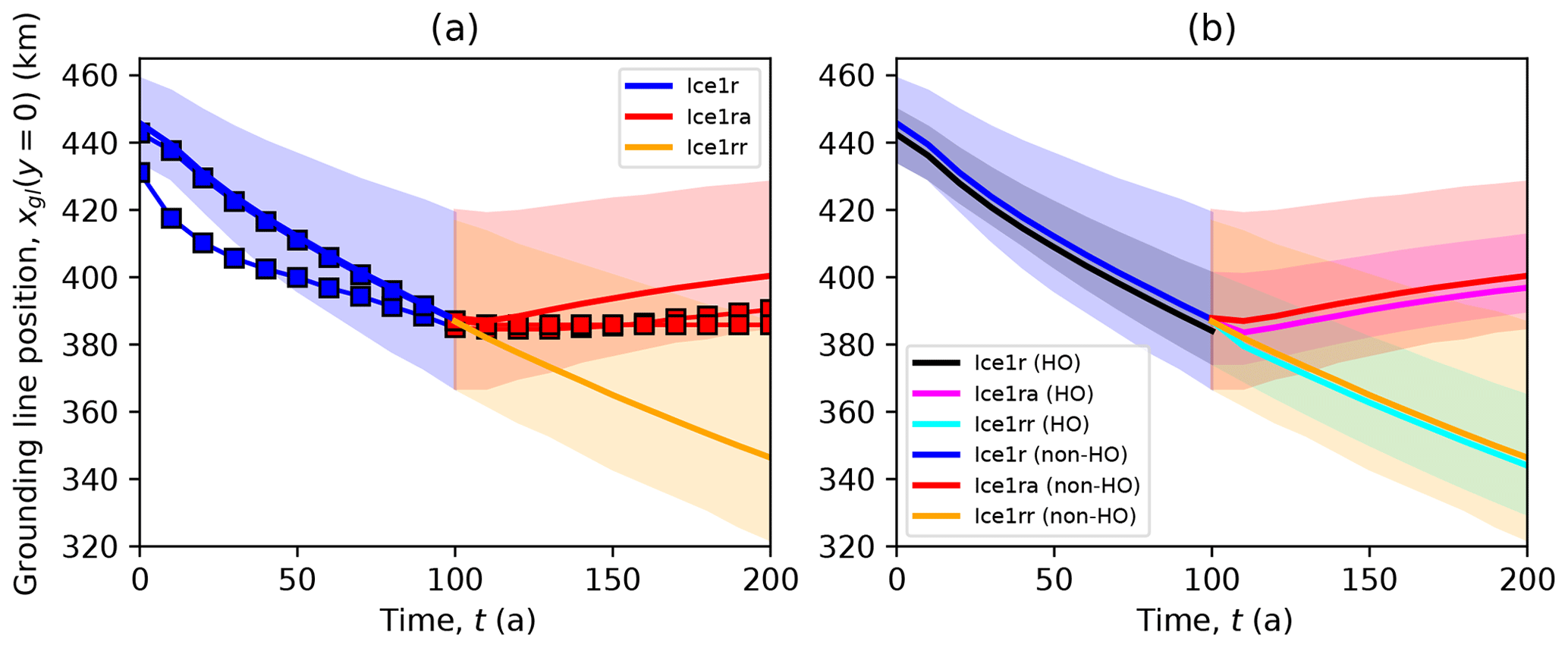
Figure 9Ice1 midchannel grounding line position plotted for Stokes, higher-order, and other models. The two full-Stokes models (symbols and lines, left panel) see a comparable rate of retreat to the main subset (shaded regions, panel a) in Ice1r but a much lower rate of advance in Ice1ra. Within the main subset, higher-order models (HO, panel b) behave in essentially the same way as the other models (non-HO, panel b).
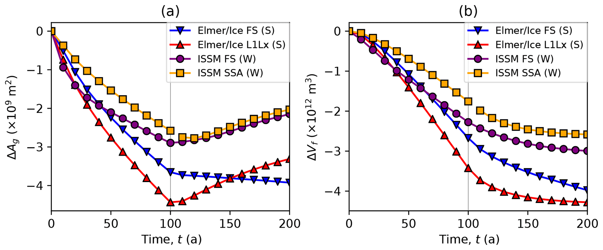
Figure 10Comparison of full-Stokes and vertically integrated models in the Ice1r (t≤100 a) and Ice1ra (t≥100 a) experiments. Panel (a) shows the change in grounded area ΔAg and panel (b) the change in volume above flotation ΔFf. “FS” indicates a full-Stokes model, “(S)” the Schoof (2005) sliding law, and “(W)” the Weertman (1957) sliding law.
The two full-Stokes models see their grounding lines retreat at the same average rate as other models while the ice shelf is ablated, but they see a lower rate of advance when the ice shelf regrows. Figure 9 compares the two full-Stokes models with the main subset, and the Ice1r retreat rate of one (IME_ElmerIce_FS_Schoof_250m) lies at the mean of the main subset. The other (HYU_ISSM_FS_Weertman_500m) retreats rather more rapidly to begin with but slows to obtain the same position after 100 years – this may be related to this model's position outside the main subset with regard to its initial state. Neither model sees rapid readvance when ice shelf ablation ceases in the Ice1ra experiment. Figure 10 compares the Stokes models with their nearest vertically integrated counterpart: the Elmer/Ice full-Stokes and L1Lx models, which both use the Schoof (2005) sliding law, and the ISSM full-Stokes and SSA models, which both use the Weertman (1957) sliding law. The ISSM full-Stokes model exhibits a similar total decrease in grounded area and both a similar regrowth and similar rate of regrowth to its SSA counterpart in Ice1ra. In contrast, the Elmer/Ice full-Stokes model sees its grounded area abate in Ice1r in a similar fashion to its L1Lx counterpart but is the only model that continues to show retreat in the Ice1ra experiment. All four models lose volume above flotation in Ice1r and Ice1ra, but the Elmer/Ice full-Stokes model sees more rapid loss in Ice1ra than the other three.
There is little variation between the higher-order and vertically integrated hydrostatic models. Figure 9 shows that the mean rate of retreat in the Ice1r experiment is close to 0.6 km a−1 over 100 years for both higher-order (HO) and vertically integrated (non-HO) models. Likewise, there is essentially no difference between HO and non-HO models in either the mean rate of further retreat in Ice1rr or the mean rate of readvance in Ice1ra. There is rather more variability between the non-HO models than between the HO-models, but that can be attributed to the smaller number of HO models (or the larger number of non-HO models).
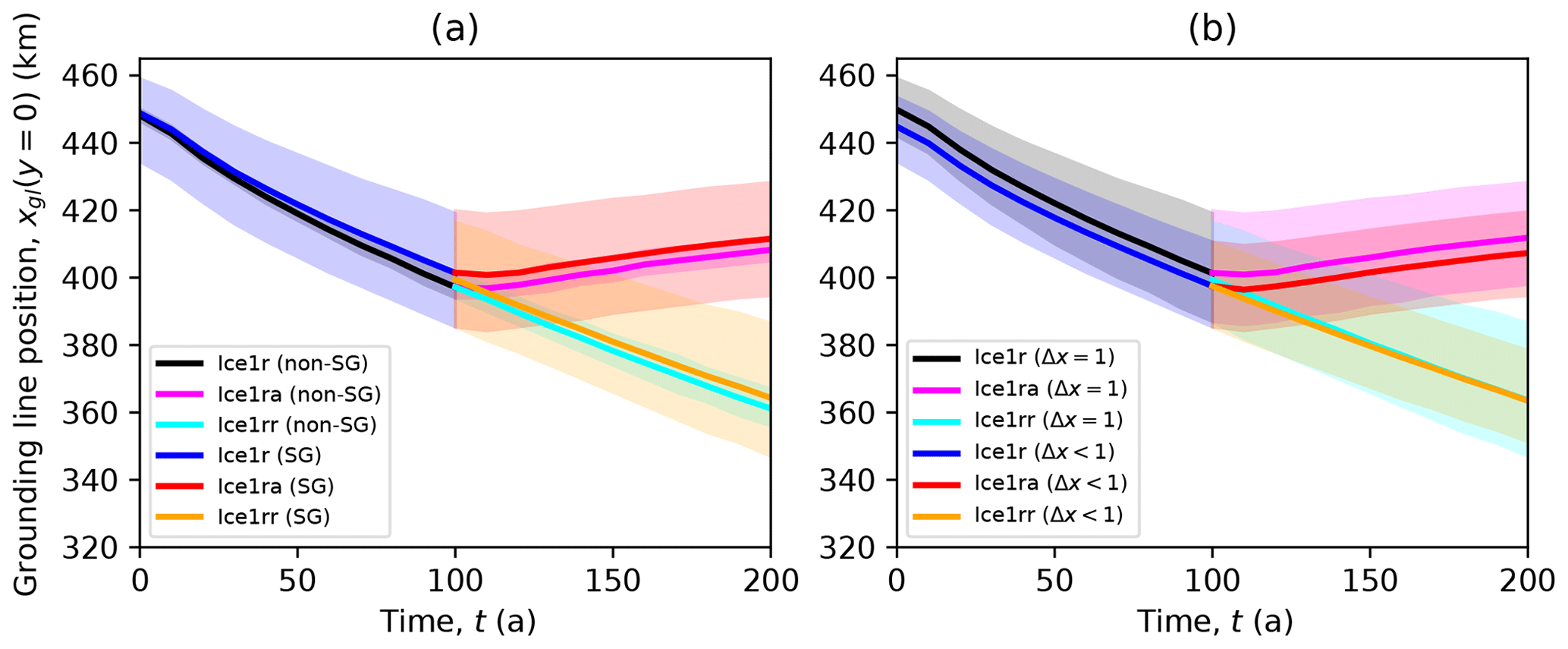
Figure 11Ice1 midchannel grounding line position plotted for models in the Weertman subgroup with varying numerical treatments. (a) Subgroups with (SG) and without (non-SG) subgrid friction schemes show similar rates of retreat and advance. (b) Likewise, the subgroup with Δx=1 km is little different from the subgroup with Δx<1 km
At least for the Δx≤1 km models included in the main subset, the choice between finer resolution or a subgrid friction scheme is unimportant. Dividing the main subset into subgroups with and without a subgrid friction scheme results in the same mean and range of grounding line migration rates, and the same is true if the subset is divided into subgroups with Δx=1 km and Δx<1 km (Fig. 11). That is not to say that neither a subgrid scheme nor a fine mesh is consequential in general. Apart from the fact that all models in the main subset have Δx≤1 km, of the 15 models that employ a subgrid scheme, only 5 have Δx<1 km, while of the 11 models that do not employ a subgrid scheme, 6 have Δx<1 km.
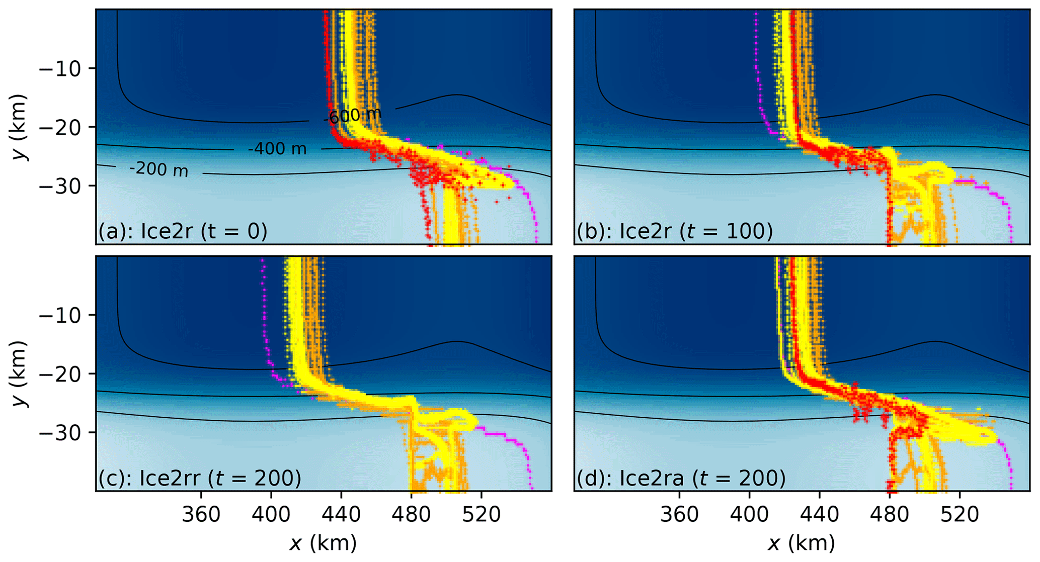
Figure 12Grounding line migration for all models with Δx≤1 km in the Ice2 experiments. The Ice2r experiment starts (as does the Ice1r experiment; see Fig. 4) from the Ice0 steady-state position at t=0 a (a). Grounding lines migrate upstream while the melt rate of Eq. (8) is applied until t=100 a (b). There are two branches for t>100 a: the Ice2rr branch which continues with the same melt rate (c) and the Ice2ra branch with zero melt rate (d). Yellow contours correspond to SSA, L1Lx, and HO models with the Coulomb-limited basal friction laws; orange contours to SSA, L1Lx, and HO models with the Weertman basal friction laws; red contours to the full-Stokes model (ISSM only); and magenta contours to HySSA models. The color map and black contours depict bedrock elevation.
Figure 13Midchannel grounding line position plotted against time for the Ice2 experiments. Panel (a) shows the mean (solid curves) and the range (shaded regions) over all models. Panel (b) shows the mean (solid curves) and range (shaded regions) for the main subset.

Figure 14Domain edge grounding line position plotted against time for the Ice2 experiments. Panel (a) shows the mean (solid curves) and the range (shaded regions) for the main subset. Panel (b) shows the mean (solid curves) and range (shaded regions) for two subgroups, Ice2A and Ice2B. Models in subgroup Ice2A see little or no grounding line retreat along the domain boundary.
4.3 Ice2 experiments
The Ice2 experiments are characterized by lower and diminishing rates of retreat compared to the Ice1 experiments. Figure 12 shows grounding line positions at the start of the Ice2r experiment, before the calving perturbations at x=480 km are applied, 100 years later, and 200 years later both with and without sustained calving at x=480 km. Figure 13 shows the grounding line positions in the center of the channel from t=0 to t=100 a. The average rate of retreat in the first 25 years of the Ice2r experiment is around 0.4 km a−1, but by the last 50 years it has dropped to 0.1 km a−1 as a thick ice shelf is formed downstream of the retreating grounding line. Compare this to the Ice1 experiment, where only a thin ice shelf is formed: the average rate of retreat is initially similar (0.6 km a−1) but does not decay substantially over time.
The major difference between models in this case is related to numerical methods. The main subset can be split into two subsets: those that exhibit no grounding line retreat along the domain wall and those that see some retreat. The first group, Ice2A, consists solely of models that do not apply a subgrid interpolation scheme when computing melt rates. The second group, Ice2B, includes models that do apply such a scheme and some that do not but have some treatment special to calving fronts (PISM variants with “eta” in their name). Figure 14 shows the variation in grounding line position at the domain wall between these two groups. Some of the Ice2B submissions have their grounding lines retreat to exactly x=480 km – the limit of nonzero melt rate in these experiments – along the wall. All of these do employ a subgrid interpolation scheme when computing melt rates and, notably, see a retreat rate that grows with their nominal mesh spacing Δx. For example, the complete WAVI submissions (with subgrid interpolation of melt rates) exhibit this retreat, whereas the supplementary results (without subgrid interpolation) do not.
Figure 15Midchannel grounding line position (a) and grounded area (b) plotted against time for the Ice2A and Ice2B models. The Ice2B models exhibit greater change in grounding line area than Ice2a, but that change is restricted to thin ice outside the channel.
The impact of this grounding line retreat along the domain wall, when it does occur, is limited in this case (but is not necessarily limited in others). Figure 15 shows both the grounding line position in the center of the channel and the grounded area as they evolve over the course of the experiment. While the loss of grounded area is significantly greater in the Ice2B models, with the mean rate of loss over the Ice2B group comparable to the maximum rate in the Ice2A group, the vast majority of the additional loss in the grounded area is restricted to the thin ice outside of the channel, and there is little difference between the two subgroups in the center of the channel.
One clear result of the MISMIP+ exercise is the degree of similarity between models. The majority of models demonstrated a similar and apparently stable equilibrium with a grounding line crossing a partly retrograde bed, an outcome which should not occur in laterally unvarying ice streams (Schoof, 2007) but does occur in buttressed systems (Goldberg et al., 2009; Gudmundsson et al., 2012). Those that did not had simply omitted the Ice0 experiment. Every model then exhibited ∼1 km a−1 grounding line retreat in response to widespread ablation of the shelf, and nearly every model exhibited a less pronounced response to ablation localized at the calving front. Likewise, nearly every model exhibited grounding line readvance once ablation ceased and ice shelves thickened. One obvious reason for such agreement is the similarity of the models, with most models featuring similar physics and mesh spacing Δx ∼1 km – which most demonstrated to be adequate. This stands in contrast to the previous MISMIP (Pattyn et al., 2012) and MISMIP3d (Pattyn et al., 2013) experiments, where models were often limited by their numerical methods.
Inasmuch as the MISMIP+ experiments are representative, the choice of basal friction law has more impact on ice stream models than the choice of englacial stress model. Higher-order models deliver essentially the same results as vertically integrated treatments, and there is also little variation between the shallow-shelf/shelfy-stream approximation (SSA) models and vertically integrated (L1Lx) models that include simplified vertical shear streams. The MISMIP+ experiments are, however, rather biased towards this conclusion, with fast sliding evident across much of the domain. This result appears to extend to the full-Stokes models, though we note that only two models of this type were included. On the other hand, models that employ the Coulomb-limited basal friction laws produce faster grounding line retreat and advance compared to models based on the Weertman rule. A similar conclusion in the context of Thwaites Glacier is reached by Yu et al. (2018)
The level of agreement between full-Stokes models and other types is less clear. Both participating full-Stokes models exhibited time-averaged grounding line retreat in line with other models in response to ice shelf ablation over 100 a, but one model (ISSM in full-Stokes mode) saw more variation over that period than other models. The other model (Elmer/Ice in full-Stokes mode) saw its grounding line continue to retreat, albeit slowly, for 100 a after ablation ceased, while ISSM saw readvance that was slower than the average across all models but within their range. In other words, where the full-Stokes models disagree with the approximate models, they also disagree with one another.
There is one more notable exception to the rule that basal friction physics matter more than englacial physics. The HySSA submissions showed the same qualitative behavior as but greater rates of grounding line retreat and advance than all of the other model types. This was also observed in the earlier MISMIP3d exercise (Pattyn et al., 2013), but the reasons are not necessarily the same. The HySSA models produced the same steady-state grounding line position as properly resolved SSA models in MISMIP3d with the same value for A, because the boundary layer approximation they rely upon was derived for that exact case, with no buttressing. In this exercise, the HySSA submissions have A around twice as large, presumably because the buttressing formulation is an informal extension to the boundary layer approximation. It may well be the case that the faster retreat is at least in part due to the slacker grounded ice (with the HySSA models setting the rate factor Pa−3 a−1 as opposed to the value Pa−3 a−1 typical of other models), but we note that the result might still carry over to realistic problems because it will be equally necessary to tune A or its equivalent when matching observations. However, recent modifications to the HySSA model bring its MISMIP+ grounding line migration rates into the envelope of the results presented here (Pollard and DeConto, 2020).
Model initial state – in this case the initial ice thickness – is also a key determinant of the response to ice shelf thinning. Models using the Weertman law had a larger spread of initial states than models based on the Coulomb-limited laws, due to model tuning, and they also showed a larger range of retreat rates when subject to strong melt rates. This is within a group of models that all began in similar states, with similar grounding line shapes crossing a retrograde slope, separated by less than 20 km: a greater difference still would be anticipated if any of the models had started from a more obviously distinct state, for example with the grounding line positioned on an entirely pro-grade slope.
Subgrid treatment of basal friction appears to be of minor importance in these experiments but does offer considerable benefit in other circumstances. Around half of the participating models employ some sort of modification to the discretization of the basal friction term in the stress balance equation, and around half do not, but there is essentially no difference between the results of these two groups. This stands in contrast to the MSIMIP3d experiment, where numerical error associated with the abrupt change in basal friction at the grounding line is a major source of differences between models at mesh resolutions comparable to and finer than the Δx∼1 km chosen by most MISMIP+ participants (Pattyn et al., 2013). Convergence studies submitted by participants to MISMIP+ (see the model data sheets in the supplement) typically indicate that the choice of Δx∼1 km is adequate for MISMIP+, subgrid friction scheme notwithstanding, while similar studies based around MISMIP3d reach the opposite conclusion: that a subgrid friction scheme permits Δx∼1 km and even coarser resolutions while the lack of such a scheme required far finer resolutions (Seroussi et al., 2014a; Feldmann et al., 2014; Gladstone et al., 2010; Leguy et al., 2014). The most obvious difference between the MISMIP3d and MISMIP+ experiments is in the shape of the grounding line and ice shelf, with MISMIP+ having a larger zone of stress transfer between floating and grounded ice, but another possible cause is the colder, stiffer ice and greater basal friction of MISMIP3d. MISMIP3d imposed Pa−3 a−1 versus Pa−3 a−1 in MISMIP+ and Pa m a1∕3 as opposed to Pa m a1∕3, so that shorter length scales in strain rates are to be expected within the grounding zone.
Subgrid treatment of melt rates – as opposed to subgrid treatment of basal friction – can result in major numerical errors, even at the moderately fine resolutions employed by the majority of participating models. The Ice2 experiments show that imposing melt on even a single cell or element that is partly grounded leads to an erroneous melt rate proportional to the mesh spacing Δx, which is not small compared to the errors caused by under-resolution of the ice dynamics. In other words, if the mesh is fine enough to obviate the error caused by subgrid melt schemes, it is also fine enough to resolve the dynamics. On the basis of these experiments, then, such treatments should be avoided. They are not to be confused with attempts to treat, for example, tidal variation in the grounding line, which may well result in strong melt rates upstream from the mean grounding line but should not produce a retreat rate that vanishes as Δx→0.
We have presented the results of the third Marine Ice Sheet Model Intercomparison Project, MISMIP+. It is distinct from its predecessors in that its initial state includes a floating ice shelf that buttresses upstream ice, so that when the ice shelf is thinned the grounded ice upstream accelerates and the grounding line retreats, and the converse when the ice shelf is allowed to regrow. More than thirty distinct submissions using 11 model programs produced similar results: an apparently stable equilibrium with a grounding line located on a retrograde slope, rapid grounding line retreat on the ablation of the ice shelf, and slower readvance on ice shelf regrowth. We found that the most important distinctions between models were the basal friction model and the initial state. In contrast, the distinction between models employing several small aspect ratio approximations to the Stokes equations was minor, at least with the limited range of model resolutions tested. The two full-Stokes models themselves do exhibit some distinct behavior, but where they agree with one another they also agree with other models. Another exception was the HySSA model, which makes use of an explicit expression for the flux across the grounding line to permit coarse (∼ 10 km) resolution and thus simulation over longer time intervals. It exhibited substantially faster grounding line migration than any other model, but recent modifications bring it within the range of other models (Pollard and DeConto, 2020).
All data used in the paper are available at https://doi.org/10.5281/zenodo.3611936 (Cornford et al., 2020).
SLC conducted the analyses and wrote the manuscript, with support from HS, XSAD, and GHG. All authors contributed model results and contributed to the manuscript.
The authors declare that they have no conflict of interest.
This article is part of the special issue “The Ice Sheet Model Intercomparison Project for CMIP6 (ISMIP6)”. It is not associated with a conference.
We thank the editor, Ayako Abe-Ouchi, and three referees, Ralf Greve, Frank Pattyn, and Fuyuki Saito, for their constructive criticism leading to an improved manuscript.
The work of Thomas Kleiner has been conducted in the framework of the PalMod project (FKZ: 01LP1511B), supported by the German Federal Ministry of Education and Research (BMBF) as the Research for Sustainability initiative (FONA). Support for Matthew Hoffman and the MALI model was provided through the Scientific Discovery through Advanced Computing (SciDAC) program and the Energy Exascale Earth System Model (E3SM) project funded by the U.S. Department of Energy (DOE), Office of Science, Biological and Environmental Research, and Advanced Scientific Computing Research programs. This research used resources of the National Energy Research Scientific Computing Center, a DOE Office of Science user facility supported by the Office of Science of the U.S. Department of Energy under contract DE-AC02-05CH11231, and resources provided by the Los Alamos National Laboratory Institutional Computing Program, which is supported by the U.S. Department of Energy National Nuclear Security Administration under contract DE-AC52-06NA25396. The material provided for the CISM model is based upon work supported by the National Center for Atmospheric Research, which is a major facility sponsored by the National Science Foundation under cooperative agreement no. 1852977.
This paper was edited by Ayako Abe-Ouchi and reviewed by Frank Pattyn, Ralf Greve, and Fuyuki Saito.
Arthern, R. J., Hindmarsh, R. C. A., and Williams, C. R.: Flow speed within the Antarctic ice sheet and its controls inferred from satellite observations, J. Geophys. Res.-Earth, 120, 1171–1188, https://doi.org/10.1002/2014JF003239, 2015. a
Asay-Davis, X. S., Cornford, S. L., Durand, G., Galton-Fenzi, B. K., Gladstone, R. M., Gudmundsson, G. H., Hattermann, T., Holland, D. M., Holland, D., Holland, P. R., Martin, D. F., Mathiot, P., Pattyn, F., and Seroussi, H.: Experimental design for three interrelated marine ice sheet and ocean model intercomparison projects: MISMIP v. 3 (MISMIP +), ISOMIP v. 2 (ISOMIP +) and MISOMIP v. 1 (MISOMIP1), Geosci. Model Dev., 9, 2471–2497, https://doi.org/10.5194/gmd-9-2471-2016, 2016. a, b, c, d, e
Bueler, E. and Brown, J.: Shallow shelf approximation as a “sliding law” in a thermomechanically coupled ice sheet model, J. Geophys. Res., 114, F03008, https://doi.org/10.1029/2008JF001179, 2009. a
Bueler, E., Lingle, C. S., Kallen-Brown, J. A., Covey, D. N., and Bowman, L. N.: Exact solutions and verification of numerical models for isothermal ice sheets, J. Glaciol., 51, 291–306, https://doi.org/10.3189/172756505781829449, 2005. a
Bueler, E., Brown, J., and Lingle, C.: Exact solutions to the thermomechanically coupled shallow ice approximation: effective tools for verfication, J. Glaciol., 53, 449–516, https://doi.org/10.3189/002214307783258396, 2007. a
Cornford, S. L., Martin, D. F., Graves, D. T., Ranken, D. F., Le Brocq, A. M., Gladstone, R. M., Payne, A. J., Ng, E. G., and Lipscomb, W. H.: Adaptive mesh, finite volume modeling of marine ice sheets, J. Comput. Phys., 232, 529–549, https://doi.org/10.1016/j.jcp.2012.08.037, 2013. a
Cornford, S. L., Martin, D. F., Payne, A. J., Ng, E. G., Le Brocq, A. M., Gladstone, R. M., Edwards, T. L., Shannon, S. R., Agosta, C., van den Broeke, M. R., Hellmer, H. H., Krinner, G., Ligtenberg, S. R. M., Timmermann, R., and Vaughan, D. G.: Century-scale simulations of the response of the West Antarctic Ice Sheet to a warming climate, The Cryosphere, 9, 1579–1600, https://doi.org/10.5194/tc-9-1579-2015, 2015. a
Cornford, S. L., Martin, D. F., Lee, V., Payne, A. J., and Ng, E. G.: Adaptive mesh refinement versus subgrid friction interpolation in simulations of Antarctic ice dynamics, Ann. Glaciol., 57, 1–9, https://doi.org/10.1017/aog.2016.13, 2016. a
Cornford, S. L., Seroussi, H., Asay-Davis, X. S., Gudmundsson, G. H., Arthern, R., Borstad, C., Christmann, J., Dias dos Santos, T., Feldmann, J., Goldberg, D., Hoffman, M. J., Humbert, A., Kleiner, T., Leguy, G., Lipscomb, W. H., Merino, N., Durand, G., Morlighem, M., Pollard, D., Ruckamp, M., Williams, C. R., and Yu, H.: Supplementary data for “Results of the third Marine Ice Sheet Model Intercomparison Project (MISMIP+)”, https://doi.org/10.5281/zenodo.3611935, 2020. a
dos Santos, T. D., Morlighem, M., Seroussi, H., Devloo, P. R. B., and Simões, J. C.: Implementation and performance of adaptive mesh refinement in the Ice Sheet System Model (ISSM v4.14), Geosci. Model Dev., 12, 215–232, https://doi.org/10.5194/gmd-12-215-2019, 2019. a
Dukowicz, J. K. and Baumgardner, J. R.: Incremental Remapping as a Transport/Advection Algorithm, J. Comput. Phys., 160, 318–335, https://doi.org/10.1006/jcph.2000.6465, 2000. a
Durand, G., Gagliardini, O., Zwinger, T., Le Meur, E., and Hindmarsh, R. C.: Full Stokes modeling of marine ice sheets: influence of the grid size, Ann. Glaciol., 50, 109–114, https://doi.org/10.3189/172756409789624283, 2009. a
Feldmann, J., Albrecht, T., Khroulev, C., Pattyn, F., and Levermann, A.: Resolution-dependent performance of grounding line motion in a shallow model compared with a full-Stokes model according to the MISMIP3d intercomparison, J. Glaciol., 60, 353–360, https://doi.org/10.3189/2014JoG13J093, 2014. a, b, c, d
Fowler, A.: Weertman, Lliboutry and the development of sliding theory, J. Glaciol., 56, 965–972, https://doi.org/10.3189/002214311796406112, 2010. a
Gagliardini, O., Zwinger, T., Gillet-Chaulet, F., Durand, G., Favier, L., de Fleurian, B., Greve, R., Malinen, M., Martín, C., Råback, P., Ruokolainen, J., Sacchettini, M., Schäfer, M., Seddik, H., and Thies, J.: Capabilities and performance of Elmer/Ice, a new-generation ice sheet model, Geosci. Model Dev., 6, 1299–1318, https://doi.org/10.5194/gmd-6-1299-2013, 2013. a
Gagliardini, O., Brondex, J., Gillet-Chaulet, F., Tavard, L., Peyaud, V., and Durand, G.: Brief communication: Impact of mesh resolution for MISMIP and MISMIP3d experiments using Elmer/Ice, The Cryosphere, 10, 307–312, https://doi.org/10.5194/tc-10-307-2016, 2016. a
Gladstone, R. M., Payne, A. J., and Cornford, S. L.: Parameterising the grounding line in flow-line ice sheet models, The Cryosphere, 4, 605–619, https://doi.org/10.5194/tc-4-605-2010, 2010. a, b
Gladstone, R. M., Warner, R. C., Galton-Fenzi, B. K., Gagliardini, O., Zwinger, T., and Greve, R.: Marine ice sheet model performance depends on basal sliding physics and sub-shelf melting, The Cryosphere, 11, 319–329, https://doi.org/10.5194/tc-11-319-2017, 2017. a
Goelzer, H., Nowicki, S., Edwards, T., Beckley, M., Abe-Ouchi, A., Aschwanden, A., Calov, R., Gagliardini, O., Gillet-Chaulet, F., Golledge, N. R., Gregory, J., Greve, R., Humbert, A., Huybrechts, P., Kennedy, J. H., Larour, E., Lipscomb, W. H., Le clec'h, S., Lee, V., Morlighem, M., Pattyn, F., Payne, A. J., Rodehacke, C., Rückamp, M., Saito, F., Schlegel, N., Seroussi, H., Shepherd, A., Sun, S., van de Wal, R., and Ziemen, F. A.: Design and results of the ice sheet model initialisation experiments initMIP-Greenland: an ISMIP6 intercomparison, The Cryosphere, 12, 1433–1460, https://doi.org/10.5194/tc-12-1433-2018, 2018. a
Goldberg, D., Holland, D. M., and Schoof, C.: Grounding line movement and ice shelf buttressing in marine ice sheets, J. Geophys. Res., 114, F04026, https://doi.org/10.1029/2008JF001227, 2009. a
Goldberg, D. N.: A variationally derived, depth-integrated approximation to a higher-order glaciological flow model, J. Glaciol., 57, 157–170, https://doi.org/10.3189/002214311795306763, 2011. a, b, c
Goldberg, D. N. and Heimbach, P.: Parameter and state estimation with a time-dependent adjoint marine ice sheet model, The Cryosphere, 7, 1659–1678, https://doi.org/10.5194/tc-7-1659-2013, 2013. a
Greve, R. and Blatter, H.: Dynamics of ice sheets and glaciers, Advances in geophysical and environmental mechanics and mathematics, Springer, Dordrecht, New York, 2009. a, b
Gudmundsson, G. H.: Ice-shelf buttressing and the stability of marine ice sheets, The Cryosphere, 7, 647–655, https://doi.org/10.5194/tc-7-647-2013, 2013. a
Gudmundsson, G. H.: Ua, Version v2019b, Zenodo, https://doi.org/10.5281/zenodo.3706624, 2019. a
Gudmundsson, G. H., Krug, J., Durand, G., Favier, L., and Gagliardini, O.: The stability of grounding lines on retrograde slopes, The Cryosphere, 6, 1497–1505, https://doi.org/10.5194/tc-6-1497-2012, 2012. a
Gudmundsson, G. H., Paolo, F. S., Adusumilli, S., and Fricker, H. A.: Instantaneous Antarctic ice-sheet mass loss driven by thinning ice shelves, Geophys. Res. Lett., 46, 13903–13909, 2019. a, b
Hindmarsh, R. C. A.: A numerical comparison of approximations to the Stokes equations used in ice sheet and glacier modeling, J. Geophys. Res., 109, F01012, https://doi.org/10.1029/2003JF000065, 2004. a, b, c, d
Hoffman, M. J., Perego, M., Price, S. F., Lipscomb, W. H., Zhang, T., Jacobsen, D., Tezaur, I., Salinger, A. G., Tuminaro, R., and Bertagna, L.: MPAS-Albany Land Ice (MALI): a variable-resolution ice sheet model for Earth system modeling using Voronoi grids, Geosci. Model Dev., 11, 3747–3780, https://doi.org/10.5194/gmd-11-3747-2018, 2018. a
Joughin, I., Smith, B. E., and Schoof, C. G.: Regularized Coulomb friction laws for ice sheet sliding: Application to Pine Island Glacier, Antarctica, Geophys. Res. Lett., 46, 4764–4771, https://doi.org/10.1029/2019GL082526, 2019. a, b, c, d
Kleiner, T. and Humbert, A.: Numerical simulations of major ice streams in Western Dronning Maud Land, Antarctica, under wet and dry basal conditions, J. Glaciol., 60, 215–232, https://doi.org/10.3189/2014JoG13J006, 2014. a
Larour, E., Seroussi, H., Morlighem, M., and Rignot, E.: Continental scale, high order, high spatial resolution, ice sheet modeling using the Ice Sheet System Model (ISSM), J. Geophys. Res.-Earth, 117, F01022, https://doi.org/10.1029/2011JF002140, 2011. a
Leguy, G. R., Asay-Davis, X. S., and Lipscomb, W. H.: Parameterization of basal friction near grounding lines in a one-dimensional ice sheet model, The Cryosphere, 8, 1239–1259, https://doi.org/10.5194/tc-8-1239-2014, 2014. a, b, c, d, e
Le Meur, E., Gagliardini, O., Zwinger, T., and Ruokolainen, J.: Glacier flow modelling: a comparison of the Shallow Ice Approximation and the full-Stokes solution, C. R. Phys., 5, 709–722, https://doi.org/10.1016/j.crhy.2004.10.001, 2004. a
Lipscomb, W. H., Price, S. F., Hoffman, M. J., Leguy, G. R., Bennett, A. R., Bradley, S. L., Evans, K. J., Fyke, J. G., Kennedy, J. H., Perego, M., Ranken, D. M., Sacks, W. J., Salinger, A. G., Vargo, L. J., and Worley, P. H.: Description and evaluation of the Community Ice Sheet Model (CISM) v2.1, Geosci. Model Dev., 12, 387–424, https://doi.org/10.5194/gmd-12-387-2019, 2019. a
MacAyeal, D. R.: Large-scale ice flow over a viscous basal sediment: Theory and application to ice stream B, Antarctica, J. Geophys. Res.-Sol. Ea., 94, 4071–4087, https://doi.org/10.1029/JB094iB04p04071, 1989. a, b
Marshall, J., Hill, C., Perelman, L., and Adcroft, A.: Hydrostatic, quasi-hydrostatic, and nonhydrostatic ocean modeling, J. Geophys. Res.-Oceans, 102, 5733–5752, https://doi.org/10.1029/96JC02776, 1997. a
Martin, D. F., Cornford, S. L., and Payne, A. J.: Millennial-Scale Vulnerability of the Antarctic Ice Sheet to Regional Ice Shelf Collapse, Geophys. Res. Lett., 46, 1467–1475, https://doi.org/10.1029/2018GL081229, 2019. a
Pattyn, F.: A new three-dimensional higher-order thermomechanical ice sheet model: Basic sensitivity, ice stream development, and ice flow across subglacial lakes, J. Geophys. Res.-Sol. Ea., 108, 2382, https://doi.org/10.1029/2002JB002329, 2003. a
Pattyn, F. and Durand, G.: Why marine ice sheet model predictions may diverge in estimating future sea level rise, Geophys. Res. Lett., 40, 4316–4320, https://doi.org/10.1002/grl.50824, 2013. a, b
Pattyn, F., Perichon, L., Aschwanden, A., Breuer, B., de Smedt, B., Gagliardini, O., Gudmundsson, G. H., Hindmarsh, R. C. A., Hubbard, A., Johnson, J. V., Kleiner, T., Konovalov, Y., Martin, C., Payne, A. J., Pollard, D., Price, S., Rückamp, M., Saito, F., Souček, O., Sugiyama, S., and Zwinger, T.: Benchmark experiments for higher-order and full-Stokes ice sheet models (ISMIP–HOM), The Cryosphere, 2, 95–108, https://doi.org/10.5194/tc-2-95-2008, 2008. a
Pattyn, F., Schoof, C., Perichon, L., Hindmarsh, R. C. A., Bueler, E., de Fleurian, B., Durand, G., Gagliardini, O., Gladstone, R., Goldberg, D., Gudmundsson, G. H., Huybrechts, P., Lee, V., Nick, F. M., Payne, A. J., Pollard, D., Rybak, O., Saito, F., and Vieli, A.: Results of the Marine Ice Sheet Model Intercomparison Project, MISMIP, The Cryosphere, 6, 573–588, https://doi.org/10.5194/tc-6-573-2012, 2012. a, b, c
Pattyn, F., Perichon, L., Durand, G., Favier, L., Gagliardini, O., Hindmarsh, R. C., Zwinger, T., Albrecht, T., Cornford, S., Docquier, D., FüRst, J. J., Goldberg, D., Gudmundsson, G. H., Humbert, A., HüTten, M., Huybrechts, P., Jouvet, G., Kleiner, T., Larour, E., Martin, D., Morlighem, M., Payne, A. J., Pollard, D., RüCkamp, M., Rybak, O., Seroussi, H., Thoma, M., and Wilkens, N.: Grounding-line migration in plan-view marine ice-sheet models: results of the ice2sea MISMIP3d intercomparison, J. Glaciol., 59, 410–422, https://doi.org/10.3189/2013JoG12J129, 2013. a, b, c, d, e, f, g, h
PISM authors: Documentation for PISM, the Parallel Ice Sheet Model: PISM, available at: https://pism-docs.org/wiki/doku.php (last access: 13 July 2020), 2019. a
Pollard, D. and DeConto, R. M.: Modelling West Antarctic ice sheet growth and collapse through the past five million years, Nature, 458, 329–332, https://doi.org/10.1038/nature07809, 2009. a
Pollard, D. and DeConto, R. M.: Description of a hybrid ice sheet-shelf model, and application to Antarctica, Geosci. Model Dev., 5, 1273–1295, https://doi.org/10.5194/gmd-5-1273-2012, 2012. a
Pollard, D. and DeConto, R.: Improvements in one-dimensional grounding-line parameterizations in an ice-sheet model with lateral variations, Geosci. Model Dev. Discuss., https://doi.org/10.5194/gmd-2020-131, in review, 2020. a, b
Pollard, D., DeConto, R. M., and Alley, R. B.: Potential Antarctic Ice Sheet retreat driven by hydrofracturing and ice cliff failure, Earth Planet. Sci. Lett., 412, 112–121, https://doi.org/10.1016/j.epsl.2014.12.035, 2015. a
Schoof, C.: The effect of cavitation on glacier sliding, Proceedings of the Royal Society A: Mathematical, Phys. Eng. Sci., 461, 609–627, https://doi.org/10.1098/rspa.2004.1350, 2005. a, b, c, d, e, f
Schoof, C.: Marine ice-sheet dynamics. Part 1. The case of rapid sliding, J. Fluid Mech., 573, 27–55, https://doi.org/10.1017/S0022112006003570, 2007. a, b, c, d
Schoof, C. and Hindmarsh, R. C. A.: Thin-Film Flows with Wall Slip: An Asymptotic Analysis of Higher Order Glacier Flow Models, Q. J. Mech. Appl. Math., 63, 73–114, https://doi.org/10.1093/qjmam/hbp025, 2010. a, b, c
Seddik, H., Greve, R., Zwinger, T., Gillet-Chaulet, F., and Gagliardini, O.: Simulations of the Greenland ice sheet 100 years into the future with the full Stokes model Elmer/Ice, J. Glaciol., 58, 427–440, https://doi.org/10.3189/2012JoG11J177, 2012. a
Seroussi, H. and Morlighem, M.: Representation of basal melting at the grounding line in ice flow models, The Cryosphere, 12, 3085–3096, https://doi.org/10.5194/tc-12-3085-2018, 2018. a
Seroussi, H., Morlighem, M., Larour, E., Rignot, E., and Khazendar, A.: Hydrostatic grounding line parameterization in ice sheet models, The Cryosphere, 8, 2075–2087, https://doi.org/10.5194/tc-8-2075-2014, 2014a. a, b, c
Seroussi, H., Morlighem, M., Larour, E., Rignot, E., and Khazendar, A.: Hydrostatic grounding line parameterization in ice sheet models, The Cryosphere, 8, 2075–2087, https://doi.org/10.5194/tc-8-2075-2014, 2014b. a, b, c
Seroussi, H., Nowicki, S., Simon, E., Abe-Ouchi, A., Albrecht, T., Brondex, J., Cornford, S., Dumas, C., Gillet-Chaulet, F., Goelzer, H., Golledge, N. R., Gregory, J. M., Greve, R., Hoffman, M. J., Humbert, A., Huybrechts, P., Kleiner, T., Larour, E., Leguy, G., Lipscomb, W. H., Lowry, D., Mengel, M., Morlighem, M., Pattyn, F., Payne, A. J., Pollard, D., Price, S. F., Quiquet, A., Reerink, T. J., Reese, R., Rodehacke, C. B., Schlegel, N.-J., Shepherd, A., Sun, S., Sutter, J., Van Breedam, J., van de Wal, R. S. W., Winkelmann, R., and Zhang, T.: initMIP-Antarctica: an ice sheet model initialization experiment of ISMIP6, The Cryosphere, 13, 1441–1471, https://doi.org/10.5194/tc-13-1441-2019, 2019. a
Tsai, V. C., Stewart, A. L., and Thompson, A. F.: Marine ice-sheet profiles and stability under Coulomb basal conditions, J. Glaciol., 61, 205–215, https://doi.org/10.3189/2015JoG14J221, 2015. a, b, c
van der Veen, C. J. and Whillans, I. M.: Force budget: I. Theory and numerical methods, J. Glaciol., 35, 53–60, https://doi.org/10.3189/002214389793701581, 1989. a
Weertman, J.: On the Sliding of Glaciers, J. Glaciol., 3, 33–38, https://doi.org/10.3189/S0022143000024709, 1957. a, b, c, d, e, f, g, h
Yu, H., Rignot, E., Seroussi, H., and Morlighem, M.: Retreat of Thwaites Glacier, West Antarctica, over the next 100 years using various ice flow models, ice shelf melt scenarios and basal friction laws, The Cryosphere, 12, 3861–3876, https://doi.org/10.5194/tc-12-3861-2018, 2018. a, b
A third rule, the Weertman–Budd rule considered in, e.g., Gladstone et al. (2017), also ensures that τb is continuous across the grounding line but is not considered here.
The requirement km was relaxed, since many participants neglected it.